Speaking Your Language: Spatial Relationships in Interpretable Emergent Communication

Abstract

Effective communication requires the ability to refer to specific parts of an observation in relation to others. While emergent communication literature shows success in developing various language properties, no research has shown the emergence of such positional references. This paper demonstrates how agents can communicate about spatial relationships within their observations. The results indicate that agents can develop a language capable of expressing the relationships between parts of their observation, achieving over 90% accuracy when trained in a referential game which requires such communication. Using a collocation measure, we demonstrate how the agents create such references. This analysis suggests that agents use a mixture of non-compositional and compositional messages to convey spatial relationships. We also show that the emergent language is interpretable by humans. The translation accuracy is tested by communicating with the receiver agent, where the receiver achieves over 78% accuracy using parts of this lexicon, confirming that the interpretation of the emergent language was successful.

1 Spatial referencing in emergent communication

Emergent communication allows agents to develop bespoke languages for their environment. While there are many successful examples of efficient (Rita et al., 2020) and compositional (Chaabouni et al., 2020) languages, they often lack fundamental aspects seen in human language, such as syntax (Lazaridou and Baroni, 2020) or recursion (Baroni, 2020). It is argued that these aspects of communication are important to improve the efficiency and generalisability of emergent languages (Baroni, 2020; Rita et al., 2024; Boldt and Mortensen, 2024). However, the current architectures, environments, and reward schemes are yet to exhibit such fundamental properties.

One such aspect is the development of deixis (Rita et al., 2024), which has been described as a way of pointing through language. Examples of temporal deixis include words such as “yesterday” or “before,” and spatial deixis include words such as “here” or “next to” (Lyons, 1977). In emergent communication, Lipinski et al. (2023) investigate how agents may refer to repeating observations, which could also be viewed from the linguistic perspective as investigating temporal deixis. However, while there are advocates to investigate how emergent languages can develop key concepts from human language (Rita et al., 2024), no work has demonstrated the emergence of relative references to specific locations within an observation, or spatial deixis.

Spatial references would be valuable in establishing shared context between agents, increasing communication efficiency by reducing the need for detailed descriptions, and adaptability, by removing the need for unique references per object. For example, instead of describing a new, previously unseen object, such as “a blue vase with intricate motifs on the table,” one could simply use spatial relationships and say “the object left of the plate.” Spatial referencing streamlines communication by leveraging the shared environment as a reference point. In dynamic environments where objects might change positions, spatial references enable agents to easily track and refer to objects without having to update their descriptions. This enhances communication efficiency and improves interaction and collaboration between agents. These elements may also help the evolved language become human interpretable, allowing the development of trustworthy emergent communication (Lazaridou and Baroni, 2020; Mu and Goodman, 2021).

This paper therefore explores how agents can develop communication with spatial references. While Rita et al. (2024) posit that the emergence of these references might require complex settings, we show that even agents trained in a modified version of the simple referential game (Lazaridou et al., 2018; Lewis, 1969) can develop spatial references. This resulting language is analysed using a collocation measure, Normalised Pointwise Mutual Information (NPMI) adapted from computational linguistics. Our choice of NPMI is motivated by its ability to measure the strength of associations between message parts and their context, making it a valuable tool for gaining insights into the underlying structure of the emergent language. We show how the agents compose such spatial references, providing the first evidence of a syntactic structure, and showing that the emergent language can be interpreted by humans.

2 Development of a spatial referential game

Current emergent communication environments have not produced languages incorporating spatial references. To address this, we develop a referential game (Lazaridou et al., 2018) environment where an effective language requires communication about spatial relationships. In the referential game, there are two agents, a sender and a receiver. The sender observes a vector and transmits its compressed representation through a discrete channel to the receiver. The receiver observes a set of vectors together with the sender’s message. One of these vectors is the same as the one the sender has observed. The receiver’s goal is to correctly identify the vector the sender has described, among other vectors referred to as distractors. The simplicity of the referential games enables the reduction of extraneous factors which could impact the emergence of spatial references, such as transfer learning of the vision network or exploring action spaces in more complex environments.

In this work, the sender’s input is an observation in the form of a vector $\bm{o}=[o_{1},o_{2},o_{3},o_{4},o_{5}]$, where $\forall o\in\{-1,0,1\ldots 59\}$. The vector $\bm{o}$ is always composed of $5$ integers. The observation includes a $-1$ in only one position, $\bm{o}_{3}=-1$ for $\bm{o}=[x,x,-1,x,x]$, to indicate the target integer for the receiver to identify. $\bm{o}$ represents a window into a longer sequence $\bm{s}$, which is randomly generated using the integers $\{0\ldots 59\}$ without repetitions. This sequence is visible to the receiver, but not to the sender. As the target’s position in the sequence is unknown to the sender, it has to rely on the relative positional information present in its observation, necessitating the use of spatial referencing.

Due to the window into the sequence being of length $5$, it is necessary to shift the window when it approaches either extent of the sequence. The window is then shifted to the other side, maintaining the size of $5$. For example, given a short sequence $\bm{s}=[7,5,2,12,10,4,3,15,16,13,14,6,9,8,11,1]$, if the selected target is $1$, since there are no integers to the right of $1$ the vector $\bm{o}$ would be $\bm{o}=[6,9,8,11,-1]$ where it is shifted to the left as it approaches this rightmost extent of the sequence.

Due to the necessity of maintaining the window size, some observations provide additional positional information to the sender agent. Given the same example sequence $\bm{s}$, we can categorise all observations into $5$ types. The begin and begin+1, where the target integer is either at, or one after, the beginning of the sequence, $\bm{o}=[-1,5,2,12,10]$ or $\bm{o}=[7,-1,2,12,10]$. The end and end-1, where the target integer is either at, or one before, the end of the sequence, $\bm{o}=[6,9,8,11,-1]$ or $\bm{o}=[6,9,8,-1,1]$. The most common case is the middle observation, where the target integer is anywhere in the sequence, excluding the first, second, second to last, and last positions, $\bm{o}=[12,10,-1,3,15]$. Given a window of length $5$, only $4$ specific target integer positions per sequence can result in the other observations (begin, begin+1, end-1, and end). All other target integer positions within the sequence fall into the middle category, as they do not occupy the first, second, second to last, or last positions. Consequently, the majority of the target integer positions result in a middle type observation.

The sender’s output is a message defined as a vector $\bm{m}=[m_{1},m_{2},m_{3}]$, where $m\in\{1\ldots 26\}$. $26$ is chosen to allow for a high degree of expressivity, with the agents being able to use over 17k different messages, while also matching the size of the Latin alphabet, reflecting one of the common alphabet lengths. The vector $\bm{m}$ is always composed of $3$ integers.

The receiver’s input is an observation consisting of three vectors: the sender’s message $\bm{m}$, the sequence $\bm{s}$, and the set of distractor integers together with the target integers $\bm{td}$. The distractor integers are randomly generated, without repetitions, given the same range of integers as the original sequence $\bm{s}$, $\{0\ldots 59\}$, excluding the target object itself.

For example, given the sequence $\bm{s}=[7,5,2,12,10,4,3,15,16,13,14,6,9,8,11,1]$, and the sender’s observation $\bm{o}=[4,3,-1,16,13]$, the vector $\bm{td}$ could be $\bm{td}=[7,15,11,9]$, with $15$ being the target that the receiver needs to identify. The sender could produce a message $\bm{m}=[3,1,1]$, which would mean that the target integer is one after the integer $3$. This message would then be passed to the receiver, together with $\bm{s}$ and $\bm{td}$. The receiver would then have to correctly understand the message $\bm{m}$ (that the target is one after $3$) and find the integer $3$ together with the following integer in the sequence $\bm{s}$. Having identified the target $15$ given the message $\bm{m}$ and the sequence $\bm{s}$, it would output the correct position of this target in the $\bm{td}$ vector, $2$, since $\bm{td}_{2}=15$.

3 Agent Architecture

The agent architecture follows that of the most commonly used EGG agents (Kharitonov et al., 2019). This architecture is used to maintain consistency with the common approaches in emergent communication research (Kharitonov et al., 2019; Chaabouni et al., 2019, 2020; Ueda and Washio, 2021; Lipinski et al., 2023), increasing the generalization of the results presented in this work.

The sender agent, shown in Figure 1(a), receives a single input, the vector $\bm{o}$, which is passed through the first GRU of the sender. The resulting hidden state is used as the initial hidden state for the message generation GRU (Cho et al., 2014). The message generation GRU is used to produce the message, character by character, using the Gumbel-Softmax reparametrization trick (Jang et al., 2017; Mordatch and Abbeel, 2018; Kharitonov et al., 2019). The sequence of character probabilities generated from the sender is used to output the message $\bm{m}$.

$\bm{m}$ is input to the receiver agent, shown in Figure 1(b), together with the full sequence $\bm{s}$ and the targets and distractors $\bm{td}$. The message is processed by the first receiver GRU, which produces a hidden state used as the initial hidden state for the GRU processing the sequence $\bm{s}$. This is the only change from the standard EGG architecture (Kharitonov et al., 2019). This additional GRU allows the receiver agent to process the additional input sequence $\bm{s}$, using the information contained within the message $\bm{m}$. The goal of this GRU is to use the information provided by the sender to correctly identify which integer from the sequence $\bm{s}$ is the target integer. The final hidden state from the additional GRU is multiplied with an embedding of the targets and distractors, to output the receiver’s prediction. This prediction is in the form of the index of the target within $\bm{td}$.

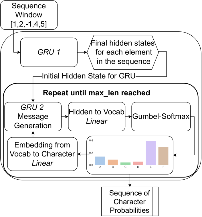
(a) The sender architecture.

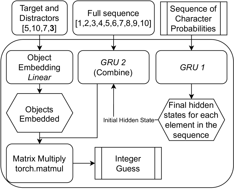
(b) The receiver architecture.

Figure 1: The sender and receiver architectures. Adapted from (Lipinski et al., 2023).

Following the commonly used approach (Kharitonov et al., 2019), agent optimisation is performed using the Gumbel-Softmax reparametrization (Jang et al., 2017; Mordatch and Abbeel, 2018), allowing for direct gradient flow through the discrete channel. The agents’ loss is computed by applying the cross entropy loss, using the receiver target prediction and the true target label. The resulting gradients are passed to the Adam optimiser and backpropagated through the network. Detailed training hyperparameters are provided in Appendix A.

4 Message interpretability and analysis using NPMI

To analyse spatial references in emergent language, a way to identify their presence is essential. In discrete emergent languages, interpretation is typically done by either using dataset labels in natural language (Dessì et al., 2021), or by qualitative analysis of specific messages (Havrylov and Titov, 2017). However, both of these techniques require message-meaning pairs, and so neither would be able to identify the presence of spatial references, as the labels for spatial relationships that the agents refer to would not necessarily be available. One approach that could overcome this problem is emergent language segmentation using Harris’ Articulation Scheme, recently employed by Ueda et al. (2023). Ueda et al. (2023) compute the conditional entropy of each character in the emergent language, segmenting the messages where the conditional entropy increases. However, even after language segmentation, there is no easy way to interpret the segments, as no method has been proposed to map them to specific meanings.

We present an approach to both segment the emergent language and map the segments to their meanings. We use a collocation measure called Normalised Pointwise Mutual Information (NPMI) (Bouma, 2009), often used in computational linguistics (Yamaki et al., 2023; Lim and Lauw, 2024; Thielmann et al., 2024). It is used to determine which messages are used for which observations and to analyse how the messages are composed, including whether they are trivially compositional (Korbak et al., 2020; Steinert-Threlkeld, 2020; Perkins, 2021). By applying a collocation measure to different parts of each message as well as the whole message, we can address the problems of both segmentation and interpretation of the message segments. This approach allows any part of the message to carry a different meaning. For example, if an emergent message contains segments that frequently appear in contexts involving specific integers, NPMI can help identify these segments and their meanings based on their statistical association with those integers.

NPMI is a normalised version of the Pointwise Mutual Information (PMI) (Church and Hanks, 1989), which is a measure of association between two events. PMI is widely used in computational linguistics, to measure the association between words (Paperno and Baroni, 2016; Han et al., 2013). Normalising the PMI measure results in its codomain being defined between $-1$ and $1$, with $-1$ indicating a purely negative association (events never occurring together), $0$ indicating no association (events being independent), and $1$ indicating a purely positive association (events always occurring together). Normalised PMI is used for convenience when defining a threshold at which we consider a message or n-gram to carry a specific meaning, as the threshold can be between $0$ and $1$, instead of unbounded numbers in the case of PMI.

To determine which parts of each message are used for a given meaning, two algorithms are proposed.

1. PMI_nc The algorithm to measure non-compositional monolithic messages, most often used for target positional information (begin+1 (Section 2)); and

2. PMI_c the algorithm to measure trivially compositional messages and their n-grams, used to refer to different integers in different positions.

A visual representation of the different types of messages that the algorithms can identify is provided in Figure 2. The PMI_nc algorithm can identify any non-compositional messages, while the PMI_c algorithm identifies both position variant and invariant compositional messages. The positional variance of the emergent language means that the position of an n-gram in the message also carries a part of its meaning. In this work, n-grams refer to a contiguous sequence of n integers from the sender’s message. Consequently, in one message there are $3$ unigrams ($m_{1}$, $m_{2}$, $m_{3}$), two bigrams ([$m_{1}$, $m_{2}$], [$m_{2}$, $m_{3}$]), and one trigram (the whole message [$m_{1}$, $m_{2}$, $m_{3}$]).

Figure 2 shows that in the position invariant case, the bigram $[5,6]$ always carries the meaning of $4$. While in the position variant case, the bigram $[5,6]$ in position $1$ of the message means $4$, but $[5,6]$ in position $2$ of the message means $8$. This can also be interpreted as the position of the bigram containing additional information, meaning a single “word” could be represented as a tuple of the bigram and its position in the message, as both contribute to its underlying information. Non-compositional messages are monolithic, the whole message carries the entire meaning. For example, message $[5,6,8]$ means the target is in the first position, while $[5,6,6]$ means the target is one to the right of $9$, even though the two messages share the bigram $[5,6]$.

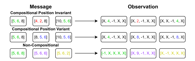
Figure 2: Examples of the different types of message compositionality that are possible to identify using the PMI algorithms.

The PMI_nc algorithm

The PMI_nc algorithm calculates the NPMI per message by first building a dictionary of all counts of each message being sent, together with an observation that may provide positional information (begin+1) or refer to an integer in a given position ($1$ left of the target). The counts of that message and the counts of the observation, including the integer position, are also collected. For example, consider the observation $\bm{o}=[4,-1,15,16,13]$. For the corresponding message $\bm{m}$, the counts for each integer in each position relative to the target would increase by $1$ ($left1[4]+=1$, $right1[15]+=1$ ). The count for the message signifying begin+1 would also be increased. Given these counts, the algorithm then estimates the probabilities of all respective events (messages, positional observations, and integers in given positions) and calculates the NPMI measure.

The PMI_c algorithm

The PMI_c algorithm first creates a dictionary of all possible n-grams, given the message space ($m$) and maximum message length ($3$). The list of all possible n-grams is pruned to contain only the n-grams present in the agents’ language, avoiding unnecessary computation in the later parts of the algorithm. Given the pruned list of n-grams, the algorithm checks the context in which the n-grams have been used. The occurrence of each n-gram is counted, together with the n-gram position in the messages and the context in which it has been sent, or the integers in the observation. The n-gram position in the message is considered to account for the possible position variance of the compositional messages.

Consider the previous example, with $\bm{o}=[4,-1,15,16,13]$ and a message $\bm{m}=[11,13,5]$. For all n-grams ($[11],[13],[5],[11,13],$ ) of the message, all integers are counted, irrespective of their positions ($counts[4]+=1$, $counts[15]+=1$, ).

Given these counts, the PMI_c algorithm estimates the NPMI measure for all n-grams and all integers in the observations. These probabilities are estimated from the dataset using the count of their respective occurrences divided by the number of all observations/messages.

Once the NPMI measure is obtained for the n-gram-integer pairs, the algorithm calculates the NPMI measure for n-grams and referent positions or the positions of the integer in the observation the message refers to. For example, given an observation $\bm{o}=[4,-1,15,16,13]$, if the message contains an n-gram which has been identified as referring to the integer $15$, the rest of the message (the unigram or bigram, depending on the length of the integer n-gram) is counted as a possible reference to that position, in this case, to position $right1$, or $1$ to the right of the target. This procedure follows for all messages, building a count for each time an n-gram was used together with a possible n-gram for an integer. These counts are used to calculate the NPMI measure for n-gram and position pairs.

The PMI_c algorithm also accounts for the possible position invariance of the n-grams, where in the message the n-gram appears. This is achieved by calculating the respective probabilities regardless of the position of the n-gram in the message, by summing the individual counts for each n-gram position.

Pseudocode

We provide a condensed pseudocode for both algorithms in Algorithm 1. In the case of the PMI_nc, the n-grams in the pseudocode would be whole messages, trigrams. This base pseudocode would then be duplicated, interpreting the context as either an observation that may provide positional information (begin+1) or an integer.

For the PMI_c algorithm, only the unigrams and bigrams would be evaluated. The base pseudocode would also be duplicated, once for the integer in a given position, and second for the referent position. Each would be used as the context in which to evaluate the NPMI for each n-gram. A detailed commented pseudocode for both the PMI_nc and PMI_c algorithms is available in Algorithm 2 and Algorithm 3 in Appendix B, respectively.

1 Gather ngram_counts, context_counts, joint_counts, n_grams;

2 for each n-gram $g$ in position $p$ and context $c$ do

3       $P(g,p)=\texttt{ngram\_counts}[g]\cdot\frac{\displaystyle 1}{\displaystyle\texttt{total n-grams}}$;

4       $P(c)=\texttt{context\_counts}[c]\cdot\frac{\displaystyle 1}{\displaystyle\texttt{total contexts}}$;

5       $P(g,p;c)=\texttt{joint\_counts}[(g,c)]\cdot\frac{\displaystyle 1}{\displaystyle\texttt{total n-grams}}$;

6       $\text{NPMI}(g,p;c)=\log_{2}\frac{\displaystyle P(g,p,c)}{\displaystyle P(g)P(c)}\cdot\frac{\displaystyle 1}{\displaystyle-\log_{2}P(g,p,c)}$;

7      

8 end for

return NPMI;

Algorithm 1 PMI Algorithm Base

Both algorithms use two hyperparameters: a confidence threshold $t_{c}$ and top_n $t_{n}$. The confidence threshold refers to the value of the NPMI measure at which a message or n-gram can be considered to refer to the given part of the observation unambiguously. To account for polysemy (where one symbol can have multiple meanings), the agents can use a single n-gram to refer to multiple integers. This is given by the second hyperparameter, top_n, which sets the degree of the polysemy, or the number of integers to be considered for a given n-gram.

5 Spatial referencing experiments

The agent pairs are trained over $16$ different seeds to verify the results’ significance. All agent pairs achieve above $98\%$ accuracy on the referential task, showing that the agents develop a way to communicate about spatial relationships in their observations. The analysis provided in this section is based on the messages collected from the test dataset after the training has finished.

The two hyperparameters, $t_{c}$ and $t_{n}$ (Section 4), governing the NPMI measure have been determined through a grid search to maximise the understanding of the emergent language, by maximising the translation accuracy. The results in this section are obtained using the best-performing values for each of the hyperparameters.

5.1 Emergence of non-compositional spatial references

Using the PMI_nc algorithm, we detect the emergence of messages tailored to convey the positional information contained in the observations. As mentioned in Section 2, sender observations which require shifting convey additional information about the position of the target within the sequence. In over $90\%$ of agent pairs, these observations are assigned unique messages, used only for each kind of observation, begin, begin+1, end-1 and, end.

In $20\%$ of runs which develop these specialised messages, the same repeating character is used to convey the message. The characters used for these observations are reserved only for these kinds of observations. For example, in one of the runs the agents use character $11$ to signify the beginning of the sequence, with the character $11$ being used only in two contexts: as the messages $[11,11,11]$ to signify begin, or as a message $[0,11,11]$ to signify begin+1. In other cases, characters are fully reserved for specific messages. $22$ is used only for end, in the message $[22,22,22]$.

The emergence of non-compositional references used for other observations is also detected using the $PMI_{nc}$ algorithm. Such messages refer to a specific integer in a specific position of the sender observation, $o_{5}=10$. While we allow for polysemy of the message in our analysis using $t\_n=[1,2,3,5,10,15]$, we observe the highest translation accuracy with $t\_n=1$, indicating that the non-compositional messages do not have any additional meanings.

5.2 Emergence of compositional spatial references

Using the $PMI_{c}$ algorithm, we also detect the emergence of compositional spatial references for 25% of agent pairs. Such messages are composed of two parts, a positional reference and an integer reference. The positional reference specifies where a given integer can be found in the observation, in relation to the masked target integer $-1$. The integer reference specifies which integer the positional reference is referring to. For example, one pair of agents has assigned the unigram $7$ to mean that the target integer is $2$ to the right of the given integer, and the bigram $[0,2]$ to mean the integer $18$. Together, a message can be composed $[7,0,2]$, which means that the target integer for the receiver to identify is $2$ to the right of the integer $18$, $\bm{o}=[18,X,-1,X,X]$. This allows the sender to identify the target integer exactly, given the sequence $\bm{s}$.

5.3 Evaluating interpretation validity and accuracy

To ensure the validity of our message analysis, we present two null hypotheses, which, if falsified, would indicate the mappings generated by the NPMI measure to be correct.

Hypothesis 1 (H1)

If the correlations exist, but are more complex (require non-trivial compositionality (Perkins, 2021), or are highly context dependent (Nikolaus, 2023)) then the accuracy should be near chance, or $20\%$, when using the identified mappings.

Hypothesis 2 (H2)

If the positional components of compositional messages are incorrectly identified, or do not carry any meaning, then their inclusion should not increase the accuracy.

Given the messages identified by the NPMI method, we test H1 and H2 by using a dictionary of all messages successfully identified, given a value of both NPMI hyperparameters $t_{n}$ and $t_{c}$. A dataset is generated to contain only targets which can be described with the messages present in the dictionary.

For the non-compositional messages, the dataset is generated by selecting a message from the dictionary at random, and creating an observation that can be described with that message. Given a non-compositional message that corresponds to the target being on the right of the integer $15$, an observation $\bm{o}=[1,15,-1,5,36]$ would be created. Analogously, for non-compositional positional messages such as begin an observation $\bm{o}=[-1,15,8,5,36]$ would be created.

For the compositional messages, we create the observations by randomly selecting a positional component and an integer component from the dictionary. For example, given the unigram $7$ meaning that X is 2 to the left of the target, we could select the bigram $[8,14]$ corresponding to the integer $30$. The observation created could then be $\bm{o}=[30,8,-1,36,5]$. The dataset creation process for the compositional messages also checks if the observations can be described given the two n-grams in their required positions within the message.

To test H2, a dataset is created using only the integers that can be described by the dictionaries, randomly selecting integer components from the dictionary, and creating the respective observations. This process also accounts for the required positions of the message components so that a message describing the observation can always be created. For example, if the unigram $9$ described the integer $11$, and the bigram $[5,1]$ described the integer $6$, a corresponding observation could be $\bm{o}=[11,6,-1,8,9]$. The positions of the integers in the observations are chosen at random. By generating both compositional datasets using a stochastic process, we do not assume a specific syntax. Rather, the syntax can only be identified by looking at messages which were understood by the receiver.

These datasets, together with their respective dictionaries, are then used to query the receiver agent, testing if the messages are identified correctly. We run this test for all of our trained agents, with the dictionaries that were identified for each agent pair. We provide the details of this evaluation in Table 1.

Table 1: Accuracy improvements using the NPMI-based dictionary, $\pm$ denotes the 1-sigma standard deviation. Non-Compositional Positional refers to messages such as begin or end, Non-Compositional Integer refers to the non-compositional monolithic messages describing both the position and the integer, Compositional-NP refers to messages only containing the identified integer components, and the Compositional-P which refers to messages containing both the identified integer and positional components.

Dict Type	$t_{n}$	$t_{c}$	Average Accuracy	Maximum Accuracy
Non-Compositional Positional	$1$	$0.9$	0.90 $\pm$0.03	0.94
Non-Compositional Integer	$1$	$0.5$	0.36 $\pm$0.004	0.37
Compositional-NP	$1$	$0.5$	0.22 $\pm 0.02$	0.28
Compositional-P	$1$	$0.5$	0.30 $\pm 0.21$	0.78

Using just the non-compositional positional messages, we observe a significant increase in the performance of the agents, compared to random chance accuracy of 20%. This proves H1 false, showing that at least some messages do not require complex functions to be composed, or contextual information to be interpreted. As the accuracy for these messages reaches over 90% on average, we argue that the NPMI method has captured almost all the information transmitted using these messages.

As mentioned in H2, we examine the impact of the positional components and whether they carry the information the NPMI method has identified. We, therefore, separate the compositional analysis into two parts: Compositional-NP, where there are no positional components, and Compositional-P, which includes positional components. In the Compositional-NP case, the agents achieve a close to random accuracy, whereas, in the Compositional-P case, agents achieve above random accuracy, with some agent pairs reaching over 75% accuracy. This falsifies our H2 null hypothesis, showing that the NPMI method has successfully identified the positional information contained in the messages, together with the integer information.

6 Discussion

Having falsified both H1 and H2, we confirmed the validity of the language analysis. To provide human interpretability of the emergent language, we use the NPMI method to create a dictionary providing an understanding of both the positional and compositional messages. We present an excerpt from an example dictionary in Table 2. With human interpretability, we can gain a deeper understanding of the principles underlying the agents’ communication protocol.

We posit that the emergence of compositional spatial references points to a first emergence of a simple syntactic structure in an emergent language. Both of the n-grams in our example from Section 5.2, also shown in Table 2, are assigned specific positions in the message by the agents. The unigram $7$ must always be in the first position of the message, while the bigram $[0,2]$ must always be in the second position. We can interpret these messages as using the Subject-Verb-Object (SVO) word order, with the subject target being implied, the verb being the unigram $7$ representing “is two to the right of”, and the object being $[0,2]$ representing the object of “integer 18”. The emergence of this structure shows that even though referential games have been considered obsolete in recent research (Chaabouni et al., 2022; Rita et al., 2024), a careful design of the environment may yet elicit more of the fundamental properties of natural language.

We hypothesise that the emergence of non-compositional spatial references tailored to specific observations, such as begin+1, is due to observation sparsity. Compositionality would bring no benefit since the observations which they describe are usually rare, representing 1-2% of the dataset and are monolithic, begin, begin+1, end-1, and end. We therefore argue that the emergence of non-compositional references in these cases is advantageous, since these messages could be further compressed. With a linguistic parsimony pressure (Rita et al., 2020; Chaabouni et al., 2019) applied, these messages could be more efficient at transmitting the information contained within these observations than compositional ones.

Table 2: Example dictionary of the agents’ messages and their meanings

Message	Type	Meaning
$[11,11,11]$	Non-Compositional Positional	begin
$[0,11,11]$	Non-Compositional Positional	begin+1
$[10,10,10]$	Non-Compositional Positional	end-1
$[18,18,18]$	Non-Compositional Positional	end
$[12,16,14]$	Non-Compositional Integer	15 is 1 left of target
$[15,X,X]$	Compositional Positional	X is 2 left of target
$[7,X,X]$	Compositional Positional	X is 2 right of target
$[X,0,17]$	Compositional Integer	Integer 1
$[X,0,2]$	Compositional Integer	Integer 18
$[X,8,14]$	Compositional Integer	Integer 30

7 Limitations

The accuracy for the Non-Compositional Integer, and Compositional-P messages averages about 33%. While still above random, showing that some meaning is captured in non-compositional messages, it points to there being more to be understood about these messages. We hypothesise this may be due to the higher degree of message pragmatism, or context dependence (Nikolaus, 2023). Our method of message generation, using randomly selected parts, may not be able to capture the complexity of the messages. For example, the context in which they are used might be crucial for some n-grams, requiring the use of a specific n-gram instead of another when referring to certain integers, or when specific integers are present in the observation. Just like in English, certain verbs are only used with certain nouns, such as “pilot a plane” vs “pilot a car”. While the word “pilot” in the broad sense refers to operating a vehicle, it is not used with cars specifically. This may also be the case for the emergent language. For compositional messages, an additional issue may be that some messages are non-trivially compositional, using functions apart from simple concatenation to convey compositional meaning (Perkins, 2021), making them impossible to analyse with the NPMI measure. However, these issues may be addressed by scaling the emergent communication experiments as the languages become more general with the increased complexity of their environment (Chaabouni et al., 2022).

8 Conclusion

Recent work in the field of emergent communication has advocated for better alignment of emergent languages with natural language (Rita et al., 2024; Boldt and Mortensen, 2024), such as through the investigation of deixis (Rita et al., 2024). Aligned to this approach, we provide a first reported emergent language containing spatial references (Lyons, 1977), together with a method to interpret the agents’ messages in natural language. We show that agents can learn to communicate about spatial relationships with over 90% accuracy. We identify both compositional and non-compositional spatial referencing, showing that the agents use a mixture of both. We hypothesise why the agents choose non-compositional representations of observation types which are sparse in the dataset, arguing that this behaviour can be used to increase communicative efficiency. We show that, using the NPMI language analysis method, we can create a human interpretable dictionary, of the agents’ own language. We confirm that our method of language interpretation is accurate, achieving over 94% accuracy for certain dictionaries.

Appendix A Training Details

The computational resources needed to reproduce this work are shown in Table 3, with the hyperparameters in Table 4. The Table 3 shows resources required for all training and evaluation. The processors used were a mixture of Intel Xeon Silver 4216s and AMD EPYC 7502s. The GPUs used for the training were a mixture of NVIDIA Quadro RTX 8000s, NVIDIA Tesla V100s, and NVIDIA A100s. These nodes used in our experiments were hosted on an internal cluster. The development process consumed more compute, which we estimate would have added 10 CPU and GPU hours, to account for experimentation.

Table 3: Compute resources

Resource	Value (1 Run)	Value (Training Total)	Value (Evaluation & Analysis)
Nodes	1	8	1
CPU	16 cores	128 cores	64 cores
GPU	1	8	1
Memory	50 GB	400 GB	120 GB
Storage	1 GB	32 GB	32 GB
Wall time	2 hours	240 hours	24 hours

Table 4: Hyperparameters

Parameter	Value
Epochs	1000
Optimizer	Adam
Learning Rate $\alpha$	0.001
Gumbel-Softmax Temperature	[1.0]
Training Dataset Size	200k
Test Dataset Size	20k
No. Distractors	4
No. Points	60
Message Length	3
Vocabulary Size	26
Sender Hidden Size	64
Receiver Hidden Size	64

Appendix B Algorithm Descriptions

For our pseudocode we will be using the Python assignments convention, $=$ and $\leftarrow$ are equivalent, and $x$+=$1$ is equivalent to $x\leftarrow x+1$. The algorithms presented are for $top\_n=1$. To improve the computational efficiency. the probability of the integer appearing is statically defined as $\frac{1}{60}$ for $top\_n=1$, or in Equation 1 for $top\_n>1$. In the case of $top\_n>1$ we use the probability for the integer as per Equation 1, to account for the polysemy, the probability for any of $top\_n$ integers occurring in the observation. The lower part of the binomial is $4$, as there are $4$ integers that can be sampled from the $60$ possible integers, instead of $5$, as we exclude the target integer.

$$p(integers)=\frac{\binom{60}{4}-\binom{60-top\_n}{4}}{\binom{60}{4}}$$ (1)

Additionally, in the PMI_c algorithm, we specify a probability to equal to $0.98$ in Line 5 and Line 5. This is a simplification of the calculation for clarity of the pseudocode. This probability is instead obtained using the count of a given type of observation, divided by the number of total observations. This calculation is performed for each type of observation, begin, begin+1, end, end-1 and middle. The probability of the middle observation is very close to $1$, being on average $0.98$, while the other probabilities are on average $0.005$. Since the any observation is most common, we included its value in the pseudocode.

Data: $O\_M$ ;

  # All observations together with sent messages

1

Data: $L=len(O\_M)$ ;

  # Total number of observations with sent messages

2

Data: $S=[begin,begin+1,end-1,end]$ ;

  # List of positional observations

3

Result: $pmi_{nc}[m][NPMI]$

4

5$pmi_{nc}=$ dict;

6for $o,m\in O\_M$ do

       $pmi_{nc}[m][count]$ += 1 ;

        # Message occurrences

7       for $pos\in S$ do

8             if $o==pos$ then

                   $pmi_{nc}[pos][count]$ += 1 ;

                    # Positional observations count

                   $pmi_{nc}[m][pos]$ += 1 ;

                    # Message sent with positional observation

9                  

10             end if

11            

12       end for

13      for $integer\in o$ do

             $pmi_{nc}[m][integer\_pos][integer]$ += 1 ;

              # Message sent with integer in given position

14            

15       end for

16      

17 end for

18

19for $pos\in S$ do

       $posit_{total}=pmi_{nc}[pos][count]$ ;

        # Count of positional observations

       $p(pos)=\frac{posit_{total}}{L}$;

        # Estimate observation probability

20       for $m\in pmi_{nc}[m]$ do

             $m_{total}=pmi_{nc}[m][count]$ ;

              # Total count of message

21            

            $ms_{total}=pmi_{nc}[m][pos]$ ;

              # Total count of message with positional obs

22            

            $p(m)=\frac{m_{total}}{L}$ ;

              # Estimate message probability

23            

            $p(m,pos)=\frac{ms_{total}}{L}$ ;

              # Estimate joint probability

24            

25            $h(m,pos)=-\log_{2}(p(m,pos))$ ;

26            $pmi(m,pos)=\log_{2}(\frac{p(m,pos)}{p(m)p(pos)})$;

27            $npmi(m,pos)=\frac{pmi(m,pos)}{h(m,pos)}$;

28            $pmi_{nc}[m][NPMI]=npmi(m,pos)$;

29       end for

30      

31 end for

32for $pos\in pmi_{nc}[m]$ do

33       for $integer\in pmi_{nc}[m][pos]$ do

             $p(pos)=\frac{1}{60}$;

              # Estimated observation probability for 60 integers

34            

            $m_{total}=pmi_{nc}[m][count]$ ;

              # Total count of message

35            

            $ms_{total}=pmi_{nc}[m][pos][integer]$ ;

              # Total count of message with integer in given position

36            

            $p(m)=\frac{m_{total}}{L}$ ;

              # Estimate message probability

37            

            $p(m,pos)=\frac{ms_{total}}{L}$ ;

              # Estimate joint probability

38            

39            $h(m,pos)=-\log_{2}(p(m,pos))$ ;

40            $pmi(m,pos)=\log_{2}(\frac{p(m,pos)}{p(m)p(pos)})$;

41            $npmi(m,pos)=\frac{pmi(m,pos)}{h(m,pos)}$;

42            $pmi_{nc}[m][pos][integer][NPMI]=npmi(m,pos)$;

43       end for

44      

45 end for

Algorithm 2 The PMI_nc algorithm

Input: $t_{c}$ ;

  # Confidence value

1

Data: $O\_M$ ;

  # All observations together with sent messages

2

Data: $L=len(O\_M)$ ;

  # Total number of observations with sent messages

3

Data: $ngrams$ ;

  # List of all message ngrams present in $O\_M$

4

Result: $pmi_{c}[m][NPMI]$

5

6$pmi_{c}=$ dict;

;

 # First we identify ngrams corresponding to integers.

7 for $ngram\in ngrams$ do

8       for $o,m\in O\_M$ do

9             if $ngram\in m$ then

                   $pmi_{c}[ngram][count]$ += 1 ;

                    # Total ngram occurrences

                   $pmi_{c}[ngram][ngram\_pos][count]$ += 1 ;

                    # ngram occurrences including ngram position

10                   for $integer\in o$ do

                         $pmi_{c}[ngram][integer][count]$ += 1 ;

                          # ngram sent with integer in given position

                         $pmi_{c}[ngram][ngram\_pos][integer][count]$ += 1 ;

                          # ngram in given position sent with integer in given position

11                        

12                   end for

13                  

14             end if

15            

16       end for

17      

18 end for

19

;

 # Calculate integer NPMI.

20 for $ngram\in ngrams$ do

       ;

       # Position variant NPMI.

21       for $pos\in pmi_{c}[ngram][ngram\_pos]$ do

22            

            $p(integer)=\frac{1}{60}$;

              # Estimated observation probability for 60 integers

23            

            $integer_{p}=max(pmi_{c}[ngram][integer][count])$;;

              # Find integer with highest co-ocurrence given position

24            

25            $ngram_{pos}=pmi_{c}[ngram][ngram\_pos][count]$ ;

26            $p(ngram_{pos})=\frac{ngram_{pos}}{L}$

27            $p(ngram_{pos},integer)=\frac{pmi_{c}[ngram][ngram\_pos][integer][count]}{L}$;

28            $h(ngram_{pos},integer)=-\log_{2}(p(ngram_{pos},integer))$;

29            $pmi(ngram_{pos},integer)=\log_{2}(\frac{p(ngram_{pos},integer)}{p(ngram_{pos})p(integer)})$;

30            $npmi(ngram_{pos},integer)=\frac{pmi(ngram_{pos},integer)}{h(ngram_{pos},integer)}$;

31            $pmi_{c}[ngram][ngram\_pos][integer]=npmi(ngram_{pos},integer)$;

32       end for

      ;

       # Position invariant NPMI.

33      

      $integer=max(pmi_{c}[ngram][integer][count])$;;

        # Find integer with highest co-ocurrence

34      

      $p(integer)=\frac{1}{60}$;

        # Estimated observation probability for 60 integers

35      

36      $ngram_{total}=pmi_{c}[ngram][count]$ ;

      $p(ngram)=\frac{ngram_{total}}{L\times(4-len(ngram))}$ ;

        # If ngram is length 1, it could appear 3 times per message

37      

38      $p(ngram,integer)=\frac{pmi_{c}[ngram][integer][count]}{L}$;

39      $h(ngram,integer)=-\log_{2}(p(ngram,integer))$;

40      $pmi(ngram,integer)=\log_{2}(\frac{p(ngram,integer)}{p(ngram)p(integer)})$;

41      $npmi(ngram,integer)=\frac{pmi(ngram,integer)}{h(ngram,integer)}$;

42      $pmi_{c}[ngram][integer]=npmi(ngram,integer)$;

43 end for

Algorithm 3 The PMI_c algorithm

36

;

 # Now we identify ngrams corresponding to referent positions.

37 $ngram_{pr}$ = dict;

;

 # Prune ngrams with NPMI below $c$

38 for $ngram\in pmi_{c}$ do

39       for $integer\in pmi_{c}[ngram]$ do

40             if $pmi_{c}[ngram][integer]<t_{c}$ then

41                   del $pmi_{c}[ngram][integer]$;

42             end if

43            for $pos\in pmi_{c}[ngram]$ do

44                   for $integer\in pmi_{c}[ngram][pos]$ do

45                         if $pmi_{c}[ngram][pos][integer]<t_{c}$ then

46                               del $pmi_{c}[ngram][pos][integer]$;

47                         end if

48                        

49                   end for

50                  

51             end for

52            

53       end for

54      

55 end for

56

;

 # Find messages with integer ngrams

57 for $ngram\in pmi_{c}[ngram]$ do

58       for $o,m\in O\_M$ do

             ;

             # Position variant ngram

59             if $pmi_{c}[ngram][pos]$ then

60                   if $ngram\in m[pos]$ then

                         $new\_ngram=m-ngram$;

                          # Get leftover ngram

                         $pr=pos(pmi_{c}[ngram][pos][integer],msg)$ ;

                          # Get the possible referent position

                         $ngram_{pr}[new\_ngram][pr][count]+=1$ ;

                          # Count leftover ngram occurence

                         $ngram_{pr}[new\_ngram][pos][pr][count]+=1$ ;

                          # Count leftover ngram occurence in given positions

61                        

62                   end if

63                  

64             end if

            ;

             # Position invariant ngram

65             else

66                   if $ngram\in m$ then

                         $new\_ngram=m-ngram$ ;

                          # Get leftover ngram

                         $pr=pos(pmi_{c}[ngram][integer],msg)$ ;

                          # Get the possible referent position

                         $ngram_{pr}[new\_ngram][pr][count]+=1$ ;

                          # Count leftover ngram occurence

                         $ngram_{pr}[new\_ngram][pos][pr][count]+=1$ ;

                          # Count leftover ngram occurence in given positions

67                        

68                   end if

69                  

70             end if

71            

72       end for

73      

74 end for

Algorithm 4 The PMI_c algorithm cont.

71

;

 # Calculate referent position NPMI.

72 for $ngram\in ngram_{pr}$ do

73       for $pr\in ngram_{pr}[ngram][pr]$ do

             ;

             # Position variant NPMI.

74             for $pos\in ngram_{pr}[ngram][pos][pr]$ do

75                  

                  $p(pr)=0.98$;

                    # Estimated observation probability for given position

76                   $ngram_{pos}=ngram_{pr}[ngram][pos][pr][count]$ ; $p(ngram_{pos})=\frac{ngram_{pos}}{L}$ $p(ngram_{pos},pr)=\frac{ngram_{pr}[ngram][pos][pr][count]}{L}$; $h(ngram_{pos},pr)=-\log_{2}(p(ngram_{pos},integer))$; $pmi(ngram_{pos},pr)=\log_{2}(\frac{p(ngram_{pos},pr)}{p(ngram_{pos})p(pr)})$; $npmi(ngram_{pos},pr)=\frac{pmi(ngram_{pos},pr)}{h(ngram_{pos},pr)}$; $pmi_{c}[ngram][pos][pr]=npmi(ngram_{pos},pr)$;

77             end for

            ;

             # Position invariant NPMI.

             $p(pr)=0.98$;

              # Estimated observation probability for given position

78            

            $ngram=max(ngram_{pr}[ngram][pr][count])$ ;

              # Find highest positional reference count

79            

80            $p(ngram)=\frac{ngram}{L}$;

81            $p(ngram,pr)=\frac{ngram_{pr}[ngram][pr][count]}{L}$;

82            $h(ngram,pr)=-\log_{2}(p(ngram,integer))$;

83            $pmi(ngram,pr)=\log_{2}(\frac{p(ngram,pr)}{p(ngram)p(pr)})$;

84            $npmi(ngram,pr)=\frac{pmi(ngram,pr)}{h(ngram,pr)}$;

85            $pmi_{c}[ngram][pr]=npmi(ngram,pr)$;

86       end for

87      

88 end for

89

Algorithm 5 The PMI_c algorithm cont.

References

- Baroni (2020) Marco Baroni. Rat big, cat eaten! Ideas for a useful deep-agent protolanguage. ArXiv preprint, abs/2003.11922, 2020.
- Boldt and Mortensen (2024) Brendon Boldt and David R. Mortensen. A Review of the Applications of Deep Learning-Based Emergent Communication. Transactions on Machine Learning Research, 2024.
- Bouma (2009) Gerlof J. Bouma. Proc. of gscl. In Von der Form zur Bedeutung: Texte automatisch verarbeiten - From Form to Meaning: Processing Texts Automatically, volume 30, pages 31–40, 2009.
- Chaabouni et al. (2019) Rahma Chaabouni, Eugene Kharitonov, Emmanuel Dupoux, and Marco Baroni. Anti-efficient encoding in emergent communication. In Proc. of NeurIPS, pages 6290–6300, 2019.
- Chaabouni et al. (2020) Rahma Chaabouni, Eugene Kharitonov, Diane Bouchacourt, Emmanuel Dupoux, and Marco Baroni. Compositionality and generalization in emergent languages. In Proc. of ACL, pages 4427–4442, 2020.
- Chaabouni et al. (2022) Rahma Chaabouni, Florian Strub, Florent Altché, Eugene Tarassov, Corentin Tallec, Elnaz Davoodi, Kory Wallace Mathewson, Olivier Tieleman, Angeliki Lazaridou, and Bilal Piot. Emergent communication at scale. In Proc. of ICLR, 2022.
- Cho et al. (2014) Kyunghyun Cho, Bart van Merriënboer, Caglar Gulcehre, Dzmitry Bahdanau, Fethi Bougares, Holger Schwenk, and Yoshua Bengio. Learning phrase representations using RNN encoder–decoder for statistical machine translation. In Proc. of EMNLP, pages 1724–1734, 2014.
- Church and Hanks (1989) Kenneth Ward Church and Patrick Hanks. Word association norms, mutual information, and lexicography. In Proc. of ACL, pages 76–83, 1989.
- Dessì et al. (2021) Roberto Dessì, Eugene Kharitonov, and Marco Baroni. Interpretable agent communication from scratch (with a generic visual processor emerging on the side). In Proc. of NeurIPS, pages 26937–26949, 2021.
- Han et al. (2013) Lushan Han, Tim Finin, Paul McNamee, Anupam Joshi, and Yelena Yesha. Improving word similarity by augmenting PMI with estimates of word polysemy. IEEE TKDE, 25(6):1307–1322, 2013.
- Havrylov and Titov (2017) Serhii Havrylov and Ivan Titov. Emergence of language with multi-agent games: Learning to communicate with sequences of symbols. In Proc. of NeurIPS, pages 2149–2159, 2017.
- Jang et al. (2017) Eric Jang, Shixiang Gu, and Ben Poole. Categorical reparameterization with gumbel-softmax. In Proc. of ICLR, 2017.
- Kharitonov et al. (2019) Eugene Kharitonov, Rahma Chaabouni, Diane Bouchacourt, and Marco Baroni. EGG: a toolkit for research on emergence of lanGuage in games. In Proc. of EMNLP, pages 55–60, 2019.
- Korbak et al. (2020) Tomasz Korbak, Julian Zubek, and Joanna Raczaszek-Leonardi. Measuring non-trivial compositionality in emergent communication. In 4th Workshop on Emergent Communication, NeurIPS 2020, 2020.
- Lazaridou and Baroni (2020) Angeliki Lazaridou and Marco Baroni. Emergent Multi-Agent Communication in the Deep Learning Era. ArXiv preprint, abs/2006.02419, 2020.
- Lazaridou et al. (2018) Angeliki Lazaridou, Karl Moritz Hermann, Karl Tuyls, and Stephen Clark. Emergence of linguistic communication from referential games with symbolic and pixel input. In Proc. of ICLR, 2018.
- Lewis (1969) David Kellogg Lewis. Convention: A Philosophical Study. Wiley-Blackwell, 1969.
- Lim and Lauw (2024) Jia Peng Lim and Hady W. Lauw. Aligning Human and Computational Coherence Evaluations. Computational Linguistics, pages 1–58, 2024.
- Lipinski et al. (2023) Olaf Lipinski, Adam J. Sobey, Federico Cerutti, and Timothy J. Norman. It’s About Time: Temporal References in Emergent Communication. ArXiv preprint, abs/2310.06555, 2023.
- Lyons (1977) John Lyons. Deixis, space and time. In Semantics, volume 2, pages 636–724. Cambridge University Press, 1977.
- Mordatch and Abbeel (2018) Igor Mordatch and Pieter Abbeel. Emergence of grounded compositional language in multi-agent populations. In Sheila A. McIlraith and Kilian Q. Weinberger, editors, Proc. of AAAI, pages 1495–1502, 2018.
- Mu and Goodman (2021) Jesse Mu and Noah D. Goodman. Emergent communication of generalizations. In Proc. of NeurIPS, pages 17994–18007, 2021.
- Nikolaus (2023) Mitja Nikolaus. Emergent Communication with Conversational Repair. In Proc. of ICLR, 2023.
- Paperno and Baroni (2016) Denis Paperno and Marco Baroni. Squibs: When the whole is less than the sum of its parts: How composition affects PMI values in distributional semantic vectors. Computational Linguistics, 42(2):345–350, 2016.
- Perkins (2021) Hugh Perkins. Neural networks can understand compositional functions that humans do not, in the context of emergent communication. ArXiv preprint, abs/2103.04180, 2021.
- Rita et al. (2020) Mathieu Rita, Rahma Chaabouni, and Emmanuel Dupoux. “LazImpa”: Lazy and impatient neural agents learn to communicate efficiently. In Proc. of CoNLL, pages 335–343, 2020.
- Rita et al. (2024) Mathieu Rita, Paul Michel, Rahma Chaabouni, Olivier Pietquin, Emmanuel Dupoux, and Florian Strub. Language Evolution with Deep Learning, 2024.
- Steinert-Threlkeld (2020) Shane Steinert-Threlkeld. Toward the Emergence of Nontrivial Compositionality. Philosophy of Science, 87(5):897–909, 2020.
- Thielmann et al. (2024) Anton Thielmann, Arik Reuter, Quentin Seifert, Elisabeth Bergherr, and Benjamin Säfken. Topics in the Haystack: Enhancing Topic Quality through Corpus Expansion. Computational Linguistics, pages 1–37, 2024.
- Ueda and Washio (2021) Ryo Ueda and Koki Washio. On the relationship between Zipf’s law of abbreviation and interfering noise in emergent languages. In Proc. of ACL, pages 60–70, 2021.
- Ueda et al. (2023) Ryo Ueda, Taiga Ishii, and Yusuke Miyao. On the Word Boundaries of Emergent Languages Based on Harris’s Articulation Scheme. In Proc. of ICLR, 2023.
- Yamaki et al. (2023) Ryosuke Yamaki, Tadahiro Taniguchi, and Daichi Mochihashi. Holographic CCG Parsing. In Proc. of ACL, pages 262–276, 2023.