3D Voxel Maps to 2D Occupancy Maps for Efficient Path Planning for Aerial and Ground Robots

Abstract

This article introduces a novel method for converting 3D voxel maps, commonly utilized by robots for localization and navigation, into 2D occupancy maps that can be used for more computationally efficient large-scale navigation, both in the sense of computation time and memory usage. The main aim is to effectively integrate the distinct mapping advantages of 2D and 3D maps to enable efficient path planning for both unmanned aerial vehicles (UAVs) and unmanned ground vehicles (UGVs). The proposed method uses the free space representation in the UFOMap mapping solution to generate 2D occupancy maps with height and slope information. In the process of 3D to 2D map conversion, the proposed method conducts safety checks and eliminates free spaces in the map with dimensions (in the height axis) lower than the robot’s safety margins. This allows an aerial or ground robot to navigate safely, relying primarily on the 2D map generated by the method. Additionally, the method extracts height and slope data from the 3D voxel map. The slope data identifies areas too steep for a ground robot to traverse, marking them as occupied, thus enabling a more accurate representation of the terrain for ground robots. The height data is utilized to convert paths generated using the 2D map into paths in 3D space for both UAVs and UGVs. The effectiveness of the proposed method is evaluated in two different environments.

I INTRODUCTION

A map is a fundamental component of robotics, serving key roles in localization, trajectory planning, and obstacle avoidance. The most common form of map representation is the metric grid-based map, in either 2D or 3D formats. Both 3D and 2D grid-based maps have their respective advantages: 3D maps are more accurate representations of the world and offer greater detail and precision, while 2D maps offer the advantage in terms of performance and minimality, particularly with respect to computational efficiency and memory usage. Therefore, utilizing both representations can be beneficial [1] for path planning in autonomous robots. A common approach involves creating and managing two separate 2D and 3D mapping solutions, by either converting 3D scans used in 3D mapping to 2D scans for creating the 2D map [2, 3, 4] or using multiple sensors [5]. However, this leads to the challenge of managing two different mapping frameworks on a single robot, potentially resulting in mismatched maps. This paper aims to effectively integrate the distinct mapping advantages of 2D and 3D maps by proposing a method for converting 3D voxel maps into 2D maps to enable efficient path planning for both unmanned aerial vehicles (UAVs) and unmanned ground vehicles (UGVs).

In the robotics literature, there are very few solutions for effectively converting 3D voxel maps into 2D maps. The most prevalent technique involves projecting the voxel map downward onto a 2D plane, a process implemented in the widely-used OctoMap library within ROS (Robot Operating System) [6]. Another example is the hybrid height voxel mapper, HMAPs [7], which allows for the conversion from 3D to 2.5D and 2D maps using downward projection. However, this approach has limitations. Specifically, the projected part of the map cannot include any voxels from the ground or ceiling, as these would also be projected onto the 2D map. Similarly, any obstacle in the map that is not within the selected range will be omitted from the projection. Generally, this is not a problem in smaller, controlled environments, but in larger environments with multiple height levels or in cases where there is drift in the robot’s positioning along the vertical axis, this method becomes less effective.

While there are not many solutions for converting voxel-based 3D maps into 2D occupancy maps, several methods suitable for point clouds do exist. In the work [8], down projection is utilized to convert a 3D point cloud into a 2D map after filtering out the portion of the point cloud that represents the floor. In the past, multiple studies have also explored the conversion of point clouds generated by Kinect cameras  [9, 10, 11] into 2D maps. However, such methods are unsuitable for handling point clouds containing ceilings or overhangs. The method in [12] generates a 2D map using keyframes from ORB-slam [13], while the solution in  [7, 14] uses 2.5D mapping, focusing on mapping only surfaces that a ground robot can traverse.

The article’s primary contribution is a novel method for converting a 3D voxel map into a 2D occupancy map, along with a height map, which contains the height of the environment’s floor and ceiling. The proposed method generates two 2D maps: i) an obstacle-free map that is useful for computation friendly UAV path planning by taking into account the height of the floor and ceiling from the height map, and ii) a map for UGVs that incorporates wall and obstacle detection using slope estimation, which again enables more computation-friendly path planning for UGVs in comparison with 3D Voxel maps. The second contribution is the proposal of a method to convert 2D paths generated using the 2D occupancy maps into 3D paths for UAVs and UGVs using the height map. These methods have been implemented in ROS, utilizing the UFOMap Mapping framework [15]. However, the method is compatible with any voxel-based mapping solution that represents space using occupied, free, and unknown voxel cells. The framework is particularly beneficial for computationally inexpensive and low-memory UGV navigation in 3D environments, especially in large-scale navigation scenarios or multi-agent operations with limited bandwidth, where map sharing is necessary. The efficacy of the proposed method has been validated in two scenarios, using voxel maps from a cave and an indoor environment.

This article is structured as follows: Section II presents the problem formulation. Section III describes the proposed methodology for 3D to 2D map conversion. Section IV discusses the utility of the 3D to 2D map conversions. Section V demonstrates the implementation of the methodology for converting 2D paths into 3D paths using the height map generated by the map conversion process. Section VI presents the validation of the overall methodology on maps from two different environments. Section VII contains a discussion of the results. Finally, Section VIII presents conclusions, with a discussion and summary of the findings.

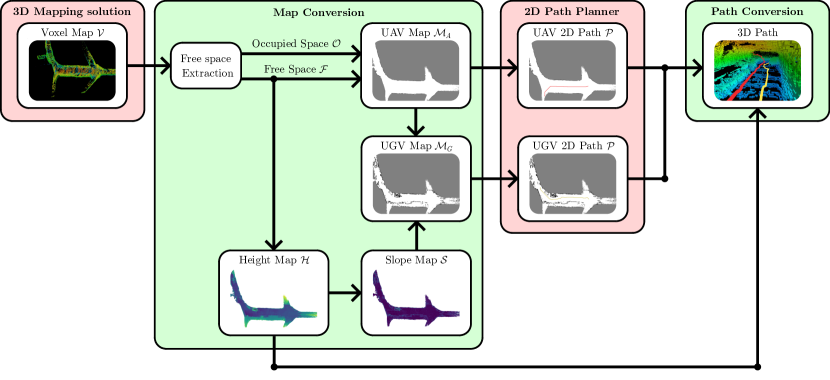
Figure 1: An overview of the proposed methodology for 3D Voxel map to 2D map conversion, along with path planning for the UAVs and UGVs, and 2D to 3D path conversion.

II Problem Formulation

The primary goal of this article is to convert a voxel-based 3D map into a 2D occupancy map, enhanced with height and slope information. This information is vital for path planning in UAVs and UGVs. Additionally, we utilize the 2D occupancy map to generate 3D paths for both aerial and ground robots. This involves transforming paths planned on the output 2D maps, which are produced by the proposed method using a 2D planner, into 3D paths. The map conversions consider whether the robot is aerial or terrestrial. Specifically, for UGVs, slopes that are too steep for traversal will be marked as occupied on the map. The methodology proposed in the article for map conversion is primarily designed for 3D maps produced by UFOMaps[15] but is compatible and generalizable to any voxel-based mapping solution that categorizes space as occupied, free, and unknown. Additionally, the method assumes that the 3D map does not contain multiple levels, such as a map of a single floor of a building or a cave with no overlapping paths.

III 3D to 2D Map Conversion

An overview of the proposed methodology for 3D Voxel map to 2D map conversion is presented in Figure 1. Using the 3D voxel map $\mathcal{V}$, four 2D grid-based maps are generated. Firstly, a height map $\mathcal{H}$ is created, where every cell of a 2D grid map contains height data of the navigable free space relative to the origin of the Voxel map. Secondly, a slope map $\mathcal{S}$ is generated from the height map by estimating the slope of the floor plane in the immediate neighborhood of every cell. Finally, two occupancy maps $\mathcal{M}_{A}$ and $\mathcal{M}_{G}$ are produced, one for the UAVs and the other for UGVs respectively, assigning values: $-1$ for unknown cells, and a value in the range $[0,1]$ for the occupancy probability, with $0$ being free, and $1$ being occupied. All 2D maps are generated over a 2D grid $\mathcal{G}_{2D}$ with the same $x$ and $y$ size/extent and resolution $\mathcal{V}_{res}$ as the Voxel map being converted. Details about the individual steps in the methodology are presented next.

III-A Extraction of Free Space and Height Map

Most robots have their LiDAR mounted vertically, often resulting in an incomplete view of the floor. This configuration leads to numerous gaps in the mapped floor area, as can be seen in Figures 4(e) and 4(f) and Figures 5(e) and 5(f). To address this issue, instead of using occupied voxels, the free space is utilized to identify the floor in $\mathcal{V}$.

III-A1 Free and occupied space

To identify the floor, the map $\mathcal{V}$ is first represented as a union of free $(\mathcal{F})$ and occupied $(\mathcal{O})$ ranges on every cell $\{x_{n},y_{n}\}$ in a 2D grid, denoted as $\mathcal{G}_{2D}$. The free space in the 3D map is represented as $\mathcal{F}=\{F_{x_{1},y_{1}},F_{x_{2},y_{2}},\dots,F_{x_{n},y_{n}}\}$, where $F_{x_{n},y_{n}}=\{f_{1},f_{2},\dots,f_{i}\}$, and each $f_{i}$ is a range containing free spaces at 2D grid location $\{x_{n},y_{n}\}$. Each range of free space $f_{i}\in F_{x_{n},y_{n}}$ contains two values, $f_{i}=\{\hat{f}_{i},\check{f}_{i}\}$, where $\hat{f}_{i}$ is the higher and $\check{f}_{i}$ is the lower bound of the range. Similarly, the occupied space is represented as $\mathcal{O}=\{O_{x_{1},y_{1}},O_{x_{2},y_{2}},\dots,O_{x_{n},y_{n}}\}$, where $O_{x_{n},y_{n}}=\{o_{1},o_{2},\dots,o_{i}\}$ is the set of occupied ranges $o_{i}=\{\hat{o}_{i},\check{o}_{i}\}$. The ranges in the set $F_{x_{i},y_{i}}$ and in the set $O_{x_{i},y_{i}}$ cannot overlap or be connected with another range in the same set.

III-A2 Height map

Since a 2D path planning algorithm utilizing the 2D maps generated in this work cannot perform collision checks on the height axis (the $Z$ axis), the proposed method disregards any free range $f_{i}\in\mathcal{F}$ with a height less than the safety margin $R_{maxZ}$, which is dependent on the dimensions of the robot. In other words, an $f_{i}$ is removed if $||f_{i}||<R_{maxZ}$, where $||f_{i}||$ denotes the height of the range. Given the ranges $F_{x_{i},y_{i}}$ and $O_{x_{i},y_{i}}$, the height map $\mathcal{H}=\{h_{x_{1},y_{1}},h_{x_{2},y_{2}},\dots,h_{x_{n},y_{n}}\}$ is built as a collection of height ranges $h_{i}$, one for each cell $\{x_{i},y_{i}\}$, where $h_{i}=\{\hat{h}_{x_{n},y_{n}},\check{h}_{x_{n},y_{n}}\}$. The bottom of the height range $\check{h}_{x_{n},y_{n}}$ contains the height of the floor and $\hat{h}_{x_{n},y_{n}}$ is the height of the ceiling with respect to the origin of the voxel map. The floor of a cell $\{x_{n},y_{n}\}$ in the 2D grid is assumed to be the bottom of the lowest $f_{i}\in F_{x_{n},y_{n}}$, with the corresponding height set to $\check{h}_{x_{n},y_{n}}$, while the top of the same range $f_{i}\in F_{x_{n},y_{n}}$ is assumed to be the ceiling, with the corresponding height set to $\hat{h}_{x_{n},y_{n}}$.

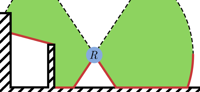
Figure 2: The greedy approach to floor estimation might, in some situations, result in wrongly classifying the floor surface. In this case, the robot $R$ cannot see behind a fence, resulting in the floor (marked by red lines) being identified to be in the air.

Remark 1

As stated in the problem formulation in Section II, the assumption is that there is only one level of navigable space in the map. In environments where there are multiple layers of free space in the height axis, only the lowest free space is used by the method to generate the 2D maps.

The method for free space extraction and height mapping works exceptionally well (as will be presented in Section VI); however, due to its greedy nature, it has drawbacks in some scenarios. Figure 2 shows one such scenario, where a high fence obstructs the robot’s vision. In such a situation, the method will assume that the bottom of the visible parts is the floor, resulting in a perceived connected ’roof’ on the height map connected to the fence. Similarly, places at the edges of the lidar range will be considered as the floor.

III-B Derivation of the Slope Map through Least Squares

The slope map, denoted as $\mathcal{S}=\{s_{x_{1},y_{1}},\dots,s_{x_{n},y_{n}}\}$, is a 2D grid where each cell, represented as $s_{x_{i},y_{i}}$, contains an estimate of the slope of the floor in a neighborhood of the cell. The slope at cell $s_{x_{i},y_{i}}$ is estimated as the slope of the plane fitted using the height and position information of the cells in the height map $\mathcal{H}$ at the same position as $s_{x_{i},y_{i}}$. The cells $h_{x_{j},y_{j}}$ that satisfy the condition $\max(|x_{j}-x_{i}|,|y_{j}-y_{i}|)\leq 1$ are considered as neighbours of the cell $s_{x_{i},y_{i}}$. To fit a plane at the cell $s_{x_{i},y_{i}}$, the linear equation of the form

$$ax+by+c=z$$ (1)

is considered, where the parameters $a$, $b$ and $c$ are real numbers. The interest here is in finding the slope of a plane that is a best fit for the height and position of the cells neighboring the cell $s_{x_{i},y_{i}}$, that is

$$\underbrace{\begin{bmatrix}x_{j_{1}}&y_{j_{1}}&1\\ x_{j_{2}}&y_{j_{2}}&1\\ \vdots&\vdots&\vdots\end{bmatrix}}_{A}\begin{bmatrix}a\\ b\\ c\end{bmatrix}=\underbrace{\begin{bmatrix}\check{h}_{x_{j_{1}},y_{j_{1}}}\\ \check{h}_{x_{j_{2}},y_{j_{2}}}\\ \vdots\end{bmatrix}.}_{B}\\$$ (2)

The parameters of the best-fit plane are found using the least squares method, given by:

$$\begin{bmatrix}a_{ls}\\ b_{ls}\\ c_{ls}\end{bmatrix}=(A^{T}A)^{-1}A^{T}B.$$ (3)

Given Equation (1), the slope at cell $s_{x_{i},y_{i}}$ is given by Equation (4), where $a$ is the slope in the $x$ axis and $b$ is the slope in the $y$ axis.

$$s_{x_{n},y_{n}}=\sqrt{a_{ls}^{2}+b_{ls}^{2}}\text{.}$$ (4)

III-C Generation of 2D Occupancy Maps for UAVs and UGVs

Two occupancy maps $\mathcal{M}=\{m_{x_{1},y_{1}},\dots,m_{x_{n},y_{n}}\}$ are constructed: one for UAVs, $\mathcal{M}_{A}$ and the other for UGVs, $\mathcal{M}_{G}$.

III-C1 UAV map $\mathcal{M}_{A}$

The map generation begins by representing all cells of the 2D occupancy maps with free space identified in subsection III-A as free, i.e., $m_{x_{n},y_{n}}=0$, when $F_{x_{j},y_{j}}\neq\{\varnothing\}$. The remaining cells $m_{x_{j},y_{j}}$ that are not free, but have at least one neighboring cell that is free are examined using the following criteria to decide their occupancy probabilities:

$$m_{x_{j},y_{j}}=\left\{\begin{matrix}O_{cc}(x_{j},y_{j})\;&\text{if}\;O_{cc}(x_{j},y_{j})<O_{min}\\ -1\;&\text{else}\end{matrix}\right.$$ (5)

where $O_{cc}(x_{j},y_{j})$ is the occupancy value in the range $0$ and $1$ for the examined map cell $m_{x_{j},y_{j}}$ and $O_{min}$ is the minimum allowed occupancy value. The function of $O_{cc}(x_{j},y_{j})$ is defined in Equation (6) and calculates the overlapping percentage between the occupied ranges of $O_{x_{j},y_{j}}$ and the neighboring free space in the height map $\mathcal{H}$.

$$O_{cc}(x_{j},y_{j})=\max_{{x_{k},y_{k}}\in N(x_{j},y_{j})}\left(\frac{\sum_{o_{i}\in O_{x_{j},y_{j}}}k(h_{x_{k},y_{k}},o_{i})}{||h_{x_{k},y_{k}}||}\right)$$ (6)

where the function $k(f_{x_{n},y_{n}},o_{x_{n},y_{n}})$ is defined as:

$$\begin{matrix}k(h_{x_{n},y_{n}},o_{i})=\max(0,\min(\hat{h}_{x_{n},y_{n}},\hat{o}_{i})-\max(\check{h}_{x_{n},y_{n}},\check{o}_{i}))\end{matrix}$$ (7)

The function $k(h_{x_{n},y_{n}},o_{i})$ returns the length of the overlap between the two ranges, and when there is no overlap, the function returns $0$. If the examined cell has multiple neighboring free cells, only the free cell that results in the maximum occupancy is used. In Equation (6), $N(x_{1},y_{1})$ is a set of neighboring cells $\{x_{n},y_{n}\}$ with $m_{x_{n},y_{n}}=0$, i.e., the cells containing free navigable range that satisfy the conditions in the following equation:

$$\begin{matrix}N(x_{j},y_{j})=\\ \{x_{n},y_{n}|\max(|x_{n}-x_{j}|,|y_{n}-y_{j}|)=1.m_{x_{n},y_{n}}=0\}.\end{matrix}$$ (8)

Note that low walls and scattered objects are not relevant for aerial robot navigation, as there is navigable space for aerial robots above the walls and scattered objects. The approach proposed for the generation of $\mathcal{M}_{A}$ is concerned with the detection of free space for aerial navigation and ignores such entities for the aerial robot maps.

III-C2 UGV map $\mathcal{M}_{G}$

The 2D map generation for ground-based robots utilizes the same free space and occupancy detection as the map generated for the UAV, but in addition, the slope map generated in subsection III-B is used as well. In the UGV map $\mathcal{M}_{G}$, if the slope associated with a cell that is free is greater than $R_{MS}$, the cell is instead considered occupied, where $R_{MS}$ is the maximum slope a ground robot can climb. Thus, the low walls and scattered objects that are relevant for UGVs are detected and represented in the UGV map $\mathcal{M}_{G}$.

IV Use Cases and Utility of the Method

The authors identify two distinct use cases for the 3D to 2D map conversion method proposed in this work. The first is to minimize computations and memory usage for both UAVs and UGVs in large-scale navigation scenarios, and the second is to reduce the data transmitted between multiple robotic agents in bandwidth-limited scenarios.

In the first case, the 2D maps can be used to find 3D paths for UAVs and UGvs for efficient large-scale navigation. A general path is initially determined for the robots on the 2D map, using any of the classical or state-of-the-art occupancy-grid-based path planning methods, followed by elevation of the path into 3D space through the approach described in section V. Path planning using the 2D map is more efficient with respect to memory and CPU usage. This, as a 2D map, is significantly lighter on memory, and navigation problems are quicker to solve, as the $Z$-axis need not be considered. For very precise local navigation, a local section of the voxel map in a small neighborhood of the robot can be used, as there is no necessity to load the complete voxel map. This strategy also allows the robot to maintain a higher-resolution local voxel map, as it only needs to store a small portion of the complete map in its memory.

The second case addresses scenarios where multiple robotic agents need to communicate and exchange local sections of a larger map with each other. Since the 2D map generally has a smaller file size, it can be transmitted between robots more rapidly within the allocated bandwidth. Although the 2D map, along with the height map, does not perfectly represent the environment, it still offers a good practical sense of the layout, enabling the robots to perform general path planning, as stated previously.

V 2D to 3D Path Conversion

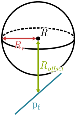
Figure 3: A sphere-shaped safety region is used to find collision-free paths for the UAVs.

As discussed in Section IV, one of the primary advantages of the proposed method is its ability to plan paths using a 2D map instead of relying on a full 3D voxel map. Let us assume that a classical or state-of-the-art 2D path planner is used to find paths in the UAV and UGV maps. To make the 2D paths practicable for robots, especially UAVs, it is essential to determine the height, the $Z$ position, of each point along the path. To address this challenge, the following process is employed to determine the $Z$ position of each point on a 2D path $\mathcal{P}$ generated on the 2D occupancy maps.

To determine the height $\mathcal{P}_{iZ}$ of each point $\mathcal{P}_{i}$ on the path $\mathcal{P}$, the following equation is used:

$$\mathcal{P}_{iZ}=\max\left(\check{\mathcal{H}}(\mathcal{P}_{i-p_{f}}),\dots,\check{\mathcal{H}}(\mathcal{P}_{i+p_{f}})\right)+R_{off}$$ (9)

where $\check{\mathcal{H}}(\mathcal{P}_{i})$ represents the floor height in the height map $\mathcal{H}$ at the position of $\mathcal{P}_{i}$. The parameter $p_{f}$ is user-defined, specifying the number of steps that are considered in front of and behind the robot along the path. The $R_{off}$ is another user-defined parameter that sets a desired safe height above the ground for the path. The use of the $\max$ function ensures that the path adjusts its height $p_{f}$ steps before encountering an obstacle. For generating 3D paths for the UAVs, an additional check is performed to avoid collisions with the safety region around the robot. The method uses a sphere-shaped safety region for UAVs, as illustrated in Figure 3. The safety region has a radius of $0<R_{r}\leq 2*R_{maxZ}$. If the height calculated in the previous step results in a collision with either the floor or the ceiling in the height map $\mathcal{H}$, the point in the path that results in a collision is moved to a $Z$ position that will not cause a collision, ignoring $R_{off}$ at that point in the path.

VI Validation

The proposed method was validated in two environments: a cave environment and an indoor environment. A voxel map was generated with a resolution of $\mathcal{V}_{res}=0.1$ m in the cave environment and with a resolution of $\mathcal{V}_{res}=0.05$ in the indoor environment. Using the map conversion method outlined in Section III, 2D occupancy maps $\mathcal{M}_{A}$ and $\mathcal{M}_{G}$ were generated from voxel maps of the two environments. The 2D maps for the Unmanned Aerial Vehicle (UAV) are shown in Figures 4(a) and 5(a), and for the Unmanned Ground Vehicle (UGV) are shown in Figures 4(b) and 5(b). Note that low walls and scattered objects are not relevant for aerial robots, as there is navigable space for aerial robots above the walls and scattered objects. For the ground robots, however, the walls and scattered objects are highly relevant and are retained by the proposed method, using the information contained in the slope map (the procedure is described in Section III-C).

The height map $\mathcal{H}$, specifically $\check{h}_{x_{i},y_{i}}$, is utilized to find the floor and the ceiling of the map. The height of the floor, with respect to the origin of the voxel map, is depicted in Figures 4(c) and 5(c). Using the height maps, slope estimation described in Section III-B is used to find the slope in the neighborhood of every grid cell. The slope maps are depicted in Figures 4(d) and 5(d). The slope maps, along with the UAV maps, are used to find the 2D occupancy maps for the ground robots, which are shown in Figures 4(b) and 5(b). In the slope map, the boundary of low walls and obstacles can clearly be seen. In the UAV maps, the slope thresholding approach using the parameter $R_{MS}$ (described in Section III-C) is used to assign the cells associated with the boundaries of walls and scattered objects an occupancy value of 1. Two 2D paths were generated using a 2D planning algorithm: one for the Unmanned Aerial Vehicle (UAV), as shown in Figures 4(a) and 5(a), and another for the Unmanned Ground Vehicle (UGV), as seen in Figures 4(b) and 5(b). The 3D paths for both robots are generated using the method in V, as shown in the figures 4(e), 4(f), 5(e), and 5(f). The parameters used in 3D to 2D map conversion and for 3D path generation are listed in Table I.

TABLE I: Parameters used in the validation cases.

	$R_{maxZ}$	$O_{max}$	$R_{MS}$	$R_{r}$	$R_{off}$	$p_{f}$
UAV	1 m	0.1	NA	0.5 m	1 m	1 m / $\mathcal{V}_{res}$
UGV	1 m	0.1	0.35	NA	0.1 m	1 m / $\mathcal{V}_{res}$

VII Discussion

As demonstrated in Section VI, the method effectively converts voxel maps in environments featuring non-uniform height variations and in the presence of overhangs/ceilings. The UGV map includes obstacles and walls impassable by the UGV, thus ensuring comprehensive environmental representation. However, a limitation of the traversability slope estimation discussed in Section III-B is its dependency on having a sufficiently low resolution in the voxel map. In the validation of the proposed method, a resolution of $\mathcal{V}_{res}=0.1$ m and $\mathcal{V}_{res}=0.05$ was utilized, which is relatively fine for voxel mapping. Nonetheless, as argued in Section IV, by using a 2D map for global navigation, only a small local portion of the 3D map is needed for local navigation. This allows the local map to have a higher resolution without significant memory cost compared to needing to have the full voxel map loaded.

A further issue with the UGV map is the inaccurate representation at some frontiers, which form the boundary between free and unknown space. This inaccuracy arises from the 3D mapping solutions, which do not map the floor correctly at the edges of the Lidar. Thus, the greedy method for free-space detection presented in Section III-A results in a sudden height increase in the area near the frontiers. Despite this limitation, the mapped area remains accurate for UGV navigation. In scenarios such as autonomous exploration, reliable frontier detection is an absolute necessity. The limitation implies that the UGV-generated map is unsuitable in the exploration case, thus necessitating reliance on the local voxel map for frontier detection.

One limitation of using a 2D planner for UAV path planning instead of a full 3D planner is that it overlooks height variations in the environment. While this may not be problematic in general, this limitation can lead to suboptimal path choices, as circumventing a tall obstacle might be more efficient than flying over it. A potential solution could be to integrate height differences into the 2D planner’s calculations, thus utilizing the height map produced by the method more effectively, and this would form one of our future research directions.

VIII Conclusions

Motivated by the expensive cost of UAV and UGV navigation planning over large-scale 3D maps, both in terms of CPU and memory, this work presented a novel method for converting 3D voxel maps to 2D occupancy maps for ground and aerial robots, along with an accompanying height map. By allowing the robots to use a 2D map for large-scale navigation, CPU usage can be minimized by using computationally efficient 2D planners instead of full 3D planners. This, combined with the fact that a 2D map uses less memory than a 3D map, results in a more computationally efficient large-scale navigation stack for an autonomous robot. A method was also proposed for converting the paths generated by the 2D planer back into 3D space using the height information extracted by the method. The method proposed in this paper is capable of generating 3D paths for both ground and aerial robots and was validated successfully in two different environments (a cave and an indoor scenario).

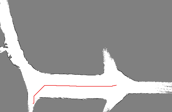
(a) UAV map and path plan for a UAV

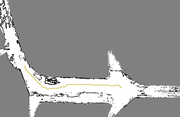
(b) UGV map and path plan for a UGV

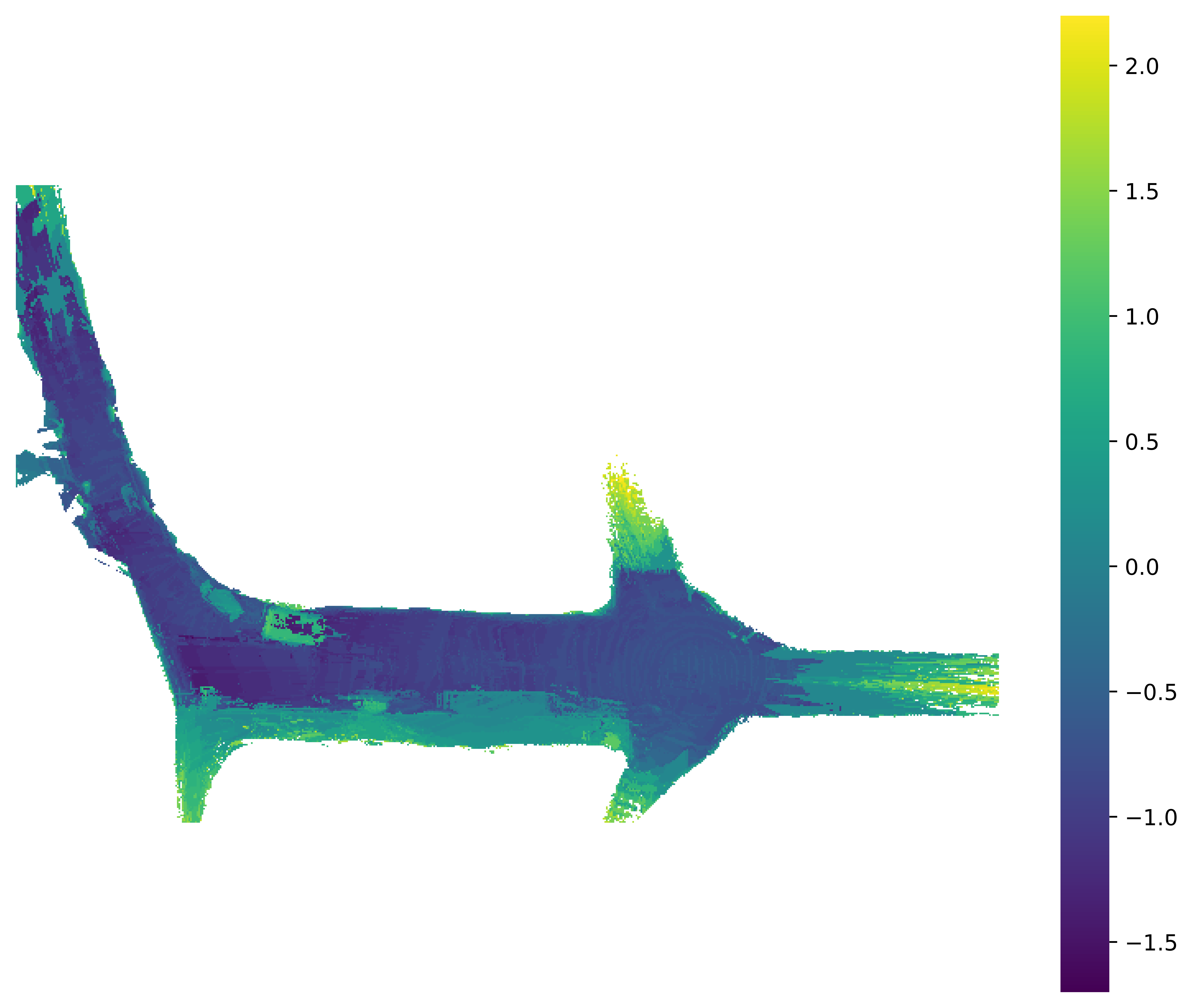
(c) Height map

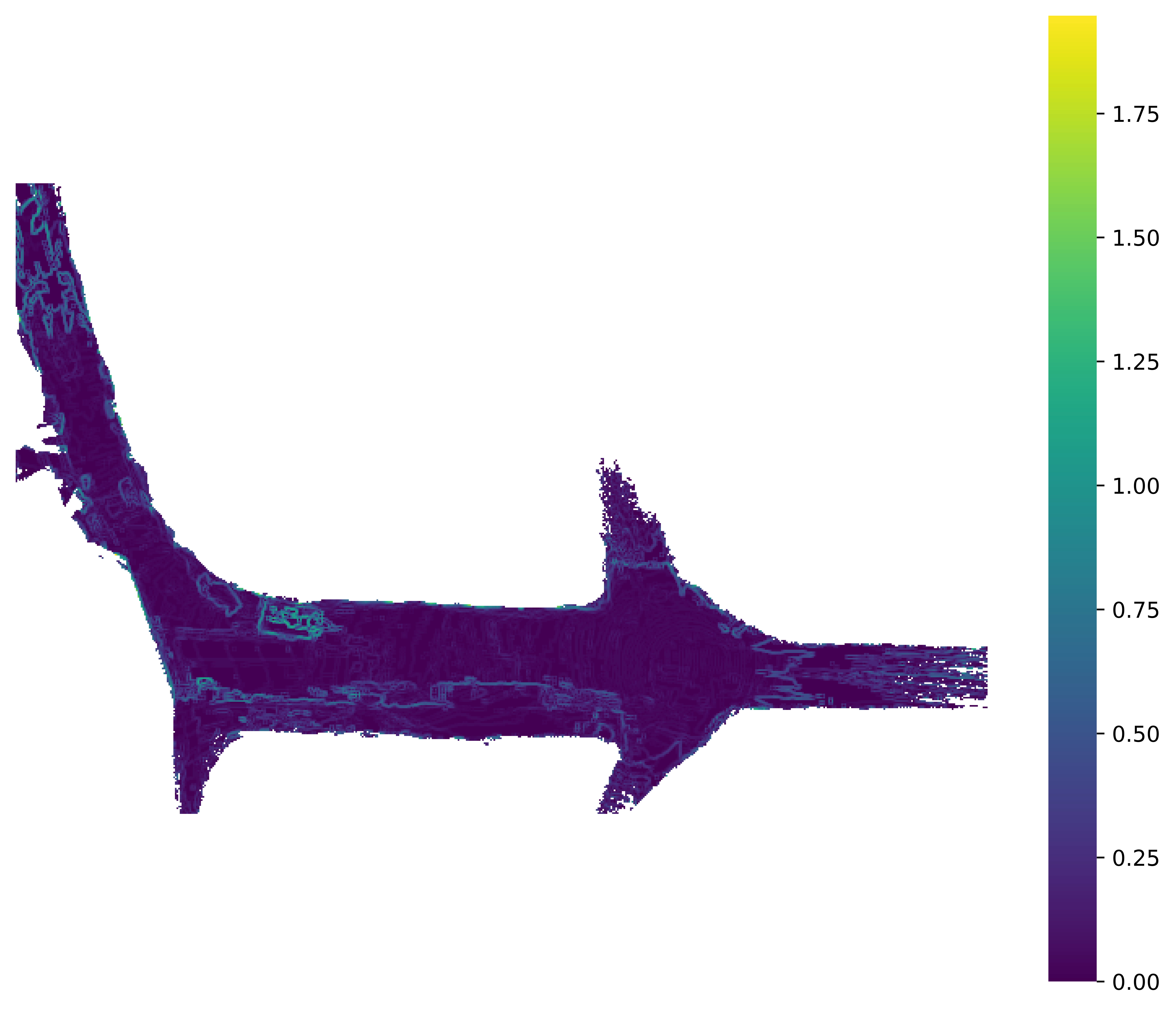
(d) Slope map

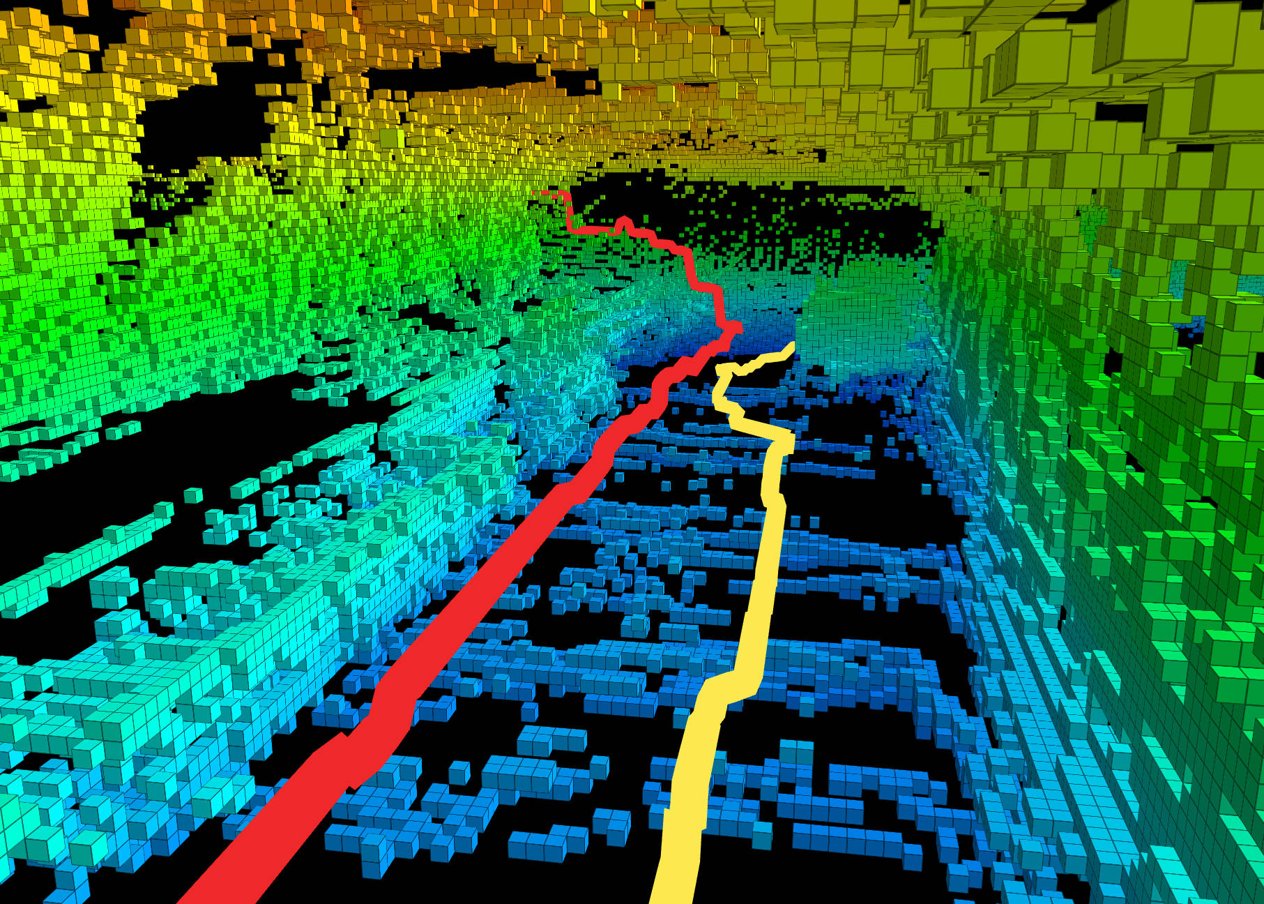
(e) Voxel map perspective 1 with 3D paths for UAV (red) and UGV (yellow).

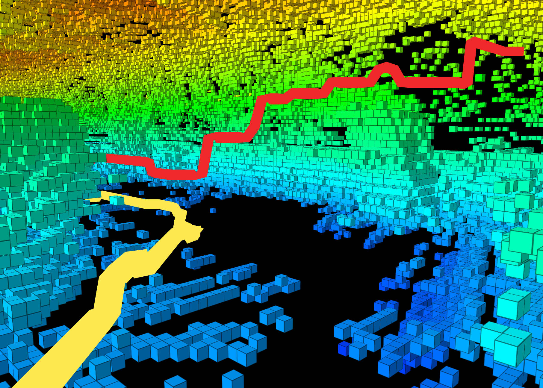
(f) Voxel map perspective 2 with 3D paths for UAV (red) and UGV (yellow).

Figure 4: 2D maps and paths generated by the proposed methods for UAV and UGV in the cave environment. The results from the 2D path to 3D path conversion are shown in subfigures e) and f).

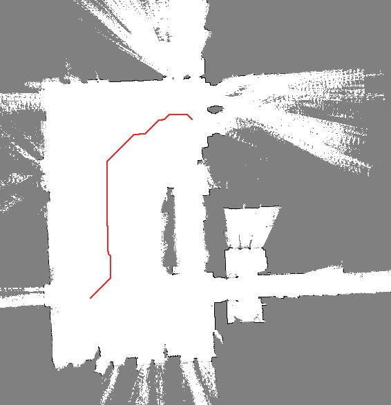
(a) UAV map and path plan for a UAV

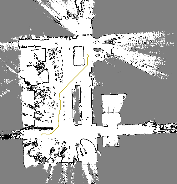
(b) UGV map and path plan for a UGV

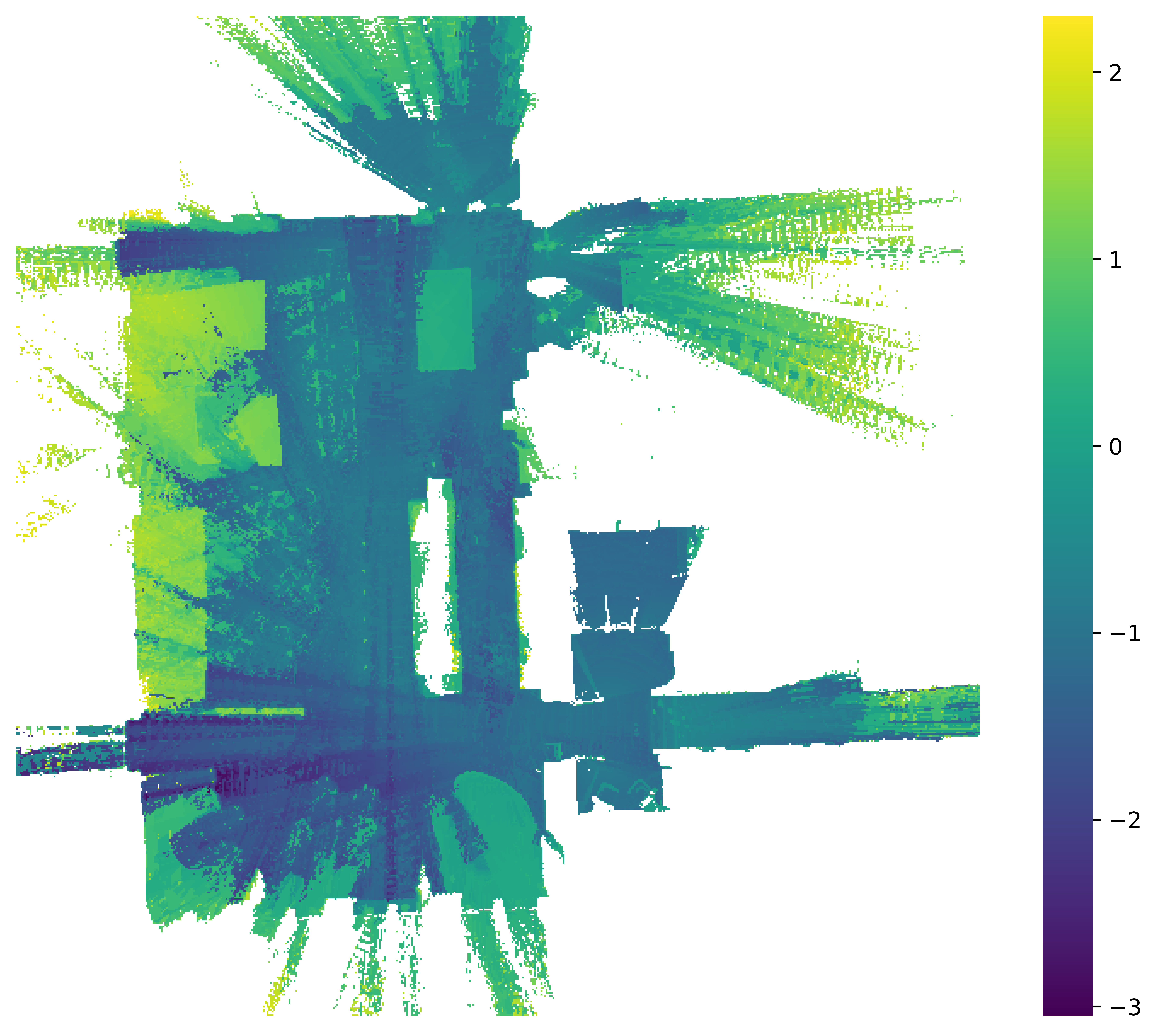
(c) Height map

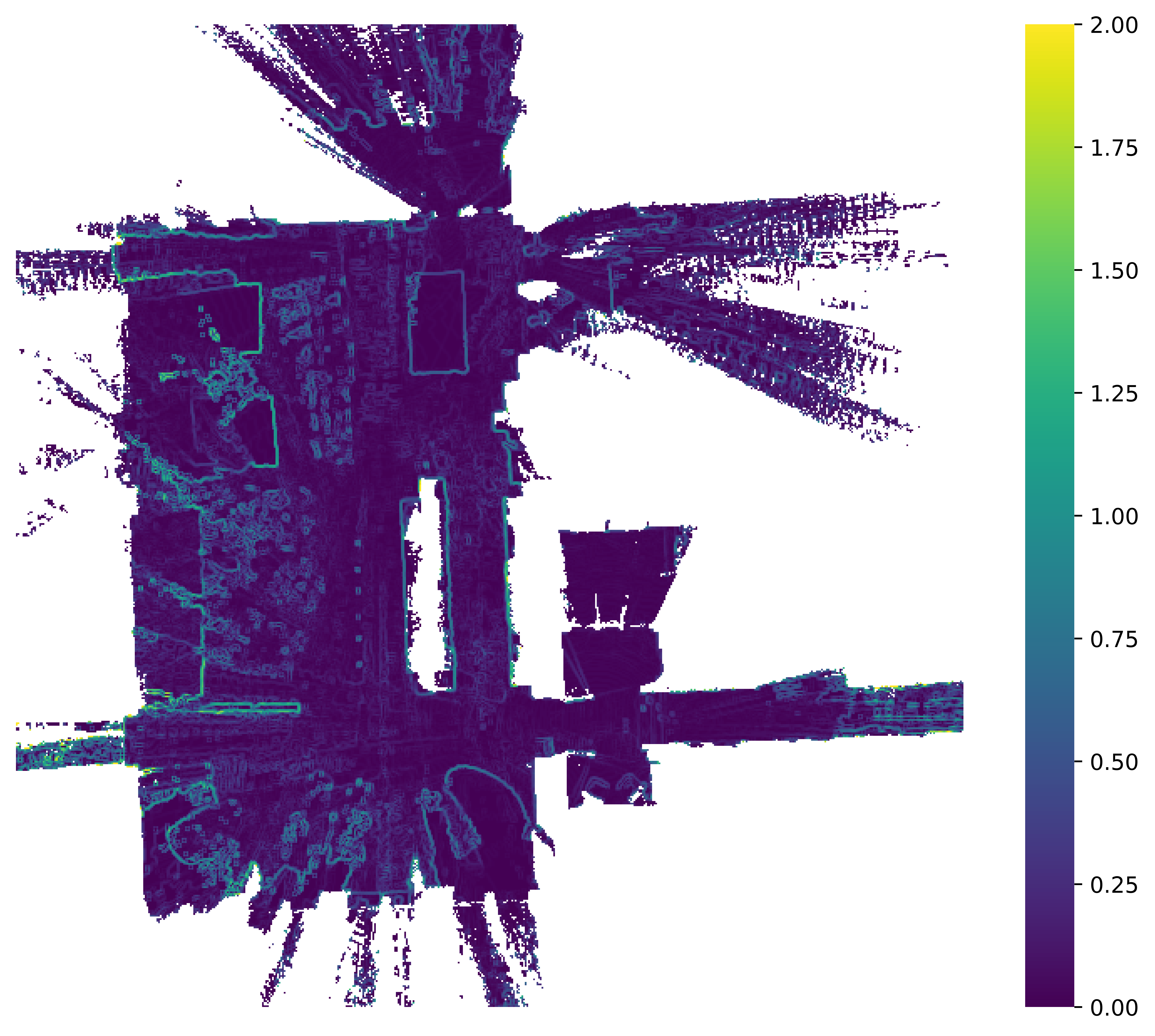
(d) Slope map

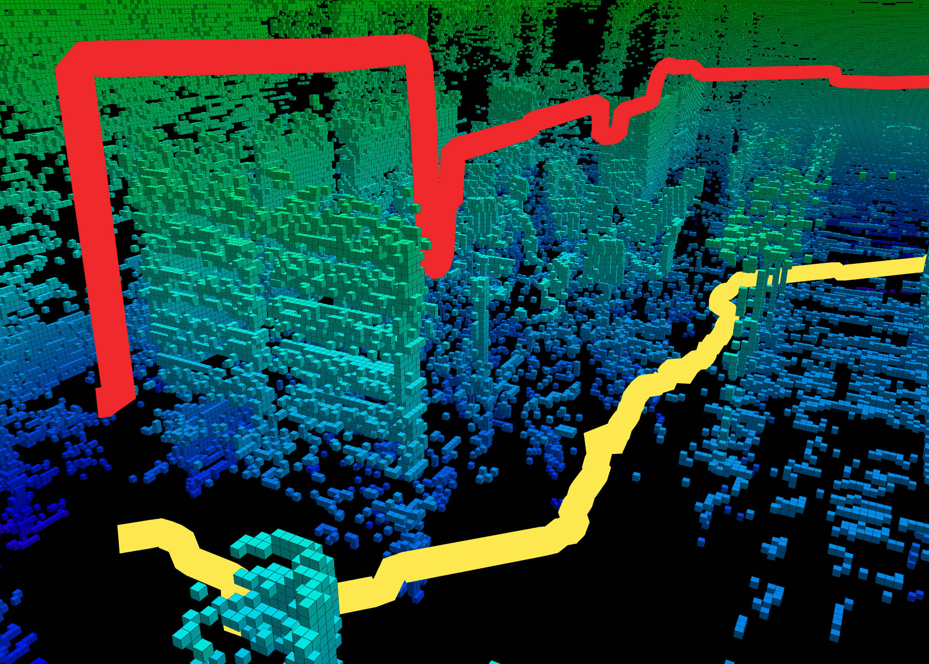
(e) Voxel map perspective 1 with 3D paths for UAV (red) and UGV (yellow).

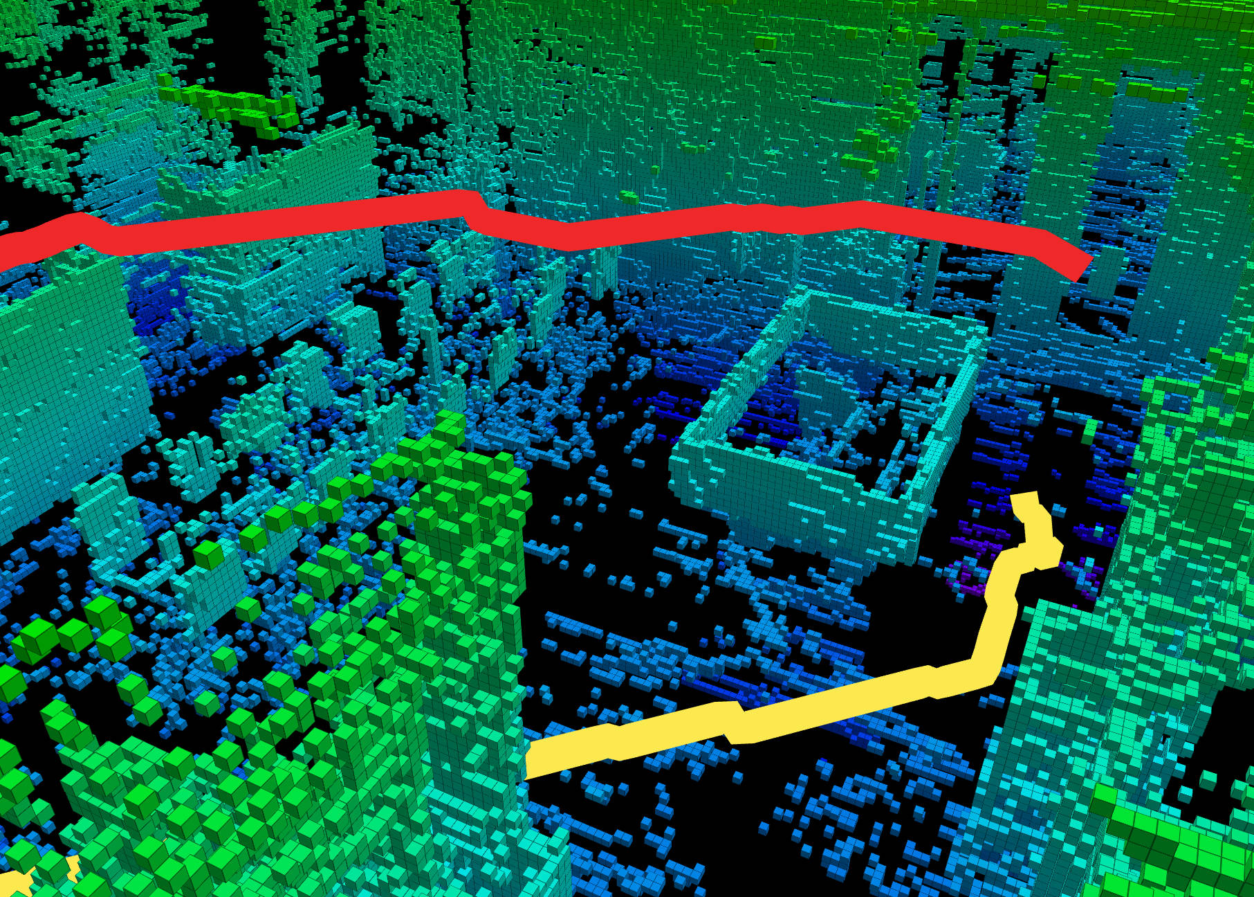
(f) Voxel map perspective 2 with 3D paths for UAV (red) and UGV (yellow).

Figure 5: 2D maps and paths generated by the proposed methods for UAV and UGV in the cave environment. The results from the 2D path to 3D path conversion are shown in subfigures e) and f).

References

- [1] R. K. Megalingam, S. Tantravahi, H. S. S. K. Tammana, and H. S. R. Puram, “2D-3D hybrid mapping for path planning in autonomous robots,” International Journal of Intelligent Robotics and Applications, vol. 7, no. 2, pp. 291–303, June 2023.
- [2] O. Wulf, K. Arras, H. Christensen, and B. Wagner, “2D mapping of cluttered indoor environments by means of 3D perception,” in IEEE International Conference on Robotics and Automation, 2004. Proceedings. ICRA ’04. 2004, vol. 4, Apr. 2004, pp. 4204–4209 Vol.4, iSSN: 1050-4729.
- [3] S. Sandfuchs, M. P. Heimbach, J. Weber, and M. Schmidt, “Conversion of depth images into planar laserscans considering obstacle height for collision free 2D robot navigation,” in 2021 European Conference on Mobile Robots (ECMR), Aug. 2021, pp. 1–6. [Online]. Available: https://ieeexplore.ieee.org/document/9568795
- [4] A. Mora, R. Barber, and L. Moreno, “Leveraging 3D Data for Whole Object Shape and Reflection Aware 2D Map Building,” IEEE Sensors Journal, pp. 1–1, 2023.
- [5] T. H. Nam, J. H. Shim, and Y. I. Cho, “A 2.5D Map-Based Mobile Robot Localization via Cooperation of Aerial and Ground Robots,” Sensors, vol. 17, no. 12, p. 2730, Dec. 2017.
- [6] A. Hornung, K. M. Wurm, M. Bennewitz, C. Stachniss, and W. Burgard, “OctoMap: an efficient probabilistic 3D mapping framework based on octrees,” Autonomous Robots, vol. 34, no. 3, pp. 189–206, Apr. 2013.
- [7] S. Yang, S. Yang, and X. Yi, “An Efficient Spatial Representation for Path Planning of Ground Robots in 3D Environments,” IEEE Access, vol. 6, pp. 41 539–41 550, 2018.
- [8] Y. Li, D. Wang, Q. Li, G. Cheng, Z. Li, and P. Li, “Advanced 3D Navigation System for AGV in Complex Smart Factory Environments,” Electronics, vol. 13, no. 1, p. 130, Jan. 2024.
- [9] K. Kamarudin, S. M. Mamduh, A. Y. M. Shakaff, S. M. Saad, A. Zakaria, A. H. Abdullah, and L. M. Kamarudin, “Method to convert Kinect’s 3D depth data to a 2D map for indoor SLAM,” in 2013 IEEE 9th International Colloquium on Signal Processing and its Applications, Mar. 2013, pp. 247–251.
- [10] L. Garrote, J. Rosa, J. Paulo, C. Premebida, P. Peixoto, and U. J. Nunes, “3D point cloud downsampling for 2D indoor scene modelling in mobile robotics,” in 2017 IEEE International Conference on Autonomous Robot Systems and Competitions (ICARSC), Apr. 2017, pp. 228–233.
- [11] G. Brahmanage and H. Leung, “Building 2D Maps with Integrated 3D and Visual Information using Kinect Sensor,” in 2019 IEEE International Conference on Industrial Cyber Physical Systems (ICPS), May 2019, pp. 218–223.
- [12] A. Yusefi, A. Durdu, and C. Sungur, “ORB-SLAM-based 2D Reconstruction of Environment for Indoor Autonomous Navigation of UAVs,” Avrupa Bilim ve Teknoloji Dergisi, pp. 466–472, Oct. 2020.
- [13] R. Mur-Artal, J. M. M. Montiel, and J. D. Tardós, “ORB-SLAM: A Versatile and Accurate Monocular SLAM System,” IEEE Transactions on Robotics, vol. 31, no. 5, pp. 1147–1163, Oct. 2015.
- [14] H. Gim, M. Jeong, and S. Han, “Autonomous Navigation System with Obstacle Avoidance using 2.5D Map Generated by Point Cloud,” in 2021 21st International Conference on Control, Automation and Systems (ICCAS), Oct. 2021, pp. 749–752, iSSN: 2642-3901.
- [15] D. Duberg and P. Jensfelt, “UFOMap: An Efficient Probabilistic 3D Mapping Framework That Embraces the Unknown,” IEEE Robotics and Automation Letters, vol. 5, no. 4, pp. 6411–6418, Oct. 2020.