Infinite-Horizon Distributionally Robust Regret-Optimal Control

Abstract

We study the infinite-horizon distributionally robust (DR) control of linear systems with quadratic costs, where disturbances have unknown, possibly time-correlated distribution within a Wasserstein-2 ambiguity set. We aim to minimize the worst-case expected regret—the excess cost of a causal policy compared to a non-causal one with access to future disturbance. Though the optimal policy lacks a finite-order state-space realization (i.e., it is non-rational), it can be characterized by a finite-dimensional parameter. Leveraging this, we develop an efficient frequency-domain algorithm to compute this optimal control policy and present a convex optimization method to construct a near-optimal state-space controller that approximates the optimal non-rational controller in the $\mathit{H}_{\infty}$-norm. This approach avoids solving a computationally expensive semi-definite program (SDP) that scales with the time horizon in the finite-horizon setting.

1 Introduction

Addressing uncertainty is a core challenge in decision-making. Control systems inherently encounter various uncertainties, such as external disturbances, measurement errors, model disparities, and temporal variations in dynamics (van der Grinten, 1968; Doyle, 1985). Neglecting these uncertainties in policy design can result in considerable performance decline and may lead to unsafe and unintended behavior (Samuelson & Yang, 2017).

Traditionally, the challenge of uncertainty in control systems has been predominantly approached through either stochastic or robust control frameworks (Kalman, 1960; Zames, 1981; Doyle et al., 1988). Stochastic control (e.g., Linear–Quadratic–Gaussian (LQG) or $H_{2}$-control) aims to minimize an expected cost, assuming disturbances follow a known probability distribution (Hassibi et al., 1999). However, in practical scenarios, the true distribution is often estimated from sampled data, introducing vulnerability to inaccurate models. On the other hand, robust control minimizes the worst-case cost across potential disturbance realizations, such as those with bounded energy or power ($H_{\infty}$ control) (Zhou et al., 1996). While this ensures robustness, it can be overly conservative. Two recent approaches have emerged to tackle this challenge.

Regret-Optimal (RO) Control. Introduced by (Sabag et al., 2021; Goel & Hassibi, 2023), this framework offers a promising strategy to tackle both stochastic and adversarial uncertainties. It defines regret as the performance difference between a causal control policy and a clairvoyant, non-causal one with perfect knowledge of future disturbances. In the full-information setting, RO controllers minimize the worst-case regret across all bounded energy disturbances (Sabag et al., 2021; Goel & Hassibi, 2023). The infinite-horizon RO controller also takes on a state-space form, making it conducive to efficient real-time computation (Sabag et al., 2021).

Extensions of this framework have been investigated in various settings, including measurement-feedback control (Goel & Hassibi, 2021a; Hajar et al., 2023b), dynamic environments (Goel & Hassibi, 2021b), safety-critical control (Martin et al., 2022; Didier et al., 2022), filtering (Sabag & Hassibi, 2022; Goel & Hassibi, 2023), and distributed control (Martinelli et al., 2023). While these controllers effectively emulate the performance of non-causal controllers in worst-case disturbance scenarios, they may exhibit excessive conservatism when dealing with stochastic ones.

Distributionally Robust (DR) Control. In contrast to traditional approaches such as $H_{2}$ or $H_{\infty}$ and RO control that focus on a single distribution or worst-case disturbance realization, the DR framework addresses uncertainty in disturbances by considering ambiguity sets – sets of plausible probability distributions (Yang, 2020; Kim & Yang, 2023; Hakobyan & Yang, 2022; Taskesen et al., 2023; Aolaritei et al., 2023a, b; Brouillon et al., 2023). This methodology aims to design controllers with robust performance across all probability distributions within a given ambiguity set. The size of the ambiguity set provides control over the desired robustness against distributional uncertainty, ensuring that the resulting controller is not excessively conservative.

The controller’s performance is highly sensitive to the chosen metric for quantifying distributional shifts. Common choices include the total variation (TV) distance (Tzortzis et al., 2015, 2016), the Kullback-Leibler (KL) divergence (Falconi et al., 2022; Liu et al., 2023), and the Wasserstein-2 ($\mathsf{W_{2}}$) distance (Taha et al., 2023; Taskesen et al., 2023; Aolaritei et al., 2023a; Hajar et al., 2023a; Brouillon et al., 2023; Kargin et al., 2023). The controllers derived from KL-ambiguity sets (Petersen et al., 2000; Falconi et al., 2022) have been linked to the well-known risk-sensitive controller (Jacobson, 1973; Speyer et al., 1974; Whittle, 1981), which minimizes an exponential cost (see (Hansen & Sargent, 2008) and the references therein). However, distributions in a KL-ambiguity set are restricted to be absolutely continuous with respect to the nominal distribution (Hu & Hong, 2012), significantly limiting its expressiveness.

In contrast, $\mathsf{W_{2}}$-distance, which quantifies the minimal cost of transporting mass between two probability distributions, induces a Riemannian structure on the space of distributions (Villani, 2009) and allows for ambiguity sets containing distributions with both discrete and continuous support. Thanks to this versatility and the rich geometric framework, it has found widespread adoption across various fields, including machine learning (Arjovsky et al., 2017), computer vision (Liu et al., 2020; Ozaydin et al., 2024), estimation and filtering (Shafieezadeh Abadeh et al., 2018; Lotidis et al., 2023; Prabhat & Bhattacharya, 2024), data compression (Blau & Michaeli, 2019; Lei et al., 2021; Malik et al., 2024), and robust optimization (Zhao & Guan, 2018; Kuhn et al., 2019; Gao & Kleywegt, 2022; Blanchet et al., 2023). Moreover, the $\mathsf{W_{2}}$-distance has emerged as a theoretically appealing statistical distance for DR linear-quadratic control problems (Taha et al., 2023) due to its compatibility with quadratic objectives and the resulting tractability of the associated optimization problems (Gao & Kleywegt, 2022).

1.1 Contributions

This paper explores the framework of Wasserstein-2 distributionally robust regret-optimal (DR-RO) control of linear dynamical systems in the infinite-horizon setting. Initially introduced by (Taha et al., 2023) for the full-information setting, DR-RO control was later adapted to the partially observable case by (Hajar et al., 2023a). Similarly, (Taskesen et al., 2023) derived a DR controller for the partially observed linear-quadratic-Gaussian (LQG) problem, assuming time-independent disturbances. These prior works, focusing on the finite-horizon setting, are hampered by the requirement to solve a semi-definite program (SDP) whose complexity scales with the time horizon, prohibiting their applicability for large horizons.

Our work addresses this limitation by considering the infinite-horizon setting where the probability distribution of the disturbances over the entire time horizon is assumed to lie in a $\mathsf{W_{2}}$-ball of a specified radius centered at a given nominal distribution. We seek a linear time-invariant (LTI) controller that minimizes the worst-case expected regret for distributions adversarially chosen within the $\mathsf{W_{2}}$-ambiguity set. Our contributions are summarized as follows.

1. Stabilizing time-invariant controller. As opposed to the finite-horizon controllers derived in (Hakobyan & Yang, 2022; Taskesen et al., 2023; Aolaritei et al., 2023b; Taha et al., 2023; Hajar et al., 2023a), the controllers obtained in the infinite-horizon setting stabilize the underlying dynamics (Corollary 3.4)

2. Robustness against non-iid disturbances. In contrast to several prior works that assume time-independence of disturbances (Yang, 2020; Kim & Yang, 2023; Hakobyan & Yang, 2022; Taskesen et al., 2023; Zhong & Zhu, 2023; Aolaritei et al., 2023a, b), our approach does not impose such assumptions, thereby ensuring that the resulting controllers are robust against time-correlated disturbances.

3. Characterization of the optimal controller. We cast the DR-RO control problem as a max-min optimization and derive the worst-case distribution and the optimal controller using KKT conditions (Theorem 3.2). While the resulting controller is non-rational, lacking a finite-order state-space realization (Corollary 4.3), we show it admits a finite-dimensional parametric form (Theorem 4.2).

4. Efficient computation of the optimal controller. Utilizing the finite-dimensional parametrization, we propose an efficient algorithm based on the Frank-Wolfe method to compute the optimal non-rational DR-RO controller in the frequency-domain with arbitrary fidelity (Algorithm 1).

5. Near-optimal state-space controller. We introduce a novel convex program that finds the best rational approximation of any given order for the non-rational controller in the $\mathit{H}_{\infty}$-norm (Theorem 5.5). Therefore, our approach enables efficient real-time implementation using a near-optimal state-space controller (Lemma 5.7).

Notations: The letters $\mathbb{N}$, $\mathbb{Z}$, $\mathbb{R}$, and $\mathbb{C}$ denote the set of natural numbers, integers, real, and complex numbers, respectively. $\mathbb{T}$ denotes the complex unit circle. For $z\!\in\!\mathbb{C}$, $|{z}|$ is its magnitude, and $z^{\ast}$ is the conjugate. $\mathbb{S}_{+}^{n}$ denotes the set of positive semidefinite (psd) matrices of size $n\!\times\!n$. Bare calligraphic letters ($\mathcal{K}$, $\mathcal{M}$, etc.) are reserved for operators. $\mathcal{I}$ is the identity operator with a suitable block size. For an operator $\mathcal{M}$, its adjoint is $\mathcal{M}^{\ast}$. For a matrix $A$, its transpose is $A^{\intercal}$, and its Hermitian conjugate is $A^{\ast}$. For psd operators/matrices, $\succcurlyeq$ denotes the Loewner order. For a psd operator $\mathcal{M}$, both $\sqrt{\mathcal{M}}$ and $\mathcal{M}^{\frac{1}{2}}$ denote the PSD square-root. $\{\mathcal{M}\}_{+}$ and $\{\mathcal{M}\}_{-}$ denote the causal and strictly anti-causal parts of an operator $\mathcal{M}$. $M(z)$ denotes the z-domain transfer function of a Toeplitz operator $\mathcal{M}$. $\operatorname{tr}(\cdot)$ denotes the trace of operators and matrices. $\|{\cdot}\|_{\text{}}$ is the usual Euclidean norm. $\|{\cdot}\|_{\infty}$ and $\|{\cdot}\|_{2}$ are the $\mathit{H}_{\infty}$ operator) and $\mathit{H}_{2}$ (Frobenius) norms, respectively. Probability distributions are denoted by $\operatorname{\mathbb{P}}$. $\mathscr{P}_{p}(\mathbb{R}^{d})$ denotes the set of distributions with finite $p^{\textrm{th}}$ moment over a $\mathbb{R}^{d}$. $\operatorname{\mathbb{E}}$ denotes the expectation. The Wasserstein-2 distance between distributions $\operatorname{\mathbb{P}}_{1},\operatorname{\mathbb{P}}_{2}\!\in\!\mathbb{R}^{d}$ is denoted by $\mathsf{W_{2}}(\operatorname{\mathbb{P}}_{1},\operatorname{\mathbb{P}}_{2})$ such that

$$\mathsf{W_{2}}(\operatorname{\mathbb{P}}_{1},\operatorname{\mathbb{P}}_{2})\triangleq\left({\inf\,\operatorname{\mathbb{E}}\left[{\|{\mathbf{w}_{1}\!-\!\mathbf{w}_{2}}\|_{\text{}}^{2}}\right]}\right)^{1/2},$$ (1)

where the infimum is over all joint distributions of $(\mathbf{w}_{1},\mathbf{w}_{2})$ with marginals $\mathbf{w}_{1}\!\stackrel{{\scriptstyle\text{}}}{{\sim}}\!\operatorname{\mathbb{P}}_{1}$ and $\mathbf{w}_{2}\!\stackrel{{\scriptstyle\text{}}}{{\sim}}\!\operatorname{\mathbb{P}}_{2}$.

2 Preliminaries

2.1 Linear-Quadratic Control

Consider a discrete-time, linear time-invariant (LTI) dynamical system expressed as a state-space model given by:

$$x_{t+1} =Ax_{t}+B_{u}u_{t}+B_{w}w_{t},\quad s_{t}=Cx_{t}.$$ (2)

Here, $x_{t}\!\in\!\mathbb{R}^{d_{x}}$ is the state, $s_{t}\!\in\!\mathbb{R}^{d_{s}}$ is the regulated output, $u_{t}\!\in\!\mathbb{R}^{d_{u}}$ is the control input, and $w_{t}\!\in\!\mathbb{R}^{d_{w}}$ is the exogenous disturbance at time $t$. The state-space parameters $(A,B_{u},B_{w},C)$ are known with stabilizable $(A,B_{u})$, controllable $(A,B_{w})$, and observable $(A,C)$. The disturbances are generated from an unknown stochastic process.

We focus on the infinite-horizon setting, where the time index spans from the infinite past to the infinite future, taking values in $\mathbb{Z}$. Defining the doubly-infinite column vectors of regulated output $\mathbf{s}\!\coloneqq\!(s_{t})_{t\in\mathbb{Z}}$, control input $\mathbf{u}\!\coloneqq\!(u_{t})_{t\in\mathbb{Z}}$, and disturbance process $\mathbf{w}\!\coloneqq\!(w_{t})_{t\in\mathbb{Z}}$ trajectories, we can express the temporal interactions between these variables globally by representing the dynamics (2) as a causal linear input/output model, described by:

$$\mathbf{s}=\mathcal{F}\mathbf{u}+\mathcal{G}\mathbf{w},$$ (3)

where $\mathcal{F}$ and $\mathcal{G}$ are strictly causal (i.e., strictly lower-triangular) and doubly-infinite $d_{s}\!\times\!d_{u}$ and $d_{s}\!\times\!d_{w}$-block Toeplitz operators, respectively. These operators describe the influence of the control input and disturbances on the regulated output through convolution with the impulse response of the dynamical system (2), which are completely determined by the model parameters $(A,B_{u},B_{w},C)$.

Control Policy. We restrict our attention to the full-information setting where the control input $u_{t}$ at time $t\in\mathbb{Z}$ has access to the past disturbances $(w_{s})_{s=-\infty}^{t}$. In particular, we consider linear time-invariant (LTI) disturbance feedback control (DFC) policies that map the disturbances to the control input via a causal convolution sum:

$$u_{t}=\sum\nolimits_{s=-\infty}^{t}\widehat{K}_{t-s}w_{s},\;\;\textrm{ for all }\;\;t\in\mathbb{Z}.$$ (4)

The sequence $\{\widehat{K}_{t}\}_{t=0}^{\infty}$ of $d_{u}\!\times\!d_{w}$ matrices are known as the Markov parameters of the controller. Similar to the causal linear model in (3), the controller equation in (4) can be expressed globally by $\mathbf{u}\!=\!\mathcal{K}\mathbf{w}$, where $\mathcal{K}$ is a bounded, strictly causal, $d_{u}\!\times\!d_{w}$-block Toeplitz operator with lower block-diagonal entries given by the Markov parameters. The set of causal DFC policies is denoted by $\mathscr{K}$.

Cost. At each time step, the control inputs and disturbances incur a quadratic instantaneous cost $s_{t}^{\intercal}s_{t}\!+\!u_{t}^{\intercal}Ru_{t}$, where $R\!\succ\!0$. Without loss of generality, we take $R\!=\!I$ by redefining $B_{u}R^{-\!\frac{1}{2}}\!\rightarrow\!B_{u}$ and $R^{\frac{1}{2}}u_{t}\!\rightarrow\!u_{t}$. By defining the truncated sequences $\mathbf{s}_{T}\!\coloneqq\!(s_{t})_{t=0}^{T-1}$ and $\mathbf{u}_{T}\!\coloneqq\!(u_{t})_{t=0}^{T-1}$ the cumulative cost over a horizon of $T\!\in\!\mathbb{N}$ is simply given by

$$\operatorname{cost}_{T}(\mathbf{u},\mathbf{w})\coloneqq\|{\mathbf{s}_{T}}\|_{\text{}}^{2}+\|{\mathbf{u}_{T}}\|_{\text{}}^{2}.$$ (5)

2.2 The Regret-Optimal Control Framework

We aim to design controllers that reduce the regret against the best offline sequence of control inputs selected in hindsight. For a horizon $T$, the cumulative regret is given by

$$\operatorname{{\textsc{\small Regret}}}_{T}(\mathbf{u},\!{\mathbf{w}})\!\coloneqq\!\operatorname{cost}_{T}(\mathbf{u},\!\mathbf{w})\!-\!\min_{\mathbf{u}_{T}^{\prime}}\operatorname{cost}_{T}(\mathbf{u}^{\prime},\!\mathbf{w}).\vspace{-2mm}$$ (6)

We highlight that the minimization on the right-hand side is among all control input sequences, including non-causal (offline) ones. The regret-optimal (RO) control framework, introduced by (Sabag et al., 2021), aims to craft a causal and time-invariant controller $\mathcal{K}\!\in\!\mathscr{K}$ that minimizes the steady-state worst-case regret across all bounded energy disturbances. This can be formally cast as

$${\gamma}_{\mathrm{RO}}\!\coloneqq\!\inf_{\mathcal{K}\in\mathscr{K}}{\limsup_{T\to\infty}\frac{1}{T}\sup_{{\|{\mathbf{w}_{T}}\|_{\text{}}^{2}\leq 1}}\operatorname{{\textsc{\small Regret}}}_{T}(\mathcal{K}\mathbf{w},\mathbf{w})}.$$ (7)

In the full-information setting, the best sequence of control inputs selected in hindsight is given by $\mathbf{u}_{\circ}=\mathcal{K}_{\circ}\mathbf{w}$ where

$$\mathcal{K}_{\circ}\coloneqq-(\mathcal{I}+\mathcal{F}^{\ast}\mathcal{F})^{\mathrm{\!-\!1}}\mathcal{F}^{\ast}\mathcal{G},$$ (8)

is the optimal non-causal policy (Hassibi et al., 1999). Since a non-causal controller lacks physical realization, the optimal RO controller, $\mathcal{K}_{\mathrm{RO}}$ represents the ”best” causal policy, attaining performance levels akin to the optimal non-causal policy $\mathcal{K}_{\circ}$, which enjoys complete access to the disturbance trajectory in advance.

Exploiting the time-invariance of dynamics in (2) and the controller $\mathcal{K}\in\mathscr{K}$, Sabag et al. (2021) demonstrates the equivalence of (7) to the following:

$$\inf_{\mathcal{K}\in\mathscr{K}}\sup_{\|{\mathbf{w}}\|_{\text{}}^{2}\leq 1}\!\mathbf{w}^{\ast}\mathcal{R}_{\mathcal{K}}\mathbf{w}\!=\!\inf_{\mathcal{K}\in\mathscr{K}}\|{\mathcal{R}_{\mathcal{K}}}\|_{\infty},$$ (9)

where $\|{\mathbf{w}}\|_{\text{}}$ is the $\ell_{2}$-norm, and $\mathcal{R}_{\mathcal{K}}$, which we call the regret operator, is given as

$$\mathcal{R}_{\mathcal{K}}\coloneqq(\mathcal{K}-\mathcal{K}_{\circ})^{\ast}(\mathcal{I}+\mathcal{F}^{\ast}\mathcal{F})(\mathcal{K}-\mathcal{K}_{\circ}).$$ (10)

The resulting controller closely mirrors the non-causal controller’s performance under the worst-case disturbance sequence but may be conservative for stochastic disturbances.

2.3 Distributionally Robust Regret-Optimal Control

This paper investigates distributionally robust regret-optimal control, seeking to devise a causal controller minimizing the worst-case expected regret within a Wasserstein-2 ($\mathsf{W_{2}}$) ambiguity set of disturbance probability distributions. The $\mathsf{W_{2}}$-ambiguity set $\mathscr{W}_{T}(\operatorname{\mathbb{P}}_{\circ},r)$ for horizon $T$ is defined as a $\mathsf{W_{2}}$-ball of radius of $r_{T}\!>\!0$ centered at a nominal distribution $\operatorname{\mathbb{P}}_{\circ,T}\!\in\!\mathscr{P}(\mathbb{R}^{Td_{w}})$, namely:

$$\mathscr{W}_{T}(\operatorname{\mathbb{P}}_{\circ},r_{T})\!\coloneqq\!\left\{{\operatorname{\mathbb{P}}\!\in\!\mathscr{P}(\mathbb{R}^{Td_{w}})\!\mid\!\mathsf{W_{2}}(\operatorname{\mathbb{P}},\,\operatorname{\mathbb{P}}_{\circ})\!\leq\!r_{T}}\right\}.$$ (11)

In contrast to (7), which addresses the worst-case regret across all bounded energy disturbances, our focus is on the worst-case expected regret across all distributions within the $\mathsf{W_{2}}$-ambiguity set, as defined by Taha et al. (2023)

$$\operatorname{\textsf{\small Reg}}_{T}(\mathcal{K},r_{T})\!\coloneqq\!\!\!\!\!\!\sup_{\operatorname{\mathbb{P}}_{T}\in\mathscr{W}_{T}(\operatorname{\mathbb{P}}_{\circ,\!T},r_{T})}\!\!\!\!\operatorname{\mathbb{E}}_{\operatorname{\mathbb{P}}_{T}}\left[{\operatorname{{\textsc{\small Regret}}}_{T}(\mathcal{K}\mathbf{w},{\mathbf{w}})}\right],$$

where $\operatorname{\mathbb{E}}_{\operatorname{\mathbb{P}}_{T}}$ denotes the expectation such that ${\mathbf{w}_{T}}\!\stackrel{{\scriptstyle\text{}}}{{\sim}}\!\operatorname{\mathbb{P}}_{T}$. In the infinite-horizon case, this cumulative quantity diverges to infinity. Therefore, we focus on the steady-state worst-case expected regret, as defined by (Kargin et al., 2023):

Definition 2.1.

The steady-state worst-case expected regret suffered by a policy $\mathcal{K}\!\in\!\mathscr{K}$ is given by the ergodic limit of the cumulative worst-case expected regret, i.e.,

$$\overline{\operatorname{\textsf{\small Reg}}}_{\infty}(\mathcal{K},r)\coloneqq\limsup_{T\to\infty}\frac{1}{T}\,\operatorname{\textsf{\small Reg}}_{T}(\mathcal{K},r_{T}).$$ (12)

To ensure the limit in (12) is well-defined, the asymptotic behavior of the ambiguity set must be specified. For this purpose, we make the following assumption.

Assumption 2.2.

The nominal disturbance process $\mathbf{w}_{\circ}\!\coloneqq\!(w_{\circ,t})_{t\in\mathbb{Z}}$ forms a zero-mean weakly stationary random process with an auto-covariance operator $\mathcal{M}_{\circ}\!\coloneqq\!(\widehat{M}_{\circ,t-s})_{t,s\in\mathbb{Z}}$, i.e., $\operatorname{\mathbb{E}}_{\operatorname{\mathbb{P}}_{\circ}}[w_{\circ,t}w_{\circ,s}^{\intercal}]=\widehat{M}_{\circ,t-s}$. Moreover, the size of the ambiguity set for horizon $T$ scales as $r_{T}\!\stackrel{{\scriptstyle\text{}}}{{\sim}}r\sqrt{T}\!$ for a $r\!>\!0$.

The choice of $r_{T}\!\propto\!\sqrt{T}$ aligns with the fact that the $\mathsf{W_{2}}$-distance between two random vectors of length $T$, each sampled from two different iid processes, scales proportionally to $\sqrt{T}$.

While the limit (12) is well-defined under 2.2, it can still be infinite depending on the chosen controller $\mathcal{K}$. Notably, a finite value for (12) implies closed-loop stability. In 2.3, we formally state the infinite-horizon Wasserstein-2 DR-RO problem.

Problem 2.3 (Distributionally Robust Regret-Optimal Control ).

Find a causal LTI controller, $\mathcal{K}\!\in\!\mathscr{K}$, that minimizes the steady-state worst-case expected regret (12), i.e.,

$$\vspace{-2mm}\inf_{\mathcal{K}\in\mathscr{K}}\overline{\operatorname{\textsf{\small Reg}}}_{\infty}(\mathcal{K},r)\!=\!\inf_{\mathcal{K}\in\mathscr{K}}\limsup_{T\to\infty}\frac{1}{T}\,\operatorname{\textsf{\small Reg}}_{T}(\mathcal{K},r_{T}).$$ (13)

In Section 3, we provide an equivalent max-min optimization formulation of 2.3.

3 A Saddle-Point Problem

This section presents a tractable convex reformulation of the infinite-horizon DR-RO problem. Concretely, Theorem 3.1 introduces an equivalent single-variable variational characterization of the steady-state worst-case expected regret (12) incurred by a fixed time-invariant controller. Exploiting this, we show in Theorem 3.2 that 2.3 reduces to a convex program over positive-definite operators via duality. Moreover, we characterize the optimal controller and the worst-case distribution via KKT conditions. All the proofs of the subsequent theorems are deferred to the Appendix.

Two major challenges are present in solving the 2.3: ergodic limit in (12) and causality constraint in (13). Firstly, the ergodic limit definition of the worst-case expected regret for a fixed policy $\mathcal{K}\!\in\!\mathscr{K}$ requires successively solving optimization problems with ever-increasing dimensions. To address this challenge, we leverage the asymptotic convergence properties of Toeplitz matrices and derive an equivalent formulation of (12) as an optimization problem over a single decision variable as in Kargin et al. (2023). Similar to the time-domain derivations of $\mathit{H}_{2}$ and risk-sensitive controllers in the infinite horizon, the resulting formulations involve the Toeplitz operators $\mathcal{R}_{\mathcal{K}}$. This result is presented formally in the subsequent theorem.

Theorem 3.1 (A Variational Formula for $\overline{\operatorname{\textsf{\small Reg}}}_{\infty}$ (Kargin et al., 2023, Thm.5)).

Under 2.2, the steady-state worst-case expected regret $\overline{\operatorname{\textsf{\small Reg}}}_{\infty}(\mathcal{K},r)$ incurred by a causal policy $\mathcal{K}\!\in\!\mathscr{K}$ is equivalent to the following:

$$\inf_{\begin{subarray}{c}\gamma\geq 0,\;\gamma\mathcal{I}\succ\mathcal{R}_{\mathcal{K}}\end{subarray}}\gamma\operatorname{tr}\left[{((\mathcal{I}-\gamma^{\mathrm{\!-\!1}}\mathcal{R}_{\mathcal{K}})^{\mathrm{\!-\!1}}-\mathcal{I})\mathcal{M}_{\circ}}\right]+\gamma r^{2}.$$ (14)

which takes a finite value whenever $\mathcal{R}_{\mathcal{K}}$ is bounded. Additionally, the worst-case disturbance is obtained from $w_{\star}\coloneqq(\mathcal{I}-\gamma_{\star}^{\mathrm{\!-\!1}}\mathcal{R}_{\mathcal{K}})^{\mathrm{\!-\!1}}w_{\circ}$ where $\gamma_{\star}$ is the optimal solution of (14) satisfying $\operatorname{tr}\left[{((\mathcal{I}-\gamma_{\star}^{\mathrm{\!-\!1}}\mathcal{R}_{\mathcal{K}})^{\mathrm{\!-\!1}}-\mathcal{I})^{2}\mathcal{M}_{\circ}}\right]=r^{2}$.

Notice that the optimization in (14) closely mirrors the finite-horizon version presented by Taha et al. (2023, Thm. 2), with the key difference being the substitution of finite-horizon matrices with Toeplitz operators.

The second challenge is addressing the causality constraint on the controller. When the causality assumption on the controller is lifted, the non-causal policy $\mathcal{K}_{\circ}$ achieves zero worst-case expected regret since $\mathcal{R}_{\mathcal{K}}$ becomes zero and so the worst-case regret by Theorem 3.1. While this example illustrates the triviality of non-causal DR-RO problem, the minimization of worst-case expected regret objective in (14) over causal policies is, in general, not a tractable problem.

Leveraging Fenchel duality of the objective in (14), we address the causality constraint by reformulating 2.3 as a concave-convex saddle-point problem in Theorem 3.2 so that the well-known Wiener-Hopf technique (Wiener & Hopf, 1931; Kailath et al., 2000) can be used to obtain the optimal DR-RO controller (see Lemma C.2 for details). To this end, let $\Delta^{\ast}\Delta=\mathcal{I}\!+\!\mathcal{F}^{\ast}\mathcal{F}$ be the canonical spectral factorization, where both $\Delta$ and its inverse $\Delta^{\mathrm{\!-\!1}}$ are causal operators. We also introduce the Bures-Wasserstein ($\operatorname{\mathsf{BW}}$) distance for positive-definite (pd) operators defined as

$$\operatorname{\mathsf{BW}}(\mathcal{M}_{1},\mathcal{M}_{2})^{2}\!\coloneqq\!{\operatorname{tr}\left[{\mathcal{M}_{1}\!+\!\mathcal{M}_{2}\!-\!2{(\mathcal{M}_{2}^{\frac{1}{2}}\mathcal{M}_{1}\mathcal{M}_{2}^{\frac{1}{2}})}^{\frac{1}{2}}}\right]}.\vspace{-2mm}$$

where $\mathcal{M}_{1},\mathcal{M}_{2}\!\succ\!0$ with finite trace (Bhatia et al., 2017).

Theorem 3.2 (A saddle-point problem for DR-RO).

Under 2.2, 2.3 reduces to a feasible concave-convex saddle-point problem given as

$$\sup_{\mathcal{M}\succ 0}\inf_{\mathcal{K}\in\mathscr{K}}\operatorname{tr}(\mathcal{R}_{\mathcal{K}}\mathcal{M})\quad\mathrm{s.t.}\quad\operatorname{\mathsf{BW}}(\mathcal{M},\mathcal{M}_{\circ})\leq r.$$ (15)

Letting $\mathcal{K}_{\mathit{H}_{2}}\!\coloneqq\!\Delta^{\mathrm{\!-\!1}}\{\Delta\mathcal{K}_{\circ}\}_{\!+}$ be the $\mathit{H}_{2}$ controller, the unique saddle point $(\mathcal{K}_{\star},\mathcal{M}_{\star})$ of (15) satisfies:

$$\mathcal{K}_{\star} =\mathcal{K}_{\mathit{H}_{2}}+\Delta^{-1}\left\{{\{\Delta\mathcal{K}_{\circ}\}_{-}\mathcal{L}_{\star}}\right\}_{+}\mathcal{L}_{\star}^{\mathrm{\!-\!1}},$$ (16a)

$$\mathcal{M}_{\star} =(\mathcal{I}-\gamma_{\star}^{\mathrm{\!-\!1}}\mathcal{R}_{\mathcal{K}_{\star}})^{-1}\mathcal{M}_{\circ}(\mathcal{I}-\gamma_{\star}^{\mathrm{\!-\!1}}\mathcal{R}_{\mathcal{K}_{\star}})^{-1},$$ (16b)

where $\mathcal{L}_{\star}\mathcal{L}_{\star}^{\ast}\!=\!\mathcal{M}_{\star}$ is the canonical spectral factorization with causal and unique $\mathcal{L}_{\star}$ and $\mathcal{L}_{\star}^{-1}$, and $\gamma_{\star}\!>\!0$ uniquely satisfies $\operatorname{tr}\left[{((\mathcal{I}-\gamma_{\star}^{\mathrm{\!-\!1}}\mathcal{R}_{\mathcal{K}_{\star}})^{\mathrm{\!-\!1}}-\mathcal{I})^{2}\mathcal{M}_{\circ}}\right]=r^{2}$.

This result demonstrates that the optimal DR-RO controller integrates the $\mathit{H}_{2}$ controller with an additional correction term that accounts for the time correlations in the worst-case disturbance, $\mathbf{w}_{\star}$, which are encapsulated by the auto-covariance operator $\mathcal{M}_{\star}$.

Remark 3.3.

As $r\!\to\!\infty$, the optimal $\gamma_{\star}$ approaches the lower bound $\gamma_{\mathrm{RO}}\!=\!\inf_{\mathcal{K}\in\mathscr{K}}\|{\mathcal{R}_{\mathcal{K}}}\|_{\infty}$ and $\mathcal{K}_{\star}$ recovers the regret-optimal ($\mathrm{RO}$) controller. Conversely, as $r\!\to\!0$, the ambiguity set collapses to the nominal model as $\gamma_{\star}\!\to\!\infty$ and $\mathcal{K}_{\star}$ recovers the $\mathit{H}_{2}$ controller when $\mathcal{M}_{\circ}\!=\!\mathcal{I}$. Thus, adjusting $r$ facilitates the DR-RO controller to interpolate between the $\mathrm{RO}$ and $\mathit{H}_{2}$ controllers.

We conclude this section by asserting the closed-loop stability of (2) under the optimal DR-RO controller, $\mathcal{K}_{\star}$. This stability directly results from the saddle-point problem (15) achieving a finite optimal value.

Corollary 3.4.

$\mathcal{K}_{\star}$ stabilizes the closed-loop system.

4 An Efficient Algorithm

In this section, we introduce a numerical method to compute the saddle-point $(\mathcal{K}_{\star},\mathcal{M}_{\star})$ of the max-min problem in (15). While both $(\mathcal{K}_{\star},\mathcal{M}_{\star})$ are non-rational, i.e., do not admit a finite order state-space realization, Theorem 4.2 states that $\mathcal{M}_{\star}$ possesses a finite-dimensional parametric form in the frequency domain. Exploiting this fact, we conceive Algorithm 1, a procedure based on the Frank-Wolfe method, to compute the optimal $\mathcal{M}_{\star}$ in the frequency domain. Furthermore, we devise a novel approach to approximate the non-rational $\mathcal{M}_{\star}$ in $\mathit{H}_{\infty}$-norm by positive rational functions, from which a near-optimal state-space DR-RO controller can be computed using (16a). We leave the discussion on the rational approximation method to Section 5.

To enhance the clarity of our approach, we assume for the remainder of this paper that the nominal disturbances are uncorrelated, i.e., $\mathcal{M}_{\circ}\!=\!\mathcal{I}$. Additionally, we utilize the frequency-domain representation of Toeplitz operators as transfer functions, denoting $\mathcal{M}$ as $M(z)$, $\mathcal{L}$ as $L(z)$, $\mathcal{K}$ as $K(z)$, and similarly for other operators, where $z\!\in\!\mathbb{C}$.

4.1 Finite-Dimensional Parametrization of $\mathcal{M}_{\star}$

We first obtain an equivalent condition of optimality of $\mathcal{M}_{\star}$.

Lemma 4.1.

Define the anti-causal operator $\mathcal{T}\coloneqq\{\Delta\mathcal{K}_{\circ}\}_{\!-\!}$. The optimality condition in (16) takes the equivalent form:

$$\mathcal{L}_{\star}^{\ast}\mathcal{L}_{\star}=\frac{1}{4}\left({\mathcal{I}\!+\!\sqrt{\mathcal{I}\!+\!4\gamma_{\star}^{\mathrm{\!-\!1}}\{\mathcal{T}\mathcal{L}_{\star}\}_{\!-\!}^{\ast}\{\mathcal{T}\mathcal{L}_{\star}\}_{\!-\!}}}\right)^{\!2}\vspace{-2mm}$$ (17)

where $\gamma_{\star}\!>\!0$ is such that $\operatorname{\mathsf{BW}}(\mathcal{L}_{\star}\mathcal{L}_{\star}^{\ast},\mathcal{I})=r$.

Denoting $\mathcal{N}_{\star}\!\coloneqq\!\mathcal{L}_{\star}^{\ast}\mathcal{L}_{\star}$, there exists a one-to-one mapping between $\mathcal{M}_{\star}\!=\!\mathcal{L}_{\star}\mathcal{L}_{\star}^{\ast}$ and $\mathcal{N}_{\star}$ due to the uniqueness of the spectral factorization. Consequently, we interchangeably refer to both $\mathcal{N}_{\star}$ and $\mathcal{M}_{\star}$ as the optimal solution. The following theorem characterizes the optimal $\mathcal{N}_{\star}$ in the frequency domain, implying a finite-dimensional parametrization.

Theorem 4.2.

Denoting by $T(z)\!=\!\overline{C}(z^{\!-\!1}I\!-\!\overline{A})^{\mathrm{\!-\!1}}\overline{B}$ the transfer function of the anti-causal operator $\mathcal{T}=\{\Delta\mathcal{K}_{\circ}\}_{\!-}$, let $f:(\gamma,\Gamma)\!\in\!\mathbb{R}\!\times\!\mathbb{R}^{d_{x}\times d_{w}}\mapsto\mathcal{N}$ return a pd operator with a transfer function $z\!\in\!\mathbb{T}\mapsto N(z)$ taking the form

$$\vspace{-2mm}\frac{1}{4}\left({I\!+\!\sqrt{I\!+\!4\gamma^{\mathrm{\!-\!1}}{\Gamma}^{\ast}{(z^{\!-\!1}I\!-\!\overline{A})}^{\!-\ast}\overline{C}^{\ast}\overline{C}{(z^{\!-\!1}I\!-\!\overline{A})}^{\mathrm{\!-\!1}}\Gamma}}\right)^{\!2},$$

where $(\overline{A},\overline{B},\overline{C})$ are obtained from the state-space parameters of the system in (2) (see Appendix D). Then, the optimal solution $\mathcal{N}_{\star}\!=\!\mathcal{L}_{\star}^{\ast}\mathcal{L}_{\star}$ in (17) satisfies $\mathcal{N}_{\star}=f(\gamma_{\star},\Gamma_{\star})$ where

$$\Gamma_{\star}\coloneqq\frac{1}{2\pi}\int_{0}^{2\pi}(I-\mathrm{e}^{{j}\omega}\overline{A})^{\mathrm{\!-\!1}}\overline{B}L_{\star}(\mathrm{e}^{{j}\omega})d\omega,$$ (18)

and $\gamma_{\star}\!>\!0$ is such that $\operatorname{\mathsf{BW}}(\mathcal{L}_{\star}\mathcal{L}_{\star}^{\ast},\mathcal{I})=r$.

Notice in Theorem 4.2 that $N_{\star}(z)$ involves the square root of a rational term. In general, the square root does not preserve rationality. We thus get Corollary 4.3.

Corollary 4.3.

The optimal DR-RO controller, $K_{\star}(z)$, and $N_{\star}(z)$ are non-rational. Thus, $K_{\star}(z)$ does not admit a finite-dimensional state-space form.

Given the non-rationality of the controller $K_{\star}(z)$, Kargin et al. (2023) proposes a fixed-point algorithm exploiting the finite-parametrization of the controller. In the next section, we propose an alternative efficient optimization algorithm, which, in contrast to the fixed-point algorithm, has provable convergence guarantee to the saddle point $(\mathcal{K}_{\star},\mathcal{N}_{\star})$.

4.2 An Iterative Optimization in the Frequency Domain

Although the problem is concave, its infinite-dimensional nature complicates the direct application of standard optimization tools. To address this challenge, we employ frequency-domain analysis via transfer functions, allowing for the adaptation of standard optimization techniques. Specifically, we utilize a variant of the Frank-Wolfe method (Frank & Wolfe, 1956; Jaggi, 2013). Our approach is versatile and can be extended to other methods, such as projected gradient descent (Goldstein, 1964) and the fixed-point method in (Kargin et al., 2023). Furthermore, the convergence of our method to the saddle point $(\mathcal{K}_{\star},\mathcal{N}_{\star})$ can be demonstrated using standard tools in optimization. Detailed pseudocode is provided in Algorithm 1 in Section E.1.

Frank-Wolfe: We define the following function and its (Gateaux) gradient (Danskin, 1966):

$$\Phi(\mathcal{M}) \triangleq\inf_{\mathcal{K}\in\mathscr{K}}\operatorname{tr}\left({\mathcal{R}_{\mathcal{K}}\mathcal{M}}\right)$$ (19)

$$\nabla\Phi(\mathcal{M}) \!=\!\mathcal{L}^{-\ast}\left\{{\Delta\mathcal{K}_{\circ}\mathcal{L}}\right\}^{\ast}_{-}\left\{{\Delta\mathcal{K}_{\circ}\mathcal{L}}\right\}_{-}\mathcal{L}^{-1}\ .$$ (20)

where $\mathcal{L}\mathcal{L}^{\ast}\!=\!\mathcal{M}$ is the spectral factorization. Rather than directly solving the optimization (15), the Frank-Wolfe method solves a linearized subproblem in consecutive steps. Namely, given the $k^{\textrm{th}}$ iterate $\mathcal{M}_{k}$, the next iterate $\mathcal{M}_{k+1}$ is obtained via

$$\vspace{-2mm}\widetilde{\mathcal{M}}_{k}\!=\!\operatorname*{arg\,max}_{\begin{subarray}{c}\mathcal{M}\succcurlyeq\mathcal{I},\;\operatorname{\mathsf{BW}}(\mathcal{M},\mathcal{I})\leq r\end{subarray}}\,\operatorname{tr}\left({\nabla\Phi(\mathcal{M}_{k})\,\mathcal{M}}\right)$$ (21a)

$$\vspace{-0mm}\quad\quad\mathcal{M}_{k+1}=(1-\eta_{k})\mathcal{M}_{k}+\eta_{k}\widetilde{\mathcal{M}}_{k},$$ (21b)

where $\eta_{k}\!\in\![0,1]$ is a step-size, commonly set to $\eta_{k}\!=\!\frac{2}{k+2}$ (Jaggi, 2013). Letting $\mathcal{R}_{k}\!\coloneqq\!\nabla\Phi(\mathcal{M}_{k})$ be the gradient as in (19), Frank-Wolfe updates can be expressed equivalently using spectral densities as:

$$\widetilde{M}_{k}(z)\!=\!(I\!-\!\gamma_{k}^{\mathrm{\!-\!1}}R_{k}(z))^{-2}$$ (22)

$$\quad M_{k+1}(z)\!=\!(1\!-\!\eta_{k})M_{k}(z)\!+\!\eta_{k}\widetilde{M}_{k}(z),\quad\forall z\in\mathbb{T}$$ (23)

where $\gamma_{k}\!>\!0$ solves $\operatorname{tr}\left[{((\mathcal{I}\!-\!\gamma_{k}^{\mathrm{\!-\!1}}\mathcal{R}_{k})^{-1}\!-\!\mathcal{I})^{2}}\right]\!=\!r^{2}$. See Section E.2 for a closed-form $R_{k}(z)$.

Discretization: Instead of the continuous unit circle $\mathbb{T}$, we use its uniform discretization with $N$ points, $\mathbb{T}_{N}\coloneqq\{\mathrm{e}^{j2\pi n/N}\mid n=0,\dots,N-1\}$. Updating $M_{k+1}(z)$ at a frequency $z$ using the gradient $R_{k}(z)$ at the same $z$ requires $M_{k}(z^{\prime})$ at all frequencies $z^{\prime}\in\mathbb{T}$ due to spectral factorization. Thus, $M_{k+1}(z)$ depends on $M_{k}(z^{\prime})$ across the entire circle. This can be addressed by finer discretization.

Spectral Factorization: For the non-rational spectral densities $M_{k}(z)$, we can only use an approximate factorization (Sayed & Kailath, 2001). Consequently, we use the DFT-based algorithm from Rino (1970), which efficiently factorizes scalar densities (i.e., $d_{w}\!=\!1$), with errors diminishing rapidly as $N$ increases. Matrix-valued spectral densities can be factorized using various other algorithms (Wilson, 1972; Ephremidze, 2010). See Section E.3 for a pseudocode.

Bisection: We use bisection method to find the $\gamma_{k}\!>\!0$ that solves $\operatorname{tr}\left[{((\mathcal{I}\!-\!\gamma_{k}^{\mathrm{\!-\!1}}\mathcal{R}_{k})^{-1}\!-\!\mathcal{I})^{2}}\right]\!=\!r^{2}$ in the Frank-Wolfe update (22). See Section E.4 for a pseudocode.

Remark 4.4.

The gradient $R_{k}(z)$ requires the computation of the finite-dimensional parameter via (18), which can be performed using $N$-point trapezoidal integration. See Section E.2 for details.

We conclude this section with the following convergence result due to (Jaggi, 2013; Lacoste-Julien & Jaggi, 2014).

Theorem 4.5 (Convergence of $\mathcal{M}_{k}$).

There exists constants $\delta_{N}\!>\!0$, depending on discretization $N$, and $\kappa\!>\!0$, depending only on state-space parameters (2) and $r$, such that, for a large enough $N$, the iterates in (21) satisfy

$$\vspace{-2mm}\Phi(\mathcal{M}_{\star})-\Phi(\mathcal{M}_{k})\leq\frac{2\kappa}{k+2}(1+\delta_{N}).\vspace{-2mm}$$ (24)

5 Rational Approximation

The preceding section determined that the optimal solution, denoted as $\mathcal{N}_{\star}$, is non-rational and lacks a state-space representation. Nevertheless, Algorithm 1 introduced in Section 4.2 can effectively approximate it in the frequency domain. Indeed, after convergence, the algorithm returns the optimal finite parameter, $\Gamma_{\star}$, which can be used to compute $N_{\star}(z)$ at any arbitrary frequency using Theorem 4.2, and thus $K_{\star}(z)$ (see Algorithm 1 in Section E.1). However, a state-space controller must be devised for any practical real-time implementation.

This section introduces an efficient method to obtain state-space controllers approximating the non-rational optimal controller. Instead of directly approximating the controller itself, our method involves an initial step of approximating the power spectrum $N_{\star}(z)$ of the worst-case disturbance to minimize the $\mathit{H}_{\infty}$-norm of the approximation error using positive rational functions. While problems involving rational function approximation generally do not admit a convex formulation, we show in Theorem 5.5 that approximating positive power spectra by a ratio of positive fixed order polynomials can be cast as a convex feasibility problem. After finding a rational approximation of $N_{\star}(z)$, we compute a state-space controller according to (16a). For the sake of simplicity, we focus on scalar disturbances, i.e., $d_{w}\!=\!1$.

5.1 State-Space Models from Rational Power Spectra

As established in Theorem 3.2, the derivation of a optimal controller $K_{\star}$ is achieved through the positive operator $\mathcal{N}_{\star}=\mathcal{L}_{\star}^{\ast}\mathcal{L}_{\star}$ using the Wiener-Hopf technique. Specifically, we have $\mathcal{K}_{\star}=\mathcal{K}_{\mathit{H}_{2}}+\Delta^{-1}\left\{{\{\Delta\mathcal{K}_{\circ}\}_{-}\mathcal{L}_{\star}}\right\}_{+}\mathcal{L}_{\star}^{\mathrm{\!-\!1}}\mathcal{L}_{\star}^{\mathrm{\!-\!1}}$. Since other controllers of interest, including $\mathit{H}_{2}$, $\mathit{H}_{\infty}$, and $\mathrm{RO}$, can all be formulated this way, we focus on obtaining approximations to positive power spectra.

It is worth noting that a positive and symmetric rational approximation $\widehat{N}(z)$ of order $m\in\mathbb{N}$ can be represented as a ratio $\widehat{N}(z)=P(z)/Q(z)$ of two positive symmetric polynomials $P(z)=p_{0}+\sum_{k=1}^{m}p_{k}(z^{k}+z^{\!-\!k})$, and $Q(z)=q_{0}+\sum_{k=1}^{m}q_{k}(z^{k}+z^{\!-\!k})$. When such $P(z),Q(z)$ exist, we can obtain a rational spectral factorization of $\widehat{N}(z)$ by obtaining spectral factorization for $P(z)$, and $Q(z)$.

Finally, we end this section by stating an exact characterization of positive trig. polynomials. While verifying the positivity condition for general functions might pose challenges, the convex cone of positive symmetric trigonometric polynomials, $\mathscr{T}_{m,+}$, possess a characterization through a linear matrix inequality (LMI), as outlined below:

Lemma 5.1 (Trace parametrization of $\mathscr{T}_{m,+}$ (Dumitrescu, 2017, Thm. 2.3)).

For $k\!=\![-m,m]$, let $\bm{\Theta}_{k}\in\mathbb{R}^{(m\!+\!1)\!\times\!(m\!+\!1)}$ be the primitive Toeplitz matrix with ones on the $k^{\text{th}}$ diagonal and zeros everywhere else. Then, $P(z)=p_{0}+\sum_{k=1}^{m}p_{k}(z^{k}+z^{\!-\!k})>0$ if and only if there exists a real positive definite matrix $\mathbf{P}\in\mathbb{S}^{m+1}_{+}$ such that

$$p_{k}=\operatorname{tr}(\mathbf{P}\bm{\Theta}_{k}),\;\,k=0,\dots,m.\vspace{-3mm}$$ (25)

According to Lemma 5.1, any positive trig. polynomial of order at most $m$ can be expressed (non-uniquely) as $P(z)\!=\!\sum\nolimits_{k=-r}^{r}\operatorname{tr}(\mathbf{P}\bm{\Theta}_{k})z^{\!-\!1}\!=\!\operatorname{tr}\left({\mathbf{P}\bm{\Theta}(z)}\right)$. Here, $\bm{\Theta}(z)\coloneqq\sum_{k=-r}^{r}\bm{\Theta}_{k}z^{\!-\!1}$.

5.2 Rational Approximation using $\mathit{H}_{\infty}$-norm

In this context, we present a novel and efficient approach for deriving rational approximations of non-rational power spectra. Our method bears similarities to the flexible uniform rational approximation approach described in (Sharon et al., 2021), which approximates a function with a rational form while imposing the positivity of the denominator of the rational form as a constraint. Our method uses $\mathit{H}_{\infty}$-norm as criteria to address the approximation error effectively. First, consider the following problem:

Problem 5.2 (Rational approximation via $H_{\infty}$-norm minimization).

Given a positive spectrum $\mathcal{N}$, find the best rational approximation of order at most $m\in\mathbb{N}$ with respect to $H_{\infty}$ norm, i.e.,

$$\vspace{-5mm}\inf_{\mathcal{P},\mathcal{Q}\in\mathscr{T}_{m,+}}\left\|{{\mathcal{P}/\mathcal{Q}}-\mathcal{N}}\right\|_{\infty}\,\mathrm{s.t.}\,\operatorname{tr}(\mathcal{Q})=1$$ (26)

Note that the constraint $\operatorname{tr}(\mathcal{Q})\!=\!1$, equivalent to $q_{0}\!=\!1$, eliminates redundancy in the problem since the fraction ${\mathcal{P}}/{\mathcal{Q}}$ is scale invariant.

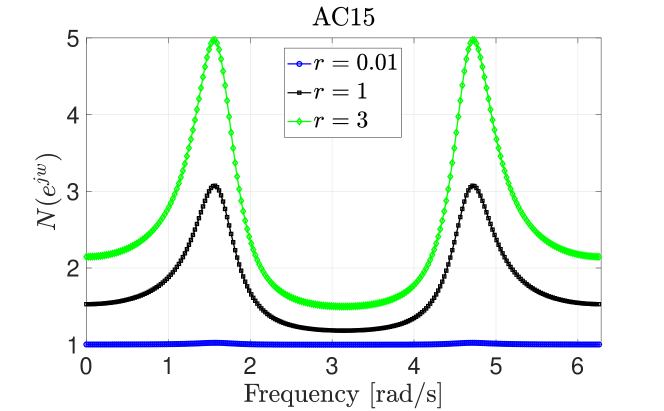
(a) The frequency domain representation of $\mathcal{N}$ for $r=0.01,1,3$ for system [AC15].

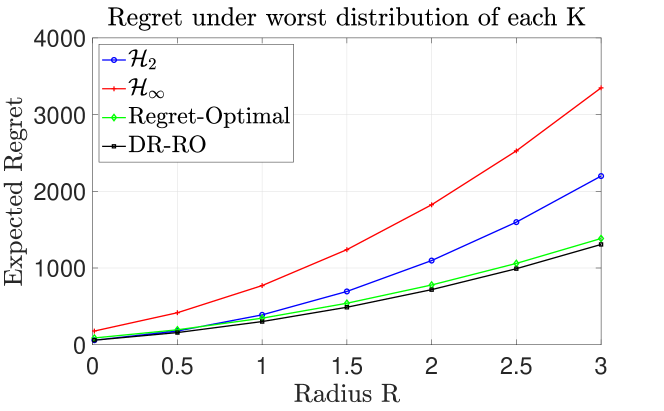
(b) The worst-case expected regret of different controllers for the system [AC15].

Figure 1: Variation of $\mathcal{N}$ with $r$ and the performance of the DR-RO controller versus the $\mathit{H}_{2},\mathit{H}_{\infty}$, and $RO$ controller.

While the objective function in Equation 26 is convex with respect to $\mathcal{P}$ and $\mathcal{Q}$ individually, it is not jointly convex in $(\mathcal{P},\mathcal{Q})$. In this form, 5.2 is not amenable to standard convex optimization tools.

To circumvent this issue, we instead consider the sublevel sets of the objective function in Equation 26.

Definition 5.3.

For a given $\epsilon>0$ approximation bound, the $\epsilon$-sublevel set of 5.2 is defined as

$$\vspace{-3mm}\mathscr{S}_{\epsilon}\!\coloneqq\!\left\{{(\mathcal{P},\mathcal{Q})\,\left|\;\left\|{{\mathcal{P}/\mathcal{Q}}\!-\!\mathcal{N}}\right\|_{\infty}\!\!\leq\!\epsilon,\;\operatorname{tr}(\mathcal{Q})\!=\!1\right.}\right\}.$$

By applying the definition of $\mathit{H}_{\infty}$-norm, we have that

$$\left\|{{\mathcal{P}/\mathcal{Q}}\!-\!\mathcal{N}}\right\|_{\infty}\!\!\!=\!\max_{z\in\mathbb{T}}\left|{{P(z)/Q(z)}-{N(z)}}\right|\leq\epsilon$$

$$\iff\left\{\begin{aligned} &P(z)\!-\!\left({N(z)\!+\!\epsilon}\right){Q(z)}\!\leq\!0,\\ &{P(z)}\!-\!\left({N(z)\!-\!\epsilon}\right){Q(z)}\!\geq\!0,\end{aligned}\right.$$ (27)

where the last set of inequalities hold for all $z\in\mathbb{T}$. Notice that the inequalities in Equation 27 and the positivity constraints on $\mathcal{P},\mathcal{Q}$ are jointly affine in $(\mathcal{P},\mathcal{Q})$. Moreover, the equation $\operatorname{tr}(\mathcal{Q})=1$ is an affine equality constraint. Therefore, we have the following claim.

Lemma 5.4.

The set $\mathscr{S}_{\epsilon}$ is jointly convex in $(\mathcal{P},\mathcal{Q})$.

Unlike its non-convex optimization counterpart in 5.2, a membership oracle for the convex set $\mathscr{S}_{\epsilon}$ offers a means to obtain accurate rational approximations for non-rational functions. According to Lemma 5.1, the positive trig. polynomials $(\mathcal{P},\mathcal{Q})\in\mathscr{S}_{\epsilon}$ can be parameterized by psd matrices $\mathbf{P}$ and $\mathbf{Q}$. This allows the equality constraint $\operatorname{tr}(\mathcal{Q})$ and the affine inequalities in (27) to be expressed as Linear Matrix Inequalities (LMIs) in terms of $\mathbf{P}$ and $\mathbf{Q}$. The resulting theorem characterizes the $\epsilon$-sublevel sets.

Theorem 5.5 (Feasibility of $\mathscr{S}_{\epsilon}$).

Let $\epsilon\!>\!0$ be a given accuracy level, and $m\in\mathbb{N}$ is a fixed order. The trig. polynomials $\mathcal{P}$ and $\mathcal{Q}$ of order $m$ belong to the $\epsilon$-sublevel set, $(\mathcal{P},\mathcal{Q})\in\mathscr{S}_{\epsilon}$ if and only if there exists $\mathbf{P},\mathbf{Q}\in\mathbb{S}_{+}^{m+1}$ such that $\operatorname{tr}\left({\mathbf{Q}}\right)=1$ and for all $z\in\mathbb{T}$, .

$$\vspace{-3mm}1)\, \operatorname{tr}\left({\mathbf{P}\bm{\Theta}(z)}\right)\!-\!\left({N(z)\!+\!\epsilon}\right)\operatorname{tr}\left({\mathbf{Q}\bm{\Theta}(z)}\right)\!\leq\!0,$$ (28)

$$2)\, \operatorname{tr}\left({\mathbf{P}\bm{\Theta}(z)}\right)\!-\!\left({N(z)\!-\!\epsilon}\right)\operatorname{tr}\left({\mathbf{Q}\bm{\Theta}(z)}\right)\!\geq\!0.\vspace{-6mm}$$ (29)

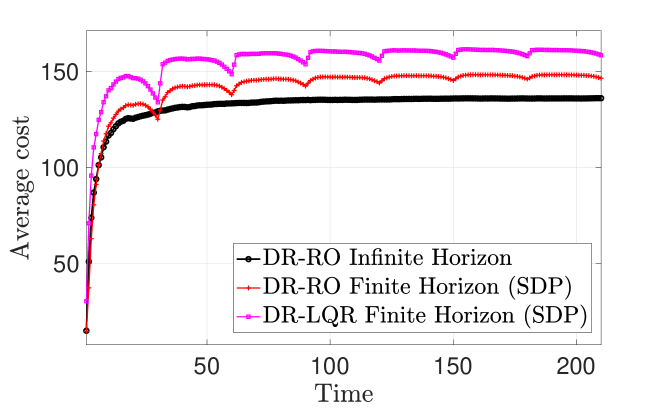
(a) White noise

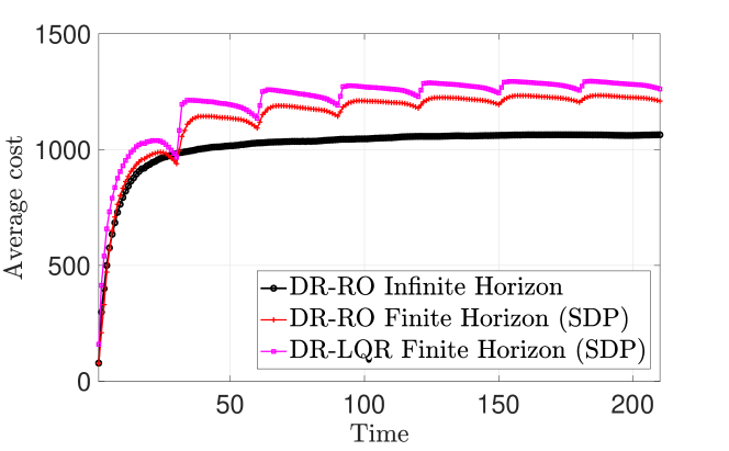
(b) Worst disturbance for DR-RO, infinite horizon

Figure 2: The control costs of different DR controllers under (a) white noise and (b) worst disturbance for DR-RO in infinite horizon, for system [AC15]. The finite-horizon controllers are re-applied every $s=30$ steps. The infinite horizon DR-RO controller achieves the lowest average cost compared to the finite-horizon controllers.

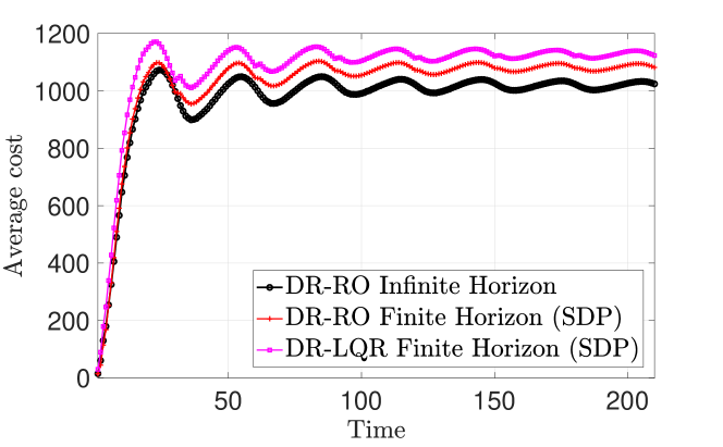
(a) Worst disturbance for DR-RO, finite horizon

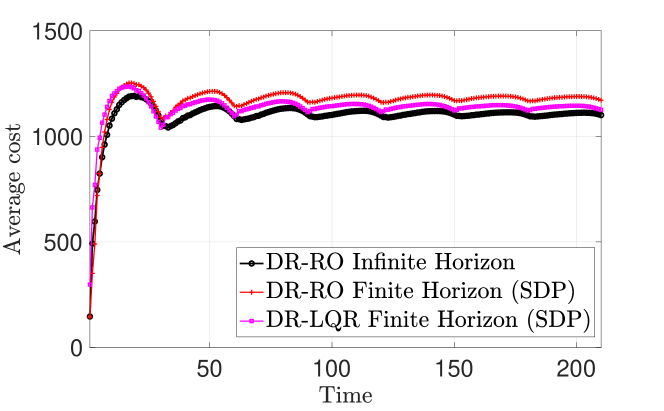
(b) Worst disturbance for DR-LQR, finite horizon

Figure 3: The control costs of different DR controllers under (a) worst disturbances for DR-RO in finite horizon and (b) worst disturbances for DR-LQR in finite horizon, for system [AC15]. The finite-horizon controllers are re-applied every $s=30$ steps. Despite being designed to minimize the cost under specific disturbances, the finite horizon DR controllers are outperformed by the infinite horizon DR-RO controller.

The sole limitation in this approach arises from the fact that for an non-rational $N(z)$, the set of infinitely many inequalities in (27) cannot be precisely characterized by a finite number of constraints, as seen in the trace parametrization of positive polynomials. To overcome this challenge, one can address the inequalities in (27) solely for a finite set of frequencies, such as $\mathbb{T}_{N}=\{\mathrm{e}^{j2\pi n/N}\mid n=0,\dots,N-1\}$ for $N\gg m$. While this introduces an approximation, the method’s accuracy can be enhanced arbitrarily by increasing the frequency samples. By taking this approach, the problem of rational function approximation can be reformulated as a convex feasibility problem involving LMIs and a finite number of affine (in)equality constraints.

It is crucial to note our algorithm can be used in the following two modes. These operational modes highlight the algorithm’s adaptability for the given two use cases.

1. Best Precision for a given degree By adjusting the parameter $\epsilon$, which signifies our tolerance for deviations from $M(e^{jw})$, we can refine the approximation’s accuracy. This method is particularly valuable when we need to find the best possible polynomial representation of $M(e^{jw})$ for a given degree.

2. Lowest Degree for a given precision In contrast, we can ask for the lowest degree polynomial which achieves a certain precision level $\epsilon$. This mode is advantageous when the priority is to minimize computational overhead or when we need a simpler polynomial approximation, as long as the approximation remains within acceptable accuracy bounds

5.3 Obtaining State-Space Controllers

Note that given the polynomial z-spectra, we require its spectral factorization to obtain the state-space controller that approximates the DR-RO controller. The following Lemma introduces a simple way to obtain such an approximation

Lemma 5.6 (Canonical factor of polynomial z-spectra (Sayed & Kailath, 2001, Lem. 1)).

Consider a Laurent polynomial of degree $m$, $P(z)=\sum_{k=-m}^{m}p_{k}z^{-k}$, with $p_{k}=p_{-k}\in\mathbb{R}$, such that $P(z)>0$. Then, there exists a canonical factor $L(z)=\sum_{k=0}^{m}\ell_{k}z^{-k}$ such that $P(z)=|{L(z)}|^{2}$ and $L(z)$ has all of its root in $\mathbb{T}$.

Using Lemma 5.6, we can compute spectral factors by factorizing the symmetric positive polynomials and multiplying all the factors with stable roots together. Consequently, this rational spectral factor enables the derivation of a rational controller, denoted as $K(z)$ (refer to Section 5.3).

Now we present the DR-RO controller in state-space form.

Lemma 5.7.

Let $\tilde{L}(z)$ be the rational factor of the spectral factorization $\tilde{N}(z)=\tilde{L}(z)^{\ast}\tilde{L}(z)\!=\!P(z)/Q(z)$ of a degree $m$ rational approximation $P(z)/Q(z)$. The controller obtained from $\tilde{L}(z)$ using (16), i.e., $K(z)\!=\!K_{\mathit{H}_{2}}(z)\!+\!\Delta(z)^{-1}\left\{{\{\Delta(z)K_{\circ}(z)\}_{-}\tilde{L}(z)}\right\}_{+}\tilde{L}(z)^{\mathrm{\!-\!1}}$ is rational and can be realized as a state-space controller as follows:

$$e(t+1)=\widetilde{F}e(t)+\widetilde{G}w(t),\quad u(t)=\widetilde{H}e(t)+\widetilde{J}w(t))\vspace{-2mm}$$ (30)

where $e_{t}$ is the controller state, and $(\widetilde{F},\widetilde{G},\widetilde{H},\widetilde{J})$ are determined from $(A,B_{u},B_{w})$ and $\tilde{L}(z)$.

6 Numerical Experiments

In this section, we present the performance of the DR-RO controller, compared to $H_{2}$, $H_{\infty}$, regret-optimal and other finite-horizon DR controllers. We present frequency domain and time-domain evaluations, and we showcase the performance of the rational approximation method. We employ benchmark models such as [REA4], [AC15], and [HE3] from (Leibfritz & Lipinski, 2003). In the frequency domain simulations, results for [REA4] and [HE3] are presented. In the time domain simulations for the aircraft model [AC15] are presented, with additional simulations provided in Appendix H. The [REA4] is a chemical reactor model and [HE3] is a helicopter model with 8 states each. The [AC15] is an aircraft model with 4 states. We perform all experiments using MATLAB, on an Apple M1 processor with 8 GB of RAM. We specify the nominal distribution as a Gaussian, with zero mean and identity covariance.

6.1 Frequency Domain Evaluations

We investigate the behaviour of the DR-RO controller and its rational approximation for various values of the radius $r$.

To show the behavior of the worst-case disturbance we plot its power spectrum $N(e^{j\omega})$ for three different values of the radius $r$ for the [AC15] system in Figure 1(a). As can be seen for $r=0.01$, the worst-case disturbance is almost white, since that is the case for the nominal disturbance. As $r$ increases, the time correlation of the worst-case disturbance increases, and the power spectrum becomes peaky.

For the [AC15] system, the worst-case expected regret cost, as outlined in (2.1), for DR-RO, the $\mathit{H}_{2}$, $\mathit{H}_{\infty}$, and RO controllers. are depicted in Figure 1(b). We observe that for smaller $r$, the DR-RO performs close to the $\mathit{H}_{2}$ controller. However, as $r$ increases, the worst-case regret is close to the regret achieved by the RO controller. Throughout the variation in $r$, the DR-RO achieves the lowest worst-case expected regret among all the other mentioned controllers.

To implement the DR-RO controller in practice, we need a rational controller. We find the rational approximation of $N(\mathrm{e}^{{j}\omega})$ as $\frac{P(\mathrm{e}^{{j}\omega})}{Q(\mathrm{e}^{{j}\omega})}$ using the method of Section 5.2 for [AC15] and degrees $m=1,2,3$. The performance of the resulting rational controllers is compared to the non-rational DR-RO in Table 1. As can be seen, the rational approximation with an order greater than 2 achieves an expected regret that well matches that of the non-rational for all values of $r$.

	r=0.01	r=1	r=1.5	r=2	r=3
$DRRO$	59.16	302.08	488.57	718.20	1307.12
RA(1)	60.49	33394.74	4475.70	9351.89	2376.77
RA(2)	59.58	303.33	491.75	723.96	1318.98
RA(3)	59.57	302.41	489.49	719.72	1309.85

Table 1: The worst-case expected regret of the non-rational DR-RO controller, compared to the rational controllers RA(1), RA(2), and RA(3), obtained from degree 1, 2, and 3 rational approximations to $N(e^{j\omega})$.

6.2 Time Domain Evaluations

We compare the time-domain performance of the infinite horizon DR-RO controller to its finite horizon counterparts, namely DR-RO and DR-LQR, as outlined in (Yan et al., 2023). The latter controllers are computed through an SDP whose dimension scales with the time horizon. We plot the average LQR cost over 210 time steps, aggregated over 1000 independent trials. Figure 2(a) illustrates the performance of DR controllers under white Gaussian noise, while 2(b), 3(a), and 3(b) demonstrate responses to worst-case noise scenarios dictated by each of the controllers, using $r=1.5$. For computational efficiency, the finite horizon controllers operate over a horizon of only $s=30$ steps and are re-applied every $s$ steps. Their worst-case disturbances in 3(a) and 3(b) are also generated every $s$ steps, resulting in correlated disturbances only within each $s$ steps. Our findings highlight the infinite horizon DR-RO controller’s superior performance over all four scenarios. Note that extending the horizon of the SDP for longer horizons to come closer to the infinite horizon performance is extremely computationally inefficient. These underscore the advantages of using the infnite horizon DR-RO controller.

7 Future Work

Our work presents a complete framework for solving the DR control problem in the full-information setting. Future generalizations would address our limitations. One is to extend the rational approximation method from single to multi input systems. Another is to extend the results to partially observable systems where the state is not directly accessible. Finally, it would be useful to incorporate adaptation as the controller learns disturbance statistics through observations.

Impact Statement

This paper presents work whose goal is to advance the field of Machine Learning. There are many potential societal consequences of our work, none which we feel must be specifically highlighted here.

Appendix

Appendix A Organization of the Appendix

This appendix is organized into several sections:

First, Appendix B provides notations, definitions, and remarks about the problem formulation and uniqueness of the spectral factorization.

Next, Appendix C contain proofs of the duality and optimality theorems in Section 3.

Subsequently, Appendix D is dedicated to proofs of lemmas and theorems related to the efficient algorithm discussed in Section 4, and Appendix E describes the pseudo-code of the algorithm.

Further, Appendix F contains the proof of the state-space representation of the controller presented in Section 5.

Finally, additional simulation results are presented in Appendix H.

Appendix B Notations, Definitions and Remarks

B.1 Notations

In the paper, we use the notations in Table 2 for brevity.

Symbol	Description
$x_{t}$	State at time $t$
$s_{t}$	Regulated output at time $t$
$u_{t}$	Control input at time $t$
$w_{t}$	Exogenous disturbance at time $t$
$A$	State transition matrix
$B_{u}$	Control input matrix
$B_{w}$	Disturbance input matrix
$C$	Regulated output matrix
$R$	Control input cost matrix
$\mathcal{F}_{T}$	Finite-horizon operator for control input
$\mathcal{G}_{T}$	Finite-horizon operator for disturbance
$\mathcal{F}$	Infinite-horizon operator for control input
$\mathcal{G}$	Infinite-horizon operator for disturbance
$\|\cdot\|$	Euclidean norm
$\|\cdot\|_{2}$	$\mathit{H}_{2}$ (Frobenius) norm
$\|\cdot\|_{\infty}$	$\textit{H}_{\infty}$ (operator) norm
$\mathbb{E}$	Expectation
$\mathscr{K}$	Set of causal (online) and time-invariant DFC policies
$\mathscr{K}_{T}$	Set of causal DFC policies over a horizon $T$
$\mathcal{R}_{\mathcal{K}}$	Regret operator
$\mathcal{M}$	Auto-covariance operator for disturbances
$\mathcal{L}$	Unique, causal and causally invertible spectral factor of $\mathcal{M}=\mathcal{L}\mathcal{L}^{\ast}$
$\mathcal{N}$	The unique positive definite operator equal to $\mathcal{L}^{\ast}\mathcal{L}$
$\mathsf{W_{2}}$	Wasserstein-2 metric
$\mathcal{S}$	Symmetric positive polynomial matrix
$\text{tr}(\cdot)$	Trace of a Toeplitz operator
$\{\cdot\}_{+}$	Causal part of an operator
$\{\cdot\}_{-}$	Strictly anti-causal part of an operator
$\sqrt{\mathcal{M}},\textrm{ or }\mathcal{M}^{\frac{1}{2}}$	Symmetric positive square root of an operator or matrix
$\mathbb{S}_{n}^{+}$	The set of positive semidefinite matrices
$\mathscr{T}_{m,+}$	The set of positive trigonometric polynomials of degree $m$

Table 2: Notation Table

B.2 Explicit Form of Finite-Horizon State Space Model

Consider the restrictions of the infinite-horizon dynamics in (3) to the finite horizon as

$$\mathbf{s}_{T}=\mathcal{F}_{T}\mathbf{u}_{T}+\mathcal{G}_{T}\mathbf{w}_{T}.$$ (31)

The causal linear measurement model for the finite-horizon case in (31) can be stated explicitly as follows:

$$\underbrace{\begin{bmatrix}s_{0}\\ s_{1}\\ s_{2}\\ \vdots\\ s_{T}\end{bmatrix}}_{\mathbf{s}_{T}}=\underbrace{\begin{bmatrix}0&0&0&\dots&0\\ B_{u}&0&0&\dots&0\\ AB_{u}&B_{u}&0&\dots&0\\ \vdots&\vdots&\vdots&\ddots&\vdots\\ A^{T-1}B_{u}&A^{T-2}B_{u}&A^{T-3}B_{u}&\ddots&0\end{bmatrix}}_{\mathcal{F}_{T}}\underbrace{\begin{bmatrix}u_{0}\\ u_{1}\\ u_{2}\\ \vdots\\ u_{T}\end{bmatrix}}_{\mathbf{u}_{T}}+\underbrace{\begin{bmatrix}0&0&0&\dots&0\\ B_{w}&0&0&\dots&0\\ AB_{w}&B_{w}&0&\dots&0\\ \vdots&\vdots&\vdots&\ddots&\vdots\\ A^{T-1}B_{w}&A^{T-2}B_{w}&A^{T-3}B_{w}&\ddots&0\end{bmatrix}}_{\mathcal{G}_{T}}\underbrace{\begin{bmatrix}w_{0}\\ w_{1}\\ w_{2}\\ \vdots\\ w_{T}\end{bmatrix}}_{\mathbf{w}_{T}}$$ (32)

B.3 A Note about Robustness to Disturbances vs Robustness to Model Uncertainties

In our approach, we consider distributional robustness against disturbances, which provides flexibility, adaptability, and dynamic responses to unforeseen events. Although we do not explicitly address model uncertainties, these uncertainties can be effectively lumped together as disturbances—a technique known as uncertainty/disturbance lumping. This approach is particularly effective when the model uncertainties are relatively small. By treating parameter uncertainties as disturbances, we simplify system analysis and ensure that the controller is robust not only to known uncertainties but also to unexpected variations and modeling errors.

B.4 A note about the Uniqueness of the spectral factor $\mathcal{L}$

In Theorem 3.2, given that $\mathcal{L}$ is the causal and causally invertible spectral factor of $\mathcal{M}=\mathcal{L}\mathcal{L}^{\ast}$, it is unique up to a unitary transformation of its block-elements from the right. Fixing the choice of the unitary transformation in the spectral factorization (eg. positive-definite factors at infinity (Ephremidze et al., 2018)) results in a unique $\mathcal{L}$.

Appendix C Proof of Optimality Theorems

C.1 Proof of Theorem 3.1

This result is proven in detail in Kargin et al. (2023, Appendix A1). Due to its length, we provide only a brief sketch here. Interested readers can refer to Kargin et al. (2023) for the complete proof.For completeness, we provide the following proof sketch.

First, we provide a finite-horizon counterpart of the strong duality result from (Taha et al., 2023). Then, we reformulate the objective functions of both the finite-horizon and infinite-horizon dual problems using normalized spectral measures. We demonstrate the pointwise convergence of the finite-horizon dual objective function to the infinite-horizon objective by analyzing the limiting behavior of the spectrum of Toeplitz matrices. Finally, we show that the infinite-horizon dual problem attains a finite value and that the limits of the optimal values (and solutions) of the finite-horizon dual problem coincide with those of the infinite-horizon dual problem.

C.2 Proof of Theorem 3.2

The proof involves four main steps.

• Reformulation using Lemma C.1: Using Lemma C.1, we reformulate the original optimization problem. This lemma allows the expression of the convex mapping $\mathcal{X}\mapsto\operatorname{tr}(\mathcal{X}^{-1})$ using Fenchel duality, which transforms the objective function into a form that involves the supremum over a positive semi-definite matrix $\mathcal{M}$ and the only term depending on $\mathcal{K}$ remains $\operatorname{tr}(\mathcal{R}_{\mathcal{K}}\mathcal{M})$.

• Application of Wiener-Hopf Technique: We then Lemma C.2, which provides a method to approximate a non-causal controller by a causal one, minimizing the cost $\operatorname{tr}(\mathcal{R}_{\mathcal{K}}\mathcal{M})$. The optimal causal controller $\mathcal{K}_{\star}$ is derived using the Weiner-Hopf Technique.

• Karush-Kuhn-Tucker (KKT) Conditions: We then find the conditions on the optimal $\mathcal{M}$. This involves simplifying the objective function and finding the optimal $\mathcal{M}_{\gamma}$ and $\mathcal{K}_{\gamma}$ for the level $\gamma$.

• Final Reformulation and Duality: We further simplify the problem and apply strong duality to achieve the final form. The optimal $\mathcal{K}_{\star}$ is then derived from the Wiener-Hopf technique, with $\gamma_{\star}$ and $\mathcal{M}_{\star}$ obtained through duality arguments.

Before proceeding with the proof, we first state two useful lemmas

Lemma C.1.

The convex mapping $\mathcal{X}\!\mapsto\!\operatorname{tr}\mathcal{X}^{\mathrm{\!-\!1}}$ for $\mathcal{X}\!\succ\!0$ can be expressed via Fenchel duality as

$$\sup_{\mathcal{M}\succ 0}-\operatorname{tr}(\mathcal{X}\mathcal{M})+2\operatorname{tr}(\sqrt{\mathcal{M}})=\begin{cases}\operatorname{tr}(\mathcal{X}^{-1}),&\quad\text{if }\mathcal{X}\succ 0\\ +\infty,&\quad\text{o.w.}\end{cases}$$ (33)

Proof.

Observe that the objective $-\operatorname{tr}(\mathcal{X}\mathcal{M})+2\operatorname{tr}(\sqrt{\mathcal{M}})$ is concave in $\mathcal{M}$, and the expression on the right-hand side can be obtained by solving for $\mathcal{M}$. When $\mathcal{X}\not\succeq 0$, i.e., $\mathcal{X}$ may have negative eigenvalues, then the expression $\operatorname{tr}(\mathcal{X}\mathcal{M})$ can be made arbitrarily negative, and $\operatorname{tr}(\sqrt{\mathcal{M}})$ arbitrarily large, by chosing an appropriate $\mathcal{M}$. ∎

The following lemma will be useful in the proof of Theorem 3.2.

Lemma C.2 (Wiener-Hopf Technique (Kailath et al., 2000)).

Consider the problem of approximating a non causal controller $\mathcal{K}_{\circ}$ by a causal controller $\mathcal{K}$, such that $\mathcal{K}$ minimises the cost $\operatorname{tr}(\mathcal{R}_{\mathcal{K}}\mathcal{M})$, i.e.,

$$\inf_{\mathcal{K}\in\mathscr{K}}\operatorname{tr}(\mathcal{R}_{\mathcal{K}}\mathcal{M})$$ (34)

where $\mathcal{M}\succ 0$, $\mathcal{R}_{\mathcal{K}}=\left(\mathcal{K}-\mathcal{K}_{\circ}\right)^{\ast}\Delta^{\ast}\Delta\left(\mathcal{K}-\mathcal{K}_{\circ}\right)$ and $\mathcal{K}_{\circ}$ is the non-causal controller that makes the objective defined above zero. Then, the solution to this problem is given by

$$\mathcal{K}_{\star}=\Delta^{\mathrm{\!-\!1}}\left\{{\Delta\mathcal{K}_{\circ}\mathcal{L}}\right\}_{\!+}\mathcal{L}^{\mathrm{\!-\!1}},$$ (35)

where $\mathcal{L}$ is the unique causal and causally invertible spectral factor of $\mathcal{M}$ such that $\mathcal{M}=\mathcal{L}\mathcal{L}^{\ast}$ and $\left\{{\cdot}\right\}_{\!+}$ denotes the causal part of an operator. Alternatively, the controller can be written as,

$$\mathcal{K}_{\star}=\mathcal{K}_{\mathit{H}_{2}}+\Delta^{-1}\left\{{\{\Delta\mathcal{K}_{\circ}\}_{-}\mathcal{L}_{\star}}\right\}_{+},$$ (36)

where $\mathcal{K}_{\mathit{H}_{2}}\!\coloneqq\!\Delta^{\mathrm{\!-\!1}}\{\Delta\mathcal{K}_{\circ}\}_{\!+}$.

Proof.

Let $\mathcal{L}$ be the unique causal and causally invertible spectral factor of $\mathcal{M}$, i.e. $\mathcal{M}=\mathcal{L}\mathcal{L}^{\ast}$. Then, using the cyclic property of $\operatorname{tr}$, the objective can be written as,

$$\inf_{\mathcal{K}\in\mathscr{K}}\operatorname{tr}(\Delta\left(\mathcal{K}-\mathcal{K}_{\circ}\right)\mathcal{M}\left(\mathcal{K}-\mathcal{K}_{\circ}\right)^{\ast}\Delta^{\ast}) =\inf_{\mathcal{K}\in\mathscr{K}}\operatorname{tr}(\left(\Delta\mathcal{K}-\Delta\mathcal{K}_{\circ}\right)\mathcal{L}\mathcal{L}^{\ast}\left(\Delta\mathcal{K}-\Delta\mathcal{K}_{\circ}\right)^{\ast})$$ (37)

$$=\inf_{\mathcal{K}\in\mathscr{K}}\operatorname{tr}(\left(\Delta\mathcal{K}\mathcal{L}-\Delta\mathcal{K}_{\circ}\mathcal{L}\right)\left(\Delta\mathcal{K}\mathcal{L}-\Delta\mathcal{K}_{\circ}\mathcal{L}\right)^{\ast})$$ (38)

$$=\inf_{\mathcal{K}\in\mathscr{K}}\left\|\Delta\mathcal{K}\mathcal{L}-\Delta\mathcal{K}_{\circ}\mathcal{L}\right\|^{2}_{2}.$$ (39)

Since $\Delta,\mathcal{K}$ and $\mathcal{L}$ are causal, and $\Delta\mathcal{K}_{\circ}\mathcal{L}$ can be broken into causal and non-causal parts, it is evident that the controller that minimizes the objective is the one that makes the term $\Delta\mathcal{K}\mathcal{L}-\Delta\mathcal{K}_{\circ}\mathcal{L}$ strictly anti-causal, cancelling off the causal part of $\Delta\mathcal{K}_{\circ}\mathcal{L}$. This means that the optimal controller satisfies,

$$\Delta\mathcal{K}_{\star}\mathcal{L}=\left\{{\Delta\mathcal{K}_{\circ}\mathcal{L}}\right\}_{\!+}.$$ (40)

Also, since $\mathcal{L}^{\mathrm{\!-\!1}}$ and $\Delta^{\mathrm{\!-\!1}}$ are causal, the optimal causal controller is given by (35). Finally, using the fact that $\Delta\mathcal{K}_{\circ}=\left\{{\Delta\mathcal{K}_{\circ}}\right\}_{\!+}+\left\{{\Delta\mathcal{K}_{\circ}}\right\}_{\!-}$ and simplifying, we get (36). ∎

Proof of Theorem 3.2.

We first simplify our optimization problem (13) using Lemma C.1. We then find the conditions on the optimal optimization variables using Karush-Kuhn-Tucker (KKT) conditions. Using Lemma C.1, we can write,

$$\inf_{\begin{subarray}{c}\mathcal{K}\in\mathscr{K},\\ \gamma\mathcal{I}\succ\mathcal{R}_{\mathcal{K}}\end{subarray}}\operatorname{tr}((\mathcal{I}-\gamma^{\mathrm{\!-\!1}}\mathcal{R}_{\mathcal{K}})^{\!-\!1}\mathcal{M}_{\circ}) =\inf_{\mathcal{K}\in\mathscr{K}}\sup_{\mathcal{M}\succ 0}-\operatorname{tr}((\mathcal{I}-\gamma^{\mathrm{\!-\!1}}\mathcal{R}_{\mathcal{K}})\mathcal{M})+2\operatorname{tr}\left(\sqrt{\mathcal{M}^{\frac{1}{2}}_{\circ}\mathcal{M}\mathcal{M}^{\frac{1}{2}}_{\circ}}\right)$$

$$=\sup_{\mathcal{M}\succ 0}-\operatorname{tr}(\mathcal{M})+2\operatorname{tr}\left(\sqrt{\mathcal{M}^{\frac{1}{2}}_{\circ}\mathcal{M}\mathcal{M}^{\frac{1}{2}}_{\circ}}\right)+\inf_{\mathcal{K}\in\mathscr{K}}\gamma^{\mathrm{\!-\!1}}\operatorname{tr}(\mathcal{R}_{\mathcal{K}}\mathcal{M})$$

Fixing $\gamma\geq 0$, we focus on the reduced subproblem of (14),

$$\sup_{\mathcal{M}\succ 0}-\gamma\operatorname{tr}(\mathcal{M})-\gamma\operatorname{tr}(\mathcal{M}_{\circ})+2\gamma\operatorname{tr}\left(\sqrt{\mathcal{M}^{\frac{1}{2}}_{\circ}\mathcal{M}\mathcal{M}^{\frac{1}{2}}_{\circ}}\right)+\inf_{\mathcal{K}\in\mathscr{K}}\operatorname{tr}(\mathcal{R}_{\mathcal{K}}\mathcal{M}).$$ (41)

Using the definition of the Bures-Wasserstein distance, we can reformulate (41) as

$$\sup_{\mathcal{M}\succ 0}\inf_{\mathcal{K}\in\mathscr{K}}\operatorname{tr}(\mathcal{R}_{\mathcal{K}}\mathcal{M})\!-\!\gamma\operatorname{\mathsf{BW}}(\mathcal{M},\mathcal{M}_{\circ})^{2}\coloneqq\sup_{\mathcal{M}\succ 0}\Phi(\mathcal{M}).$$ (42)

Thus, the original formulation in (14) can be expressed as

$$\inf_{\gamma\geq 0}\sup_{\mathcal{M}\succ 0}\inf_{\mathcal{K}\in\mathscr{K}}\operatorname{tr}(\mathcal{R}_{\mathcal{K}}\mathcal{M})+\gamma\left({r^{2}-\operatorname{\mathsf{BW}}(\mathcal{M},\mathcal{M}_{\circ})^{2}}\right).$$ (43)

Note that the objective above is affine in $\gamma\geq 0$ and strictly concave in $\mathcal{M}$. Moreover, primal and dual feasibility hold, enabling the exchange of $\inf_{\gamma\geq 0}\sup_{\mathcal{M}\succ 0}$ resulting in

$$\sup_{\mathcal{M}\succ 0}\inf_{\mathcal{K}\in\mathscr{K}}\inf_{\gamma\geq 0}\operatorname{tr}(\mathcal{R}_{\mathcal{K}}\mathcal{M})+\gamma\left({r^{2}-\operatorname{\mathsf{BW}}(\mathcal{M},\mathcal{M}_{\circ})^{2}}\right),$$ (44)

where the inner minimization over $\gamma$ reduces the problem to its constrained version in Equation 15.

Finally, the form of the optimal $\mathcal{K}_{\star}$ follows from the Wiener-Hopf technique in Lemma C.2 and the optimal $\gamma_{\star}$ and $\mathcal{M}_{\star}$ can be obtained using the strong duality result in Section C.1. To see the optimal form of $\mathcal{M}_{\star}$, consider the gradient of $\Phi(\mathcal{M})$ in (42) with respect to $\mathcal{M}$ and setting it to $0$. Using Danskin theorem (Danskin, 1966), we have,

$$\nabla\Phi(\mathcal{M})=\mathcal{M}^{\frac{1}{2}}_{\circ}\left(\mathcal{M}_{\circ}^{\frac{1}{2}}\mathcal{M}_{\star}\mathcal{M}_{\circ}^{\frac{1}{2}}\right)^{-\frac{1}{2}}\mathcal{M}^{\frac{1}{2}}_{\circ}-\mathcal{I}+\gamma^{-1}\mathcal{R}_{\mathcal{K}_{\star}}=0.$$ (45)

Taking inverse on both sides, we get,

$$\mathcal{M}^{-\frac{1}{2}}_{\circ}\left(\mathcal{M}_{\circ}^{\frac{1}{2}}\mathcal{M}_{\star}\mathcal{M}_{\circ}^{\frac{1}{2}}\right)^{\frac{1}{2}}\mathcal{M}^{-\frac{1}{2}}_{\circ}=\left(\mathcal{I}-\gamma^{-1}\mathcal{R}_{\mathcal{K}_{\star}}\right)^{-1}.$$ (46)

We can now obtain two equations. First, by right multiplying by $\mathcal{M}^{\frac{1}{2}}_{\circ}$ and second, by left multiplying by $\mathcal{M}^{\frac{1}{2}}_{\circ}$. On multiplying these two equations together and simplifying, we get (16b).

Appendix D Proofs related to the Efficient Algorithm in Section 4

D.1 Proof of Lemma 4.1

With $\mathcal{T}\coloneqq\{\Delta\mathcal{K}_{\circ}\}_{-}$, the optimality condition in (16) takes the equivalent form:

$$\textit{i.}\;\mathcal{M}_{\star}=\left({\mathcal{I}-\gamma_{\star}^{\mathrm{\!-\!1}}\mathcal{R}_{\mathcal{K}_{\star}}}\right)^{-2},$$ (47a)

$$\textit{ii.}\;\mathcal{R}_{\mathcal{K}_{\star}}\!=\!\mathcal{L}_{\star}^{\!-\!\ast}\left\{{\mathcal{T}\mathcal{L}_{\star}}\right\}_{\!-\!}^{\ast}\left\{{\mathcal{T}\mathcal{L}_{\star}}\right\}_{\!-\!}\mathcal{L}_{\star}^{\!-\!1},$$ (47b)

$$\textit{iii.}\;\operatorname{tr}\left[{\left({(\mathcal{I}-\gamma_{\star}^{\mathrm{\!-\!1}}\mathcal{R}_{\mathcal{K}_{\star}}(z))^{\mathrm{\!-\!1}}-\mathcal{I}}\right)^{2}}\right]=r^{2},$$ (47c)

Using the spectral factorization $\mathcal{M}_{\star}\mathcal{L}_{\star}\mathcal{L}_{\star}^{\ast}$, the conditions i. and ii. can be equivalently re-expressed as

$$\textit{i.}\;(\mathcal{L}_{\star}\mathcal{L}_{\star}^{\ast})^{-1/2}=I-\gamma_{\star}^{\mathrm{\!-\!1}}\mathcal{R}_{\mathcal{K}_{\star}}$$ (48)

$$\textit{ii.}\;\mathcal{R}_{\mathcal{K}_{\star}}\!=\!\mathcal{L}_{\star}^{\!-\!\ast}\left\{{\mathcal{T}\mathcal{L}_{\star}}\right\}_{\!-\!}^{\ast}\left\{{\mathcal{T}\mathcal{L}_{\star}}\right\}_{\!-\!}\mathcal{L}_{\star}^{\!-\!1}$$ (49)

By plugging ii. into i., we get

$$0=\mathcal{I}-(\mathcal{L}_{\star}\mathcal{L}_{\star}^{\ast})^{-1/2}-\gamma_{\star}^{\mathrm{\!-\!1}}\left({\mathcal{L}_{\star}^{\!-\!\ast}\left\{{\mathcal{T}\mathcal{L}_{\star}}\right\}_{\!-\!}^{\ast}\left\{{\mathcal{T}\mathcal{L}_{\star}}\right\}_{\!-\!}\mathcal{L}_{\star}^{\!-\!1}}\right)=0,$$ (50)

Multiplying by $\mathcal{L}_{\star}^{\ast}$ from the left and by $\mathcal{L}_{\star}$ from the right, we get

$$0 =\mathcal{L}_{\star}^{\ast}\mathcal{L}_{\star}\!-\!(\mathcal{L}_{\star}^{\ast}\mathcal{L}_{\star})^{1/2}\!-\!\gamma_{\star}^{\mathrm{\!-\!1}}\left\{{\mathcal{T}\mathcal{L}_{\star}}\right\}_{\!-\!}^{\ast}\left\{{\mathcal{T}\mathcal{L}_{\star}}\right\}_{\!-\!},$$

where we used the identity $\mathcal{L}_{\star}^{\ast}(\mathcal{L}_{\star}\mathcal{L}_{\star}^{\ast})^{-1/2}\mathcal{L}_{\star}=(\mathcal{L}_{\star}^{\ast}\mathcal{L}_{\star})^{1/2}$. Letting $\mathcal{N}_{\star}=\mathcal{L}_{\star}^{\ast}\mathcal{L}_{\star}$, this expression can be solved for $\mathbb{N}_{\star}$, yielding the following implicit equation,

$$\mathcal{N}_{\star}=\mathcal{L}_{\star}^{\ast}\mathcal{L}_{\star}=\frac{1}{4}\left({\mathcal{I}+\sqrt{\mathcal{I}+4\gamma_{\star}^{\mathrm{\!-\!1}}\left\{{\mathcal{T}\mathcal{L}_{\star}}\right\}_{\!-\!}^{\ast}\left\{{\mathcal{T}\mathcal{L}_{\star}}\right\}_{\!-\!}}}\right)^{2},$$ (51)

implying thus (17), with $\gamma_{\star}\!>\!0$ satisfying $\operatorname{tr}\left[{((\mathcal{I}-\gamma_{\star}^{\mathrm{\!-\!1}}\mathcal{R}_{\mathcal{K}_{\star}})^{\mathrm{\!-\!1}}-\mathcal{I})^{2}}\right]=r^{2}$ (or equivalently, $\operatorname{\mathsf{BW}}(\mathcal{L}_{\star}\mathcal{L}_{\star}^{\ast},\mathcal{I})=r$).∎

D.2 Note on Frequency Domain Representation of Toeplitz Operators

We start this section of the appendix by justifying our choice of working out our results in the frequency domain.

Let $\mathcal{V}=[V_{ij}]_{i,j=-\infty}^{\infty}$ be a doubly infinite block matrix, i.e.a Toeplitz operator, which represents a discrete, linear, time-invariant system (i.e.$V_{ij}=V_{i-j}$), and which maps a sequence of inputs to a sequence of outputs.

In this case of a time-invariant system, the representation of the operator in the z-domain (or the so-called bilateral z-transform) is

$$V(z)=\sum_{i=-\infty}^{\infty}V_{i}z^{-i},$$ (52)

defined for the regions of the complex plane where the above series converges absolutely, known as the ROC: region of convergence. $V(z)$ is also known as the transfer matrix. The causality of $\mathcal{V}$ can be readily given in terms of $V(z)$. Indeed, we have the following: $\mathcal{V}$ is causal if and only if $V(z)$ is analytic in the exterior of some annulus, $|z|>\alpha>0$. Likewise, $\mathcal{V}$ is anticausal if and only if $V(z)$ is analytic in the interior of some annulus, $|z|<\alpha<0$. Moreover, $\mathcal{V}$ is strictly causal (anticausal) if and only if it is causal (anticausal) and $V(\infty)=0(V(0)=0)$.

We also define the trace of a Toeplitz operator $\mathcal{M}$ as follows

$$\operatorname{tr}(\mathcal{M})=\frac{1}{2\pi}\int_{0}^{2\pi}\operatorname{Tr}(M(\mathrm{e}^{{j}\omega}))d\omega.$$ (53)

In the coming sections, we use the frequency domain counterparts of our Toeplitz operators (such as $\mathcal{F},\mathcal{G},\mathcal{M}...$) by setting $z=e^{j\omega}$ for $\omega\in[0,2\pi)$.

D.3 Frequency-Domain Characterization of the Optimal Solution of 2.3

We present the frequency-domain formulation of the saddle point $(\mathcal{K}_{\star},\mathcal{M}_{\star})$ derived in Theorem 3.2 to reveal the structure of the solution. We first introduce the following useful results:

Denoting by $M_{\star}(z)$ and $R_{K_{\star}}(z)$ the transfer functions corresponding to the optimal $\mathcal{M}_{\star}$ and $\mathcal{R}_{\mathcal{K}_{\star}}$, respectively, the optimality conditions in (16) and (17) take the equivalent forms:

$$\textit{i.}\;M_{\star}(z)=\left({I-\gamma_{\star}^{\mathrm{\!-\!1}}R_{K_{\star}}(z)}\right)^{-2},$$ (54a)

$$\textit{ii.}\;R_{K_{\star}}(z)\!=\!L_{\star}(z)^{\!-\!\ast}\left\{{\mathcal{T}\mathcal{L}_{\star}}\right\}_{\!-\!}(z)^{\ast}\left\{{\mathcal{T}\mathcal{L}_{\star}}\right\}_{\!-\!}(z)L_{\star}(z)^{\!-\!1},$$ (54b)

$$\textit{iii.}\;\operatorname{tr}\left[{\left({(I-\gamma_{\star}^{\mathrm{\!-\!1}}R_{K_{\star}}(z))^{\mathrm{\!-\!1}}-I}\right)^{2}}\right]=r^{2},,$$ (54c)

$$\textit{iv.}\;N_{\star}(z)=L_{\star}(z)^{\ast}L_{\star}(z)=\frac{1}{4}\left({I+\sqrt{I+4\gamma^{\mathrm{\!-\!1}}\left\{{\mathcal{T}\mathcal{L}_{\star}}\right\}_{\!-\!}(z)^{\ast}\left\{{\mathcal{T}\mathcal{L}_{\star}}\right\}_{\!-\!}(z)}}\right)^{2},$$ (54d)

where

$$L_{\star}(z)=\sum_{t=0}^{\infty}\widehat{L}_{\star,t}z^{-t}$$ (55)

is the transfer function corresponding to the causal canonical factor $\mathcal{L}_{\star}$ and $\mathcal{T}=\{\Delta\mathcal{K}_{\circ}\}_{-}$ is the strictly anticausal operator where its transfer function, $T(z)$, is found from the following:

Lemma D.1 (Adapted from lemma 4 in (Sabag et al., 2021)).

The transfer function $\Delta(z)K_{\circ}(z)$ can be written as the sum of a causal and strictly anticausal transfer functions:

$$\Delta(z)K_{\circ}(z)=T(z)+U(z)$$ (56)

$$T(z)=\{\Delta\mathcal{K}_{\circ}\}_{\!-\!}(z)=\overline{C}{(z^{-1}I-\overline{A})}^{-1}\overline{B}$$ (57)

$$U(z)=\{\Delta\mathcal{K}_{\circ}\}_{\!+\!}(z)=\Delta(z)K_{H_{2}}(z)=\overline{C}P(A{(zI-A)}^{-1}+I)B_{w}$$ (58)

where $K_{H_{2}}(z)=\Delta^{\!-\!1}\{\Delta\mathcal{K}_{\circ}\}_{\!+\!}(z)$, and $K_{\textrm{lqr}}\!\coloneqq\!{(I\!+\!B_{u}^{\ast}PB_{u})}^{\mathrm{\!-\!1}}B^{\ast}_{u}PA$, with $P\!\succ\!0$ is the unique stabilizing solution to the LQR Riccati equation $P=Q+A^{\ast}PA-A^{\ast}PB_{u}{(I+B_{u}^{\ast}PB_{u})}^{-1}B_{u}^{\ast}PA,$ $Q=C^{\intercal}C,$ $A_{k}=A\!-\!B_{u}K_{\textrm{lqr}}$, and

$$\overline{A}=A_{k}^{\ast},\quad\overline{B}=A_{k}^{\ast}PB_{w},\quad\overline{C}=-(I+B_{u}^{\ast}PB_{u})^{-\ast/2}B_{u}^{\ast}.$$ (59)

Notice that given the causal $L(z)$ and strictly anti-causal $T(z)$, the strictly anti-causal part $\{T(z)L(z)\}_{-}$ has a state space representation, shown in the following lemma.

Lemma D.2.

Let $\mathcal{L}$ be a causal operator. The strictly anti-causal operator $\left\{{\mathcal{T}\mathcal{L}}\right\}_{\!-\!}$ possesses a state space representation as follows:

$$\left\{{\mathcal{T}\mathcal{L}}\right\}_{\!-\!}(z)=\overline{C}(z^{-1}I-\overline{A})^{-1}\Gamma,$$ (60)

where

$$\Gamma=\frac{1}{2\pi}\int_{0}^{2\pi}(I-\mathrm{e}^{{j}\omega}\overline{A})^{\mathrm{\!-\!1}}\overline{B}L(\mathrm{e}^{{j}\omega})d\omega.$$ (61)

Proof.

Let $L(z)=\sum_{t=0}^{\infty}\widehat{L}_{t}z^{-t}$ be the transfer function of $\mathcal{L}$. Using equations (56) and (57),(58), $S(z)\coloneqq\left\{{\Delta\mathcal{K}_{\circ}\mathcal{L}}\right\}_{\!-\!}(z)$, can be written as:

$$S(z) =\left\{{TL}\right\}_{\!-\!}(z)+\left\{{UL}\right\}_{\!-\!}(z)$$ (62)

$$\stackrel{{\scriptstyle(a)}}{{=}}\left\{{\overline{C}(zI-\overline{A})^{\mathrm{\!-\!1}}\overline{B}L(z)}\right\}_{\!-\!}$$ (63)

$$\stackrel{{\scriptstyle(b)}}{{=}}\left\{{\overline{C}\sum_{t=0}^{\infty}z^{(t+1)}\overline{A}^{t}\overline{B}\sum_{m=0}^{\infty}\widehat{L}_{m}z^{-m}}\right\}_{\!-\!}$$ (64)

$$\stackrel{{\scriptstyle(c)}}{{=}}{\overline{C}\left(\sum_{t=0}^{\infty}z^{(t+1)}\overline{A}^{t}\right)\left(\sum_{m=0}^{\infty}\overline{A}^{m}\overline{B}\widehat{L}_{m}\right)}$$ (65)

$$\stackrel{{\scriptstyle(d)}}{{=}}\overline{C}(z^{-1}I-\overline{A})^{-1}\Gamma$$ (66)

Here, (a) holds because both $U(z)$ and $L(z)$ are causal, so the strictly anticausal part of $U(z)L(z)$ is zero. (b) holds as we do the Neumann series expansion of $(zI-\overline{A})$ and replace $L(z)$ by its equation (55). (c) holds as we take the anticausal part of expression (64) to be the strictly positive exponents of $z$. (d) completes the result by using the Neuman series again, defining $\Gamma\coloneqq\sum_{t=0}^{\infty}\overline{A}^{t}\overline{B}\widehat{L}_{t}$, and leveraging Parseval’s theorem to conclude the equation of the finite parameter

$$\Gamma=\frac{1}{2\pi}\int_{0}^{2\pi}(I-\mathrm{e}^{{j}\omega}\overline{A})^{\mathrm{\!-\!1}}\overline{B}L(\mathrm{e}^{{j}\omega})d\omega.$$ (67)

∎

Proof of Theorem 4.2:

Using Lemma D.2, and plugging (60) into (54d), the frequency-domain optimality equation (54d) can be reformulated explicitly as follows

$$N_{\star}(z)=L_{\star}(z)^{\ast}L_{\star}(z)=\frac{1}{4}\left({I+\sqrt{I+4\gamma_{\star}^{\mathrm{\!-\!1}}\Gamma_{\star}^{\ast}(z^{-1}I-\overline{A})^{\!-\!\ast}\overline{C}^{\ast}\overline{C}(z^{\!-\!1}I-\overline{A})^{\!-\!1}\Gamma_{\star}}}\right)^{2}$$ (68)

where $\Gamma_{\star}$ as in (67), and $\gamma_{\star}\!>\!0$ satisfying $\operatorname{tr}\left[{((\mathcal{I}-\gamma_{\star}^{\mathrm{\!-\!1}}\mathcal{R}_{\mathcal{K}_{\star}})^{\mathrm{\!-\!1}}-\mathcal{I})^{2}}\right]=r^{2}$ (or equivalently, $\operatorname{\mathsf{BW}}(\mathcal{L}_{\star}\mathcal{L}_{\star}^{\ast},\mathcal{I})=r$), which gives the desired result. ∎

Proof of Corollary 4.3:

Notice that the rhs of (68) involves the positive definite square-root of the rational term $\Gamma_{\star}^{\ast}(z^{-1}I-\overline{A})^{\!-\!\ast}\overline{C}^{\ast}\overline{C}(z^{\!-\!1}I-\overline{A})^{\!-\!1}\Gamma_{\star}$. The square root does not preserve rationality in general, implying the desired result. ∎

D.4 Proof of Theorem 4.5

Before proceeding with the proof, we state the following useful lemma.

Lemma D.3.

For a positive-definite Toeplitz operator $\mathcal{M}\succ 0$ with $\operatorname{tr}(\mathcal{M})<\infty$ and $\operatorname{tr}(\log(\mathcal{M}))>-\infty$, let $\mathcal{M}\mapsto\Phi(\mathcal{M})$ be a mapping defined as

$$\Phi(\mathcal{M})\triangleq\inf_{\mathcal{K}\in\mathscr{K}}\operatorname{tr}\left({\mathcal{R}_{\mathcal{K}}\mathcal{M}}\right).$$ (69)

Denote by $\mathcal{M}=\mathcal{L}\mathcal{L}^{\ast}$ and $\Delta\Delta^{\ast}=\mathcal{I}+\mathcal{F}^{\ast}\mathcal{F}$ the canonical spectral factorizations where $\mathcal{L}$, $\Delta$ as well as their inverses $\mathcal{L}^{\mathrm{\!-\!1}}$, $\Delta^{\mathrm{\!-\!1}}$ are causal operators. The following statements hold:

• The function $\Phi$ can be written in closed form as

  $$\Phi(\mathcal{M})=\operatorname{tr}\left[{\left\{{\Delta\mathcal{K}_{\circ}\mathcal{L}}\right\}_{-}^{\ast}\left\{{\Delta\mathcal{K}_{\circ}\mathcal{L}}\right\}_{-}}\right].$$ (70)

• The gradient of $\Phi$ has the following closed form

  $$\nabla\Phi(\mathcal{M})=\mathcal{R}_{\mathcal{K}}=\mathcal{L}^{-\ast}\left\{{\Delta\mathcal{K}_{\circ}\mathcal{L}}\right\}_{-}^{\ast}\left\{{\Delta\mathcal{K}_{\circ}\mathcal{L}}\right\}_{-}\mathcal{L}^{-1}.$$ (71)

• The function $\Phi$ is concave, positively homogeneous, and

  $$\Phi(\mathcal{M})=\operatorname{tr}(\mathcal{M}\,\nabla\Phi(\mathcal{M})).$$ (72)

Proof of Theorem 4.5.

Our proof of convergence follows closely from the proof technique used in (Jaggi, 2013). In particular, since the unit circle is discretized and the computation of the gradients are approximate, the linear suboptimal problem is solved upto an approximation, $\delta_{N}$ which depends on the problem parameters and the discretization level $N$. Namely, for a large enough $N$, we have

$$\operatorname{tr}(\nabla\Phi(\mathcal{M}_{k})\widetilde{\mathcal{M}}_{k+1})\geq\sup_{\begin{subarray}{c}\mathcal{M}\in\Omega_{r}\end{subarray}}\operatorname{tr}(\nabla\Phi(\mathcal{M}_{k}){\mathcal{M}})-\delta_{N}$$ (73)

where

$$\Omega_{r}\coloneqq\{\mathcal{M}\succ 0\mid\operatorname{tr}(\mathcal{M}-2\sqrt{\mathcal{M}}+\mathcal{I})\leq r^{2}\},$$ (74)

Therefore, using Theorem 1 of (Jaggi, 2013), we obtain

$$\Phi(\mathcal{M}_{\star})-\Phi(\mathcal{M}_{k})\leq\frac{2\kappa}{k+2}(1+\delta_{N}).$$ (75)

where $\kappa>0$ is the so-called curvature constant associated with the problem which is defined as follows

$$\kappa \coloneqq\sup_{\begin{subarray}{c}\mathcal{M},\widetilde{\mathcal{M}}\in\Omega_{r}\\ \eta\in[0,1]\\ \mathcal{M}^{\prime}=\mathcal{M}+\eta(\widetilde{\mathcal{M}}-\mathcal{M})\end{subarray}}\frac{2}{\eta^{2}}\left[{-\Phi(\mathcal{M}^{\prime})+\Phi(\mathcal{M})+\operatorname{tr}(\nabla\Phi(\mathcal{M})\,(\mathcal{M}^{\prime}-\mathcal{M}))}\right],$$ (76)

$$=\sup_{\begin{subarray}{c}\mathcal{M},\widetilde{\mathcal{M}}\in\Omega_{r}\\ \eta\in[0,1]\\ \mathcal{M}^{\prime}=\mathcal{M}+\eta(\widetilde{\mathcal{M}}-\mathcal{M})\end{subarray}}\frac{2}{\eta^{2}}\left({\operatorname{tr}(\mathcal{M}^{\prime}\nabla\Phi(\mathcal{M}))-\Phi(\mathcal{M}^{\prime})}\right),$$ (77)

$$=\sup_{\begin{subarray}{c}\mathcal{M},\widetilde{\mathcal{M}}\in\Omega_{r}\\ \eta\in[0,1]\\ \mathcal{M}^{\prime}=\mathcal{M}+\eta(\widetilde{\mathcal{M}}-\mathcal{M})\end{subarray}}\inf_{\mathcal{K}\in\mathscr{K}}\frac{2}{\eta^{2}}\operatorname{tr}\left({\mathcal{M}^{\prime}(\nabla\Phi(\mathcal{M})-\mathcal{R}_{\mathcal{K}})}\right)$$ (78)

where the last two equalities follow from Lemma D.3.

Appendix E Algorithms

E.1 Pseudocode for Frequency-domain Iterative Optimization Method Solving (15)

The pseudocode for Frequency-domain tterative optimization method is presented in Algorithm 1.

Algorithm 1 Frequency-domain iterative optimization method solving (15)

1:  Input: Radius $r\!>\!0$, state-space model $(A,B_{u},B_{w})$, discretizations $N\!>\!0$ and $N^{\prime}\!>\!0$ tolerance $\epsilon\!>\!0$

2:  Compute $(\overline{A},\overline{B},\overline{C})$ from $(A,B_{u},B_{w})$ using (59)

3:  Generate frequency samples $\mathbb{T}_{N}\coloneqq\{\mathrm{e}^{j2\pi n/N}\mid n\!=\!0,\dots,N\!-\!1\}$

4:  Initialize $M_{0}(z)\leftarrow I$ for $z\in\mathbb{T}_{N}$, and $k\leftarrow 0$

5:  repeat

6:     Set the step size $\eta_{k}\leftarrow\frac{2}{k+2}$

7:     Compute the spectral factor $\begin{aligned} L_{k}(z)\leftarrow\texttt{SpectralFactor}(M_{k})\end{aligned}$ (see Algorithm 2)

8:     Compute the parameter $\begin{aligned} \Gamma_{k}\leftarrow\frac{1}{N}\sum\nolimits_{z\in\mathbb{T}_{N}}(I-z\overline{A})^{-1}\overline{B}L_{k}(z).\end{aligned}$ (see Section E.2)

9:     Compute the gradient for $z\in\mathbb{T}_{N}$ (see Section E.2) $\begin{aligned} \quad\quad R_{k}(z)\leftarrow L_{k}(z)^{-\ast}\left\{{\Delta\mathcal{K}_{\circ}\mathcal{L}_{k}}\right\}_{-}(z)^{\ast}\left\{{\Delta\mathcal{K}_{\circ}\mathcal{L}_{k}}\right\}_{-}(z)L_{k}(z)^{-1}\end{aligned}$

10:     Solve the linear subproblem (21a) via bisection (see Section E.4) $\begin{aligned} \quad\quad\widetilde{M}_{k}(z)\leftarrow(I-\gamma_{k}^{-1}R_{k}(z))^{-2}\end{aligned}$ for $z\in\mathbb{T}_{N}$ and $\gamma_{k}\text{ through }\texttt{Bisection}$

11:     Set $M_{k+1}(z)\leftarrow(1-\eta_{k})M_{k}(z)+\eta_{k}\widetilde{M}_{k}(z)$ for $z\in\mathbb{T}_{N}$.

12:     Increment $k\leftarrow k+1$

13:  until $\|{M_{k+1}-M_{k}}\|_{\text{}}/\|{M_{k}}\|_{\text{}}\leq\epsilon$

14:  Compute $N_{k}(z)=\frac{1}{4}\left({I+\sqrt{I+4\gamma_{k}^{-1}\Gamma_{k}^{\ast}(z^{-1}I-\overline{A})^{\!-\!\ast}\overline{C}^{\ast}\overline{C}(z^{-1}I-\overline{A})^{-1}\Gamma_{k}}}\right)^{2}$ for $z\in\mathbb{T}_{N^{\prime}}\coloneqq\{\mathrm{e}^{j2\pi n/N^{\prime}}\mid n\!=\!0,\dots,N^{\prime}\!-\!1\}$

15:  Compute $K(z)\leftarrow\texttt{RationalApproximate}(N_{k}(z))$ (see Section E.5)

E.2 Additional Discussion on the Computation of Gradients

By the Wiener-Hopf technique discussed in Lemma C.2, the gradient $\mathcal{R}_{k}=\nabla\Phi(\mathcal{M}_{k})$ can be obtained as

$$R_{k}(z)=L_{k}(z)^{-\ast}\left\{{\Delta\mathcal{K}_{\circ}\mathcal{L}_{k}}\right\}_{-}(z)^{\ast}\left\{{\Delta\mathcal{K}_{\circ}\mathcal{L}_{k}}\right\}_{-}(z)L_{k}(z)^{-1},$$ (79)

where $\mathcal{L}_{k}\mathcal{L}_{k}^{\ast}=\mathcal{M}_{k}$ is the unique spectral factorization. Furthermore, using (66),(67), we can reformulate the gradient $R_{k}(z)$ more explicitly as

$$R_{k}(z)=L_{k}(z)^{-\ast}\Gamma_{k}^{\ast}(I\!-\!z\overline{A})^{\!-\!\ast}\overline{C}^{\ast}\,\overline{C}(I\!-\!z\overline{A})^{\mathrm{\!-\!1}}\Gamma_{k}L_{k}(z)^{-1},$$ (80)

where $\Gamma_{k}=\frac{1}{2\pi}\int_{0}^{2\pi}(I-\mathrm{e}^{j\omega}\overline{A})^{\mathrm{\!-\!1}}\overline{B}L_{k}(\mathrm{e}^{j\omega})d\omega$ as in (67). Here, the spectral factor $L_{k}(z)$ is obtained for $z\in\mathbb{T}_{N}$ by Algorithm 2. Similarly, the parameter $\Gamma_{k}$ can be computed numerically using trapezoid rule over the discrete domain $\mathbb{T}_{N}$, i.e.,

$$\Gamma_{k}\leftarrow\frac{1}{N}\sum_{z\in\mathbb{T}_{N}}(I-z\overline{A})^{\mathrm{\!-\!1}}\overline{B}L_{k}(z).$$ (81)

The gradient $R_{k}(z)$ can thus be efficiently computed for $z\in\mathbb{T}_{N}$.

E.3 Implementation of Spectral Factorization

To perform the spectral factorization of an irrational function $M(z)$, we use a spectral factorization method via discrete Fourier transform, which returns samples of the spectral factor on the unit circle. First, we compute $\Lambda(z)$ for $z\in\mathbb{T}_{N}$, which is defined to be the logarithm of $M(z)$, then we take the inverse discrete Fourier transform $\lambda_{k}$ for $k=0,\dots,N-1$ of $\Lambda(z)$ which we use to compute the spectral factorization as

$$L(z_{n})\leftarrow\exp\left({\frac{1}{2}\lambda_{0}+\sum_{k=1}^{N/2-1}\lambda_{k}z_{n}^{-k}+\frac{1}{2}(-1)^{n}\lambda_{N/2}}\right)$$

for $k=0,\dots,N-1$ where $z_{n}=\mathrm{e}^{j2\pi n/N}$ .

The method is efficient without requiring rational spectra, and the associated error term, featuring a purely imaginary logarithm, rapidly diminishes with an increased number of samples. It is worth noting that this method is explicitly designed for scalar functions.

Algorithm 2 SpectralFactor: Spectral Factorization via DFT

1:  Input: Scalar positive spectrum $M(z)>0$ on $\mathbb{T}_{N}\coloneqq\{\mathrm{e}^{j2\pi n/N}\mid n\!=\!0,\dots,N\!-\!1\}$

2:  Output: Causal spectral factor $L(z)$ of $M(z)>0$ on $\mathbb{T}_{N}$

3:  Compute the cepstrum $\begin{aligned} \Lambda(z)\leftarrow\log(M(z))\end{aligned}$ on $z\in\mathbb{T}_{N}$.

4:  Compute the inverse DFT $\begin{aligned} \lambda_{k}\leftarrow\operatorname{IDFT}(\Lambda(z))\end{aligned}$ for $k=0,\dots,N\!-\!1$

5:  Compute the spectral factor for $z_{n}=\mathrm{e}^{j2\pi n/N}$ $\begin{aligned} L(z_{n})\leftarrow\exp\left({\frac{1}{2}\lambda_{0}+\sum_{k=1}^{N/2-1}\lambda_{k}z_{n}^{-k}+\frac{1}{2}(-1)^{n}\lambda_{N/2}}\right)\end{aligned}$,  $n=0,\dots,N\!-\!1$

E.4 Implementation of Bisection Method

To find the optimal parameter $\gamma_{k}$ that solves $\operatorname{tr}\left[{((I\!-\!\gamma_{k}^{\mathrm{\!-\!1}}\mathcal{R}_{k})^{-1}\!-\!I)^{2}}\right]\!=\!r^{2}$ in the Frank-Wolfe update (22), we use a bisection algorithm. The pseudo code for the bisection algorithm can be found in Algorithm 3. We start off with two guesses of $\gamma$ i.e.($\gamma_{left},\gamma_{right}$) with the assumption that the optimal $\gamma$ lies between the two values (without loss of generality).

Algorithm 3 Bisection Algorithm

1:  Input: $h(\gamma),\gamma_{right},\gamma_{left}$

2:  Compute the gradient at $\gamma_{right}$: $\nabla h(\gamma)|_{\gamma_{right}}$

3:  while $\mid\gamma_{right}-\gamma_{left}\mid>\epsilon$ do

4:     Calculate the midpoint $\gamma_{mid}$ between $\gamma_{left}$ and $\gamma_{right}$

5:     Compute the gradient at $\gamma_{mid}$: $\nabla h(\gamma)|_{\gamma_{mid}}$

6:     if $\nabla h(\gamma)|_{\gamma_{mid}}$ = 0 then

7:        return $\gamma_{mid}$

8:     else if $\nabla h(\gamma)|_{\gamma_{mid}}>0$ then

9:        Update $\gamma_{right}$ to $\gamma_{mid}$

10:     else

11:        Update $\gamma_{left}$ to $\gamma_{mid}$

12:     end if

13:  end while

14:  return the average of $\gamma_{left}$ and $\gamma_{right}$

E.5 Implementation of Rational Approximation

We present the pseudocode of RationalApproximation.

Algorithm 4 RationalApproximation

1:  Input: Scalar positive spectrum $N(z)>0$ on $\mathbb{T}_{N^{\prime}}\coloneqq\{\mathrm{e}^{j2\pi n/N^{\prime}}\mid n\!=\!0,\dots,N^{\prime}\!-\!1\}$, and a small positive scalar $\epsilon$

2:  Output: Causal controller $K(z)$ on $\mathbb{T}_{N^{\prime}}$

3:  Get $P(z),Q(z)$ by solving the convex optimization in (26), for fixed $\epsilon$, given $M(z)$, i.e.:

$$\min_{\begin{subarray}{c}p_{0},\dots p_{m}\in\mathbb{R},q_{0},\dots q_{m}\in\mathbb{R},\varepsilon\geq 0\end{subarray}}\;\varepsilon$$ (82)

$$\,\mathrm{s.t.}\,\quad\begin{aligned} &q_{0}=1,&P(z),Q(z)>0,\quad&P(z)\!-\!\left({N(z)\!+\!\epsilon}\right){Q(z)}\!\leq\!0,&{P(z)}\!-\!\left({N(z)\!-\!\epsilon}\right){Q(z)}\!\geq\!0\quad\forall z\in\mathbb{T}_{N^{\prime}}\end{aligned}$$

4:  Get the rational spectral factors of $P(z),Q(z)$, which are $S_{P}(z),S_{Q}(z)$ using the canonical Factorization method in (Sayed & Kailath, 2001)

5:  Get $L^{r}(z)$,the rational spectral factor of$N(z)$, as $S_{P}(z)/S_{Q}(z)$

6:  Get $K(z)$ from the formulation in (30),(F.1)

Appendix F Proof of the State-Space Representation of the Controller

F.1 Proof of Lemma 5.7

Let the spectral factor $\tilde{L}(z)$ in rational form be given as

$$\tilde{L}(z)=(I+\tilde{C}(zI-\tilde{A})^{-1}\tilde{B})\tilde{D}^{1/2},$$ (83)

with its inverse given by:

$$\tilde{L}^{-1}(z)=\tilde{D}^{-1/2}(I-\tilde{C}(zI-(\tilde{A}-\tilde{B}\tilde{C}))^{-1}\tilde{B}),$$ (84)

and its operator form denoted by $\tilde{\mathcal{L}}$.

We write the DR-RO controller, $K(z)$, as a sum of causal functions:

$$K(z) =\Delta^{-1}(z)\{\Delta\mathcal{K}_{\circ}\tilde{\mathcal{L}}\}_{+}(z)\tilde{L}^{-1}(z)$$ (85)

$$=\Delta^{-1}(z)\left(\{\Delta\mathcal{K}_{\circ}\}_{+}(z)\tilde{L}(z)+\{\{\Delta\mathcal{K}_{\circ}\}_{-}\tilde{\mathcal{L}}\}_{+}(z)\right)\tilde{L}^{-1}(z)$$ (86)

$$=\Delta^{-1}(z)\{\Delta\mathcal{K}_{\circ}\}_{+}(z)+\Delta^{-1}\{\{\Delta\mathcal{K}_{\circ}\}_{-}\tilde{\mathcal{L}}\}_{+}(z)\tilde{L}^{-1}(z).$$ (87)

From Lemma 4 in (Sabag et al., 2023), we have:

$$\{\Delta\mathcal{K}_{\circ}\}_{-}(z)=-\bar{R}B_{u}^{\ast}(z^{\!-\!1}I-A_{k}^{\ast})^{-1}A_{k}^{\ast}PB_{w}$$ (88)

where the LQR controller is defined as $K_{lqr}=(I+B_{u}^{\ast}PB_{u})^{-1}B_{u}^{\ast}PA$ and the closed-loop matrix $A_{K}=A-B_{u}K_{lqr}$ with $P\succ 0$ is the unique stabilizing solution to the LQR Riccati equation $P=Q+A^{\ast}PA-A^{\ast}PB_{u}(I+B_{u}^{\ast}PB_{u})^{-1}B_{u}^{\ast}PA$, $Q=C^{\intercal}C,$ and with $\bar{R}=(I+B_{u}^{\ast}PB_{u})^{-\ast/2}$.

Multiplying equation (88) with $\tilde{L}$, and taking its causal part, we get:

$$\{\{\Delta\mathcal{K}_{\circ}\}_{-}\tilde{\mathcal{L}}\}_{+}(z)=\{-\bar{R}B_{u}^{\ast}(z^{\!-\!1}I-A_{k}^{\ast})^{-1}A_{k}^{\ast}PB_{w}\tilde{C}(zI-\tilde{A})^{-1}\tilde{B}\tilde{D}^{1/2}-\bar{R}B_{u}^{\ast}(z^{\!-\!1}I-A_{k}^{\ast})^{-1}A_{k}^{\ast}PB_{w}\tilde{D}^{1/2}\}_{+}.$$ (89)

Given that the term $\bar{R}B_{u}^{\ast}(z^{\!-\!1}I-A_{k}^{\ast})^{-1}A_{k}^{\ast}PB_{w}\tilde{D}^{1/2}$ is strictly anticausal, and considering the matrix $\tilde{U}$ which solves the lyapunov equation: $A_{k}^{\ast}PB_{w}\tilde{C}+A_{k}^{\ast}\tilde{U}A=\tilde{U}$, we get $\{\{\Delta\mathcal{K}_{\circ}\}_{-}\tilde{\mathcal{L}}\}_{+}(z)$ as:

$$\{\{\Delta\mathcal{K}_{\circ}\}_{-}\tilde{\mathcal{L}}\}_{+}(z) =\{-\bar{R}B_{u}^{\ast}((z^{\!-\!1}I-A_{k}^{\ast})^{-1}A_{k}^{\ast}\tilde{U}+\tilde{U}\tilde{A}(zI-\tilde{A})^{-1}+\tilde{U})\tilde{B}\tilde{D}^{1/2}\}_{+}$$ (90)

$$=-\bar{R}B_{u}^{\ast}\tilde{U}(\tilde{A}(zI-\tilde{A})^{-1}+I)\tilde{B}\tilde{D}^{1/2}$$ (91)

$$=-z\bar{R}B_{u}^{\ast}\tilde{U}(zI-\tilde{A})^{-1}\tilde{B}\tilde{D}^{1/2}$$ (92)

Now, multiplying equation (92) by the inverse of $\tilde{L}$ (84), we get:

$$\{\{\Delta\mathcal{K}_{\circ}\}_{-}\tilde{\mathcal{L}}\}_{+}(z)\tilde{L}^{-1}(z) =-z\bar{R}B_{u}^{\ast}\tilde{U}(zI-\tilde{A})^{-1}\tilde{B}(I+\tilde{C}(zI-\tilde{A})^{-1}\tilde{B})^{-1}$$ (93)

$$=-z\bar{R}B_{u}^{\ast}\tilde{U}(zI-\tilde{A})^{-1}(I+\tilde{B}\tilde{C}(zI-\tilde{A})^{-1})^{-1}\tilde{B}$$ (94)

$$=-z\bar{R}B_{u}^{\ast}\tilde{U}(zI-\tilde{A}_{k})^{-1}\tilde{B}$$ (95)

$$=-\bar{R}B_{u}^{\ast}\tilde{U}(I+(zI-\tilde{A}_{k})^{-1}\tilde{A}_{k})\tilde{B}$$ (96)

where $\tilde{A}_{k}=\tilde{A}-\tilde{B}\tilde{C}$.

The inverse of $\Delta$ is given by $\Delta^{-1}(z)=(I-K_{lqr}(zI-A_{k})^{-1}B_{u})\bar{R}^{\ast}$, and we know from lemma 4 in (Sabag et al., 2023) that $\{\Delta\mathcal{K}_{\circ}\}_{+}(z)=-\bar{R}B_{u}^{\ast}PA(zI-A)^{-1}B_{w}-\bar{R}B_{u}^{\ast}PB_{w}$.

Then we can get the 2 terms of equation (87):

$$\Delta^{-1}(z)\{\Delta\mathcal{K}_{\circ}\}_{+}(z)=-K_{lqr}(zI-A_{k})^{-1}(B_{w}-B_{u}\bar{R}^{\ast}\bar{R}B_{u}^{\ast}PB_{w})-\bar{R}^{\ast}\bar{R}B_{u}^{\ast}PB_{w}$$ (97)

and

$$\Delta^{-1}(z)\{\{\Delta\mathcal{K}_{\circ}\}_{-}\tilde{\mathcal{L}}\}_{+}(z)\tilde{L}^{-1}(z) =-(I-K_{lqr}(zI-A_{k})^{-1}B_{u})\bar{R}^{\ast}\bar{R}B_{u}^{\ast}\tilde{U}(zI-\tilde{A}_{k})^{-1}\tilde{A}_{k}\tilde{B}$$ (98)

$$+K_{lqr}(zI-{A}_{k})^{-1}B_{u}\bar{R}^{\ast}\bar{R}B_{u}^{\ast}\tilde{U}\tilde{B}$$ (99)

$$-\bar{R}^{\ast}\bar{R}B_{u}^{\ast}\tilde{U}\tilde{B}$$ (100)

Finally, summing equations (97) and (98), we get the controller $K(z)$ in its rational form:

$$K(z) =\underbrace{-\begin{bmatrix}\bar{R}^{\ast}\bar{R}B_{u}^{\ast}&-K_{lqr}\end{bmatrix}}_{\widetilde{H}}(zI-\underbrace{\begin{bmatrix}\tilde{A_{K}}&0\\ B_{u}\bar{R}^{\ast}\bar{R}B_{u}^{\ast}&A_{k}\end{bmatrix}}_{\widetilde{F}})^{-1}\underbrace{\begin{bmatrix}\tilde{A_{K}}\tilde{B}\\ -B_{w}+B_{u}\bar{R}^{\ast}\bar{R}B_{u}^{\ast}(PB_{w}+U_{1}\tilde{B})\end{bmatrix}}_{\widetilde{G}}$$

$$\underbrace{-\bar{R}^{\ast}\bar{R}B_{u}^{\ast}(PB_{w}+U_{1}\tilde{B})}_{\widetilde{J}}$$ (101)

which can be explicitly rewritten as in (30).

Appendix G SDP Formulation for the Finite Horizon from (Yan et al., 2023)

In this section, we state the SDP formulation of the finite-horizon DR-RO control problem for a fixed horizon $T\!>\!0$ presented in (Yan et al., 2023), which is the main controller we compare against, to showcase the value of the infinite-horizon setting. This result highlights the triviality of non-causal estimation as opposed to causal estimation. In Theorem G.2, we demonstrate that the finite-horizon DR-RO problem reduces to an SDP.

Problem G.1 (Distributionally Robust Regret-Optimal (DR-RO) Control in the Finite Horizon ).

Find a casual and time-invariant controller, $\mathcal{K}_{T}\in\mathscr{K}_{T}$, that minimizes the worst-case expected regret in the finite horizon (2.3), i.e.,

$$\vspace{-2mm}\inf_{\mathcal{K}_{T}\in\mathscr{K}_{T}}{R}(\mathcal{K}_{T},r)$$ (102)

Theorem G.2 (Adapted from (Yan et al., 2023). An SDP formulation for finite-horizon DR-RO).

Let the horizon $T\!>\!0$ be fixed and given the noncausal controller $\mathcal{K}_{\circ,T}\coloneqq-(\mathcal{I}_{T}+\mathcal{F}_{T}^{\ast}\mathcal{F}_{T})^{\!-\!1}\mathcal{F}_{T}^{\ast}\mathcal{G}_{T},$ the G.1 reduces to the following SDP

$$\inf_{\begin{subarray}{c}\mathcal{K}_{T}\in\mathscr{K}_{T},\\ \gamma\geq 0,\,\mathcal{X}_{T}\succ 0\end{subarray}}\!\!\gamma(r_{T}^{2}\!-\!\operatorname{tr}(\mathcal{I}_{T}))\!+\!\operatorname{tr}(\mathcal{X}_{T})\;\;\,\mathrm{s.t.}\,\;\;\begin{bmatrix}\mathcal{X}_{T}\!&\!\gamma\mathcal{I}_{T}\!&\!0\\ \gamma\mathcal{I}_{T}\!&\!\gamma\mathcal{I}_{T}\!&\!(\mathcal{K}_{T}-\mathcal{K}_{\circ,T})^{\ast}\\ 0\!&\!\mathcal{K}_{T}-\mathcal{K}_{\circ,T}\!&\!(\mathcal{I}_{T}\!+\!\mathcal{F}_{T}^{\ast}\mathcal{F}_{T})^{\mathrm{\!-\!1}}\end{bmatrix}\!\succcurlyeq\!0.$$

Moreover, the worst-case disturbance $\mathbf{w}_{T}^{\star}$ can be identified from the nominal disturbances $\mathbf{w}_{\circ,T}$ as $\mathbf{w}_{T}^{\star}=(\mathcal{I}_{T}-\gamma_{\star}^{\mathrm{\!-\!1}}\mathcal{T}_{\mathcal{K}_{\circ,T}}^{\ast}\mathcal{T}_{\mathcal{K}_{\circ,T}})^{\mathrm{\!-\!1}}\mathbf{w}_{\circ,T}$ where $\gamma_{\star}\!>\!0$ and $\mathcal{K}_{T}^{\star}$ are the optimal solutions.

Note that the scaling of the SDP in Theorem G.2 with the time horizon is prohibitive for many time-critical real-world applications. Therefore, we compare our infinite-horizon controller to the finite-horizon one in the simulation sections 6 and H.

Appendix H Additional Simulations

H.1 Note on Comparison with Other Methods in the Literature:

As our work is the first to explore infinite-horizon distributionally robust control, our comparative experiments are constrained by the existing literature on finite-horizon distributionally robust control. Since the closest work to ours is that of (Taha et al., 2023), our numerical experiments primarily compare with their finite-horizon version that utilizes an SDP formulation.

Unfortunately, the framework in (Taskesen et al., 2023) only allows for time-independent disturbances. While this approach is valuable for partially observed systems, it is widely acknowledged that the optimal distributionally robust controller for fully observed systems remains the same as the standard LQR controller as long as the disturbances are independent (though not necessarily identical) (Hassibi et al., 1999). Therefore, in our setup, the results from Taskesen et al. simply reduce to the optimal LQR controller. This observation has also been noted in Taskesen et al.

While in the main text we simulated under the worst-case distributions corresponding to each controller being compared, we include in this section of the appendix other systems under the worst-case distributions, and also under other disturbance realizations (namely sinusoidal and uniform distributions).

H.2 Additional Time Domain and Frequency Domain Simulations

Time domain simulations:

We repeat the same experiment of section 6 for 2 more systems, [REA4] and [HE3] (Leibfritz & Lipinski, 2003). [REA4] is a SISO system with 8 states and a stable $A$ matrix, while [HE3] has 4 states and an unstable $A$ matrix. The results are shown in figures 4,5. Similarly to our previous discussion, the infinite horizon DRRO controller achieves good performance across all systems, achieving the lowest cost under all considered noise scenarios.

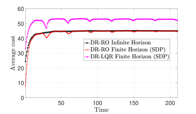
(a) White noise

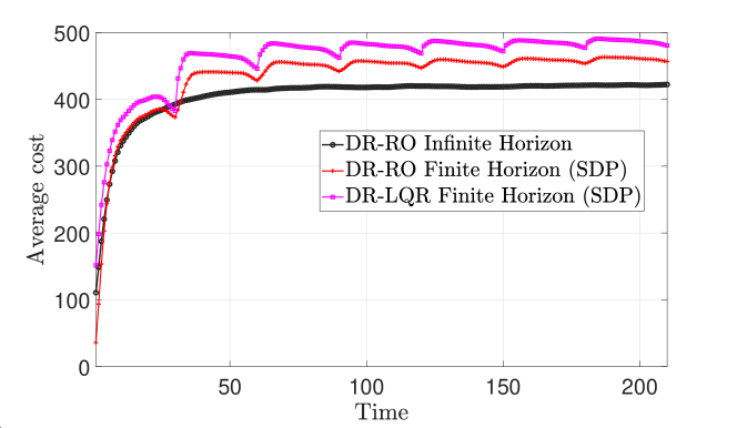
(b) Worst disturbance for (I)

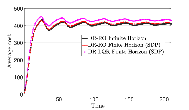
(c) Worst disturbance for (II)

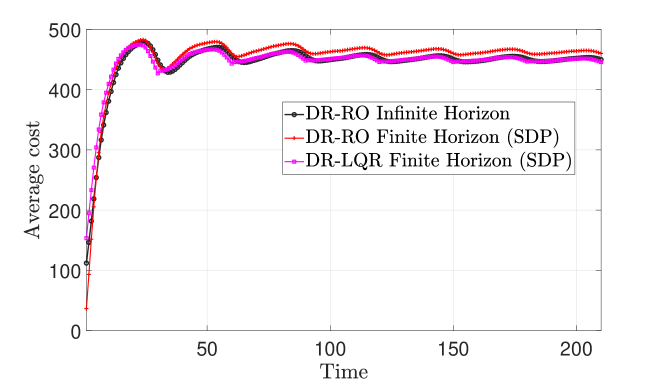
(d) Worst disturbance for (III)

Figure 4: The control costs of the different DR controllers: (I) DR-RO in infinite horizon, (II) DR-RO in finite horizon and (III) DR-LQR in finite horizon under different disturbances for system [REA4] (Leibfritz & Lipinski, 2003). (a) is white noise, while (b), (c) and (d) are worst-case disturbances for each of the controllers, for $r=1.5$. The finite-horizon controllers are re-applied every $s=30$ steps. For all disturbances, the infinite horizon DRRO controller achieves lowest average cost, even in cases (c) and (d) where the finite horizon DR controllers are designed to minimize the cost.

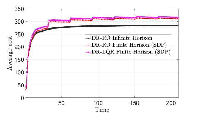
(a) White noise

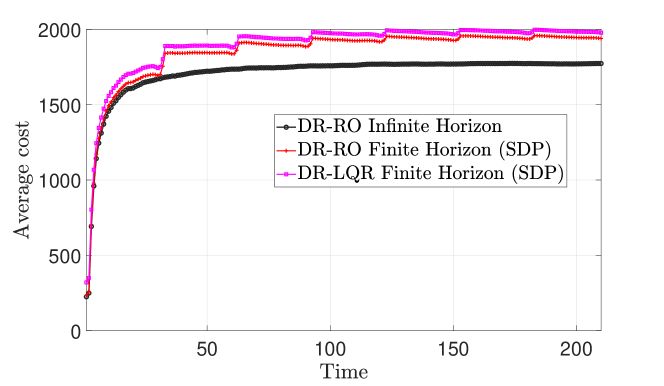
(b) Worst disturbance for (I)

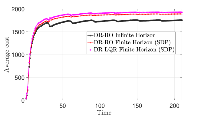
(c) Worst disturbance for (II)

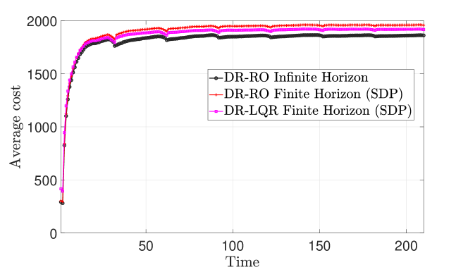
(d) Worst disturbance for (III)

Figure 5: The control costs of the different DR controllers: (I) DR-RO in infinite horizon, (II) DR-RO in finite horizon and (III) DR-LQR in finite horizon under different disturbances for system [HE3] (Leibfritz & Lipinski, 2003). (a) is white noise, while (b), (c) and (d) are worst-case disturbances for each of the controllers, for $r=1.5$. The finite-horizon controllers are re-applied every $s=30$ steps. For all disturbances, the infinite horizon DRRO controller achieves lowest average cost, even in cases (c) and (d) where the finite horizon DR controllers are designed to minimize the cost.

In figures 6 and 7, we show the performance of the different DR controllers: (I) DR-RO in infinite horizon, (II) DR-RO in finite horizon and (III) DR-LQR in finite horizon under uniform noise and sinusoidal noise, respectively, for different systems. Note that the distributionally robust controller is guaranteed to perform better than other controllers under its own worst-case distribution, but has no guarantee of performance under other disturbances. Under uniform and sinusoidal noise, our infinite horizon DR-RO controller performs better than the finite horizon DR-LQR for systems [REA4] and [AC15], but worse than the finite horizon DR-LQR and on par with the finite horizon DR-RO for system [HE3].

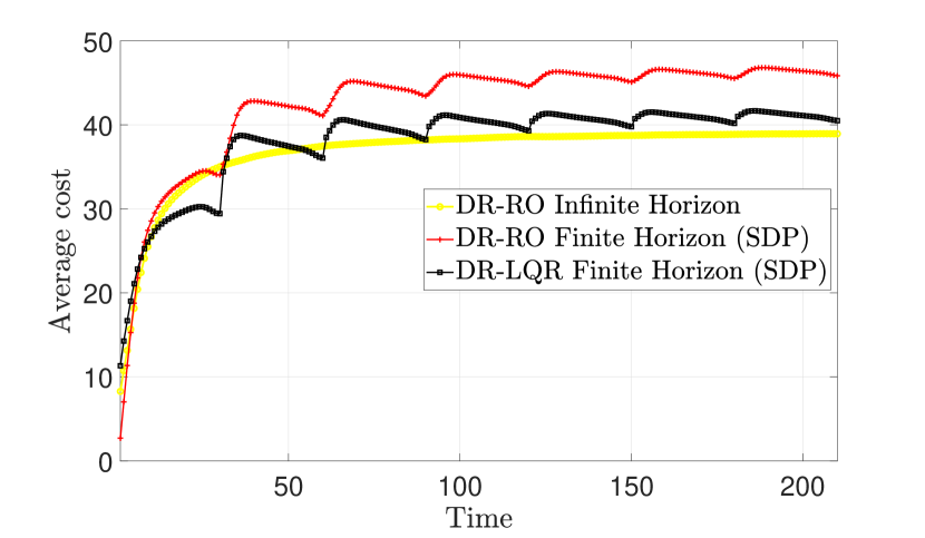
(a) System [REA4]

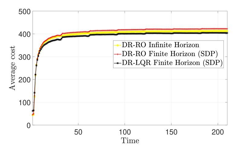
(b) System [HE3]

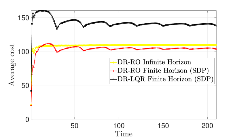
(c) System [AC15]

Figure 6: The control costs of the different DR controllers: DR-RO in infinite horizon, DR-RO in finite horizon and DR-LQR in finite horizon under uniform noise distributions (with amplitude=2) for different systems, for $r=1.5$.

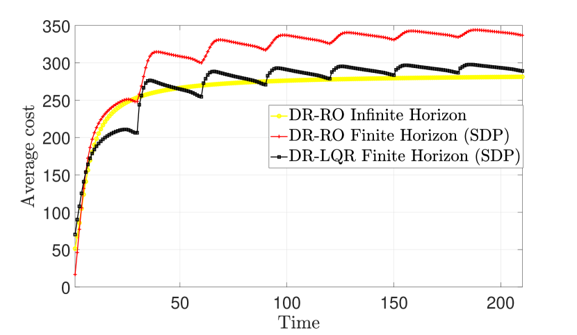
(a) System [REA4]

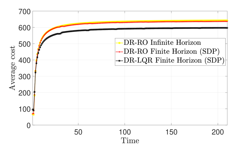
(b) System [HE3]

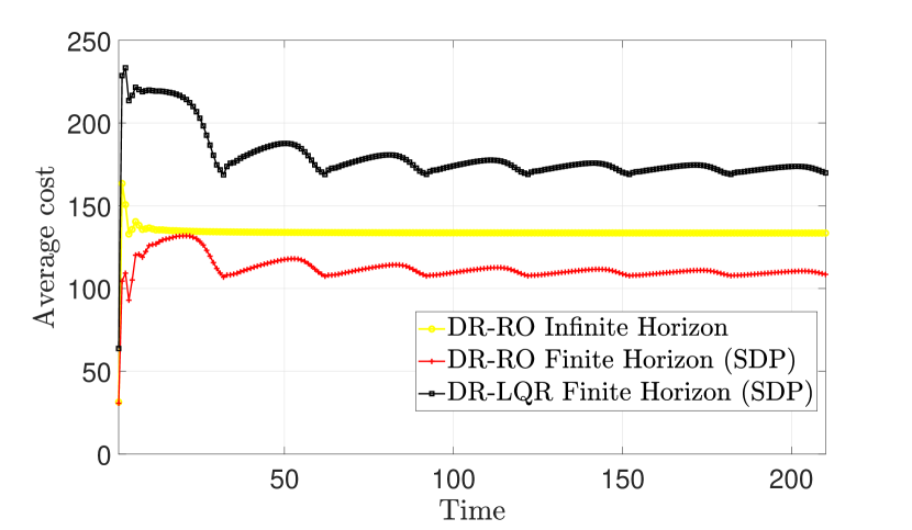
(c) System [AC15]

Figure 7: The control costs of the different DR controllers: DR-RO in infinite horizon, DR-RO in finite horizon and DR-LQR in finite horizon under sinusoidal noise distributions (frequency=1, phase=$\pi/4$, amplitude=2) for different systems, for $r=1.5$.

Frequency domain simulations

We show in figure 8 the frequency domain representation of the square of the norm of the DR-RO controller and its approximation for [AC15] and [HE3], demonstrating that lower order approximations of $m(e^{j\omega})$ provide good estimates.

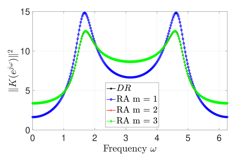
(a)

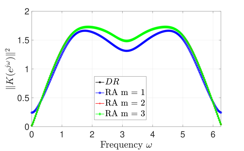
(b)

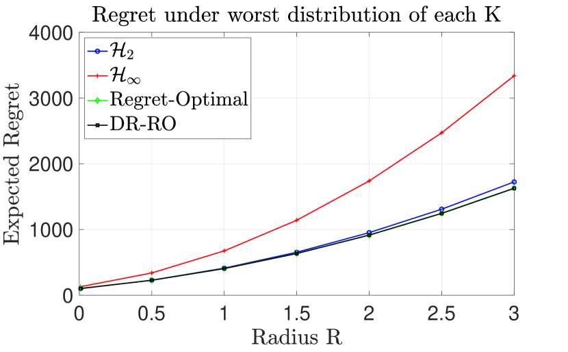
(c)

Figure 8: The frequency domain representation of the square of the norm of the DR-RO controller $K(e^{jw})$ and its approximation for [AC15] 8(a) and [HE3] 8(b). Figures 8(a) and 8(b) reaffirm our conclusions that lower order approximations of $m(e^{jw})$ still yield good estimates of the same. Figure 8(c) represents the worst case expected regret of $\mathcal{H}_{2},\mathcal{H}_{\infty}$ and the RO controller.

References

• Aolaritei et al. (2023a) Aolaritei, L., Fochesato, M., Lygeros, J., and Dörfler, F. Wasserstein tube mpc with exact uncertainty propagation. In 2023 62nd IEEE Conference on Decision and Control (CDC), pp.  2036–2041, 2023a. doi: 10.1109/CDC49753.2023.10383526.
• Aolaritei et al. (2023b) Aolaritei, L., Lanzetti, N., and Dörfler, F. Capture, propagate, and control distributional uncertainty. In 2023 62nd IEEE Conference on Decision and Control (CDC), pp.  3081–3086, 2023b. doi: 10.1109/CDC49753.2023.10383424.
• Arjovsky et al. (2017) Arjovsky, M., Chintala, S., and Bottou, L. Wasserstein generative adversarial networks. In Precup, D. and Teh, Y. W. (eds.), Proceedings of the 34th International Conference on Machine Learning, volume 70 of Proceedings of Machine Learning Research, pp.  214–223. PMLR, 06–11 Aug 2017.
• Bhatia et al. (2017) Bhatia, R., Jain, T., and Lim, Y. On the Bures-Wasserstein distance between positive definite matrices, December 2017. arXiv:1712.01504 [math].
• Blanchet et al. (2023) Blanchet, J., Kuhn, D., Li, J., and Taskesen, B. Unifying Distributionally Robust Optimization via Optimal Transport Theory, August 2023. arXiv:2308.05414 [math, stat].
• Blau & Michaeli (2019) Blau, Y. and Michaeli, T. Rethinking lossy compression: The rate-distortion-perception tradeoff. In International Conference on Machine Learning, pp.  675–685, Long Beach, California, USA, July 2019. PMLR.
• Brouillon et al. (2023) Brouillon, J.-S., Martin, A., Lygeros, J., Dörfler, F., and Trecate, G. F. Distributionally robust infinite-horizon control: from a pool of samples to the design of dependable controllers, 2023.
• Danskin (1966) Danskin, J. M. The theory of max-min, with applications. SIAM Journal on Applied Mathematics, 14(4):641–664, 1966. ISSN 00361399.
• Didier et al. (2022) Didier, A., Sieber, J., and Zeilinger, M. N. A system-level approach to regret optimal control. IEEE Control Systems Letters, 6:2792–2797, 2022.
• Doyle et al. (1988) Doyle, J., Glover, K., Khargonekar, P., and Francis, B. State-space solutions to standard $h_{2}$ and $h_{\infty}$ control problems. In 1988 American Control Conference, pp.  1691–1696, Atlanta, GA, USA, June 1988. IEEE. doi: 10.23919/ACC.1988.4789992.
• Doyle (1985) Doyle, J. C. Structured uncertainty in control system design. In 1985 24th IEEE Conference on Decision and Control, pp.  260–265, 1985. doi: 10.1109/CDC.1985.268842.
• Dumitrescu (2017) Dumitrescu, B. Positive Trigonometric Polynomials and Signal Processing Applications. Signals and Communication Technology. Springer International Publishing, Cham, 2017. ISBN 978-3-319-53687-3 978-3-319-53688-0. doi: 10.1007/978-3-319-53688-0.
• Ephremidze (2010) Ephremidze, L. An Elementary Proof of the Polynomial Matrix Spectral Factorization Theorem, November 2010. arXiv:1011.3777 [math].
• Ephremidze et al. (2018) Ephremidze, L., Saied, F., and Spitkovsky, I. M. On the Algorithmization of Janashia-Lagvilava Matrix Spectral Factorization Method. IEEE Transactions on Information Theory, 64(2):728–737, February 2018. ISSN 0018-9448, 1557-9654. doi: 10.1109/TIT.2017.2772877.
• Falconi et al. (2022) Falconi, L., Ferrante, A., and Zorzi, M. A new perspective on robust performance for LQG control problems. In 2022 IEEE 61st Conference on Decision and Control (CDC), pp.  3003–3008, Cancun, Mexico, December 2022. IEEE. ISBN 978-1-66546-761-2. doi: 10.1109/CDC51059.2022.9992567.
• Frank & Wolfe (1956) Frank, M. and Wolfe, P. An algorithm for quadratic programming. Naval Research Logistics Quarterly, 3(1-2):95–110, March 1956. ISSN 0028-1441, 1931-9193. doi: 10.1002/nav.3800030109.
• Gao & Kleywegt (2022) Gao, R. and Kleywegt, A. J. Distributionally Robust Stochastic Optimization with Wasserstein Distance, April 2022. arXiv:1604.02199 [math].
• Goel & Hassibi (2021a) Goel, G. and Hassibi, B. Regret-optimal measurement-feedback control. In Learning for Dynamics and Control, pp.  1270–1280. PMLR, 2021a.
• Goel & Hassibi (2021b) Goel, G. and Hassibi, B. Regret-optimal control in dynamic environments, February 2021b. arXiv:2010.10473 [cs, eess, math].
• Goel & Hassibi (2023) Goel, G. and Hassibi, B. Regret-optimal estimation and control. IEEE Transactions on Automatic Control, 68(5):3041–3053, 2023.
• Goldstein (1964) Goldstein, A. A. Convex programming in Hilbert space. Bulletin of the American Mathematical Society, 70(5):709 – 710, 1964.
• Hajar et al. (2023a) Hajar, J., Kargin, T., and Hassibi, B. Wasserstein Distributionally Robust Regret-Optimal Control under Partial Observability. In 2023 59th Annual Allerton Conference on Communication, Control, and Computing (Allerton), pp.  1–6, Monticello, IL, USA, September 2023a. IEEE. ISBN 9798350328141. doi: 10.1109/Allerton58177.2023.10313386.
• Hajar et al. (2023b) Hajar, J., Sabag, O., and Hassibi, B. Regret-Optimal Control under Partial Observability, November 2023b. arXiv:2311.06433 [cs, eess, math].
• Hakobyan & Yang (2022) Hakobyan, A. and Yang, I. Wasserstein distributionally robust control of partially observable linear systems: Tractable approximation and performance guarantee. In 2022 IEEE 61st Conference on Decision and Control (CDC), pp.  4800–4807. IEEE, 2022.
• Hansen & Sargent (2008) Hansen, L. and Sargent, T. Robustness. Princeton University Press, 2008. ISBN 978-0-691-11442-2.
• Hassibi et al. (1999) Hassibi, B., Sayed, A. H., and Kailath, T. Indefinite-Quadratic Estimation and Control. Society for Industrial and Applied Mathematics, 1999. doi: 10.1137/1.9781611970760.
• Hu & Hong (2012) Hu, Z. and Hong, L. J. Kullback-Leibler divergence constrained distributionally robust optimization, November 2012.
• Jacobson (1973) Jacobson, D. Optimal stochastic linear systems with exponential performance criteria and their relation to deterministic differential games. IEEE Transactions on Automatic Control, 18(2):124–131, April 1973. ISSN 0018-9286. doi: 10.1109/TAC.1973.1100265.
• Jaggi (2013) Jaggi, M. Revisiting Frank-Wolfe: Projection-Free Sparse Convex Optimization. In Dasgupta, S. and McAllester, D. (eds.), Proceedings of the 30th International Conference on Machine Learning, volume 28 of Proceedings of Machine Learning Research, pp.  427–435, Atlanta, Georgia, USA, June 2013. PMLR. Issue: 1.
• Kailath et al. (2000) Kailath, T., Sayed, A. H., and Hassibi, B. Linear estimation. Prentice Hall information and system sciences series. Prentice Hall, Upper Saddle River, N.J, 2000. ISBN 978-0-13-022464-4.
• Kalman (1960) Kalman, R. E. A New Approach to Linear Filtering and Prediction Problems. Journal of Basic Engineering, 82(1):35–45, March 1960. ISSN 0021-9223. doi: 10.1115/1.3662552.
• Kargin et al. (2023) Kargin, T., Hajar, J., Malik, V., and Hassibi, B. Wasserstein Distributionally Robust Regret-Optimal Control in the Infinite-Horizon, December 2023. arXiv:2312.17376 [cs, eess, math].
• Kim & Yang (2023) Kim, K. and Yang, I. Distributional robustness in minimax linear quadratic control with wasserstein distance. SIAM Journal on Control and Optimization, 61(2):458–483, 2023. doi: 10.1137/22M1494105.
• Kuhn et al. (2019) Kuhn, D., Esfahani, P. M., Nguyen, V. A., and Shafieezadeh-Abadeh, S. Wasserstein distributionally robust optimization: Theory and applications in machine learning. In Operations research & management science in the age of analytics, pp.  130–166. Informs, 2019.
• Lacoste-Julien & Jaggi (2014) Lacoste-Julien, S. and Jaggi, M. An Affine Invariant Linear Convergence Analysis for Frank-Wolfe Algorithms, January 2014. arXiv:1312.7864 [math].
• Lei et al. (2021) Lei, E., Hassani, H., and Bidokhti, S. S. Out-of-distribution robustness in deep learning compression. arXiv preprint arXiv:2110.07007, October 2021.
• Leibfritz & Lipinski (2003) Leibfritz, F. and Lipinski, W. Description of the benchmark examples in compleib 1.0. Dept. Math, Univ. Trier, Germany, 32, 2003.
• Liu et al. (2023) Liu, R., Shi, G., and Tokekar, P. Data-driven distributionally robust optimal control with state-dependent noise. In 2023 IEEE/RSJ International Conference on Intelligent Robots and Systems (IROS), pp.  9986–9991, 2023. doi: 10.1109/IROS55552.2023.10342392.
• Liu et al. (2020) Liu, Y., Zhu, L., Yamada, M., and Yang, Y. Semantic Correspondence as an Optimal Transport Problem. In 2020 IEEE/CVF Conference on Computer Vision and Pattern Recognition (CVPR), pp.  4462–4471, Seattle, WA, USA, June 2020. IEEE. ISBN 978-1-72817-168-5. doi: 10.1109/CVPR42600.2020.00452.
• Lotidis et al. (2023) Lotidis, K., Bambos, N., Blanchet, J., and Li, J. Wasserstein Distributionally Robust Linear-Quadratic Estimation under Martingale Constraints. In Ruiz, F., Dy, J., and van de Meent, J.-W. (eds.), Proceedings of The 26th International Conference on Artificial Intelligence and Statistics, volume 206 of Proceedings of Machine Learning Research, pp.  8629–8644. PMLR, April 2023.
• Malik et al. (2024) Malik, V., Kargin, T., Kostina, V., and Hassibi, B. A Distributionally Robust Approach to Shannon Limits using the Wasserstein Distance, May 2024. arXiv:2405.06528 [cs, math].
• Martin et al. (2022) Martin, A., Furieri, L., Dorfler, F., Lygeros, J., and Ferrari-Trecate, G. Safe control with minimal regret. In Learning for Dynamics and Control Conference, pp.  726–738. PMLR, 2022.
• Martinelli et al. (2023) Martinelli, D., Martin, A., Ferrari-Trecate, G., and Furieri, L. Closing the Gap to Quadratic Invariance: a Regret Minimization Approach to Optimal Distributed Control, November 2023. arXiv:2311.02068 [cs, eess].
• Ozaydin et al. (2024) Ozaydin, B., Zhang, T., Bhattacharjee, D., Süsstrunk, S., and Salzmann, M. OMH: Structured Sparsity via Optimally Matched Hierarchy for Unsupervised Semantic Segmentation, April 2024. arXiv:2403.06546 [cs].
• Petersen et al. (2000) Petersen, I., James, M., and Dupuis, P. Minimax optimal control of stochastic uncertain systems with relative entropy constraints. IEEE Transactions on Automatic Control, 45(3):398–412, March 2000. ISSN 00189286. doi: 10.1109/9.847720.
• Prabhat & Bhattacharya (2024) Prabhat, H. and Bhattacharya, R. Optimal State Estimation in the Presence of Non-Gaussian Uncertainty via Wasserstein Distance Minimization, March 2024. arXiv:2403.13828 [cs, eess, math, stat].
• Rino (1970) Rino, C. Factorization of spectra by discrete Fourier transforms (Corresp.). IEEE Transactions on Information Theory, 16(4):484–485, July 1970. ISSN 0018-9448. doi: 10.1109/TIT.1970.1054502.
• Sabag & Hassibi (2022) Sabag, O. and Hassibi, B. Regret-Optimal Filtering for Prediction and Estimation. IEEE Transactions on Signal Processing, 70:5012–5024, 2022. ISSN 1053-587X, 1941-0476. doi: 10.1109/TSP.2022.3212153.
• Sabag et al. (2021) Sabag, O., Goel, G., Lale, S., and Hassibi, B. Regret-optimal controller for the full-information problem. In 2021 American Control Conference (ACC), pp.  4777–4782. IEEE, 2021.
• Sabag et al. (2023) Sabag, O., Goel, G., Lale, S., and Hassibi, B. Regret-optimal lqr control, 2023.
• Samuelson & Yang (2017) Samuelson, S. and Yang, I. Data-driven distributionally robust control of energy storage to manage wind power fluctuations. In 2017 IEEE Conference on Control Technology and Applications (CCTA), pp.  199–204, 2017. doi: 10.1109/CCTA.2017.8062463.
• Sayed & Kailath (2001) Sayed, A. H. and Kailath, T. A survey of spectral factorization methods. Numerical Linear Algebra with Applications, 8(6-7):467–496, September 2001. ISSN 1070-5325, 1099-1506. doi: 10.1002/nla.250.
• Shafieezadeh Abadeh et al. (2018) Shafieezadeh Abadeh, S., Nguyen, V. A., Kuhn, D., and Mohajerin Esfahani, P. M. Wasserstein distributionally robust kalman filtering. In Bengio, S., Wallach, H., Larochelle, H., Grauman, K., Cesa-Bianchi, N., and Garnett, R. (eds.), Advances in Neural Information Processing Systems, volume 31. Curran Associates, Inc., 2018.
• Sharon et al. (2021) Sharon, N., Peiris, V., Sukhorukova, N., and Ugon, J. Flexible rational approximation and its application for matrix functions. arXiv preprint arXiv:2108.09357, 2021.
• Speyer et al. (1974) Speyer, J., Deyst, J., and Jacobson, D. Optimization of stochastic linear systems with additive measurement and process noise using exponential performance criteria. IEEE Transactions on Automatic Control, 19(4):358–366, August 1974. ISSN 0018-9286. doi: 10.1109/TAC.1974.1100606.
• Taha et al. (2023) Taha, F. A., Yan, S., and Bitar, E. A Distributionally Robust Approach to Regret Optimal Control using the Wasserstein Distance. In 2023 62nd IEEE Conference on Decision and Control (CDC), pp.  2768–2775, Singapore, Singapore, December 2023. IEEE. ISBN 9798350301243. doi: 10.1109/CDC49753.2023.10384311.
• Taskesen et al. (2023) Taskesen, B., Iancu, D., Kocyigit, C., and Kuhn, D. Distributionally robust linear quadratic control. In Oh, A., Naumann, T., Globerson, A., Saenko, K., Hardt, M., and Levine, S. (eds.), Advances in Neural Information Processing Systems, volume 36, pp.  18613–18632. Curran Associates, Inc., 2023.
• Tzortzis et al. (2015) Tzortzis, I., Charalambous, C. D., and Charalambous, T. Dynamic programming subject to total variation distance ambiguity. SIAM Journal on Control and Optimization, 53(4):2040–2075, 2015. doi: 10.1137/140955707.
• Tzortzis et al. (2016) Tzortzis, I., Charalambous, C. D., Charalambous, T., Kourtellaris, C. K., and Hadjicostis, C. N. Robust Linear Quadratic Regulator for uncertain systems. In 2016 IEEE 55th Conference on Decision and Control (CDC), pp.  1515–1520, Las Vegas, NV, USA, December 2016. IEEE. ISBN 978-1-5090-1837-6. doi: 10.1109/CDC.2016.7798481.
• van der Grinten (1968) van der Grinten, P. M. E. M. Uncertainty in measurement and control. Statistica Neerlandica, 22(1):43–63, 1968. doi: https://doi.org/10.1111/j.1467-9574.1960.tb00617.x.
• Villani (2009) Villani, C. Optimal transport: old and new. Number 338 in Grundlehren der mathematischen Wissenschaften. Springer, Berlin, 2009. ISBN 978-3-540-71049-3. OCLC: ocn244421231.
• Whittle (1981) Whittle, P. Risk-sensitive linear/quadratic/gaussian control. Advances in Applied Probability, 13(4):764–777, December 1981. ISSN 0001-8678, 1475-6064. doi: 10.2307/1426972.
• Wiener & Hopf (1931) Wiener, N. and Hopf, E. Über eine Klasse singulärer Integralgleichungen. Sitzungsberichte der Preussischen Akademie der Wissenschaften. Physikalisch-mathematische Klasse. Akad. d. Wiss., 1931.
• Wilson (1972) Wilson, G. T. The Factorization of Matricial Spectral Densities. SIAM Journal on Applied Mathematics, 23(4):420–426, 1972. ISSN 00361399. doi: 10.1137/0123044. Publisher: Society for Industrial and Applied Mathematics.
• Yan et al. (2023) Yan, S., Taha, F. A., and Bitar, E. A distributionally robust approach to regret optimal control using the wasserstein distance, 2023.
• Yang (2020) Yang, I. Wasserstein distributionally robust stochastic control: A data-driven approach. IEEE Transactions on Automatic Control, 66(8):3863–3870, 2020.
• Youla et al. (1976) Youla, D., Jabr, H., and Bongiorno, J. Modern Wiener-Hopf design of optimal controllers–Part II: The multivariable case. IEEE Transactions on Automatic Control, 21(3):319–338, June 1976. ISSN 0018-9286. doi: 10.1109/TAC.1976.1101223.
• Zames (1981) Zames, G. Feedback and optimal sensitivity: Model reference transformations, multiplicative seminorms, and approximate inverses. IEEE Transactions on Automatic Control, 26(2):301–320, April 1981. ISSN 0018-9286. doi: 10.1109/TAC.1981.1102603.
• Zhao & Guan (2018) Zhao, C. and Guan, Y. Data-driven risk-averse stochastic optimization with Wasserstein metric. Operations Research Letters, 46(2):262–267, March 2018. ISSN 01676377. doi: 10.1016/j.orl.2018.01.011.
• Zhong & Zhu (2023) Zhong, Z. and Zhu, J.-J. Nonlinear wasserstein distributionally robust optimal control. In ICML Workshop on New Frontiers in Learning, Control, and Dynamical Systems, 2023.
• Zhou et al. (1996) Zhou, K., Doyle, J. C., and Glover, K. Robust and optimal control. Prentice Hall, Upper Saddle River, N.J, 1996. ISBN 978-0-13-456567-5.