A generic and robust quantum agent inspired by deep meta-reinforcement learning

Abstract

Deep reinforcement learning (deep RL) has enabled human- or superhuman- performances in various applications. Recently, deep RL has also been adopted to improve the performance of quantum control. However, a large volume of data is typically required to train the neural network in deep RL, making it inefficient compared with the traditional optimal quantum control method. Here, we thus develop a new training algorithm inspired by the deep meta-reinforcement learning (deep meta-RL), which requires significantly less training data. The trained neural network is adaptive and robust. In addition, the algorithm proposed by us has been applied to design the Hadamard gate and show that for a wide range of parameters the infidelity of the obtained gate can be made of the order $10^{-4}$. Our algorithm can also automatically adjust the number of pulses required to generate the target gate, which is different from the traditional optimal quantum control method which typically fixes the number of pulses a-priory. The results of this paper can pave the way towards constructing a universally robust quantum agent catering to the different demands in quantum technologies.

I Introduction

Recent theoretical and experimental studies have shown that quantum phenomena, such as entanglement and superposition, can be used to facilitate quantum technologies in computing, communications and information storage to outperform the classical counterpart[1, 2, 3]. Quantum control is fundamental to the realization of these emerging technologies, and it also plays an important method for studying areas such as atomic physics and physical chemistry[4, 5].

Quantum control is usually implemented by manipulating the Hamiltonians of quantum systems. By applying a series of unitary transformations driven by the control Hamiltonians to the target system, the target system can be transferred to desired states. How to obtain such a control sequence, especially the optimal scheme, is a core problem to be addressed by quantum control. A variety of control algorithms have been proposed in the past few decades, and have achieved excellent results in specific models. For example, the gradient ascent pulse engineering (GRAPE) method [6], widely used in quantum optimal control, which takes advantage of the gradient-based optimization of a model-based target function.

However, in reality there inevitably exist noises or inaccuracies in the information flow of quantum control systems, including but not limited to output limitations of the actuators[7], sensor measurement errors[8], interactions with the environment, and approximations of the physical models[9]. These factors can significantly influence quantum control systems with high precision requirements. For instance, regarding the application of GRAPE, limited knowledge about the system dynamics and control Hamiltonians means that GRAPE may result in control deviations and even uncontrollability. Although early search algorithms like gradient ascent (GA) exhibit some robustness, they are in need of a large amount of time to optimize algorithm performance and are susceptible to falling into local optimal solutions (see e.g. [6]). Therefore, designing an efficient algorithm to address uncertainty remains an important research direction in quantum control systems.

It is widely shared that machine learning (ML) has seen rapid progress in recent years. ML learns from data or interactions and can efficiently and accurately perform classification or optimization tasks [10]. Furthermore, the combination of ML and quantum control systems has been gradually explored [11, 12]. Leveraging the advantages of ML, the need for accurately modeling quantum system dynamics has been eliminated, thereby improving the control performance in different scenarios. In particular, since reinforcement learning (RL) in ML has been extensively applied in the regime of classical control, the integration of RL into quantum control has become a hot topic, which is anticipated to lead to remarkable achievements.

There are indeed a number of recent works utilizing the techniques of RL [13], including value-based[14, 15, 16] and policy gradient-based[17, 18] algorithms, to discover quantum optimal control strategies. RL mainly consists of two basic components: the environment and the agent. The environment is typically established based on specific task requirements, such as games[19] and optimization problems[20], while the agent is responsible for the decision-making process within the task and learns the optimal policy. Through interactions with the environment, the agent can update its policy accordingly. However, existing results have indicated that deep RL has at least two drawbacks compared to human-beings. On the one hand, training an intelligent agent requires a massive amount of data, while humans can achieve reasonable performance in a novel environment with significantly less data. This limitation is particularly critical in quantum optimal control problems, as the exponential growth in the size of quantum states leads to a rapid decline in the sample efficiency, which thus brings a challenge to RL. On the other hand, deep RL typically specializes in a narrow task domain, while humans can effortlessly apply knowledge acquired from other scenarios to the current task.

In recent years, research has focused on task transfer in RL, such as transfer RL[21] and meta-RL[22], which have improved the generalization of reinforcement learning algorithms across different tasks.

Therefore, inspired by deep meta-RL, in this paper we propose a new scheme which provides a generic and robust quantum agent that can adapt to different parameters in quantum systems. This scheme significantly reduces the training time required for a quantum agent to handle diverse task environments, and facilitates the transition of the algorithm among different control environments. Since quantum gates serve as the fundamental operational elements in quantum computing[23], achieving high-fidelity quantum gates is of the utmost importance for ensuring the accuracy and efficiency in the vast majority of quantum technologies. It is worth mentioning that the algorithm proposed by us has been applied to design the Hadamard gate with high fidelity obtained. To be specific, for a wide range of parameters, the infidelity of the realized gate can be reduced to be of the order $10^{-4}$. In addition, our algorithm can automatically adjust the number of control pulses required to generate the target gate, different from the traditional optimal quantum control method which typically fixes the number of pulses a-priory. Furthermore, we show that the pulses generated by our agent at a fixed point is more robust than the pulses generated by GRAPE.

II Methods

Since deep reinforcement learning (deep RL), which combines reinforcement learning (RL) and deep learning, can outperform human-beings in complex decision making problems, it has attracted much attention. In this section, we describe how the RL problem can be formalized as an agent that has to make decisions in an environment to optimize a given notion of cumulative rewards. Before presenting the formal setting, we introduce the mathematical concept of a Markov decision process. A Markov decision process (MDP) can be defined by a 5-tuple $(\mathcal{S},\mathcal{A},T,R,\gamma)$, satisfying

• $\mathcal{S}$ is the state space;

• $\mathcal{A}$ is the action space;

• $T:\mathcal{S}\times\mathcal{A}\times\mathcal{A}\to[0,1]$ is the transition function;

• $R:\mathcal{S}\times\mathcal{A}\times\mathcal{S}\to\mathcal{R}$, where $\mathcal{R}$ is a continuous set of possible reward;

• $\gamma$ is a discounted factor.

As shown in the yellow loop of Fig. 1, the general RL setting is formulated as a process where the agent interacts with the external environment in the following way.

Namely, the agent (shown by the blue brain in Fig. 1) takes the action $a_{t}$ at the time $t$, leading to three consequences. Firstly, the agent receives a reward $r_{t}$. Secondly, the state of the environment transmits from $s_{t}$ to $s_{t+1}$. Thirdly, the agent receive a new observation $s_{t+1}$. If the agent is required to have a good memory in certain circumstances, a recurrent loop will be added to formulate the agent’s brain, depicted by the closed gray arrow in Fig. 1.

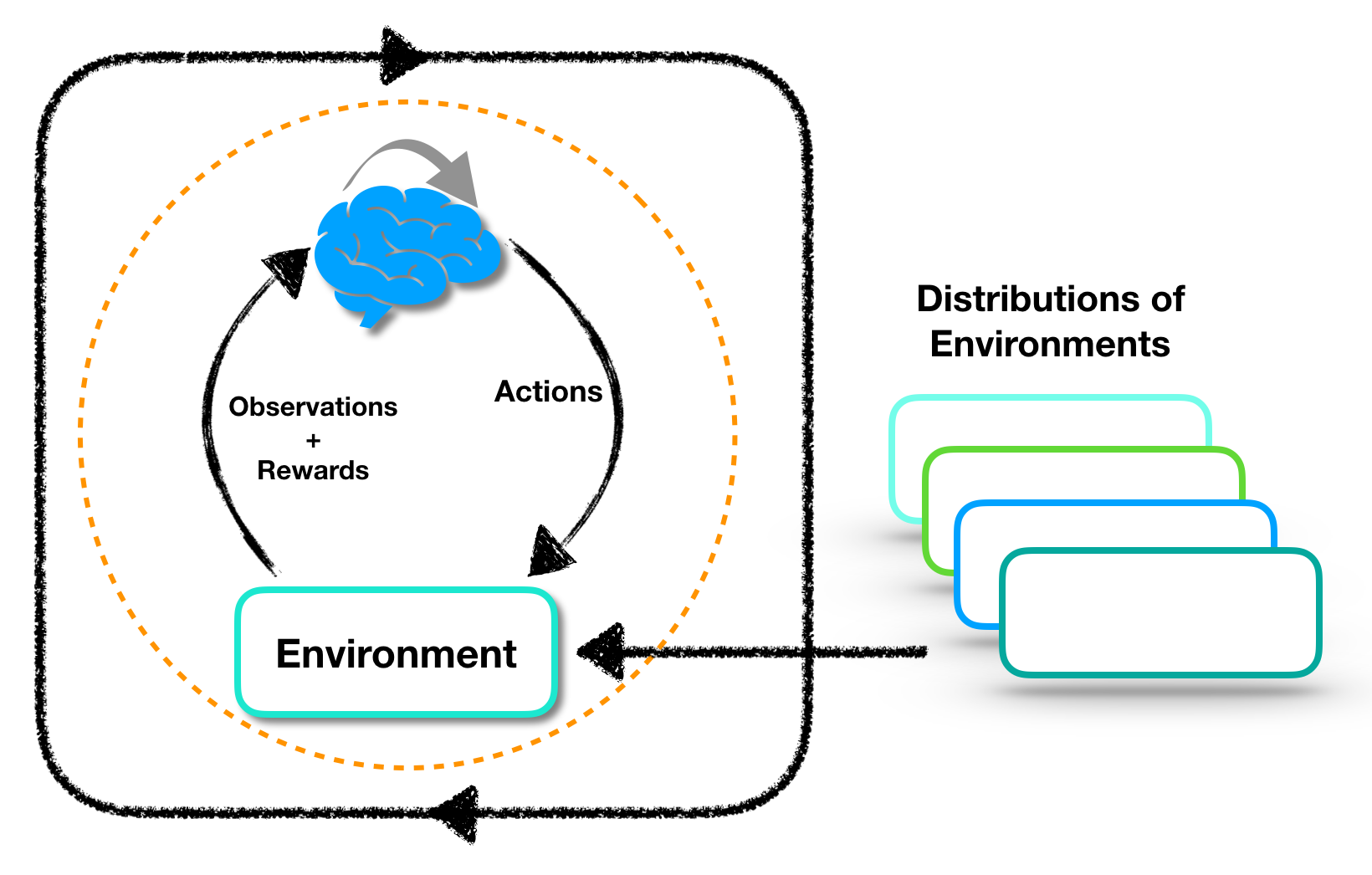
Figure 1: This figure shows the framework of metaQctrl. The yellow loop denotes the general setting of a MDP. The agent takes action $a_{t}$ at the time $t$ based on the observation $s_{t}$, and it brings three consequences: 1) a reward $r_{t}$ is received; 2) the state of environment transmits from $s_{t}$ to $s_{t+1}$; 3) a new observation $s_{t+1}$ is gained.

Throughout this process, the agent aims to find a policy $\pi(a|s)$ to optimize the total expected reward that can be obtained, referred to the following reward function defined by

$$J(\theta)=\sum_{s\in\mathcal{S}}d^{\pi}(s)V^{\pi}(s)=\sum_{s\in\mathcal{S}}d^{\pi}(s)\sum_{a\in\mathcal{A}}\pi_{\theta}(a|s)Q^{\pi}(s,a),$$ (1)

where,

$$V^{\pi}(s)=\mathbb{E}_{a\sim\pi}[\sum_{k\geq 0}\gamma^{k}R_{t+k}|S_{t}=s],$$ (2)

$$Q^{\pi}(s,a)=\mathbb{E}[\sum_{k\geq 0}\gamma^{k}R_{t+k}|S_{t}=s,a_{t}=a],$$ (3)

and $d^{\pi}(s)$ is the stationary distribution of the Markov chain defined by $d^{\pi}(s)=\lim_{t\to\infty}P(s_{t}=s|s_{0},\pi)$. The policy-based reinforcement learning algorithm aims at optimizing this policy $\pi$ directly, and it is approximated by a neural network $\pi_{\theta}$, where $\theta$ is the core parameter in this approximator. Based on this setting, one can expect that policy gradient methods are more powerful when the state or action space is continuous, because one can save a table with infinite values according to the tabular method. Moreover, in the generalized policy iteration, the policy improvement $\arg\max_{a}Q^{\pi}(s,a)$ requires us to traverse the whole state space, which is impossible for the continuous action space. This phenomenon is called the curse of dimensionality. In order to update the reward function, one is supposed to compute the associated gradient according to the policy gradient theorem, namely

$$\nabla_{\theta}J(\theta) =\nabla_{\theta}\sum_{s\in\mathcal{S}}d^{\pi}(s)\sum_{a\in\mathcal{A}}\pi_{\theta}(a|s)Q^{\pi}(s,a)$$ (4)

$$\propto\sum_{s\in\mathcal{S}}d^{\pi}(s)\sum_{a\in\mathcal{A}}Q^{\pi}(s,a)\nabla_{\theta}\pi_{\theta}(a|s).$$

Eq. (4) makes calculation of the gradient independent from the derivatives of $d^{\pi}$ and $Q^{\pi}(s,a)$.

A canonical quantum control problem, i.e. generation of the Hadamard gate, is considered here to demonstrate our algorithm in detail. More concretely, given the control Hamiltonian as follows,

$$H(t)=\eta(u_{x}(t)\sigma_{x}+u_{y}(t)\sigma_{y}),$$ (5)

our goal is to find the optimal pulses $\vec{u}(t):=(u_{x}(t),u_{y}(t))$ evolving the identity operator $I$ to $U_{f}=\frac{\sigma_{x}+\sigma_{z}}{\sqrt{2}}$, where $\sigma_{x},\sigma_{y},\sigma_{z},I$ are Pauli matrices defined by $\sigma_{x}=\left(\begin{array}[]{cc}0&1\\ 1&0\end{array}\right),\sigma_{y}=\left(\begin{array}[]{cc}0&-i\\ i&0\end{array}\right),\sigma_{z}=\left(\begin{array}[]{cc}1&0\\ 0&-1\end{array}\right)$, $I=\left(\begin{array}[]{cc}1&0\\ 0&1\end{array}\right)$. In this quantum gate generation problem, we take the maximal total time $T=2$, duration of each slice $dt=\frac{T}{N}$, where $N=50$ denotes the maximal number of pulses, and the parameter $\eta$ samples from the clipped Gaussian distribution $\mathrm{clip}(\mathcal{N}(0.5,0.2),0.3,0.7)$. The objective is to maximize the following fidelity and find the optimal pulse $\vec{u}^{*}_{\eta}$,

$$\mathcal{U}^{*}=\arg\max_{\mathcal{U}}\int d\eta\mathcal{F}(U(T,\vec{u}_{\eta}),U),$$ (6)

where $U(T)=\mathcal{T}e^{-i\int_{0}^{T}d\tau H(\tau)}$. Here $\mathcal{F}$ is the norm square of fidelity between two gates, i.e. $\mathcal{F}=\frac{1}{4}|\mathrm{Tr}[U(T)U_{f}^{{\dagger}}]|^{2}$, representing the objective function. It is worth noting that the formulation of $\mathcal{U}^{*}$ is quite different from the stereotype considered in tradition quantum control problems. In previous studies, researchers tend to find the optimal control pulse $\vec{u}^{*}_{\eta}$ for a given $\eta$ such that $\mathcal{F}(U(T),U_{f})$ moves as close to $1$ as they can. In our approach, a general map $\mathcal{U}^{*}:\eta\to\vec{u}^{*}_{\eta}$ will be found instead of solving the former concrete problem, which is thus more complicated than obtaining the solution for a fixed given $\eta$. Or rather say, if an algorithm such as GRAPE is employed to find $\vec{u}_{\eta}^{*}$, then one needs to run the algorithm each time a new sample is encountered. Therefore it is time-consuming to iterate for thousands of rounds. However, our algorithm only makes use of one training episode to complete the optimization, allowing for a post-trained neural network, which is generic for $\eta$ in a wide range. Then we simply need to simulate the following process in a cycle: 1) feeding the current quantum gate $U(t)$ into a post-trained neural network, which outputs the pulse $\vec{u}(t)$; 2) evolving the current quantum gate $U(t)$ to $U(t+dt)$ via the propagator $e^{-i\eta dt\vec{u}(t)\cdot\vec{\sigma}}$.

We now give a brief instruction on how the quantum agent in our work can be trained. We denote the scheme where the agent is trained at a fixed $\eta$ ($\eta=0.5$) as RLQctrl (inspired by reinforcement learning to explore the quantum control strategy for short), and the scheme where the agent is trained by the distributions of $\eta$ as metaQctrl (inspired by meta reinforcement learning to explore the quantum control strategy for short). For the metaQctrl agent, we train it by two steps inspired by meta-RL, which would be expounded in the following.

• Sample $\eta\sim\mathrm{clip}(\mathcal{N}(0.5,0.2),0.3,0.7)$, and obtain the dynamics driven by $H(t)=\eta\vec{u}(t)\cdot\vec{\sigma}$.

• For this fixed $\eta$, sample data chain $s_{0}\stackrel{{\scriptstyle a_{0}}}{{\longrightarrow}}(s_{1},r_{0})\stackrel{{\scriptstyle a_{1}}}{{\longrightarrow}}(s_{2},r_{1})\stackrel{{\scriptstyle a_{2}}}{{\longrightarrow}}\cdots\stackrel{{\scriptstyle a_{N-1}}}{{\longrightarrow}}(s_{N},r_{N-1})$. Here each action $a_{t}$ is guided by the policy network, in the way it is sampled from a normal distribution with the mean $\mu_{t}$ and the standard variance $\sigma_{t}$ output by the agent.

With the data collected, one can compute the value loss and the policy loss as well as their gradients obtained by auto-gradient softwares, such as Pytorch, in order to minimize these losses. Deep meta-RL is inclined to use a recurrent network to enhance the memory ability of an agent by feeding $(a_{t-1},r_{t-1},s_{t})$ to the network work as a tuple. The reason why a recurrent network is not needed will be explained in the rest of this section. Since the task dynamics are modeled by a MDP in the reinforcement learning setting, the information chain $s_{0}\to s_{1}\to\cdots\to s_{N}$ can not completely recover the whole process including $(a_{t},r_{t})$. The Markov process, determined by the distribution $T:\mathcal{S}\times\mathcal{A}\times\mathcal{A}\to[0,1]$, thus plays a critical role in this setting. However, in the quantum optimal control problem, $r_{t-1}$ is exactly given by the fidelity between $s_{t}$ and $U_{f}$. We can then derive the control pulse $a_{t-1}$ by calculating the propagator from $s_{t-1}$ to $s_{t}$. Hence, given the state transition chain, we can know the whole information of this gate generation process, which means our agent has memory of this design procedure. Consequently, only fully connective network has been used in our architecture, as shown in Fig.2. The green nodes are vectorized representation of the quantum gate. Two purple hidden layers are used to encode such representation, after which two linear layers (the policy and value layers) are considered. The policy and value layers are constructed with the purpose of decoding and obtaining the approximators $\pi(a_{t}|s_{t},\theta)$ and $V(s_{t},\theta_{v})$, where $\theta$ and $\theta_{v}$ are parameters in the policy and value functions.

Figure 2: Architecture of the neural network considered in our work. Input is vectorized representation of a quantum gate, and then two hidden layers are used to encode this state. Finally, two types of decoders are used to generate the policy and value functions respectively.

III Results

For the generation of a single-qubit quantum gate, it can be seen that both RLQctrl and metaQctrl converge when we run $4000$ epochs, as shown in Fig.3. Furthermore, we can find that metaQctrl is able to deal with explore-exploit trade-off much better than RLQctrl. For a fixed value of $\eta$, the quantum gates that the agent experiences are trapped by this single value. By contrast, for distributed values of $\eta$,the diversity of quantum gates emerged in our sampled data is much larger than the former, indicating that the agent can get more information about a global landscape and has a wider horizon for the feasible control region. This can be verified by the oscillation of policy loss and faster convergence of value loss, which thus explains why metaQctrl can outperform RLQctrl in the following results.

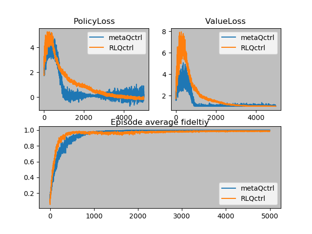
Figure 3: This figure shows the agent training process for both RLQctrl and metaQctrl, including how policy loss, value loss, and average episode fidelity vary when training epochs increase.

On the one hand, Fig. 4 illustrates that metaQctrl can perform quite well in the systems with new parameters which do not appear in the training process. Specifically, we can find from Fig. 4 that:

• metaQctrl is better than RLQctrl when $\eta$ takes values varying from $0.25$ to $2.0$.

• When $\eta$ decreases, it can be observed that the quantum fidelities of both metaQctrl and RLQctrl reduce and that the corresponding decay rate of RLQctrl is larger than that of metaQctrl.

Moreover, it can be observed from Fig. 4 that the infildelity experiences rapid decay for $\eta\in(0.25,0.29)$, which indicates that the total time $T=2$ approaches the quantum speed limit in this scenario. And we numerically The critical point of $\eta$ for the total time $T=2$ with respect to the number of slices $N=50$ is around $0.26$.

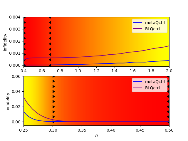
Figure 4: The x-axis is value of $\eta$ and y-axis is infidelity. The purple line denote agent trained at a fixed $\eta=0.5$ and the blue line denote the agent trained from a MDP distribution obeying $\mathrm{clip}(\mathcal{N}(0.5,0.2),0.3,0.7)$, which lie in the region between such black arrows.

On the other hand, apart from the universality of our agent, we will show that the agent can adjust number of pulses for different problems. It is widely shared that time and energy are conjugate physical quantities, and therefore the same effect can be achieved by either increasing the time (quantified by the number of pulses) or decreasing the allowable energy (quantified by the value of $\eta$). We plot the number of pulses required to generate the Hadamard gate with the quantum fidelities achieved at least $0.999$ by metaQctrl and RLQctrl in Fig. 5. In more concrete terms, it can be concluded that:

• The agents, including the ones trained by metaQctrl and RLQctrl, can adjust the number of pulses adaptively according to different system parameters.

• The agents can reveal the conjugate relation between energy and time. Although this property might seem trivial for physicists, it implies that the quantum agent may discover intrinsic and fundamental principles to a certain extent when it is trained for relevant engineering problems.

• The agent trained by metaQctrl takes less pluses to achieve the same fidelity for a fixed $\eta$ than the agent trained by RLQctrl does, which means pulses provided by metaQctrl is more effective than those provided by RLQctrl. This is due to the fact that metaQctrl has a wider control horizon and a stronger ability to balance the explore-exploit trade-off as mentioned above.

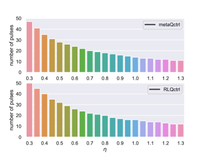
Figure 5: The x-axis shows discrete values of $\eta=0.3,0.35,0.4,\cdots,1.25,1.3$, and the y-axis shows the number of pulses to obtain the fidelity up to at least $0.999$. The upper and lower sub-figures show the corresponding results given by the agents trained by metaQctrl and RLQctrl respectively.

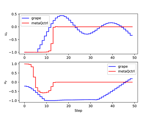
Figure 6: This figure shows the shape of pulses when $\eta=1$, $T=2$ and number of slices $N=50$ for metaQctrl and GRAPE respectively.

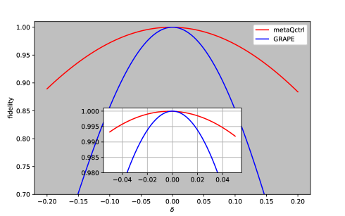
Figure 7: This figure shows the fidelity when the values of $\eta=1+\delta$ vary, according to the robust control strategy.

The robustness of our quantum agent can also be further explored. In practice, there inevitably exists noise in open quantum systems. For example, in magnetic resonance experiments, the spins may suffer from large dispersion in the applied electric field strength (radio-frequency in-homogeneity). A canonical problem in quantum control is thus to develop strategies which are robust to such disturbance in realistic experiments. In order to convey more clearly, we rewrite our Hamiltonian as follows,

$$H=\eta(u_{x}\sigma_{x}+u_{y}\sigma_{y})=(1+\delta)(u_{x}\sigma_{x}+u_{y}\sigma_{y}),$$ (7)

where $\delta$ denotes the signal noise ratio (SNR) for pulses. Firstly a set of pulses are generated by using both metaQctrl and GRAPE for fixed $\eta=1$, as plotted in Fig. 7. Then, we apply these pulses to the noisy system with the SNR $\delta$. According to Fig.7, it can be seen that metaQctrl always perform better than GRAPE does when there is disturbance in the system. Besides, the strength of pulses gained by metaQctrl vanishes when the step number is larger than $16$, while GRAPE uses the total number of steps ($50$ steps) converging to the local solution by ignoring its surroundings in terms of the feasible control landscape. This proves that the quantum agent trained by metaQctrl has a global horizon. More precisely, compared to GRAPE, mataQctrl tends to converge to a global optimum instead of trapping in an extremely local valley.

IV Discussions

In this paper, we propose a training scheme inspired by deep meta-RL. In contrast to previous research combining reinforcement learning and quantum control, we add an outer loop sampling quantum dynamics from prior distribution of system parameters.The sample efficiency has been remarkably increased during the data collection process, and the agent has been offered a wider horizon in terms of the control landscape. This thus brings in three prominent advantages, namely universality, adaptiveness, and robustness. In particular, compared to the agent trained at a fixed point, metaQctrl has stronger generalization ability when new system parameters are encountered. The self-adjusting capacity uncovers conjugate relation between energy and time, which is learnt by the agent itself without any relevant guide. Last but not least, a wider horizon enables our agent to generate more robust and effective pulses. Future work may include the generation of multiple-qubit quantum gates by constructing a universally robust quantum agent catering to the different demands.

References

- [1] M. A. Nielsen and I. L. Chuang, Quantum Computation and Quantum Information. Cambridge University Press, 2011.
- [2] F. Xia, J. Liu, H. Nie, Y. Fu, L. Wan, and X. Kong, “Random walks: A review of algorithms and applications,” IEEE Transactions on Emerging Topics in Computational Intelligence, vol. 4, no. 2, pp. 95–107, 2020.
- [3] H. Khabat, G. E. Duncan, C. H. Peter, and J. B. Philip, “Quantum memories: emerging applications and recent advances,” Journal of Modern Optics, vol. 63, no. 20, pp. 2005–2028, 2016.
- [4] S. Chu, “Cold atoms and quantum control,” Nature, vol. 416, no. 6877, p. 206–210, 2002.
- [5] D. Dong and I. R. Petersen, “Quantum control theory and applications: a survey,” IET Control Theory and Applications, vol. 4, no. 12, pp. 2651–2671, 2010.
- [6] N. Khaneja, T. Reiss, C. Kehlet, T. Schulte-Herbrüggen, and S. J. Glaser, “Optimal control of coupled spin dynamics: design of nmr pulse sequences by gradient ascent algorithms,” Journal of Magnetic Resonance, vol. 172, no. 2, pp. 296–305, 2005.
- [7] H.-J. Ding and R.-B. Wu, “Robust quantum control against clock noises in multiqubit systems,” Phys. Rev. A, vol. 100, no. 2, pp. 022302–022308, 2019.
- [8] I. N. Hincks, C. E. Granade, T. W. Borneman, and D. G. Cory, “Controlling quantum devices with nonlinear hardware,” Phys. Rev. A, vol. 4, no. 2, pp. 024012–024020, 2015.
- [9] H. Wang, Y. Ding, J. Gu, Y. Lin, D. Z. Pan, F. T. Chong, and S. Han, “Quantumnas: Noise-adaptive search for robust quantum circuits,” in 2022 IEEE International Symposium on High-Performance Computer Architecture, pp. 692–708, 2022.
- [10] A. Shrestha and A. Mahmood, “Review of deep learning algorithms and architectures,” IEEE Access, vol. 7, pp. 53040–53065, 2019.
- [11] Z. Wang and C. Guet, “Deep learning in physics: A study of dielectric quasi-cubic particles in a uniform electric field,” IEEE Transactions on Emerging Topics in Computational Intelligence, vol. 6, no. 3, pp. 429–438, 2022.
- [12] S. Y.-C. Chen, C.-H. H. Yang, J. Qi, P.-Y. Chen, X. Ma, and H.-S. Goan, “Variational quantum circuits for deep reinforcement learning,” IEEE Access, vol. 8, pp. 141007–141024, 2020.
- [13] X.-M. Zhang, Z. Wei, R. Asad, X.-C. Yang, and X. Wang, “When does reinforcement learning stand out in quantum control? a comparative study on state preparation,” npj Quantum Information, vol. 5, pp. 85–92, 2019.
- [14] M. Bukov, A. G. R. Day, D. Sels, P. Weinberg, A. Polkovnikov, and P. Mehta, “Reinforcement learning in different phases of quantum control,” Phys. Rev. X, vol. 8, pp. 031086–031101, Sep 2018.
- [15] S. Hu, C. Chen, and D. Dong, “Deep reinforcement learning for control design of quantum gates,” in 2022 13th Asian Control Conference, pp. 2367–2372, 2022.
- [16] H. Ma, D. Dong, S. X. Ding, and C. Chen, “Curriculum-based deep reinforcement learning for quantum control,” IEEE Transactions on Neural Networks and Learning Systems, vol. 34, no. 11, pp. 8852–8865, 2023.
- [17] L. Moro, M. G. A. Paris, M. Restelli, and E. Prati, “Quantum compiling by deep reinforcement learning,” Commun Phys, vol. 4, no. 1, p. 178, 2021.
- [18] C. Jiang, Y. Pan, Z.-G. Wu, Q. Gao, and D. Dong, “Robust optimization for quantum reinforcement learning control using partial observations,” Phys. Rev. A, vol. 105, no. 6, pp. 062443–062455, 2022.
- [19] K. Shao, Y. Zhu, and D. Zhao, “Starcraft micromanagement with reinforcement learning and curriculum transfer learning,” IEEE Transactions on Emerging Topics in Computational Intelligence, vol. 3, no. 1, pp. 73–84, 2019.
- [20] Z. Pan, L. Wang, J. Wang, and J. Lu, “Deep reinforcement learning based optimization algorithm for permutation flow-shop scheduling,” IEEE Transactions on Emerging Topics in Computational Intelligence, vol. 7, no. 4, pp. 983–994, 2023.
- [21] A. Taylor, I. Dusparic, M. Guériau, and S. Clarke, “Parallel transfer learning in multi-agent systems: What, when and how to transfer?,” in 2019 International Joint Conference on Neural Networks, pp. 1–8, 2019.
- [22] C. Finn, P. Abbeel, and S. Levine, “Model-agnostic meta-learning for fast adaptation of deep networks,” in International Conference on Machine Learning, 2017.
- [23] A. Y. Kitaev, “Quantum computations: algorithms and error correction,” Russian Mathematical Surveys, vol. 52, no. 6, p. 1191, 1997.