Probabilistic Time Integration for Semi-explicit PDAEs^∗

Abstract.

This paper deals with the application of probabilistic time integration methods to semi-explicit partial differential–algebraic equations of parabolic type and its semi-discrete counterparts, namely semi-explicit differential–algebraic equations of index $2$. The proposed methods iteratively construct a probability distribution over the solution of deterministic problems, enhancing the information obtained from the numerical simulation. Within this paper, we examine the efficacy of the randomized versions of the implicit Euler method, the midpoint scheme, and exponential integrators of first and second order. By demonstrating the consistency and convergence properties of these solvers, we illustrate their utility in capturing the sensitivity of the solution to numerical errors. Our analysis establishes the theoretical validity of randomized time integration for constrained systems and offers insights into the calibration of probabilistic integrators for practical applications.

Key words. PDAEs, semi-explicit systems, probabilistic numerics, randomization
AMS subject classifications. 65M12, 65J15, 65L80

1. Introduction

Over the past few years, randomized time integration methods for ordinary differential equations have been studied extensively; see [CCCG16, CGS⁺17, LSS19, AG20, LSS22]. These methods aim to statistically quantify the uncertainty introduced by the time discretization. For this, classical probabilistic solvers iteratively establish a probability measure over the numerical solution of deterministic initial value problems of the form

(1.1) $$\dot{u}(t)=f(t,u(t)),\qquad u(0)=u^{0}\in\mathbb{R}^{d},$$

offering more comprehensive information than a single (deterministic) solve. Let $\psi_{t}\colon[0,T]\times\mathbb{R}^{d}\rightarrow\mathbb{R}^{d}$ denote the flow map induced by (1.1), meaning that $u(t)=\psi_{t}(0,u^{0})$. On the other hand, a numerical one-step method can be expressed by a mapping $\Psi_{t}\colon[0,T]\times\mathbb{R}^{d}\rightarrow\mathbb{R}^{d}$ with

$$u^{n+1}=\Psi_{\tau}(t^{n},u^{n}),\qquad n=0,1,\dots,$$

assuming an equidistant partition with $t^{n}=n\tau$ and time step size $\tau$. Here, $u^{n}$ denotes the approximation of $u(t^{n})=\psi_{n\tau}(t^{0},u^{0})$. Typically, these methods produce a single discrete solution, often accompanied by some form of an error indicator. However, they do not fully quantify the remaining uncertainty in the path statistically. In order to capture the sensitivity of the solution to numerical errors, while maintaining consistent convergence properties from classical deterministic integrators, the probabilistic interpretation of the numerical solution introduced in [CGS⁺17] considers the randomized scheme

$$U^{n+1}=\Psi_{\tau}(t^{n},U^{n})+\xi^{n}(\tau),\qquad n=0,1,\dots$$

with $U^{0}=u^{0}$ and appropriately scaled independent and identically distributed (i.i.d.) random variables $\xi^{n}(\tau)$ with values in $\mathbb{R}^{d}$. This then results in a sequence of random variables $U^{n}$ approximating $u(t^{n})$. We would like to emphasize that probabilistic integrators may neither inherently provide more accurate solutions than classical deterministic methods, nor are they necessarily computationally cheaper. They prove useful, however, in statistical inference settings, particularly in tasks such as integrating chaotic dynamical systems and solving Bayesian inverse problems [CCCG16].

The purpose of this paper is to address the construction and rigorous analysis of probabilistic time integration methods for constrained systems. Besides, we consider the operator case leading to so-called partial differential–algebraic equations (PDAEs); see [LMT13] for an introduction. To be more precise, we consider a (semi-linear) parabolic system

$$\dot{u}(t)+\mathcal{A}u(t)=f(t,u)$$

together with a linear constraint of the form $\mathcal{B}u(t)=g(t)$ included by the Lagrangian method, cf. [EM13, Alt15]. In the corresponding semi-discretized setting, i.e., after the application of a spatial discretization scheme, this yields a semi-explicit differential–algebraic equation (DAE) of index $2$; see [HW96, Ch. VII.1].

Known deterministic time stepping methods for such DAEs and PDAEs include algebraically stable Runge–Kutta methods [HLR89, KM06, AZ18], splitting methods [AO17], (discontinuous) Galerkin methods [VR19, AH21], and exponential integrators [AZ20]. In this study, we provide a framework how to randomize existing (deterministic) integration schemes, including the specific construction of four randomized methods. We identify assumptions and introduce a local random field, particularly a Gaussian field, to reflect the uncertainty. The resulting probabilistic solvers allow for repeated sampling in order to explore the solutions uncertainty. In the following example, we illustrate the difficulty arising for constrained systems and the consequences of perturbations affecting the constraint; see also [ALM17].

Example 1.1.

To illustrate the randomized idea from [CGS⁺17], let us consider the FitzHugh–Nagumo model [RHCC07] with an additional constraint. With the help of the Lagrangian method, we obtain the nonlinear system

$$\dot{V}(t)=3\,V(t)-V^{3}(t)+3\,R(t)-\lambda(t),\qquad\dot{R}(t)=\frac{-5\,V(t)+1-R(t)}{15}-\lambda(t)$$

with the constraint $V(t)+R(t)=\sin(t)$ and unknowns $V$, $R$, and $\lambda$. As initial conditions, we set $V(0)=-1$ and $R(0)=1$. When a small perturbation is added to the constraint, implemented as a scalar Gaussian random variable $\varepsilon\sim\mathcal{N}(0,\sigma^{2})$, this leads to chaotic behavior. As a result, the trajectories strongly deviate from the true solution. However, if we add perturbations only in the dynamic part, one can see that every probabilistic solution is a good approximation of the exact solution. In Figure 1.1, we present $50$ trajectories for the $V$ species computed by the implicit Euler scheme with $\sigma=0.1$, once affecting the constraint and once only acting on the dynamic part of the solution. This illustrates the sensitivity of the solution to perturbations on the constraint. On the other hand, Figure 1.2 depicts $50$ trajectories for the $V$ species for different noise scales $\sigma$, showing the sensitivity of the solutions with respect to $\sigma$. At this point, we would like to emphasize that the scale parameter $\sigma$ should, in general, be chosen problem-dependent on basis of specific characteristics of the model. Such a calibration controls the apparent uncertainty in the solver and is discussed later on.

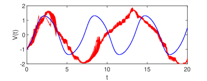
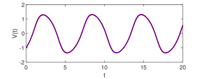
Figure 1.1. The exact trajectory of $V$ of the constrained FitzHugh–Nagumo model from Example 1.1 (blue) and $50$ trajectories (red) obtained by the implicit Euler method with Gaussian perturbation on the constraint (left) and on the dynamic part only (right). In both cases the noise scale equals $\sigma=0.1$.

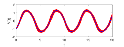
Figure 1.2. Exact value of $V$ (blue) and $50$ trajectories (red) in the same setting as in Figure 1.1 with different noise scales, namely $\sigma=0.5$ (left) and $\sigma=1.5$ (right).

In the forthcoming section, we introduce the model of interest and the necessary setup for the construction of probabilistic integrators. The mean square convergence is then analyzed in Section 3. In Section 4, we delve into the construction of four specific integrators, namely the implicit Euler method, the midpoint scheme, and two exponential integrators of first and second order. To confirm the theoretical findings, we provide a numerical example. Finally, Section 5 is devoted to the calibration of the parameter $\sigma$ when employing randomized time integrators for constrained parabolic systems. Here, we demonstrate that an appropriately scaling enables the randomized solvers to yield probabilistic solutions without affecting the convergence of the corresponding deterministic scheme.

Notation

Given $N\in\mathbb{N}$, we define $[N]\coloneqq\{1,\ldots,N\}$ as well as $[N]_{0}\coloneqq[N]\cup\{0\}$. Moreover, given discrete time points $t^{n}$ and a (continuous) function $g$, we write $g^{n}\coloneqq g(t^{n})$.

2. Preliminaries

In this section, we present the main assumptions and notations that will be used throughout the remainder of this work.

2.1. Semi-explicit (P)DAEs

Within this section, we introduce the model of interest, namely (semi-linear) parabolic systems with linear constraints. Note that this is a PDAE, since the corresponding semi-discrete system, which is obtained by the application of a spatial discretization, equals a semi-explicit DAE of index $2$. More precisely, we consider following task: seek abstract functions $u\colon[0,T]\to\mathcal{V}$ and $\lambda\colon[0,T]\to\mathcal{Q}$ such that

(2.1a) $$\dot{u}(t) \,+\, \mathcal{A}u(t) \,+\, \mathcal{B}^{\ast}\lambda(t)\, =f(t,u) \qquad\text{in }\mathcal{V}^{*},$$

(2.1b) $$\mathcal{B}u(t) =g(t) \qquad\text{in }\mathcal{Q}^{*}$$

is satisfied for almost every $t\in[0,T]$. Moreover, we assume given initial data $u(0)=u^{0}$, which should be consistent in the sense that $\mathcal{B}u^{0}=g(0)$. Within this paper, we assume that $\mathcal{V}$ and $\mathcal{Q}$ are given Hilbert spaces. Together with the dual space $\mathcal{V}^{*}$, we further assume the existence of a Gelfand triple $\mathcal{V},\mathcal{H},\mathcal{V}^{*}$; see [Zei90, Ch. 23.4]. For the involved operators, we mainly follow the assumptions stated in [AZ20].

Assumption 2.1.

The constraint operator $\mathcal{B}\colon\mathcal{V}\to\mathcal{Q}^{*}$ is linear, continuous, and satisfies an inf–sup condition, i.e., there exists a constant $\beta>0$ such that

$$\adjustlimits{\inf}_{q\in\mathcal{Q}\setminus\{0\}}{\sup}_{v\in\mathcal{V}\setminus\{0\}}\frac{\langle\mathcal{B}v,q\rangle}{\|v\|_{\mathcal{V}}\|q\|_{\mathcal{Q}}}\geq\beta.$$

Assumption 2.2.

The differential operator $\mathcal{A}\colon\mathcal{V}\to\mathcal{V}^{*}$ is linear, continuous, and elliptic on $\mathcal{V}_{\ker}\coloneqq\ker\mathcal{B}$, i.e., on the kernel of the constraint operator. Restricted to the kernel, we denote the operator by $\mathcal{A}_{\ker}\coloneqq\mathcal{A}|_{\mathcal{V}_{\ker}}\colon\mathcal{V}_{\ker}\to\mathcal{V}_{\ker}^{*}\coloneqq(\mathcal{V}_{\ker})^{*}$.

Remark 2.3.

The upcoming results can be extended to the situation where $\mathcal{A}$ only satisfies a Gårding inequality on $\mathcal{V}_{\ker}$. In this case, the non-elliptic part can be transferred to the nonlinearity $f$.

Assumption 2.4.

The right-hand sides are assmued to be sufficiently smooth to guarantee the existence of a unique solution. In particular, we assume that $f$ maps into $\mathcal{H}$ and that it is Lipschitz continuous in the second component, i.e., there exists a positive constant $L_{f}$ such that

(2.2) $$\big{\|}f(t,v_{1})-f(t,v_{2})\big{\|}_{\mathcal{H}}\leq L_{f}\,\|v_{1}-v_{2}\|_{\mathcal{H}}.$$

We will also consider corresponding finite-dimensional examples, i.e., semi-explicit DAEs of the form

$$\dot{u}+Au+B^{T}\lambda =f(u),$$

$$Bu\hskip 32.00002pt =g.$$

Here, the assumptions reduce to $B\in\mathbb{R}^{m,n}$ being of full rank and $A\in\mathbb{R}^{n,n}$ being invertible.

We would like to mention two examples which fit into the given framework and which will later be considered in the numerical examples.

Example 2.5.

First, we revisit the constrained FitzHugh–Nagumo model from the introduction. This finite-dimensional example reads

$$\begin{bmatrix}\dot{V}(t)\\ \dot{R}(t)\end{bmatrix}+\begin{bmatrix}-3&-3\\ \tfrac{1}{3}&\tfrac{1}{15}\end{bmatrix}\begin{bmatrix}V(t)\\ R(t)\end{bmatrix}+\begin{bmatrix}1\\ 1\end{bmatrix}\lambda(t) =\begin{bmatrix}-V(t)^{3}\\ \tfrac{1}{15}\end{bmatrix},$$

$$\begin{bmatrix}1&1\end{bmatrix}\begin{bmatrix}V(t)\\ R(t)\end{bmatrix}\hskip 53.49132pt =\sin(t)$$

and is of the considered semi-explicit form. Moreover, the assumed initial conditions $V(0)=-1$, $R(0)=1$ are consistent with the constraint.

Example 2.6.

As a second example, we consider the semi-linear heat equation with a constraint on the integral mean as in [AO17]. More precisely, we consider

(2.3) $$\dot{u}-\Delta u+\mathcal{B}^{*}\lambda=u^{2}\qquad\text{on }\Omega\coloneqq(0,1)$$

with homogeneous Dirichlet boundary conditions for $u$ and the constraint

$$(\mathcal{B}u)(t)\coloneqq\int_{0}^{1}u(x,t)\sin(\pi x)\,\mathrm{d}x=g(t).$$

Here, the operator $\mathcal{A}$ equals the Laplace operator with homogeneous boundary conditions such that Assumption 2.2 is satisfied. Moreover, $\mathcal{B}$ is inf–sup stable, since it is surjective and maps into a finite-dimensional space.

2.2. Decomposition of the solution and flow map

Within the presented setting, it is possible to decompose the solution $u$ into a dynamic part (which lies in the kernel of $\mathcal{B}$) and a complement, which is fully determined by the constraint (2.1b). Due to Assumption 2.1, the constraint operator has a right-inverse $\mathcal{B}^{-}\colon\mathcal{Q}^{*}\to\mathcal{V}$, leading to

$$\mathcal{V}=\mathcal{V}_{\ker}\oplus\mathcal{V}_{\text{c}}\qquad\text{with}\qquad\mathcal{V}_{\ker}=\ker\mathcal{B},\quad\mathcal{V}_{\text{c}}=\operatorname{im}\mathcal{B}^{-}.$$

Following [AZ18], one may choose $\mathcal{V}_{\text{c}}$, e.g., as the annihilator of $\mathcal{V}_{\ker}$. Note that this choice also determines the right-inverse $\mathcal{B}^{-}$. For the resulting decomposition of the solution, we use the notation

$$u=u_{\ker}+u_{c},\qquad u_{\ker}\colon[0,T]\to\mathcal{V}_{\ker},\ u_{c}\colon[0,T]\to\mathcal{V}_{\text{c}}.$$

Inserting this into the constraint (2.1b), we get

$$u_{c}(t)=\mathcal{B}^{-}g(t).$$

The already mentioned consistency condition of the initial data can also be understood in the way that we are only allowed to prescribe $u_{\ker}(0)$. The remaining part $u_{c}(0)$ is determined by $\mathcal{B}^{-}g(0)$ and $\lambda(0)$ can be computed by (2.1a). This motivates the definition of a flow map on the kernel, which we denote by $\psi_{t}\colon[0,T]\times\mathcal{V}_{\ker}\rightarrow\mathcal{V}_{\ker}$. For given $t^{*}\in[0,T]$ with $t^{*}+t\leq T$ and $v_{\ker}\in\mathcal{V}_{\ker}$, this map solves the PDAE (2.1) on the time interval $[t^{*},t^{*}+t]$ with initial data $v_{\ker}+\mathcal{B}^{-}g(t^{*})$. The outcome is then the solution at time $t^{*}+t$ restricted to kernel of $\mathcal{B}$. In particular, we have

(2.4) $$u_{\ker}(t^{n+1})=\psi_{\tau}(t^{n},u_{\ker}(t^{n})).$$

2.3. Deterministic and probabilistic setup

Consider a probability space $(\Omega,\mathcal{F},\mathbb{P})$ that is rich enough to serve as a shared domain for defining all the random variables and processes being studied and let $\mathbb{E}$ denote the expectation with respect to $\mathbb{P}$.

By $\Psi_{\tau}$ we denote a (deterministic) time integration method which can be used to approximate the solution of the semi-explicit system (2.1) or its semi-discretized counterpart. Based on such a scheme, we define a randomized integrator, resulting in a sequence $\{U^{n}\}_{n\in[N]_{0}}$. Each approximation can again be decomposed into

$$U^{n}=U^{n}_{\ker}+U^{n}_{c},\qquad U^{n}_{\ker}\in\mathcal{V}_{\ker},\ U^{n}_{c}\in\mathcal{V}_{\text{c}}.$$

As for the continuous solution, we assume that the approximation at time $t^{n+1}$ is fully determined by $U^{n}_{\ker}$ and the right-hand sides. Hence, we write

(2.5) $$U^{n+1}_{\ker}=\Psi_{\tau}(t^{n},U^{n}_{\ker})+\xi^{n}(\tau),$$

where each $\xi^{n}$ is assumed to be an i.i.d. centred Gaussian random variable with values in $\mathcal{V}_{\ker}$. Since the perturbation only acts on the dynamic part of the solution, the constraint $\mathcal{B}U^{n}=g(t^{n})$ is maintained for all discrete time points. The sequence of errors $e^{n}$ of the random approximation is defined by

$$e^{n}\coloneqq u(t^{n})-U^{n}=u_{\ker}(t^{n})-U_{\ker}^{n},\qquad n\in[N]_{0}.$$

Inserting the definition of the numerical scheme (2.5), we obtain

(2.6) $$e^{n+1}=u_{\ker}(t^{n+1})-\Psi_{\tau}(t^{n},U_{\ker}^{n})-\xi^{n}(\tau),\qquad n\in[N-1]_{0}.$$

The assumptions on the (deterministic) scheme $\Psi_{\tau}$ are summarized in the following.

Assumption 2.7 (Deterministic scheme).

Assume that the time integration scheme $\Psi_{\tau}\colon[0,T]\times\mathcal{V}_{\ker}\rightarrow\mathcal{V}_{\ker}$ meets the following conditions:

• Let $u^{n}_{\ker}$ denote an approximation of $u_{\ker}(t^{n})$ obtained by $\Psi_{\tau}$. Then, there exist constants $\tau^{*},C,q>0$ such that for all step sizes $\tau\in[0,\tau^{*}]$ and $t^{n}\in[0,T]$ it holds that

  (2.7) $$\big{\|}u_{\ker}(t^{n})-u^{n}_{\ker}\big{\|}_{\mathcal{H}}\leq C\,\tau^{q}.$$

• There exist constants $\tau^{*},L_{\Psi}>0$ such that for all step sizes $\tau\in[0,\tau^{*}]$, $t\in[0,T]$, and $v_{1},v_{2}\in\mathcal{V}_{\ker}$ we have the Lipschitz property

  (2.8) $$\big{\|}\Psi_{\tau}(t,v_{1})-\Psi_{\tau}(t,v_{2})\big{\|}_{\mathcal{H}}\leq(1+L_{\Psi}\tau)\,\|v_{1}-v_{2}\|_{\mathcal{H}}.$$

Condition (2.7) corresponds to the convergence order and is essential for the consideration of any deterministic time integration method $\Psi_{\tau}$. The second part of Assumption 2.7 describes a Lipschitz property of the approximate flow map $\Psi_{\tau}$ with respect to its second argument. Next, we state the required assumptions on the random noise, which appears in (2.5).

Assumption 2.8 (Random noise).

The i.i.d. centred Gaussian random variables $\xi^{n}(t)\coloneqq\int_{0}^{t}\chi^{n}(s)\,\mathrm{d}s\in\mathcal{V}_{\ker}$ with $\chi^{n}\sim\mathcal{N}(0,\sigma^{2})$ measured in the $\mathcal{H}$-norm, i.e.,

$$\mathbb{E}\,\|\chi^{n}\|_{\mathcal{H}}=0,\qquad\mathbb{E}\,\|\chi^{n}\|^{2}_{\mathcal{H}}=\sigma^{2},$$

admit parameters $C_{\xi},p>0$ such that for all $t\in[0,\tau]$ it holds that $\mathbb{E}\,\|\xi^{n}(t)\|_{\mathcal{H}}^{2}\leq C_{\xi}\,t^{2p+1}$.

Within the upcoming convergence analysis, we will observe that choosing $p=q$ preserves the strong order of accuracy of the underlying deterministic integrator. This choice introduces the maximum amount of noise consistent with the accuracy of the original deterministic integrator.

3. Mean Square Convergence Analysis

In this section, we analyze the mean square convergence of probabilistic time integration methods for semi-explicit PDAEs of the form (2.1) as introduced in the previous section. We will show that there exists a constant $C>0$ independent of $\tau$ such that

$$\mathbb{E}\,\|u(t^{n})-U^{n}\|_{\mathcal{H}}^{2}\leq C\,\tau^{2r}$$

for all $n\in[N]$. Therein, $r$ is the mean square order of convergence of the method. For the unconstrained case, it is known that $r$ equals to the minimum of $q$ (convergence order of the deterministic time integrator) and $p$ (order of the random noise). Given that our approach is based on a construction in the kernel of the constraint, we expect the same order for the given setting. The analysis of this section will make use of the following inequality.

Lemma 3.1 (Discrete Gronwall lemma).

Suppose that for non-negative sequences $\{x^{{n}}\}_{{n}\in[N]_{0}}$ and $\{y^{{n}}\}_{{n}\in[N]_{0}}$ and for some constant $L>0$, we have $x^{{n}+1}\leq y^{{n}}+(1+\tau L)\,x^{{n}}$ for all $n\in[N-1]_{0}$. Then,

$$x^{n}\leq\bigg{(}x^{0}+\sum_{j=0}^{n-1}\,y^{j}\bigg{)}\exp\big{(}L\tau n\big{)},\qquad{n}\in[N]_{0}.$$

We can now state the global mean square convergence result for probabilistic time integrators applied to (2.1).

Theorem 3.2 (Global mean square convergence).

Let Assumptions 2.1, 2.2, and 2.4 be given. Consider $\tau\leq 1$ and let Assumptions 2.7 and 2.8 hold with orders $q,p>0$, respectively. Then there exists a constant $C>0$ independent of the step size $\tau$ such that

(3.1) $$\sup_{n\in[N]}\big{(}\,\mathbb{E}\,\|u(t^{n})-U^{n}\|^{2}_{\mathcal{H}}\,\big{)}^{1/2}\leq C\,\tau^{\min\{p,q\}}.$$

Proof.

Recall that $U^{n}_{\ker}$ denotes the approximate solution given by the probabilistic solver and let $u_{\ker}^{n}$ denote the corresponding solution given by the underlying deterministic time stepping scheme. For the latter, we define the error

$$\tilde{e}^{n+1}\coloneqq u(t^{n+1})-u^{n+1}=u_{\ker}(t^{n+1})-u_{\ker}^{n+1}=u_{\ker}(t^{n+1})-\Psi_{\tau}(t^{n},u_{\ker}^{n}).$$

Considering the definition of the error $e^{n+1}$ in (2.6) and leveraging the decomposition of the solution $u=u_{\ker}+u_{c}$, we derive

$$\|e^{n+1}-\tilde{e}^{n+1}\|^{2}_{\mathcal{H}} =\big{\|}\Psi_{\tau}(t^{n},u^{n}_{\ker})-\Psi_{\tau}(t^{n},U^{n}_{\ker})-\xi^{n}(\tau)\big{\|}^{2}_{\mathcal{H}}$$

$$=\big{\|}\Psi_{\tau}(t^{n},u^{n}_{\ker})-\Psi_{\tau}(t^{n},U^{n}_{\ker})\big{\|}^{2}_{\mathcal{H}}+\|\xi^{n}(\tau)\|^{2}_{\mathcal{H}}$$

$$\qquad\qquad-2\,\big{(}\Psi_{\tau}(t^{n},u^{n}_{\ker})-\Psi_{\tau}(t^{n},U^{n}_{\ker}),\xi^{n}(\tau)\big{)}_{\mathcal{H}}$$

$$\leq(1+L_{\Psi}\tau)^{2}\|e^{n}-\tilde{e}^{n}\|^{2}_{\mathcal{H}}+\|\xi^{n}(\tau)\|^{2}_{\mathcal{H}}$$

$$\qquad\qquad-2\,\big{(}\Psi_{\tau}(t^{n},u^{n}_{\ker})-\Psi_{\tau}(t^{n},U^{n}_{\ker}),\xi^{n}(\tau)\big{)}_{\mathcal{H}},$$

where Assumption 2.7 was applied in the last step. Now we consider the expectation of this estimate. Since $\xi^{n}$ equals a zero-mean Gaussian random variable, the expectation of the inner product vanishes and we get together with Assumption 2.8

$$\mathbb{E}\,\|e^{n+1}-\tilde{e}^{n+1}\|^{2}_{\mathcal{H}}\leq(1+\tilde{L}_{\Psi}\tau)\,\mathbb{E}\,\|e^{n}-\tilde{e}^{n}\|^{2}_{\mathcal{H}}+C_{\xi}\,\tau^{2p+1},$$

where $\tilde{L}_{\Psi}>0$ is chosen such that $(1+L_{\Psi}\tau)^{2}\leq 1+\tilde{L}_{\Psi}\tau$. Due to $e^{0}=\tilde{e}^{0}=0$, an application of the discrete Gronwall lemma yields

$$\mathbb{E}\,\|e^{n}-\tilde{e}^{n}\|^{2}_{\mathcal{H}}\leq TC_{\xi}\,\tau^{2p}\exp\big{(}\tilde{L}_{\Psi}T\big{)}.$$

Finally, an application of the triangle inequality

$$\mathbb{E}\,\big{\|}e^{n}\big{\|}^{2}_{\mathcal{H}} \leq 2\,\mathbb{E}\,\big{\|}\tilde{e}^{n}\big{\|}^{2}_{\mathcal{H}}+2\,\mathbb{E}\,\big{\|}e^{n}-\tilde{e}^{n}\big{\|}^{2}_{\mathcal{H}},$$

Young’s inequality, and the assumption on the global error of the deterministic solver given in (2.7) yields the desired result. ∎

Remark 3.3.

Condition (2.7) on the order of the deterministic solver may also be replaced by an assumption on the local truncation error. If one assumes a local error of order $q+1$, mean square order of convergence will still be $\min\{p,q\}$. However, the difference between the global and local order of convergence, does not follow the typical pattern observed in deterministic cases. Indeed, the independence of the random variables results in an order reduction of only $1/2$ in the random part of the exponent, while the expected loss of a full order occurs in the deterministic component.

Remark 3.4.

The convergence result of Theorem 3.2 implies that a reasonable option for the noise scale $p$ is to set $p=q$, where $q$ is the order of the underlying deterministic method. This choice of $p$ preserves the convergence of the underlying deterministic method, while providing a probabilistic interpretation of the numerical solution.

4. Examples of Probabilistic Time Integrators

This section is dedicated to exploring randomized time stepping schemes of first and second order for constrained parabolic PDAEs of the form (2.1). For this, we consider four methods in detail and demonstrate how perturbations can be introduced without affecting the constraints of the underlying model. Furthermore, we show that the randomized numerical solution exhibits convergence properties that are asymptotically no inferior to those of the deterministic numerical solution. This implies that the trajectories obtained from the randomized integrator are all equally valid approximations.

4.1. Probabilistic implicit Euler scheme

As a first example, we consider the implicit Euler scheme applied to (2.1). In the deterministic setting, this reads

(4.1a) $$(\operatorname{id}+\tau\mathcal{A})\,u^{n+1}-u^{n}+\tau\mathcal{B}^{*}\lambda^{n+1} =\tau f(t^{n+1},u^{n+1})\qquad\text{in }\mathcal{V}^{*},$$

(4.1b) $$\mathcal{B}u^{n+1}\hskip 80.52135pt =\phantom{\tau}g^{n+1}\hskip 41.82558pt\qquad\text{in }\mathcal{Q}^{*}.$$

Before incorporating perturbations, we discuss Assumption 2.7. It is well-known that the implicit Euler scheme converges with order one without constraints [LO93]. This then directly translates to the solution part in the kernel of the constraint, i.e., we get (2.7) with $q=1$. To prove the Lipschitz property (2.8), we use once more the decomposition of the iterates $u^{n}=u^{n}_{\ker}+u^{n}_{c}$ with $u^{n}_{c}=\mathcal{B}^{-}g^{n}$ as described in Section 2.2. Restricting equation (4.1a) to test functions in $\mathcal{V}_{\ker}$, we get

$$u^{n+1}_{\ker}=u^{n}_{\ker}+\tau\,\big{(}-\mathcal{A}\,u^{n+1}_{\ker}+f(t^{n+1},u_{\ker}^{n+1}+\mathcal{B}^{-}g^{n+1})\big{)}-\mathcal{B}^{-}\big{(}g^{n+1}-g^{n}\big{)}\quad\text{in }\mathcal{V}_{\ker}^{*}$$

and, hence,

$$\Psi_{\tau}(t,v)=v+\tau\,\Big{[}-\mathcal{A}\Psi_{\tau}(t,v)+f\big{(}t+\tau,\Psi_{\tau}(t,v)+\mathcal{B}^{-}g(t+\tau)\big{)}\Big{]}-\mathcal{B}^{-}\big{(}g(t+\tau)-g(t)\big{)}.$$

Lemma 4.1.

Let Assumptions 2.1, 2.2, and 2.4 be given. Then the implicit Euler scheme satisfies the Lipschitz property (2.8).

Proof.

Define

$$w_{1}\coloneqq\Psi_{\tau}(t,v_{1})-\Psi_{\tau}(t,v_{2})\in\mathcal{V}_{\ker},\qquad w_{0}\coloneqq v_{1}-v_{2}\in\mathcal{V}_{\ker}.$$

Rearranging $0\leq\|w_{0}-w_{1}\|^{2}_{\mathcal{H}}$ leads to

$$\tfrac{1}{2\tau}\,\big{(} \|w_{1}\|^{2}_{\mathcal{H}}-\|w_{0}\|^{2}_{\mathcal{H}}\big{)}$$

$$\qquad\leq\tfrac{1}{\tau}\,\big{(}w_{1}-w_{0},w_{1}\big{)}_{\mathcal{H}}$$

$$\qquad\leq-\,\big{\langle}\mathcal{A}w_{1},w_{1}\big{\rangle}_{\mathcal{V}^{*}\times\mathcal{V}}$$

$$\qquad\qquad+\left(f(t,\Psi_{\tau}(t,v_{1})+\mathcal{B}^{-}g(t+\tau))-f(t,\Psi_{\tau}(t,v_{2})+\mathcal{B}^{-}g(t+\tau)),w_{1}\right)_{\mathcal{H}}$$

$$\qquad\leq L_{f}\,\|w_{1}\|^{2}_{\mathcal{H}}.$$

The last estimate follows from the ellipticity of $\mathcal{A}$ on $\mathcal{V}_{\ker}$ and (2.2). We then obtain

$$\|\Psi_{\tau}(t,v_{1})-\Psi_{\tau}(t,v_{2})\|_{\mathcal{H}}\leq(1-2L_{f}\tau)^{-1/2}\|v_{1}-v_{2}\|_{\mathcal{H}},$$

which holds for all $0<\tau\leq\tau^{*}<\tfrac{1}{2L_{f}}$. Setting $L_{\Psi}\coloneqq\tfrac{2L_{f}}{1-2L_{f}\tau^{*}}$, we have

$$(1-2L_{f}\tau)^{-1/2}\leq(1-2L_{f}\tau)^{-1}\leq 1+L_{\Psi}\tau$$

for all $0<\tau\leq\tau^{*}$, which leads to the desired result. ∎

We now turn to the incorporation of perturbations. Here, the precise location of the perturbation is essential in order to ensure that they do not interact with the constraint. Adding the perturbations to the dynamic part, computing one Euler step involves the solution of the saddle point problem

(4.2) $$\begin{bmatrix}\operatorname{id}+\tau\mathcal{A}&\tau\mathcal{B}^{*}\\ \mathcal{B}&0\end{bmatrix}\begin{bmatrix}U^{n+1}\\ \lambda^{n+1}\end{bmatrix}=\begin{bmatrix}U^{n}+\tau f(t^{n+1},U^{n+1})+\xi^{n}(\tau)\\ g^{n+1}\end{bmatrix},$$

where $\xi^{n}(\tau)\in\mathcal{V}_{\ker}$ can be defined as $\sigma\tau^{3/2}\tilde{\xi}^{n}$ by the natural choice of $p=q=1$. Here, $\sigma$ is a constant noise scale and $\tilde{\xi}^{n}$ are i.i.d. standard normal random variables i.e., $\tilde{\xi}^{n}\sim\mathcal{N}(0,1)$. In Section 5, we discuss the case where $\sigma$ is chosen problem-dependent such that the expected order of convergence is maintained.

Remark 4.2.

It is assumed that $\xi^{n}(\tau)\in\mathcal{V}_{\ker}$. Here, however, also $\xi^{n}(\tau)\in\mathcal{V}$ is possible, since the difference would only affect the Lagrange multiplier $\lambda$ and not the constraint.

Remark 4.3.

With an implicit time discretization, one needs to solve a possibly nonlinear system in each time step. This is due to the semi-linear term $f(t^{n+1},U^{n+1})$. This computational burden can be addressed by employing a semi-explicit time stepping method, which implements $f(t^{n},U^{n})$ instead.

4.2. Probabilistic midpoint scheme

The (deterministic) midpoint scheme applied to the PDAE (2.1) results in

(4.3a) $$\big{(}\operatorname{id}+\tfrac{\tau}{2}\mathcal{A}\big{)}\,u^{n+1}-\big{(}\operatorname{id}-\tfrac{\tau}{2}\mathcal{A}\big{)}\,u^{n}+\tau\mathcal{B}^{*}\lambda^{n+1} =\tau f^{n+\frac{1}{2}}\qquad\text{in }\mathcal{V}^{*},$$

(4.3b) $$\mathcal{B}u^{n+1}\hskip 80.52135pt =\phantom{\tau}g^{n+1}\hskip 24.75375pt\text{in }\mathcal{Q}^{*},$$

where $f^{n+\frac{1}{2}}=f\left(t^{n}+\frac{\tau}{2},\frac{1}{2}(u^{n}+u^{n+1})\right)$. The result is a second-order scheme, i.e., we get (2.7) with $q=2$. Using again the fact that $u^{n+1}_{c}=\mathcal{B}^{-}g^{n+1}$ and restricting equation (4.3a) to test functions in $\mathcal{V}_{\ker}$, we obtain

$$\big{(}\operatorname{id}+\tfrac{\tau}{2}\mathcal{A}\big{)}\,u_{\ker}^{n+1}=\big{(}\operatorname{id}-\tfrac{\tau}{2}\mathcal{A}\big{)}\,u^{n}_{\ker}+\tau f\big{(}t^{n}+\tfrac{\tau}{2},\tfrac{1}{2}(u^{n}+u^{n+1})\big{)}-\mathcal{B}^{-}\big{(}g^{n+1}-g^{n}\big{)}\quad\text{in }\mathcal{V}_{\ker}^{*}$$

and, therefore,

$$\Psi_{\tau}(t,v)=\big{(}\operatorname{id}-\tfrac{\tau}{2}\mathcal{A}\big{)}\,v-\tfrac{\tau}{2}\mathcal{A}\Psi_{\tau}(t,v)+\tau f\big{(}t+\tfrac{\tau}{2},v^{*}(t)\big{)}-\mathcal{B}^{-}\big{(}g(t+\tau)-g(t)\big{)}$$

with $v^{*}(t)\coloneqq\frac{1}{2}\big{(}v+\mathcal{B}^{-}g(t)+\Psi_{\tau}(t,v)+\mathcal{B}^{-}g(t+\tau)\big{)}$.

Lemma 4.4.

Let Assumptions 2.1, 2.2, and 2.4 be given. Then the midpoint scheme satisfies the Lipschitz property (2.8).

Proof.

Given $v_{1},v_{2}\in\mathcal{V}_{\ker}$, we define $w_{0}$ and $w_{1}$ as in the proof of Lemma 4.1. It directly follows that $v_{1}^{*}-v_{2}^{*}=\frac{1}{2}(w_{0}+w_{1})$ and, in turn, leads to

$$\tfrac{1}{\tau}\,\big{(}\|w_{1}\|^{2}_{\mathcal{H}}-\|w_{0}\|^{2}_{\mathcal{H}}\big{)} =\tfrac{1}{\tau}\,\big{(}w_{1}-w_{0},w_{0}+w_{1}\big{)}_{\mathcal{H}}$$

$$\leq-\tfrac{1}{2}\,\big{\langle}\mathcal{A}(w_{0}+w_{1}),w_{0}+w_{1}\big{\rangle}_{\mathcal{V}^{*}\times\mathcal{V}}$$

$$\qquad\qquad+\Big{(}f\big{(}t+\tfrac{\tau}{2},v_{1}^{*}\big{)}-f\big{(}t+\tfrac{\tau}{2},v_{2}^{*}\big{)},w_{0}+w_{1}\Big{)}_{\mathcal{H}}$$

$$\leq L_{f}\,\big{(}\|w_{0}\|^{2}_{\mathcal{H}}+\|w_{1}\|^{2}_{\mathcal{H}}\big{)}$$

with the Lipschitz constant $L_{f}>0$ from (2.2). Therefore,

$$\|\Psi_{\tau}(t,v_{1})-\Psi_{\tau}(t,v_{2})\|_{\mathcal{H}}\leq(1-L_{f}\tau)^{-1/2}(1+L_{f}\tau)^{1/2}\,\|v_{1}-v_{2}\|_{\mathcal{H}}$$

for all $0<\tau\leq\tau^{*}<\tfrac{1}{L_{f}}$. Setting $L_{\Psi}\coloneqq\tfrac{2L_{f}}{1-L_{f}\tau^{*}}$, we obtain

$$(1-L_{f}\tau)^{-1/2}(1+L_{f}\tau)^{1/2}\leq 1+L_{\Psi}\tau$$

for all $0<\tau\leq\tau^{*}$, which leads to the desired result. ∎

Similarly as in the previous subsection, by adding perturbations to the dynamic part, computing one step of the midpoint scheme involves solving a saddle point problem of the following form

$$\begin{bmatrix}\operatorname{id}+\frac{\tau}{2}\mathcal{A}&\tau\mathcal{B}^{*}\\ \mathcal{B}&\end{bmatrix}\begin{bmatrix}U^{n+1}\\ \lambda^{n+1}\end{bmatrix}=\begin{bmatrix}(\operatorname{id}-\frac{\tau}{2}\mathcal{A})U^{n}+\tau f^{n+\frac{1}{2}}+\xi^{n}(\tau)\\ g^{n+1}\end{bmatrix},$$

where $\xi^{n}(\tau)\in\mathcal{V}_{\ker}$ can be defined as $\sigma\tau^{5/2}\tilde{\xi}^{n}$ by the natural choice of $p=q=2$, a constant scale $\sigma$ and i.i.d. standard normal random variables $\tilde{\xi}^{n}\sim\mathcal{N}(0,1)$.

4.3. Probabilistic exponential Euler scheme

As third example, we derive the probabilistic version of the exponential Euler method. The corresponding deterministic scheme for constrained systems has been introduced and examined in [AZ20]. Recall that $\mathcal{A}_{\ker}$ denotes the restriction of $\mathcal{A}$ to the kernel of the constraint operator $\mathcal{B}$. Moreover, we introduce $\mathcal{H}_{\ker}$ as the closure of $\mathcal{V}_{\ker}$ in $\mathcal{H}$. Due to Assumption 2.2, we know that $-\mathcal{A}_{\ker}$ generates an analytic semigroup on $\mathcal{H}_{\ker}$; see [Paz83, Ch. 7, Th. 2.7].

Exponential integrators are based on the variation-of-constants formula, which reads

$$u_{\ker}(t^{n+1}) =u(t^{n+1})-\mathcal{B}^{-}g^{n+1}$$

(4.4) $$=e^{-\tau\mathcal{A}_{\ker}}\big{[}u(t^{n})-\mathcal{B}^{-}g^{n}\big{]}+\int_{t^{n}}^{t^{n+1}}e^{-(t^{n+1}-s)\mathcal{A}_{\ker}}\iota_{0}\big{[}f(s,u(s))-\mathcal{B}^{-}\dot{g}(s)\big{]}\,\mathrm{d}s$$

with $\iota_{0}\colon\mathcal{H}\equiv\mathcal{H}^{*}\rightarrow\mathcal{H}^{*}_{\ker}\equiv\mathcal{H}_{\ker}$ denoting the restriction of test functions (which will be omitted from now on). Yet another important tool for the construction are the recursively defined $\varphi$-functions,

(4.5) $$\varphi_{0}(z)\coloneqq e^{z},\qquad\varphi_{k+1}(z)\coloneqq\dfrac{\varphi_{k}(z)-\varphi_{k}(0)}{z}$$

with $\varphi_{k}(0)=1/k!$ for $z=0$. Since $-\mathcal{A}_{\ker}$ generates an analytic semigroup, it follows from [HO10, Lem. 2.4] that $\varphi_{k}(-\tau\mathcal{A}_{\ker})\colon\mathcal{H}_{\ker}\to\mathcal{H}_{\ker}$ defines a bounded operator.

Now, the consideration of suitable quadrature rules in (4.4) leads to exponential integrators. The left-hand rule yields the exponential Euler method as introduced in [AZ20]. It takes the form

(4.6) $$u^{n+1}=\mathcal{B}^{-}g^{n+1}+\varphi_{0}(-\tau\mathcal{A}_{\ker})\big{(}u^{n}-\mathcal{B}^{-}g^{n}\big{)}+\tau\varphi_{1}(-\tau\mathcal{A}_{\ker})\big{(}f(t^{n},u^{n})-\mathcal{B}^{-}\dot{g}^{n}\big{)}.$$

Note that this is an explicit scheme. Considering only the part in the kernel, we get

(4.7) $$\Psi_{\tau}(t,v)=\varphi_{0}(-\tau\mathcal{A}_{\ker})\,v+\tau\varphi_{1}(-\tau\mathcal{A}_{\ker})\big{(}f(t,v+\mathcal{B}^{-}g(t))-\mathcal{B}^{-}\dot{g}(t)\big{)}$$

and it is shown in [AZ20] that this method is of order $q=1$.

Lemma 4.5.

Consider Assumptions 2.1, 2.2, 2.4 and let $\mathcal{A}$ be symmetric. Then the exponential Euler scheme satisfies the Lipschitz property (2.8).

Proof.

A direct calculations shows

$$\big{\|}\Psi_{\tau}(t,v_{1})-\Psi_{\tau}(t,v_{2})\big{\|}_{\mathcal{H}} \leq\big{\|}\varphi_{0}(-\tau\mathcal{A}_{\ker})\,(v_{1}-v_{2})\big{\|}_{\mathcal{H}}$$

$$\qquad+\tau\,\big{\|}\varphi_{1}(-\tau\mathcal{A}_{\ker})\,\big{(}f(t,v_{1}+\mathcal{B}^{-}g(t))-f(t,v_{2}+\mathcal{B}^{-}g(t))\big{)}\big{\|}_{\mathcal{H}}$$

$$\leq\big{(}C_{\varphi_{0}}+\tau\,C_{\varphi_{1}}L_{f}\big{)}\,\big{\|}v_{1}-v_{2}\big{\|}_{\mathcal{H}},$$

where we have used the boundedness of the $\varphi$-functions. Due to the assumed symmetry of $\mathcal{A}$, [HO10, Ex. 2.3] shows that $C_{\varphi_{0}}\leq 1$, which completes the proof. ∎

Remark 4.6.

Also in the finite-dimensional setting we need that $A\in\mathbb{R}^{n,n}$ is symmetric positive definite in order to guarantee that $C_{\varphi_{0}}$ is bounded by one.

The practical implementation of the exponential Euler method involves the solution of several saddle point problems. This includes the computation of $x\coloneqq\mathcal{B}^{-}g^{n}\in\mathcal{V}_{c}\subseteq\mathcal{V}$, which can be expressed as the solution of the stationary auxiliary problem

(4.8a) $$\mathcal{A}x \ +\ \mathcal{B}^{*}\nu\ = \ 0 \qquad\text{in }\mathcal{V}^{*},$$

(4.8b) $$\mathcal{B}x = \ g^{n} \qquad\text{in }\mathcal{Q}^{*}.$$

The definition of $\varphi_{1}$ implies $\tau\varphi_{1}(-\tau\mathcal{A}_{\ker})\,h=-\big{[}\varphi_{0}({-\tau\mathcal{A}_{\ker}})-\operatorname{id}\big{]}\,\mathcal{A}_{\ker}^{-1}\,h$ for all $h\in\mathcal{H}_{\ker}$. Hence, the exponential Euler scheme can be rewritten as

$$u^{n+1}=\mathcal{B}^{-}g^{n+1}+\varphi_{0}(-\tau\mathcal{A}_{\ker})\big{(}u^{n}-\mathcal{B}^{-}g^{n}-w^{n}\big{)}+w^{n},$$

where the auxiliary variable $w^{n}\in\mathcal{V}_{\ker}$ is defined as the solution of

(4.9a) $$\mathcal{A}w^{n} \ +\ \mathcal{B}^{\ast}\nu^{n}\ = \ f(t^{n},u^{n})-\mathcal{B}^{-}\dot{g}^{n} \qquad\text{in }\mathcal{V}^{*},$$

(4.9b) $$\mathcal{B}w^{n} = \ 0 \qquad\text{in }\mathcal{Q}^{*}.$$

To compute the action of $\varphi_{0}(-\tau\mathcal{A}_{\ker})$, one can consider the corresponding PDAE formulation. This leads to

(4.10) $$u^{n+1}=\mathcal{B}^{-}g^{n+1}+z(t^{n+1})+w^{n},$$

where $z$ is the solution of linear and homogeneous system

(4.11a) $$\dot{z}(t) \ +\ \mathcal{A}z(t) \ +\ \mathcal{B}^{\ast}\mu(t)\, =0 \qquad\text{in }\mathcal{V}^{*},$$

(4.11b) $$\mathcal{B}z(t) =0 \qquad\text{in }\mathcal{Q}^{*}$$

on the time interval $[t^{n},t^{n+1}]$ with initial condition $z(t^{n})=u^{n}-\mathcal{B}^{-}g^{n}-w^{n}$.

Adding perturbations to this type of methods is a bit more delicate than for the previously introduced methods. Moreover, there are various possible ways to do this while maintaining the model’s constraint. We discuss two approaches in more detail.

4.3.1. Variant A

One possibility to incorporate perturbations is to add them directly to (4.10), i.e., to consider

$$U^{n+1}=\mathcal{B}^{-}g^{n+1}+z(t^{n+1})+w^{n}+\xi^{n}(\tau).$$

with $\xi^{n}(\tau)\in\mathcal{V}_{\ker}$. In practice, this would mean that $\xi^{n}(\tau)$ equals the solution of the saddle point problem

(4.12a) $$\mathcal{A}\xi^{n}(\tau) \ +\ \mathcal{B}^{\ast}\nu^{n}\ = \ \sigma\tau^{p+1/2}\mathcal{A}\,\tilde{\xi}^{n} \qquad\text{in }\mathcal{V}^{*},$$

(4.12b) $$\mathcal{B}\xi^{n}(\tau) = \ 0 \qquad\text{in }\mathcal{Q}^{*},$$

where $\sigma$ is again the scaling factor of the noise and the $\tilde{\xi}^{n}$ are i.i.d. standard normal random variables i.e., $\tilde{\xi}^{n}\sim\mathcal{N}(0,1)$. We summarize the necessary steps in Algorithm 1.

Algorithm 1 Probabilistic exponential Euler scheme (Variant A)

1:Input: step size $\tau$, consistent initial data $U^{0}=u^{0}\in\mathcal{V}$, right-hand sides $f$, $g$, problem-independent scaled noise $\sigma$

2:for $n=0$ to $N-1$ do

3:     compute $\mathcal{B}^{-}g^{n}$, $\mathcal{B}^{-}g^{n+1}$, and $\mathcal{B}^{-}\dot{g}^{n}$ by (4.8)

4:     compute $w^{n}$ by (4.9)

5:     compute $z$ as the solution of (4.11) on $[t^{n},t^{n+1}]$ with initial data $U^{n}-\mathcal{B}^{-}g^{n}-w^{n}$

6:     compute $\xi^{n}(\tau)$ as the solution of (4.12) with $\sigma$, $p=1$, and i.i.d. $\tilde{\xi}^{n}\sim\mathcal{N}(0,1)$

7:     set $U^{n+1}=\mathcal{B}^{-}g^{n+1}+z(t^{n+1})+w^{n}+\xi^{n}(\tau)$

8:end for

Remark 4.7.

In this variant, a single step of the probabilistic exponential Euler scheme involves the solution of four stationary and one transient saddle point problems with only one evaluation of the nonlinear function $f$. Note that all these systems are linear and that the time-dependent system is homogeneous, allowing it to be solved without further regularization.

4.3.2. Variant B

A second possibility is to add the perturbations within the computation of $z$ as right-hand side of (4.11a). For this, we replace the homogeneous system (4.11) by

(4.13a) $$\dot{z}(t) \ +\ \mathcal{A}z(t) \ +\ \mathcal{B}^{\ast}\mu(t)\, =\sigma\tau^{p-1/2}\tilde{\xi}^{n}\ \qquad\text{in }\mathcal{V}^{*},$$

(4.13b) $$\mathcal{B}z(t) =0 \qquad\text{in }\mathcal{Q}^{*},$$

where $\sigma$ and $\tilde{\xi}^{n}$ are defined as in Variant A. The necessary steps for this variant are summarized in Algorithm 2.

Algorithm 2 Probabilistic exponential Euler scheme (Variant B)

1:Input: step size $\tau$, consistent initial data $U^{0}=u^{0}\in\mathcal{V}$, right-hand sides $f$, $g$, problem-independent scaled noise $\sigma$

2:for $n=0$ to $N-1$ do

3:     compute $\mathcal{B}^{-}g^{n}$, $\mathcal{B}^{-}g^{n+1}$, and $\mathcal{B}^{-}\dot{g}^{n}$ by (4.8)

4:     compute $w^{n}$ by (4.9)

5:     compute $z$ as the solution of (4.13) on $[t^{n},t^{n+1}]$ with initial data $U^{n}-\mathcal{B}^{-}g^{n}-w^{n}$ and parameters $\sigma$, $p=1$, and i.i.d. $\tilde{\xi}^{n}\sim\mathcal{N}(0,1)$

6:     set $U^{n+1}=\mathcal{B}^{-}g^{n+1}+z(t^{n+1})+w^{n}$

7:end for

Remark 4.8.

We would like to emphasize that, in this variant, we use the exponent $p-1/2$ and still obtain the expected order of convergence. This is due to the fact that the perturbation occurs on the right-hand side and is, hence, integrated once, leading to an additional order of $\tau$.

4.4. Probabilistic exponential integrator of second order

In this part, we analyze a probabilistic exponential integrator of second order for constrained parabolic systems. As underlying deterministic integrator, we consider

(4.14) $$u^{n+1}=u^{n+1}_{\text{Eul}}+\tau\varphi_{2}(-\tau\mathcal{A}_{\ker})\Big{[}f(t^{n+1},u^{n+1}_{\text{Eul}})-\mathcal{B}^{-}\dot{g}^{n+1}-f(t^{n},u^{n})+\mathcal{B}^{-}\dot{g}^{n}\Big{]}$$

as introduced in [AZ20]. Therein, $u_{\text{Eul}}^{n+1}$ denotes the result of one step of the (deterministic) exponential Euler scheme (4.10). Considering only the part in the kernel, we get

$$\Psi_{\tau}(t,v)=\Psi_{\tau,\text{Eul}}(t,v)+\tau\varphi_{2}(-\tau\mathcal{A}_{\ker})\Big{[}f(t+\tau,\Psi_{\tau,\text{Eul}}(t,v))-\mathcal{B}^{-}\dot{g}(t+\tau)-f(t,v)+\mathcal{B}^{-}\dot{g}(t)\Big{]}$$

where $\Psi_{\tau,\text{Eul}}(t\,v)$ is given by (4.7). It is shown in [AZ20] that this method is of order $q=2$. As before, we discuss the Lipschitz condition in the following lemma.

Lemma 4.9.

Consider Assumptions 2.1, 2.2, 2.4 and let $\mathcal{A}$ be symmetric. Then the exponential integrator of second order satisfies the Lipschitz property (2.8).

Proof.

A direct calculations together with Lemma 4.5 demonstrates

$$\big{\|} \Psi_{\tau}(t,v_{1})-\Psi_{\tau}(t,v_{2})\big{\|}_{\mathcal{H}}$$

$$\qquad\leq\big{\|}\Psi_{\tau,\text{Eul}}(t,v_{1})-\Psi_{\tau,\text{Eul}}(t,v_{2})\big{\|}_{\mathcal{H}}+\tau\,\big{\|}\varphi_{2}(-\tau\mathcal{A}_{\ker})\,\big{(}f(t+\tau,\Psi_{\tau,\text{Eul}}(t,v_{1}))$$

$$\hskip 165.02606pt-f(t+\tau,\Psi_{\tau,\text{Eul}}(t,v_{2}))\big{)}-\big{(}f(t,v_{1})-f(t,v_{2})\big{)}\big{\|}_{\mathcal{H}}$$

$$\qquad\leq\big{(}1+\tau\tilde{L}_{\Psi}\big{)}\,\big{\|}v_{1}-v_{2}\big{\|}_{\mathcal{H}},$$

for some $\tilde{L}_{\Psi}>0$, where we have used again the boundedness of the $\varphi$-functions and the symmetry of $\mathcal{A}$. ∎

Similar to the first-order exponential Euler method, the practical implementation of this method involves the solution of several saddle point problems. By the recursion formula (4.5), the approximation at time $t^{n+1}$ is defined by

(4.15) $$u^{n+1}=u^{n+1}_{\text{Eul}}+z(t^{n+1})-\widehat{w}^{n}+\overline{w}^{n},$$

where $\overline{w}^{n}$ is computed as the solution of the stationary problem

(4.16a) $$\mathcal{A}\overline{w}^{n} \ +\ \mathcal{B}^{\ast}\overline{\nu}^{n}\ = \ f(t^{n+1},u^{n+1}_{\text{Eul}})-\mathcal{B}^{-}\dot{g}^{n+1}-f(t^{n},u^{n})+\mathcal{B}^{-}\dot{g}^{n} \qquad\text{in }\mathcal{V}^{*},$$

(4.16b) $$\mathcal{B}\overline{w}^{n} = \ 0 \qquad\text{in }\mathcal{Q}^{*},$$

and $\widehat{w}^{n}$ as the solution of

(4.17a) $$\mathcal{A}\widehat{w}^{n} \ +\ \mathcal{B}^{\ast}\widehat{\nu}^{n}\ = \ \tfrac{1}{\tau}\,\overline{w}^{n} \qquad\text{in }\mathcal{V}^{*},$$

(4.17b) $$\mathcal{B}\widehat{w}^{n} = \ 0 \qquad\text{in }\mathcal{Q}^{*}.$$

Moreover, $z(t^{n+1})$ is the solution of the homogeneous system (4.11) on the time interval $[t^{n},t^{n+1}]$ with initial value $z(t^{n})=\widehat{w}^{n}$. For more details and the corresponding convergence proof, we refer to [AZ20, Sect. 4].

For the construction of a randomized exponential integrator of second order, we follow Variant A from the previous section but with $p=2$. This then leads to the probabilistic integrator shown in Algorithm 3.

Algorithm 3 Probabilistic exponential integrator of second order

1:Input: step size $\tau$, consistent initial data $U^{0}=u^{0}\in\mathcal{V}$, right-hand sides $f$, $g$, problem-independent scaled noise $\sigma$

2:for $n=0$ to $N-1$ do

3:     compute one step of the (deterministic) exponential Euler method $U^{n+1}_{\text{Eul}}$

4:     compute $\mathcal{B}^{-}\dot{g}^{n+1}$ by (4.8)

5:     compute $\overline{w}^{n}$ by (4.16)

6:     compute $\widehat{w}^{n}$ by (4.17)

7:     compute $z$ as the solution of (4.11) on $[t^{n},t^{n+1}]$ with initial data $\widehat{w}^{n}$

8:     compute $\xi^{n}(\tau)$ as the solution of (4.12) with $\sigma$, $p=2$, and i.i.d. $\tilde{\xi}^{n}\sim\mathcal{N}(0,1)$

9:     set $U^{n+1}=U^{n+1}_{\text{Eul}}+z(t^{n+1})-\widehat{w}^{n}+\overline{w}^{n}+\xi^{n}(\tau)$

10:end for

4.5. Numerical example

This part is devoted to the numerical validation of the convergence result presented in Theorem 3.2. In this test case, we investigate the mean square convergence rates of the probabilistic integrators introduced in the previous subsections when applied to the semi-linear heat equation with a constraint on the integral mean; see Example 2.6. We prescribe homogeneous Dirichlet boundary conditions, i.e., $u(t,0)=u(t,1)=0$, set the right-hand side to $g(t)=t$, and initialize the system consistently by

$$u^{0}(x)=\sin(2\pi x)^{3},\qquad\mathcal{B}u^{0}=\int_{0}^{1}u^{0}(x)\sin(\pi x)\,\mathrm{d}x=0=g(0).$$

For the numerical solution, we have used a second-order finite difference approximation of the Laplacian with $100$ grid points. As time interval, we consider $[0,T]=[0,0.1]$. We vary the value of $p$ in Assumption 2.8, namely $p\in\{1/2,1,3/2\}$ for the first-order methods and $p\in\{1/2,1,3/2,2\}$ for the second-order methods. Then, we compute $1.000$ trajectories of the numerical solution with a fixed noise scale $\sigma=4$ and compute the approximate mean square order of convergence for the implicit Euler method, the midpoint scheme, and the exponential integrators. The results are depicted in Figure 4.1 and show the predicted $\min\{p,q\}$-order convergence.

Figure 4.1. Convergence history for the mean square error for the four probabilistic time integrators introduced in Section 4: implicit Euler method (upper left), midpoint scheme (upper right), exponential Euler (lower left), and the second-order exponential integrator (lower right). Numerical results for different values of $p$ and fixed noise scale $\sigma=4$.

5. Calibrating Forward Uncertainty Propagation

This section aims to discuss one potential approach for choosing $\sigma$ when employing randomized time integrators to solve constrained parabolic systems. Let us consider once more the constrained FitzHugh–Nagumo model from Examples 1.1 and 2.5. Through this example, we can observe that the scale parameter $\sigma$ controls the apparent uncertainty in the solver; see Figure 1.2. While the rate of contraction is governed by the underlying deterministic method, this affects the error magnitude induced by the probabilistic numerical method. To overcome this drawback, we follow [CGS⁺17] and calibrate $\sigma$ to match the error magnitude given by classical error indicators. Let us denote the approximation given by the probabilistic solver by $U_{\tau,\sigma}$ and the corresponding deterministic approximation by $u_{\tau,0}$. The simplest error indicator might be the difference between solutions obtained with different step sizes, i.e., $E^{n}\coloneqq u^{n}_{\tau,0}-u^{n}_{2\tau,0}$.

In line with [CGS⁺17, Sect. 3], we study the probability distribution $\pi(\sigma)$, which achieves maximum likelihood when the desired matching occurs. This estimation of scale matching involves the comparison of a Gaussian approximation $\tilde{\mu}^{n}_{\tau,\sigma}=\mathcal{N}(\mathbb{E}(U^{n}_{\tau,\sigma}),\mathbb{V}(U^{n}_{\tau,\sigma}))$ and the natural Gaussian measure represented as $\nu^{n}_{\tau,0}=\mathcal{N}(u^{n}_{\tau,0},(E^{n})^{2})$ at each time step. Using the Bhattacharyya distance [Kai67] to measure the disparity between these two normal distributions, the probability distribution $\pi(\sigma)$ can be constructed by

$$\pi(\sigma)=\prod_{n}\exp\left(-d(\tilde{\mu}^{n}_{\tau,\sigma},\nu^{n}_{\tau,0})\right).$$

We use the following formulae

$$d(\tilde{\mu}^{n}_{\tau,\sigma},\nu^{n}_{\tau,0})=\frac{1}{4}\frac{\left(\mathbb{E}(U^{n}_{\tau,\sigma})-u^{n}_{\tau,0}\right)^{2}}{\mathbb{V}(U^{n}_{\tau,\sigma})+(E^{n})^{2}}+\frac{1}{4}\ln\left(\frac{1}{4}\left(\frac{\mathbb{V}(U^{n}_{\tau,\sigma})}{(E^{n})^{2}}+\frac{(E^{n})^{2}}{\mathbb{V}(U^{n}_{\tau,\sigma})}+2\right)\right)$$

for the Bhattacharyya distance when applied to the case of two univariate normal distributions [LB12]. This effectively assigns a penalty that decreases exponentially as the distance between the distributions increases.

For the choice $\sigma^{*}=\arg\max\pi(\sigma)$, we depict the true trajectories of the $V$ species of the constrained FitzHugh–Nagumo model and $100$ realizations from the probabilistic implicit Euler method in Figure  5.1. Therein, we use various step sizes and a fixed noise scale $\sigma=0.5$ for comparison. The plots clearly show that the random realisations from the measure associated with the calibrated probabilistic implicit Euler solver contract towards the true solution faster than those obtained by probabilistic implicit Euler solver with a fixed $\sigma$. In Figure 5.2 we present a comparison of the observed variations and their mean in the calibrated probabilistic implicit Euler method and the error indicator. This comparison demonstrates a good agreement in the marginal variances.

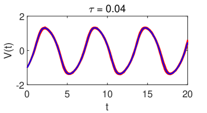
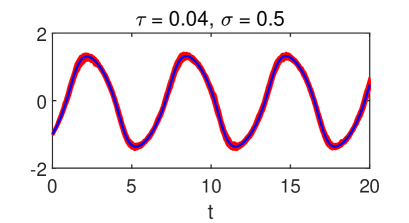
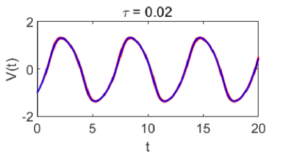
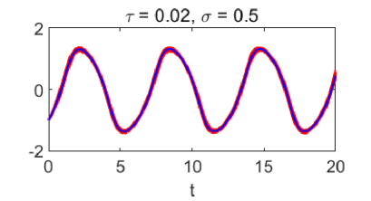
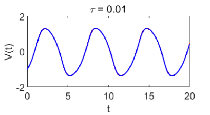
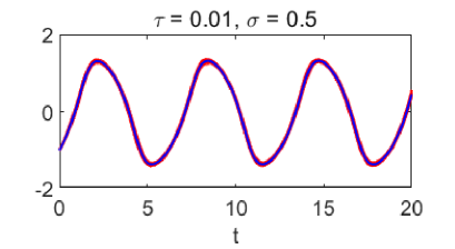
Figure 5.1. The exact trajectory of $V$ (blue) and $100$ realizations (red) computed by the probabilistic implicit Euler method with noise scale $\sigma^{*}$ (left) and fixed noise scale $\sigma=0.5$ (right).

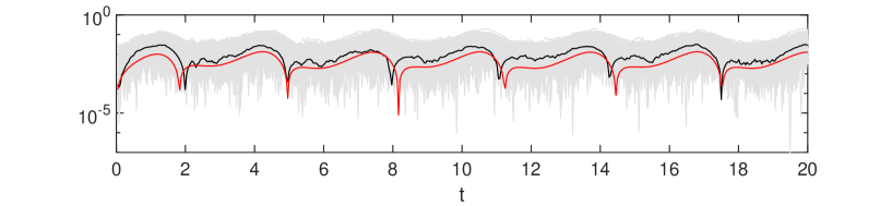
Figure 5.2. A comparison of the observed variations (gray) and their mean (black) in the calibrated probabilistic implicit Euler method using $\sigma^{*}$ and $\tau=0.04$ for the constrained FitzHugh–Nagumo model from Example 2.5. The error indicator is marked in red.

6. Conclusion

In this paper, we have introduced and analyzed a class of probabilistic time integrators of first and second order for the numerical solution of semi-linear parabolic equations with linear constraints. Such methods incorporate random perturbations, which do not affect the constraint manifold, in order to quantify the uncertainty induced by the time integration scheme. In terms of convergence, we have studied the mean square error and showed that a balanced inclusion of perturbations does not reduce the convergence order known from the deterministic setting. More precisely, the overall order equals the minimum of the (deterministic) convergence order and the order of the introduced statistical error. All results are validated through numerical experiments.

References

• [AG20] A. Abdulle and G. Garegnani. Random time step probabilistic methods for uncertainty quantification in chaotic and geometric numerical integration. Stat. Comput., 30(4):907–932, 2020.
• [AH21] R. Altmann and R. Herzog. Continuous Galerkin schemes for semiexplicit differential–algebraic equations. IMA J. of Numer. Anal., 42(3):2214–2237, 2021.
• [ALM17] R. Altmann, T. Levajković, and H. Mena. Operator differential–algebraic equations with noise arising in fluid dynamics. Monatsh. Math., 182(4):741–780, 2017.
• [Alt15] R. Altmann. Regularization and Simulation of Constrained Partial Differential Equations. Dissertation, Technische Universität Berlin, 2015.
• [AO17] R. Altmann and A. Ostermann. Splitting methods for constrained diffusion-reaction systems. Comput. Math. Appl., 74(5):962–976, 2017.
• [AZ18] R. Altmann and C. Zimmer. Runge-Kutta methods for linear semi-explicit operator differential-algebraic equations. Math. Comp., 87(309):149–174, 2018.
• [AZ20] R. Altmann and C. Zimmer. Exponential integrators for semi-linear parabolic problems with linear constraints. In T. Reis, S. Grundel, and S. Schöps, editors, Progress in Differential-Algebraic Equations II, pages 137–164. Springer International Publishing, Cham, 2020.
• [CCCG16] O. A Chkrebtii, D. A Campbell, B. Calderhead, and M. A Girolami. Bayesian solution uncertainty quantification for differential equations. Bayesian Anal., 11(4):1239–1267, 2016.
• [CGS+17] P. R. Conrad, M. Girolami, S. Särkkä, A. Stuart, and K. Zygalakis. Statistical analysis of differential equations: introducing probability measures on numerical solutions. Stat. Comput., 27(4):1065–1082, 2017.
• [EM13] E. Emmrich and V. Mehrmann. Operator differential-algebraic equations arising in fluid dynamics. Comput. Methods Appl. Math., 13(4):443–470, 2013.
• [HLR89] E. Hairer, C. Lubich, and M. Roche. The Numerical Solution of Differential-Algebraic Systems by Runge–Kutta Methods. Springer-Verlag, Berlin, 1989.
• [HO10] M. Hochbruck and A. Ostermann. Exponential integrators. Acta Numer., 19:209–286, 2010.
• [HW96] E. Hairer and G. Wanner. Solving Ordinary Differential Equations II: Stiff and Differential-Algebraic Problems. Springer-Verlag, Berlin, second edition, 1996.
• [Kai67] T. Kailath. The divergence and Bhattacharyya distance measures in signal selection. IEEE T. Commun. Techn., 15(1):52–60, 1967.
• [KM06] P. Kunkel and V. Mehrmann. Differential-Algebraic Equations: Analysis and Numerical Solution. European Mathematical Society (EMS), Zürich, 2006.
• [LB12] K. Y. Lee and T. R. Bretschneider. Separability measures of target classes for polarimetric synthetic aperture radar imagery. Asian J. Geoinform., 12(2), 2012.
• [LMT13] R. Lamour, R. März, and C. Tischendorf. Differential-Algebraic Equations: A Projector Based Analysis. Springer-Verlag, Berlin, Heidelberg, 2013.
• [LO93] C. Lubich and A. Ostermann. Runge–Kutta methods for parabolic equations and convolution quadrature. Math. Comp., 60(201):105–131, 1993.
• [LSS19] H. C. Lie, A. M Stuart, and T. J. Sullivan. Strong convergence rates of probabilistic integrators for ordinary differential equations. Stat. Comput., 29(6):1265–1283, 2019.
• [LSS22] H. C. Lie, M. Stahn, and T. J. Sullivan. Randomised one-step time integration methods for deterministic operator differential equations. Calcolo, 59(1):13, 2022.
• [Paz83] A. Pazy. Semigroups of Linear Operators and Applications to Partial Differential Equations. Springer-Verlag, New York, 1983.
• [RHCC07] J. O. Ramsay, G. Hooker, D. Campbell, and J. Cao. Parameter estimation for differential equations: A generalized smoothing approach. J. Roy. Stat. Soc. B, 69(5):741–796, 2007.
• [VR19] I. Voulis and A. Reusken. Discontinuous Galerkin time discretization methods for parabolic problems with linear constraints. J. Numer. Math., 27(3):155–182, 2019.
• [Zei90] E. Zeidler. Nonlinear Functional Analysis and its Applications IIa: Linear Monotone Operators. Springer-Verlag, New York, 1990.