Robustness of perfect transmission resonances to asymmetric perturbation

Abstract

We investigate the perfect transmission resonances (PTRs) of perturbed 1D finite periodic systems with mirror symmetric cells. The unperturbed scattering region consists of $N$ identical cells and the related transmission spectrum possesses at least $N-1$ PTRs in each pass band of the Bloch dispersion of the unit cell. On the other hand, the perturbation is breaking the periodicity and, a priori, is able to eliminate all the PTRs. We show how PTRs could still appear in the perturbed case with a suitable design of the perturbation. We also reveal a connection between two apparently independent PTRs, a connection that lies in the symmetry of the finite Kronig-Penney systems and which implies that if one PTR is preserved then another one, among the $N-1$ PTRs in a pass band, is necessarily also preserved.

I Introduction

Perfect transmission resonances (PTRs) [1], which correspond to particular frequencies where the modulus of the transmission coefficient is one, can appear in the transmission spectrum of a scattering setup [2]. PTRs are usually supported in scattering systems that posses some kind of symmetry, for instance global mirror [3, 4, 5, 6] or local [7, 8] symmetry, yet it has been found that they can occur in asymmetric systems as well [1, 9, 10]. In the framework of PTRs, one-dimensional finite periodic setups have been intensively studied [11]. When a cell is repeated $N$ times in space, then the transmission spectrum of the setup shows bands with at least $N-1$ PTRs [11, 12, 13, 14]. This result lies in the properties of the Chebychev polynomials that appear in the transfer matrix of the $N$ cells [2]. Furthermore, if the cell possesses mirror symmetry, as in the case of finite Kronig Penney models, then symmetry conditions are imposed on the scattering states corresponding to PTRs [15].

In our work we explore the impact of asymmetric perturbations on the transmission spectrum of a 1D finite periodic scattering system that is built from a mirror symmetric cell. By calculating the influence of the perturbation to the frequencies that correspond to PTRs, we determine how the design of particular asymmetric perturbations, made of a series of delta Dirac scatterers, can protect a desired PTR. Additionally, owing to the mirror symmetry of the unit cell, we prove that if the perturbing Dirac scatterers protecting a PTR (say number $n$ between 1 and $N-1$) are placed either at the centers or at the edges of the cell, then a dual PTR (number $N-n$) is protected as well.

Our work is organized as follows: In Section II, we give a brief review of scattering by a finite periodic system that is built from a mirror symmetric cell and we remind the appearance of PTRs in the transmission spectrum. In Section III, we consider a perturbation in the scattering region and we calculate the first order correction to the frequencies that correspond to the PTRs. Then, we show how we can design a perturbation that consists of Dirac scatterers and preserves a desired PTR. In Section IV, we place Dirac scatterers either at the centers or at the edges of the cells and we prove that if a PTR is preserved, then a dual PTR is preserved as well. In Section V, we discuss the asymmetry of the scattering states corresponding to perturbed PTR and in Section VI we explore the impact of the perturbation strength to PTRs. Finally in Section VII we summarize our findings.

II Reminder on scattering by a periodic system with mirror symmetric cells

We begin by reminding some basic properties of the wave scattering in one dimension by a setup that is finite periodic and mirror symmetric. We consider waves satisfying the stationary Schrödinger equation

$$\psi^{\prime\prime}+\left[k^{2}-\mathcal{V}_{0}(x)\right]\psi=0$$ (1)

where prime denotes differentiation with respect to space coordinate $x$, $\psi$ is the wave function, $k$ is the frequency and $\mathcal{V}_{0}(x)$ is the potential which is nonzero only for $x\in[-D/2,D/2]$.

The potential $\mathcal{V}_{0}(x)$ is assumed to be real and finite periodic as described in Fig. 1(a). For reasons that will appear later, we choose a mirror symmetric unit cell. Such a potential $\mathcal{V}_{0}$ is written in the following form

$$\mathcal{V}_{0}(x)=\sum_{n=1}^{N}{V}_{0}\left(x+\frac{d}{2}(N+1)-nd\right),$$ (2)

where $V_{0}(x)=V_{0}(-x)$ is real and zero outside the region $[-d/2,d/2]$.

The transfer matrix of the building cell gets the form [16]

$$\mathbf{M}=\begin{pmatrix}1/t^{*}&&r/t\\ -r/t&&1/t\end{pmatrix}.$$ (3)

where $t$ ($r$) is the transmission (reflection) amplitude and since $V_{0}$ is real, $T+R=1$ where $T=|t|^{2}$ ($R=|r|^{2}$) is the transmission (reflection) coefficient of the cell. The transfer matrix of the periodic setup with $N$ cells, $\mathbf{M}^{N}$, is given by

$$\mathbf{M}^{N}=\begin{pmatrix}1/t_{N}^{*}&&r_{N}/t_{N}\\ -r_{N}/t_{N}&&1/t_{N}\end{pmatrix}.$$ (4)

where $t_{N}$ ($r_{N}$) is the transmission (reflection) amplitude of the $N$ cells. Similarly to the single cell case, $T_{N}+R_{N}=1$ where $T_{N}=|t_{N}|^{2}$ and $R_{N}=|r_{N}|^{2}$ are now the transmission and reflection coefficients of the $N$ cells. Owing to the Chebychev identity [2], one can write $\mathbf{M}^{N}$ as

$$\mathbf{M}^{N}=\begin{pmatrix}\dfrac{1}{t^{*}}\dfrac{\sin(N\phi)}{\sin(\phi)}-\dfrac{\sin\left((N-1)\phi\right)}{\sin(\phi)}&&\dfrac{r}{t}\dfrac{\sin(N\phi)}{\sin(\phi)}\\ -\dfrac{r}{t}\dfrac{\sin(N\phi)}{\sin(\phi)}&&\dfrac{1}{t}\dfrac{\sin(N\phi)}{\sin(\phi)}-\dfrac{\sin\left((N-1)\phi\right)}{\sin(\phi)}\end{pmatrix}$$ (5)

where $\phi=\dfrac{1}{2}\text{Tr}[\mathbf{M}]$ is the Bloch phase of the unit cell.

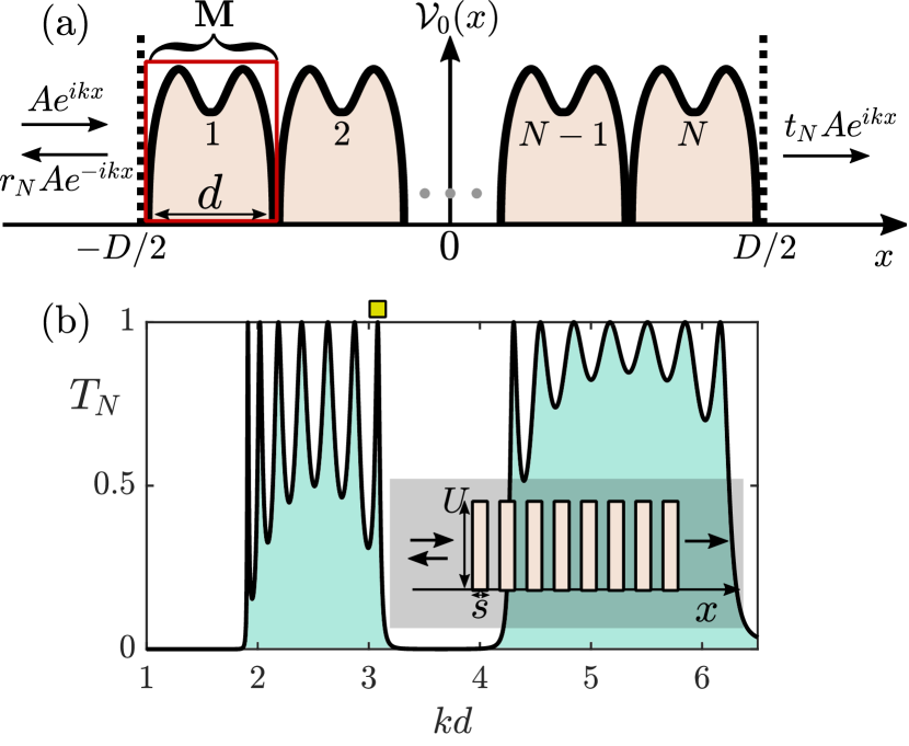
Figure 1: (a) Schematic description of the scattering of a wave with amplitude $A$ and frequency $k$ by a finite periodic setup that consists of $N$ mirror symmetric cells. The length of each cell is $d$ and of the whole setup is $D$, where $D=Nd$. Also, $t_{N}$ ($r_{n}$) is the transmission (reflection) amplitude. (b) Transmission spectrum $T_{N}(k)=|t_{N}(k)|^{2}$ of a finite periodic scattering setup that consists of 8 rectangular barriers (the scattering setup is shown in the inset). The length of each barrier is $s=d/6$ and therefore the free space between two neighboring barriers has length $5d/6$ (notice that the setup in the inset is not representing such distances). The heights of the barriers, $U=\displaystyle\max_{x}V_{0}(x)$, are set at $\sqrt{U}\approx 5.196/d$.

Since we are focusing on PTRs in finite periodic setups a useful expression for the transmission coefficient of the $N$ cells is [11, 12, 13, 2]

$$T_{N}=\displaystyle{\dfrac{1}{1+\left(\dfrac{1}{|t|^{2}}-1\right)\dfrac{\sin^{2}(N\phi)}{\sin^{2}(\phi)}}}.$$ (6)

In Eq. (6) PTRs, i.e. $T_{N}=1$, are obtained when $\phi_{n}=n\pi/N+\mod(2\pi)$ with $n=1,2,...,N-1$ since $\sin(N\phi_{n})=0$. Additional PTRs appear as well whenever $T=1$. In Fig. 1(b) is displayed the transmission spectrum $T_{N}(k)$ of a periodic setup with 8 rectangular barriers (the setup is shown in the inset). The transmission spectrum shows a band-like structure with $N-1=7$ PTRs in each band since there is no $k$ for which $T(k)=1$ in this frequency range.

As a remark we note that PTRs correspond to real eigenvalues of the reflectionless mode eigenproblem [17, 18], given by solution of Eq. (1) with boundary conditions

$$\left.\dfrac{d\psi(x)}{dx}\right|_{x=\pm D/2}-ik\psi(\pm D/2)=0.$$ (7)

One property of this reflectionless eigenvalue problem is that when the potential $\mathcal{V}_{0}(x)$ is mirror symmetric $\mathcal{V}_{0}(x)=\mathcal{V}_{0}(-x)$, this eigenvalue problem becomes $\mathcal{PT}$-symmetric. It means that perturbing the symmetric $\mathcal{V}_{0}(x)$ and keeping the mirror symmetry, PTRs are protected (but are displaced in the transmission spectrum) as long as they do not coalesce at the exceptional points of the $\mathcal{PT}$-symmetric reflectionless eigenvalue problem. In contrast, breaking the mirror symmetry of the potential no PTR-protection is anticipated and we are going to inspect how non-mirror symmetric perturbations are capable to asymptotically keep desired PTRs.

III Perturbing the potential

We consider that $\mathcal{V}_{0}(x)$ is perturbed and the scattering region is described by the potential

$$\mathcal{V}(x)=\mathcal{V}_{0}(x)+\epsilon\mathcal{V}_{1}(x),$$ (8)

where $\mathcal{V}_{1}(x)$ is the perturbation and $\epsilon$ is a small parameter, i.e. $\epsilon\ll 1$. As for $\mathcal{V}_{0}(x)$, we let the perturbing potential $\mathcal{V}_{1}(x)$ to be nonzero only inside the region $[-D/2,D/2]$.

III.1 First order correction

We aim to find the variation at the frequencies that correspond to PTRs. We denote the unperturbed frequencies corresponding to $\mathcal{V}_{0}$ as $k_{0,n}$ (where the index $n$ is the number of the PTR in one pass band, $n=1,2,...,N-1$). Following the asymptotic perturbation approach of reflectionless modes in ref. [19], we write the perturbed frequencies as

$$k_{n}=k_{0,n}+\epsilon k_{1,n}+\ldots$$ (9)

and by applying the classical solvability condition we find that the first order correction $k_{1,n}$ is given by (see Appendix A for the details)

$$k_{1,n}=\dfrac{\int_{-D/2}^{D/2}\mathcal{V}_{1}\psi^{2}_{0,n}dx}{i[\psi_{0,n}^{2}(D/2)-\psi_{0,n}^{2}(-D/2)]+2k_{0,n}\int_{-D/2}^{D/2}\psi^{2}_{0,n}dx}.$$ (10)

In the last expression $\psi_{0,n}$ is the PTR wave function for frequency $k_{0,n}$. To asymptotically keep a PTR at order $O(\epsilon)$ it is sufficient to look for zero imaginary part of $k_{1,n}$. Then, the real part of $k_{1,n}$ shows how this PTR is shifted in the transmission spectrum.

From Eq. (10) it appears that we just have to deal with overlap integrals involving $\mathcal{V}_{1}$ and $\psi_{0,n}$, where the symmetry of $\psi_{0,n}$ plays an important role. In fact, for a mirror symmetric potential $\mathcal{V}_{0}$ as the one illustrated in Fig. 1(a), great simplification can be obtained. Indeed, by the suitable phase transformation described below, the real and imaginary parts of $\psi_{0,n}$ become symmetric and antisymmetric around $x=0$ respectively (see for example Fig. 2). In that case, the denominator in Eq. (10) is real and therefore the imaginary part of $k_{1,n}$ is given by

$$\text{Im}[k_{1,n}]=\mathcal{C}\int_{-D/2}^{D/2}\mathcal{V}_{1}\text{Re}[\psi_{0,n}]\text{Im}[\psi_{0,n}]dx$$ (11)

with $\mathcal{C}$ real. Considering scattering from the left side of the potential $\mathcal{V}_{0}(x)$ [see Fig. 1(a)], the phase that symmetrizes the wave function is obtained by setting the amplitude $A$ of the incoming wave equal to

$$A=\begin{cases}e^{ik_{0,n}D/2},~{}~{}~{}~{}~{}~{}~{}~{}~{}\text{for even}~{}n\\ e^{ik_{0,n}D/2-i\pi/2},~{}~{}\text{for odd}~{}n\end{cases}.$$ (12)

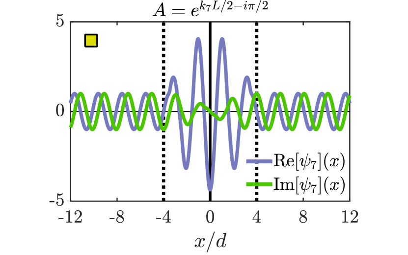
Figure 2: Real and imaginary parts of the wave function $\psi_{7}(x)$ for frequency $k_{7}$ (corresponding to the PTR number $n=7$) of the unperturbed setup that is shown in Fig. 1(b) (indicated with a yellow square). The amplitude of the incoming wave is set at $A=e^{ik_{7}H/2-\pi/2}$ [see Eq. (12)].

As mentioned before, in mirror symmetric perturbations the PTRs are kept. It means that if the perturbing potential $\mathcal{V}_{1}$ is an even function with respect to $x=0$ (mirror symmetric perturbation) then from Eq. (11) we get $\text{Im}[k_{1,n}]=0$ for all $n$, since $\text{Re}[\psi_{0,n}]\text{Im}[\psi_{0,n}]$ is odd for all $n$. In Fig. 3 we present such an example. In the following we show how we can design an asymmetric perturbing potential $\mathcal{V}_{1}$ that preserves PTRs.

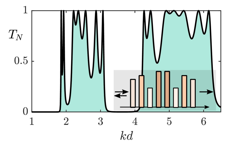
Figure 3: Mirror symmetric perturbation ($\epsilon=0.1$). Shown is the transmission spectrum of the scattering setup that is displayed in the inset. This scattering setup is derived by perturbing in a mirror symmetric way the barriers of the setup shown in Fig. 1(b). The lengths of the barriers and the distances between two neighboring barriers are the same as in Fig. 1(b). The perturbations $U_{i}$ in each barrier $i=1,2,...,8$ are set at $U_{1}=U_{8}=-27/d^{2}$, $U_{2}=U_{7}=0$, $U_{3}=U_{6}=-72/d^{2}$ and ${U}_{4}={U}_{5}=27/d^{2}$.

III.2 Preserving one PTR with asymmetric perturbation

Choosing $\mathcal{V}_{1}$ to be a sum of Dirac scatterers

$$\mathcal{V}_{1}=\sum_{m=1}^{M}c_{m}\delta(x-x_{m})$$ (13)

where $c_{m}$ are the strengths of the scatterers and $x_{m}\in[-D/2,D/2]$ are their positions, Eq. (11) takes the simple form

$$\text{Im}[k_{1,n}]=\mathcal{C}\sum_{m=1}^{M}c_{m}\text{Re}[\psi_{0,n}(x_{m})]\text{Im}[\psi_{0,n}(x_{m})].$$ (14)

Based on this form, we can achieve $\text{Im}[k_{1,n}]=0$ for a specific PTR number $n$ with asymmetric $\mathcal{V}_{1}$. Actually, since $\psi_{0,n}(x)$ is given, $\text{Im}[k_{1,n}]=0$ takes the form of one equation with $M$ unknowns ($c_{m}$, $m=1,...,M$)

$$\sum_{m=1}^{M}c_{m}\text{Re}[\psi_{0,n}(x_{m})]\text{Im}[\psi_{0,n}(x_{m})]=0.$$ (15)

To comply with this equation, the minimal number of perturbing Dirac scatterers is generically $M=2$, resulting in a simple proportionality between $c_{1}$ and $c_{2}$ (accidental location where $\text{Re}[\psi_{0}]\text{Im}[\psi_{0}]=0$ would allow $M=1$). As an illustration, consider the scattering by the potential shown in Fig. 4(a). With $N=8$, it displays how to keep PTR $n=7$ with 2 Dirac scatterers. Note that only the PTR $n=7$ is kept, while all the 6 other are lost.

We remark that we might generalize this procedure by increasing the number of perturbing Dirac scatterers allowing to preserve larger number of PTRs. In principle, to keep $q$ PTRs we would need $q+1$ Dirac scatterers. In the sequel, we show that due to the mirror symmetry of the unit cell, 2 PTRs can be preserved with only 2 Dirac perturbations when properly located.

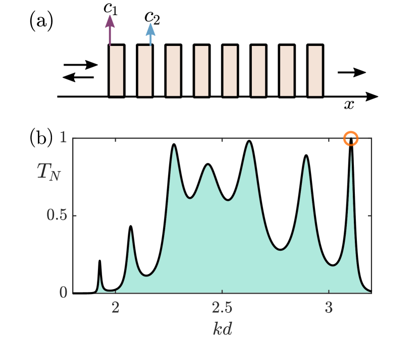
Figure 4: Asymmetric perturbation preserving one PTR ($\epsilon=0.1$). (a) Schematic description of the wave scattering by a setup that consists of eight rectangular barriers (unperturbed potential $\mathcal{V}_{0}$) and two Dirac scatterers (perturbing potential $\mathcal{V}_{1}$). The heights of the barriers $U$, their lengths $s$ and the free space between two neighboring barriers are the same as in Fig. 1(b). The first (second) Dirac scatterer is placed at a distance of $0.1s$ ($0.95s$) from the left edge of the first (second) barrier. The strength of the first Dirac scatterer is set at $c_{1}=4.8/d$ and the strength of the second Dirac scatterer is found from Eq. (15), so that the PTR number $n=7$ of the unperturbed setup is preserved after the addition of the two scatterers. (b) Transmission spectrum of the setup that is shown in (a). Only the PTR number $n=7$ of the unperturbed setup is preserved (indicated with a circle).

IV Exploiting the mirror symmetry to keep PTRs in pairs

When the unperturbed unit cell is mirror symmetric, particular properties come out for perturbing Dirac scatterers, located either all at the centers or all at the edges of the cells of $\mathcal{V}_{0}$.

IV.1 Dirac scatterers at the centers of the cells

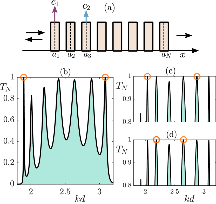
Figure 5: PTRs preserved in pairs: Dirac scatterers located at the centers of the cells ($\epsilon=0.1$). (a) Schematic description of the wave scattering by a setup that consists of 8 rectangular barriers ($\mathcal{V}_{0}$) and 2 Dirac scatterers ($\mathcal{V}_{1}$) of strengths $c_{1,2}$ that are placed at the centers of the first and third cells. Again, the lengths of the barriers $s$, the free space between two neighboring barriers and their heights $U$ are the same as in Fig. 1(b). (b)-(d) Transmission spectrum of the setup that is shown in (a). Specifically: (b) The strength $c_{1}$ is set at $c_{1}=12/d$. The strength $c_{2}$ is designed through Eq. (15) so that the PTR number $n=1$ of $\mathcal{V}_{0}$ is preserved after the addition of the two scatterers. The PTR number $n=7$ is also preserved. (c) We set $c_{1}=4.5/d$ and we calculate the strength $c_{2}$ so that PTR number $n=2$ of $\mathcal{V}_{0}$ is preserved. The PTR number $n=6$ is preserved as well. (d) We set $c_{1}=2.4/d$ and we design $c_{2}$ so that the PTR number $n=3$ of $\mathcal{V}_{0}$ is preserved. Then the PTR number $n=5$ is also preserved.

Let us start with the presentation of an example: an incident wave is scattered by the potential shown in Fig. 5(a). This potential consists of $N=8$ rectangular barriers ($\mathcal{V}_{0}$) and $M=2$ Dirac scatterers ($\mathcal{V}_{1}$) that are placed at the centers of the first and third barriers. In Fig. 5(b)-(d) we illustrate the transmission spectrum initially designed to protect one PTR (either PTR number $n=1$, $n=2$ or $n=3$).

In Fig. 5(b) we design the strengths $c_{1}$ and $c_{2}$ [from Eq. (15)] so that the PTR $n=1$ is preserved. Surprisingly, it appears that apart from the PTR $n=1$, the PTR $n=7$ is preserved as well. In Fig. 5(c) and (d) the same kind of behavior is observed: when designing perturbation protecting PTR number $n$, the PTR number $N-n$ is also protected.

In fact it can be proven that if a periodic potential with mirror symmetric cells (not necessarily rectangular cells) is perturbed by Dirac scatterers placed at the centers of the cells, then the PTRs are preserved in pairs. More specifically, we show that

$$\text{Im}[k_{1,n}]=0\Rightarrow\text{Im}[k_{1,N-n}]=0$$ (16)

for perturbations at the centers of the cells. A sketch of the proof is as follows:

• In appendix B we prove that for the centers $a_{p}$ of the cells ($p=1,2,...,N$)

  $$\text{Re}[\psi_{0,n}(a_{p})]\text{Im}[\psi_{0,n}(a_{p})]=f(\phi_{n})g(p,\phi_{n})$$ (17)

  where

  $$g(p,\phi_{n})=\sin^{2}\left[(N-p)\phi_{n}\right]-\sin^{2}\left[(p-1)\phi_{n}\right]$$ (18)

  and

  $$\phi_{n}=\dfrac{n\pi}{N}$$ (19)

  is the Bloch phase of the $n^{th}$ PTR.
  

• Equations (18) and (19) suggest that under the interchange $n\rightarrow N-n$:

  $$\phi_{N-n}=\pi-\phi_{n}\Rightarrow g(p,\phi_{n})=g(p,\phi_{N-n}).$$ (20)

  Using Eq. (17) and Eq. (20) we can show that if Eq. (15) holds for $n$, it holds for $N-n$ as well, implying property (16).

More details can be found in Appendix B.

IV.2 Dirac scatterers at the edges of the cells

In the previous subsection we considered the case of Dirac scatterers located at the centers of cells. Here the Dirac scatterers are placed at the edges of cells. The results of the previous subsection still apply, while an additional property is revealed.

In line with our previous approach, we begin by illustrating an example. We consider the wave scattering by the potential shown in Fig. 6(a). As previously, the unperturbed potential $\mathcal{V}_{0}$ consists of $N=8$ rectangular barriers. We place $M=2$ Dirac scatterers of strengths $c_{1,2}$ at the right edges of the first and second cells. Without surprise, by choosing $c_{1,2}$ according to Eq. (15) the PTRs number $n$ and $N-n$ are simultaneously preserved, as shown in the transmission spectra in Fig. 6(b)-(c) [20]. This property (also true for the setup of subsection A) appears for any $N$ even or odd.

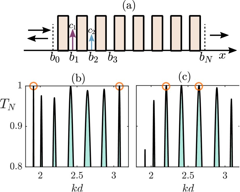
Figure 6: Protection of PTRs when Dirac scatterers are placed at the edges of the cells ($\epsilon=0.1$). (a) Schematic description of the scattering of a wave by a setup that consists of 8 rectangular barriers ($\mathcal{V}_{0}$) and 2 Dirac scatterers ($\mathcal{V}_{1}$) of strengths $c_{1,2}$ that are placed at the right edges of the first and second cells. The heights $U$ of the barriers, their lengths $s$, the free space between two neighboring barriers are as in Fig. 1(b). (b)-(c) Transmission spectrum of the setup that is shown in (a): (b) We set the strength $c_{1}$ of the first Dirac scatterer equal to $c_{1}=1.8/d$ and we calculate $c_{2}$ from Eq. (15) so that the PTR $n=1$ is preserved. We find that the PTR number $n=7$ is also preserved. (c) We set $c_{1}=1.8/d$ and we calculate $c_{3}$ again from Eq. (15) so that the PTR number $n=3$ is preserved. We find that the PTR number $n=5$ is preserved as well.

What is surprising is the following: if the number of cells $N$ is even and the Dirac scatterers are placed at the $b_{p}$’s with the same parity – $p$ can only take the values $p=1,3,5,...$ (or $p=0,2,4,...$) – so that the PTR number $n$ is protected, then not only the PTR number $N-n$ but also the PTRs number $N/2\pm n$ get protected. To illustrate this, we consider the scattering by the setup shown in Fig. 7(a), where the 2 Dirac scatterers are placed at the edges $b_{1}$ and $b_{3}$. Shown in Fig. 7(b) and (c) are the transmission spectra for 2 choices $c_{1,2}$ where the perturbation is designed to protect the PTR $n=1$ and $n=2$ respectively. Notice that in panel (b), by protecting one PTR, we actually protect three more according to the previous discussion.

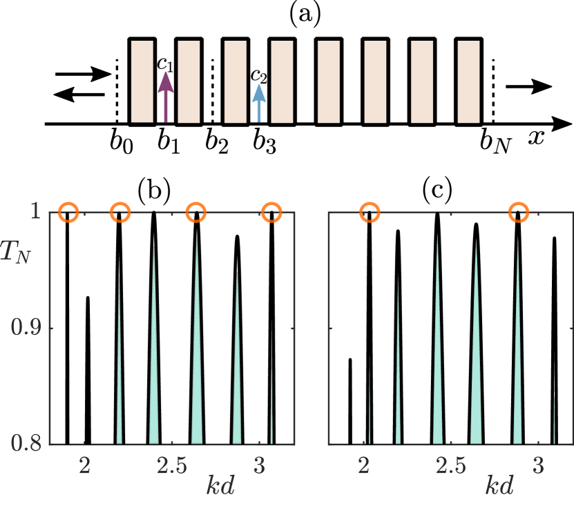
Figure 7: Same as in Fig. 6 but now the 2 Dirac scatterers are placed at the edges $b_{1}$ and $b_{3}$. (b)-(c) We set $c_{1}=1.5/d$ and we calculate $c_{2}$ from Eq. (15). The PTRs in (b) are protected in multiplets.

We now show analytically all the aforementioned connections between PTRs. That is, we show that when the Dirac scatterers are placed at the edges $b_{p}$ of cells then property (16) still holds, namely $\text{Im}[k_{1,n}]=0\Rightarrow\text{Im}[k_{1,N-n}]=0$ . Moreover, if the scatterers are placed at the $b_{p}$’s with the same parity, i.e. $p=1,3,5$ (or $p=0,2,4,...$), the additional property

$$\text{Im}[k_{1,n}]=0\Rightarrow\text{Im}[k_{1,N/2\pm n}]=0$$ (21)

also holds. As we did in the previous subsection, we give an outline of the steps of the proof and details can be found in Appendix C:

• There we show that at the edges $b_{p}$ of the cells ($p=0,1,2,...,N$) the following relation holds

  $$\text{Re}[\psi_{0,n}(b_{p})]\text{Im}[\psi_{0,n}(b_{p})]=\tilde{f}(\phi_{n})\tilde{g}(p,\phi_{n})$$ (22)

  where

  $$\tilde{g}(p,\phi_{n})=\sin(2p\phi_{n}).$$ (23)

  and $\phi_{n}$ is the Bloch phase of the $n^{th}$ PTR [see Eq. (19)].
  

• Under the interchange $n\rightarrow N-n$, from Eq. (23) we get that

  $$\tilde{g}(p,\phi_{n})=\tilde{g}(p,\phi_{N-n}).$$ (24)

  We can prove Eq. (16), using Eq. (15), (22) and (24) as we did in the previous subsection.
  

• Under the interchange $n\rightarrow N/2\pm n$, from Eq. (23) we obtain that

  $$\tilde{g}(p,\phi_{N/2\pm n})=(-1)^{p}\tilde{g}(p,\phi_{n}).$$ (25)

  Notice that if $N$ is even and $p$ is only odd or only even, then we can prove property (21) using Eq. (15), (22) and (25).

V Asymmetry of the wave field

Up to this point, we have studied the variation of the frequencies $k_{0,n}$ under perturbations [recall Eq. (9)]. We now focus on the perturbed wave field

$$\psi_{n}=\psi_{0,n}+\epsilon\psi_{1,n}+\ldots~{}.$$ (26)

We will explore whether an asymmetric perturbation protecting the PTR number $n$, breaks the mirror symmetry of $|\psi_{0,n}|$, thus inducing an asymmetric wave field $\psi_{n}$. This is interesting because it enables the appearance of non-reciprocal scattering when appropriate non-linearity is added, leading to an asymmetric transmission [21] and even to all-optical-diodes [1, 22, 23, 24].

To this end, we use the asymmetric setup shown in Fig. 5(a) with Dirac scatterers designed to protect the PTR $n=1$ and we consider scattering either from the left or from the right side of this perturbed setup. In Fig. 8 we show the corresponding norms of the exact fields $\psi_{n}^{L}$ and $\psi_{n}^{R}$ (in the presence of the perturbation for $n=1$) with dashed and dotted lines respectively. With the arrows we indicate the direction of the incident waves. For comparison, we also show with a solid line the unperturbed $|\psi_{0,n}|$ for $n=1$.

Notice that the fields $\psi_{n}^{L}$ and $\psi_{n}^{R}$ are asymmetric and close to resonance (transmission coefficient $T_{N}\approx 0.9$). Moreover, we note that the asymmetry of $\psi_{n}$ grows as the value of the perturbation parameter $\epsilon$ increases (a large value of $\epsilon$ suggests the perturbed setup is strongly asymmetric). Yet for large $\epsilon$ it is expected that the transmission for frequency $k_{n}$ [recall Eq. (9)] is not close to 1, meaning that the wave field $\psi_{n}$ is not at resonance. Therefore, a natural step is to investigate the influence of $\epsilon$ on PTRs.

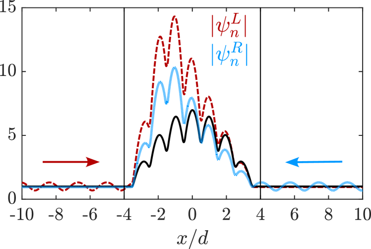
Figure 8: The scattering setup is the one shown in Fig. 5(a) for $\epsilon=0.225$. The red dashed (blue dotted) line denotes the wave field norm, for frequency $k_{1}\approx 1.86696/d$ (corresponding to the first peak of the frequency spectrum), when scattering from the left (right) side of the setup is considered. The black solid line represents $|\psi_{0,n}|$ for $n=1$.

VI Fate of PTRS under increasing perturbation strength

Before closing, we examine how the perturbation strength $\epsilon$ affects protected- and unprotected-PTRs by perturbations. Firstly, we remind that to lose a PTR under mirror symmetric perturbations the eigenvalues of the $\mathcal{PT}$-symmetric problem given in Eq. (7) must merge (recall the discussion at the end of Section II). We show in Fig. 9 with the solid line such an example for the range of $\epsilon$ values for which the problem remains $\mathcal{PT}$-symmetric. Thus, the transmission remains equal to 1 for these values of $\epsilon$.

Secondly, we show in Fig. 9 with a dashed line the transmission of a protected PTR by an asymmetric perturbation. This line drops as $1-|\epsilon|^{4}$ since the reflection coefficient for PTR-protected perturbation increases as $r\sim\epsilon^{2}$ as predicted.

Finally, with the dotted line, we present the transmission of an unprotected PTR under the same asymmetric perturbation as in the latter case. Here, the line drops as $1-|\epsilon|^{2}$ since the reflection coefficient $r$ is of order $\epsilon$.

VII Concluding remarks

In this paper, starting from a finite periodic setup with $N$ mirror symmetric cells, we have investigated how the scattering is influenced by asymmetric perturbation. More specifically, using a perturbation consisting of a sum of Dirac scatterers, our goal was to preserve specific PTRs among the $N-1$ PTRs of the unperturbed system. First, we have demonstrated that using $q+1$ Dirac scatterers it is possible to keep $q$ PTRs of the unperturbed system. Then, the mirror symmetry of the unit cell was shown to have an important role manifested through the preservation of additional PTRs; i.e. PTRs have to be preserved in pairs when the perturbing Dirac scatterers are located at symmetry points of the unit cell. The obtained PTRs with asymmetric scatterers are accompanied by asymmetric scattering states and open the possibility to non-reciprocal scattering when appropriate non-linearity is added.

Similarly to the case of finite periodic real potentials, it is known that finite periodic complex potentials that are $\mathcal{PT}$-symmetric, support at least $N-1$ PTRs due to periodicity [25]. Therefore, the possible generalization of our results to a $\mathcal{PT}$-symmetric potential and the study of the impact of a $\mathcal{PT}$-symmetry breaking point could certainly be of interest. Finally, the construction of a perturbation that preserves PTRs but it is not comprised with Dirac scatterers could be of additional interest since it would open more possibilities for experimental realizations.

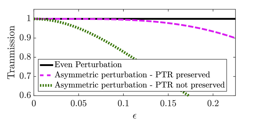
Figure 9: The solid black line denotes the transmission of PTR number $n=1$ shown in Fig. 3. The dashed magenta (dotted green) denotes the transmission of PTR number $n=1$ ($n=2$) shown in Fig. 5(a).

Appendix A Perturbative expression

The wave function $\psi_{n}(x)$ and the frequency $k_{n}$ corresponding to the PTR number $n$ of the potential $\mathcal{V}(x)$, satisfy the Schrödinger equation

$$\dfrac{d^{2}\psi_{n}}{dx^{2}}+\left(k_{n}^{2}-\mathcal{V}(x)\right)\psi_{n}=0$$ (27)

and the boundary conditions

$$\left.\dfrac{d\psi_{n}(x)}{dx}\right|_{x=\pm D/2}=ik_{n}\psi_{n}(\pm D/2)$$ (28)

where the region $[-D/2,D/2]$ is the scattering area.

We write the potential $\mathcal{V}(x)$ in the perturbed form (Eq. (8))

$$\mathcal{V}(x)=\mathcal{V}_{0}(x)+\epsilon\mathcal{V}_{1}(x)$$ (29)

and the wave function function $\psi_{n}$ and frequency $k_{n}$ as

$$\psi_{n}=\psi_{0,n}+\epsilon\psi_{1,n}+\ldots$$ (30)

$$k_{n}=k_{0,n}+\epsilon k_{1,n}+\ldots$$ (31)

that is Eq. (26) and Eq. (9) respectively. By plugging Eq. (29)-(31) into Eq. (27)-(28) and collecting in powers of $\epsilon$, we find that $\psi_{0,n}$ and $k_{0,n}$ satisfy the zeroth order problem (Eq. (27)-(28)).

After a few manipulations, we find that the correction $\psi_{1,n}$ satisfies the equation

$$\dfrac{d^{2}\psi_{1,n}(x)}{dx^{2}}+\left(k_{0,n}^{2}-\mathcal{V}_{0}\right)\psi_{1,n}=-\left(2k_{0,n}k_{1,n}-\mathcal{V}_{1}\right)\psi_{0,n}$$ (32)

and the boundary conditions

$$\left.\dfrac{d\psi_{1,n}(x)}{dx}\right|_{x=\pm D/2}-ik_{0,n}\psi_{1,n}(\pm D/2)=ik_{1,n}\psi_{0,n}(\pm D/2)~{}.$$ (33)

By multiplying Eq. (32) with $\psi_{0,n}$, integrating in the scattering region $[-D/2,D/2]$, and using the equations that $\psi_{0,n}$ and $\psi_{1,n}$ satisfy, we arrive at Eq. (10) of the main text (expression for $k_{1,n}$).

Appendix B Centers of the cells - Proof

We give here the steps needed for the derivation of Eq. (17) and (18). As we stated in the main text, these two equations hold for the centers of the cells, $a_{p}$ with $p=1,...,N$, and for the case of PTRs (denoted throughout this work with the index $n$).

We begin by reminding that the cells were considered to possess mirror symmetry. Due to the latter symmetry, the transfer matrix $\mathbf{M}$ of each unit cell [see Eq. (3)], is decomposed around the axis of symmetry as $\mathbf{M}=\mathbf{M}_{2}\mathbf{M}_{1}$ where

$$\mathbf{M}_{2}^{-1}=\mathbf{P}\mathbf{M}_{1}\mathbf{P}$$ (34)

and

$$\mathbf{P}=\begin{pmatrix}0&&1\\ 1&&0\end{pmatrix}$$ (35)

is the parity operator. Therefore, by setting [13]

$$\mathbf{M}_{1}=\begin{pmatrix}\alpha&&\beta\\ \beta^{*}&&\alpha^{*}\end{pmatrix}$$ (36)

then from Eq. (34)-(36) it follows that

$$\mathbf{M}_{2}^{-1}=\begin{pmatrix}\alpha^{*}&&\beta^{*}\\ \beta&&\alpha\end{pmatrix}.$$ (37)

As a next step, we define the vector $\bm{\chi}$ containing the right- and left-going waves at each point along the $x$-axis. For scattering from the left side of the potential and for a frequency of the incident wave corresponding to the PTR $n$, the following relation holds

$$\bm{\chi}_{n}(-D/2)=\begin{pmatrix}1\\ 0\end{pmatrix}$$ (38)

where $x=-D/2$ is the left edge of the scattering setup, see Fig. 1(a). The wave function $\psi$ is the sum of the right- and left-going waves (the sum of the two components of the vector $\bm{\chi}$), and therefore we get that

$$\psi_{n}(-D/2)=1.$$ (39)

Next, we calculate the vector $\bm{\chi}_{n}$ at the right edge of the scattering setup, namely at the point $x=D/2$. To achieve this, we use the Chebychev identity which states that if the transfer matrix $\mathbf{M}$ is written in the form

$$\mathbf{M}=\begin{pmatrix}m_{11}&&m_{12}\\ m_{21}&&m_{22}\end{pmatrix}$$ (40)

then the matrix $\mathbf{M}^{N}$ is given by

$$\footnotesize\mathbf{M}^{N}=\begin{pmatrix}m_{11}U_{N-1}-U_{N-2}&&m_{12}U_{N-1}\\ m_{12}U_{N-1}&&m_{22}U_{N-1}-U_{N-2}\end{pmatrix}$$ (41)

where

$$U_{N}=\dfrac{\sin((N+1)\phi)}{\sin(\phi)}.$$ (42)

and $\phi$ is the Bloch phase. For the case of a PTR, the Bloch phase is equal to $\phi_{n}=n\pi/N$ (recall Eq. (19)) and therefore we get that

$$\bm{\chi}_{n}(D/2)=\begin{pmatrix}(-1)^{n}\\ 0\end{pmatrix}$$ (43)

meaning that

$$\psi_{n}(D/2)=(-1)^{n}.$$ (44)

Subsequently, we calculate the wave function $\psi_{n}$ at the point $a_{1}$ ($a_{N}$), namely at the center of the first (last) cell. Using Eq. (36) and (38), we get that

$$\bm{\chi}_{n}(a_{1})=\mathbf{M}_{1}\bm{\chi}(-D/2)=\begin{pmatrix}\alpha\\ \beta^{*}\end{pmatrix},$$ (45)

and therefore the wave function $\psi_{n}$ at the center of the first cell is given by

$$\psi_{n}(a_{1})=\alpha+\beta^{*}.$$ (46)

Similarly, at the point $a_{N}$:

$$\bm{\chi}_{n}(a_{N})=\mathbf{M}_{2}^{-1}\bm{\chi}_{n}(D/2)=\begin{pmatrix}(-1)^{n}\alpha^{*}\\ (-1)^{n}\beta\end{pmatrix},$$ (47)

and as a result

$$\psi(a_{N})=(-1)^{n}(\alpha^{*}+\beta).$$ (48)

We now proceed to calculate the wave function at the center of each cell ($a_{p}$ with $p=1,...,N$): to accomplish this, first we define the transfer matrix ${\mathbf{\tilde{M}}}=\mathbf{M}_{1}\mathbf{M}_{2}$. Notice that $\mathbf{\tilde{M}}$ differs from the transfer matrix $\mathbf{M}$ of a cell, which as we noted before is equal to $\mathbf{M}=\mathbf{M}_{2}\mathbf{M}_{1}$. The two eigenvectors $\bm{v}_{q}$ and $\bm{v}_{-q}$ of ${\mathbf{\tilde{M}}}$ can be written in the following form (since $\det({\mathbf{\tilde{M}}})=1$)

$$\bm{v}_{q}=\dfrac{1}{\sqrt{1+|\kappa|^{2}}}\begin{pmatrix}1\\ \kappa\end{pmatrix}~{}~{}\text{and}~{}~{}\bm{v}_{-q}=\dfrac{1}{\sqrt{1+|\kappa|^{2}}}\begin{pmatrix}\kappa^{*}\\ 1\end{pmatrix},$$ (49)

and $\kappa=\kappa^{*}$ due to the mirror symmetry of the cell; for non-mirror symmetric cell $\kappa\in\mathbb{C}$. We express now the vector $\bm{\chi}_{n}(a_{1})$ in the basis formed by $\bm{v}_{q}$ and $\bm{v}_{-q}$,

$$\bm{\chi}_{n}(a_{1})=A\bm{v}_{q}+B\bm{v}_{-q},$$ (50)

where the coefficients $A$ and $B$ will be determined in the following step by the conditions given in Eq. (46) and (48); the wave function at the point $a_{1}$ is written in the form

$$\psi(a_{1})=Az+Bz^{*}$$ (51)

where $z=\dfrac{1+\kappa}{\sqrt{1+|\kappa|^{2}}}$.

By acting on the vector $\bm{\chi}_{n}(a_{1})$ given in Eq. (50) with the transfer matrix ${\mathbf{\tilde{M}}}^{p-1}$, we compute the vector $\bm{\chi}_{n}(a_{p})$ and then we get the wave function at the center $a_{p}$ of a cell:

$$\bm{\chi}_{n}(a_{p})=Ae^{i(p-1)\phi_{n}}\bm{v}_{q}+Be^{-i(p-1)\phi_{n}}\bm{v}_{-q}$$ (52)

and therefore

$$\psi(a_{p})=Ae^{i(p-1)\phi_{n}}z+Be^{-i(p-1)\phi_{n}}z^{*}.$$ (53)

The two coefficients $A$ and $B$ are found by using Eq. (46) and (48) and by setting $n=1$ and $n=N$ in Eq. (53). The result is

$$A=\dfrac{we^{-i(N-1)\phi_{n}}-w^{*}(-1)^{n}}{z\left(e^{-i(N-1)\phi_{n}}-e^{i(N-1)\phi_{n}}\right)}$$ (54)

and

$$B=\dfrac{(-1)^{n}w^{*}-we^{i(N-1)\phi_{n}}}{z^{*}\left(e^{-i(N-1)\phi_{n}}-e^{i(N-1)\phi_{n}}\right)}$$ (55)

where $w=\alpha+\beta^{*}$. By substituting the expressions for $A$ and $B$ provided in Eq. (54) and (55), into Eq. (53), we get that the wave function $\psi_{n}$ at the center $a_{p}$ of a cell is given by

$$\small\psi(a_{p})=\dfrac{1}{\sin[(N-1)\phi_{n}]}\left\{\left[w_{R}\sin[(N-p)\phi_{n}]+(-1)^{n}w_{R}\sin[(p-1)\phi_{n}]\right]+i\left[w_{I}\sin[(N-p)\phi_{n}]-(-1)^{n}w_{I}\sin[(p-1)\phi_{n}]\right]\right\}$$ (56)

where $w_{R}=\text{Re}[w]$ and $w_{I}=\text{Im}[w]$. After performing a few manipulations in Eq. (56), we find that

$$\text{Re}[\psi(a_{p})]\text{Im}[\psi(a_{p})]=\dfrac{w_{R}w_{I}}{\sin^{2}[(N-1)\phi_{n}]}\times\left\{\sin^{2}[(N-p)\phi_{n}]-\sin^{2}[(p-1)\phi_{n}]\right\}.$$ (57)

Equation (57) appears in the main text in the form of Eq. (17) and (18).

Appendix C Edges of the cells - Proof

In order to derive Eq. (22)-(23), we follow a similar approach to the one presented in Appendix B (we remind that the edges of the cells were denoted in the main text by $b_{p}$, $p=0,1,2,...,N$).

We note first that the two eigenvetors $\bm{u}_{\pm}$ of the transfer matrix $\mathbf{M}$ can be written in the following form

$$\bm{u}_{q}=\dfrac{1}{\sqrt{1+|\lambda|^{2}}}\begin{pmatrix}1\\ \lambda\end{pmatrix}~{}~{}\text{and}~{}~{}\bm{u}_{-q}=\dfrac{1}{\sqrt{1+|\lambda|^{2}}}\begin{pmatrix}\lambda^{*}\\ 1\end{pmatrix}$$ (58)

with $\lambda=\lambda^{*}$ due to the mirror symmetry of the cell.

We express the vector $\bm{\chi}_{n}(-D/2)=\bm{\chi}(b_{0})$ in the basis formed by the vectors $\bm{u}_{\pm q}$,

$$\bm{\chi}_{n}(b_{0})=C\dfrac{1}{\sqrt{1+|\lambda|^{2}}}\begin{pmatrix}1\\ \lambda\end{pmatrix}+D\dfrac{1}{\sqrt{1+|\lambda|^{2}}}\begin{pmatrix}\lambda\\ 1\end{pmatrix}.$$ (59)

Since our analysis refers to PTRs, the vector $\bm{\chi}_{n}(b_{0})$ is equal to

$$\bm{\chi}(-D/2)=\begin{pmatrix}1\\ 0\end{pmatrix}$$ (60)

and by equating Eq.(59) with Eq.(60) we calculate the coefficients $C$ and $D$. We find that:

$$\bm{\chi}(b_{0})=\dfrac{1}{1-\lambda^{2}}\begin{pmatrix}1\\ \lambda\end{pmatrix}-\dfrac{1}{1-\lambda^{2}}\begin{pmatrix}\lambda\\ 1\end{pmatrix}.$$ (61)

As a next step, we compute the vector $\bm{\chi}_{n}(b_{p})$, by acting with the transfer matrix $\mathbf{M}^{p}$ on the vector $\bm{\chi}_{n}(b_{0})$:

$$\bm{\chi}_{n}(b_{p})=e^{ip\phi_{n}}\dfrac{1}{1-\lambda^{2}}\begin{pmatrix}1\\ \lambda\end{pmatrix}-e^{-ip\phi_{n}}\dfrac{1}{1-\lambda^{2}}\begin{pmatrix}\lambda\\ 1\end{pmatrix}$$ (62)

where again $\phi_{n}=n\pi/N$ is the Bloch phase of the $n^{th}$ PTR.

The sum of the two components of the vector $\bm{\chi}_{n}(b_{p})$ is the wave function $\psi_{n}(b_{p})$, namely

$$\psi_{n}(b_{p})=\dfrac{1}{1-\lambda}\left[e^{ip\phi_{n}}-\lambda e^{-ip\phi_{n}}\right].$$ (63)

Finally, from Eq. (63) we find that the quantity $\text{Re}[\psi_{n}(b_{p})]\text{Im}[\psi_{n}(b_{p})]$ is given by

$$\text{Re}[\psi_{n}(b_{p})]\text{Im}[\psi_{n}(b_{p})]=\left(\dfrac{1}{2}\right)\left(\dfrac{1+\lambda}{1-\lambda}\right)\sin(2p\phi_{n}),$$ (64)

corresponding to Eq. (22)-(23).

References

- [1] S. V. Zhukovsky, Perfect transmission and highly asymmetric light localization in photonic multilayers, Phys. Rev, A, 81, 053808 (2010).
- [2] P. Markos and C. M. Soukoulis, Wave Propagation: From Electrons to Photonic Crystals and Left-Handed Materials, (Princeton University Press, Princeton, 2010).
- [3] X. Huang, Y. Wang, and C. Gong, Numerical investigation of light-wave localization in optical Fibonacci superlattices with symmetric internal structure, J. Phys.: Condens. Matter 11, 7645 (1999).
- [4] X. Q. Huang, S. S. Jiang, R. W. Peng, and A. Hu, Perfect transmission and self-similar optical transmission spectra in symmetric Fibonacci-class multilayers, Phys. Rev. B 63, 245104 (2001).
- [5] R. W. Peng, X. Q. Huang, F. Qiu, M. Wang, A. Hu, S. S. Jiang, and M. Mazzer, Symmetry-induced perfect transmission of light waves in quasiperiodic dielectric multilayers, Appl. Phys. Lett. 80, 3063 (2002).
- [6] P. W. Mauriz, M. S. Vasconcelos, and E. L. Albuquerque, Optical transmission spectra in symmetrical Fibonacci photonic multilayers, Phys. Lett. A 373, 496 (2009).
- [7] P. Kalozoumis, C. Morfonios, F. Diakonos, and P. Schmelcher, Local symmetries in one- dimensional quantum scattering, Phys. Rev. A, 87, 032113 (2013).
- [8] P. A. Kalozoumis, C. Morfonios, N. Palaiodimopoulos, F. K. Diakonos, and P. Schmelcher, Local symmetries and perfect transmission in aperiodic photonic multilayers, Phys. Rev. A 88, 033857 (2013).
- [9] R. Nava, and J. Tagüeña-Martínez, J. A. del Rio, and G. G. Naumis, Perfect light transmission in Fibonacci arrays of dielectric multilayers, J. Phys.: Condens. Matter 21, 155901 (2009).
- [10] Y. Lu, R. W. Peng, Z. Wang, Z. H. Tang, X. Q. Huang, M. Wang, Y. Qiu, A. Hu, S. S. Jiang, and D. Feng, Resonant transmission of light waves in dielectric heterostructures, J. Appl. Phys. 97, 123106 (2005).
- [11] D. W. L. Sprung, H. Wu, and J. Martorell, Scattering by a finite periodic potential, Am. J. Phys. 61, 1118 (1993).
- [12] D. J. Griffiths and N. F. Taussig, Scattering from a locally periodic potential, Am. J. Phys. 60, 883 (1992).
- [13] D. J. Griffiths and C. A. Steinke, Waves in locally periodic media, Am. J. Phys. 69, 137 (2001).
- [14] F. Barra and P. Gaspard, Scattering in periodic systems: from resonances to band structure, J. Phys. A 32, 3357 (1999).
- [15] P. Pereyra, Theory of finite periodic systems: The eigenfunctions symmetries, Ann. Phys. 378, 264 (2017).
- [16] L. L. Sánchez-Soto, J. J. Monzóna, A. G. Barriuso, and J. F. Cariñena, The transfer matrix: A geometrical perspective, Phys. Rep. 513, 191 (2012).
- [17] A.-S. Bonnet-Ben Dhia, L. Chesnel, and V. Pagneux, Trapped modes and reflectionless modes as eigenfunctions of the same spectral problem, Proc. R. Soc. A 474, 20180050 (2018).
- [18] W. R. Sweeney, C. W. Hsu, and A. D. Stone, Theory of reflectionless scattering modes, Phys. Rev. A 102, 063511 (2020).
- [19] A.-S. Bonnet-Ben Dhia, L. Chesnel, and V. Pagneux, Reflectionless modes for 1D Fabry-Perot slab, to be submitted.
- [20] We do not display the case where the PTRs and are simultaneously preserved because the quantity is zero at the edge for the corresponding frequency, suggesting that the strength of the first Dirac scatterer has to be zero in order to preserve the PTR (or ) [recall Eq. (15)]. However, Fig. 7(a) is not representing such a scenario, namely only one Dirac scatterer is placed at the unperturbed setup. We have verified though that if we add only one Dirac scatterer at the edge , then the PTRs are simultaneously preserved.
- [21] Said R.-K. Rodriguez, and S. A. Mann, Heat-assisted nonreciprocity, Nat. Photonics 18, 5 (2024).
- [22] S. V. Zhukovsky and A. G. Smirnov, All-optical diode action in asymmetric nonlinear photonic multilayers with perfect transmission resonances, Phys. Rev. A 83, 023818 (2011).
- [23] V. Grigoriev and F. Biancalana, Bistability, multistability and non-reciprocal light propagation in Thue–Morse multilayered structures, New J. Phys. 12, 053041 (2010).
- [24] F. Biancalana, All-optical diode action with quasiperiodic photonic crystals, J. Appl. Phys. 104, 093113 (2008).
- [25] V. Achilleos, Y. Aurégan, and V. Pagneux, Scattering by Finite Periodic -Symmetric Structures, Phys. Rev. Lett. 119, 243904 (2017).