Contributions of QED diagrams with vacuum polarization insertions to the lepton anomaly within the Mellin–Barnes representation

Аннотация

We investigate the radiative QED corrections to the lepton ($\displaystyle L=e,\leavevmode\nobreak\ \mu$ and $\displaystyle\tau$) anomalous magnetic moment arising from vacuum polarization diagrams by four closed lepton loops. The method is based on the consecutive application of dispersion relations for the polarization operator and the Mellin–Barnes transform for the propagators of massive particles. This allows one to obtain, for the first time, exact analytical expressions for the radiative corrections to the anomalous magnetic moments of leptons from diagrams with insertions of four identical lepton loops all of the same type $\displaystyle\ell$ different from the external one, $\displaystyle L$. The result is expressed in terms of the mass ratio $\displaystyle r=m_{\ell}/m_{L}$. We investigate the behaviour of the exact analytical expressions at $\displaystyle r\to 0$ and $\displaystyle r\to\infty$ and compare with the corresponding asymptotic expansions known in the literature.

I INTRODUCTION

Among the most important consequences of the Dirac theory is the prediction dirac that the gyromagnetic factor $\displaystyle g_{L}$ of a lepton $\displaystyle L$ ($\displaystyle L=e,\leavevmode\nobreak\ \mu$ and $\displaystyle\tau$) is $\displaystyle g_{L}=2$. However, the self-interaction with photons leads to a gyromagnetic factor $\displaystyle g_{L}\neq 2$, which in the literature is referred to as the lepton anomaly, $\displaystyle a_{L}=(g_{L}-2)/2\neq 0$. Obviously, this anomaly is an important characteristic of the magnetic field surrounding a lepton and, in spite of its extremely small deviation from zero, it can serve as a substantial test of the Standard Model (SM) or even can indicate the existence of some ‘‘new physics’’ beyond the SM. Clearly, the self-energy correction to the lepton electromagnetic vertex originates not only from the electromagnetic interaction but also from strong and weak interactions. A comprehensive review of contributions of different mechanisms to $\displaystyle a_{L}$ can be found in, e.g., Refs. Jegerlehner:2017gek ; review-2021 . At present, experimental measurements of $\displaystyle a_{L}$ for electrons Parker:2018vye ; Morel and muons E989 ; Fermilab2023 are performed with an extremely high accuracy which imposes appropriate requirements on theoretical calculations.

The first theoretical calculation of the leading order correction was performed long ago by J. S. Schwinger Schwinger1948 who showed that $\displaystyle a_{e}=\alpha/2\pi$, where $\displaystyle\alpha$ is the fine structure constant. Next to the leading order corrections involve much more diagrams which result in complicate and cumbersome calculations. Currently, calculations of the eighth- and tenth-order quantum electrodynamic (QED) corrections to $\displaystyle a_{L}$, which are important in reduction of the theoretical uncertainties, are mainly performed numerically. The corresponding calculations are rather computer resources consuming (and require double checking, see, e. g., Volkov ) and a detailed study of the role of different mechanisms contributing to $\displaystyle a_{L}$ are hindered. Therefore, it is enticing to find at least a subset of specific Feynman diagrams which can provide analytical expressions even if only for a restricted number of perturbative terms. Then, having at hand analytical expressions, one can perform calculations with any desired accuracy and, consequently, use as excellent tests of the reliability of direct numerical procedures. It turns out that the subset of diagrams with loops originating only from insertions of the photon polarization operator, the so-called ‘bubble’-like diagrams, allows for analytical calculations of corrections up to fairly high orders. As known the Mellin–Barnes representation technique is widely used in multi-loop calculations in high-energy physics, c.f. Refs. Boos ; Friot:2005cu ; Kotikov:2018wxe ; Mellin-book . As a first formulation of the approach based on Mellin–Barnes integral representation as applied to calculations the lepton anomaly, one can mention Ref. Aguilar:2008qj , where the corrections to the muon anomaly of the eighth and tenth order (w.r.t. the electromagnetic coupling constant $\displaystyle e$) were calculated in analytical form as asymptotic expansions at mass ratio $\displaystyle r=m_{\ell}/m_{L}\ll 1$. Further generalization of the approach to obtain exact analytical expressions for arbitrary $\displaystyle r$ ranging in the interval $\displaystyle 0<r<\infty$, was reported in detail in Ref. Solovtsova23 . This paper can be considered as a continuation of our previous research Solovtsova23 of the bubble-diagram contributions to $\displaystyle a_{L}$ using the Mellin-Barnes representation. Here we focus on the exact analytical forms of the contributions to $\displaystyle a_{L}$ coming from diagrams with insertions of four identical lepton loops.

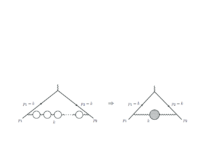
Рис. 1: Left panel: radiative corrections to the electromagnetic lepton vertex with insertions of the vacuum polarisation operator with an arbitrary number of lepton loops. Right panel: the second order diagram representing the set of graphs depicted in the left panel as exchanges of one massive photon.

II THEORETICAL FRAMEWORK

The main idea of the approach is to apply the dispersion relations to the corresponding Feynman diagram to express it via the Feynman $\displaystyle x$-parametrization of the second-order diagram with massive photons and finally to apply the Mellins–Barnes representation to the massive photon propagator (see Fig. 1 as the illustration) and again the dispersion relations to the polarisation operators of the internal lepton $\displaystyle\ell\neq L$ different from the external one. In this way, one can express any diagram from the mentioned subset in a rather simple form as a comvolution integral of two Mellin momenta (for details, cf. Ref. Solovtsova23 ). Then the QED corrections to the lepton anomalous magnetic moment due to bubble-like Feynman diagrams with the insertion of the photon polarization operator with an arbitrary number $\displaystyle n=p+j$ of loops, where $\displaystyle p$ is the number of loops formed by leptons $\displaystyle L$ of the same type as the external one, $\displaystyle j$ denotes the leptons $\displaystyle\ell\neq L$, has the form

$$\displaystyle a_{L}(p,j)=\frac{\alpha}{\pi}\frac{F_{(p,j)}}{2\pi i}\int\limits_{c-i\infty}^{c+i\infty}ds\;\left(\frac{4m_{\ell}^{2}}{m_{L}^{2}}\right)^{-s}\Gamma(s)\Gamma(1-s)\;\left(\frac{\alpha}{\pi}\right)^{p}\Omega_{p}(s)\left(\frac{\alpha}{\pi}\right)^{j}R_{j}(s),$$

(1)

where the factor $\displaystyle F_{(p,j)}$ is related to the binomial coefficients $\displaystyle C_{p+j}^{p}$ as $\displaystyle F_{(p,j)}=(-1)^{p+j+1}C_{p+j}^{p}$. Explicitly, the Mellin momenta $\displaystyle\Omega_{p}(s)$ and $\displaystyle R_{j}(s)$ read as

$$\displaystyle\left(\frac{\alpha}{\pi}\right)^{p}\Omega_{p}(s)=\int_{0}^{1}dx\;x^{2s}(1-x)^{1-s}\left[\Pi^{(L)}\left(-\frac{x^{2}}{1-x}m_{L}^{2}\right)\right]^{p},$$ (2)

$$\displaystyle\left(\frac{\alpha}{\pi}\right)^{j}R_{j}(s)=\int_{0}^{\infty}\frac{dt}{t}\left(\frac{4m_{\ell}^{2}}{t}\right)^{s}\frac{1}{\pi}\mbox{\rm Im}\left[\Pi^{(\ell)}(t)\right]^{j}.$$ (3)

Below we consider the case when $\displaystyle p=0$ and $\displaystyle j=4$ (see Fig. 2).

Contribution of the diagram with four identical lepton loops

Рис. 2: Vacuum polarization diagram with insertion of four identical lepton loops formed by leptons other than the external one.

Using Eqs. (1) – (3), the contribution to the lepton anomaly from the diagram shown in Fig. 2 can be written as

$$a_{L}^{\ell\ell\ell\ell}(r)\equiv A_{2,L}^{(10),\ell\ell\ell\ell}(r)\left(\frac{\alpha}{\pi}\right)^{5}=\left(\frac{\alpha}{\pi}\right)^{5}\frac{1}{2\pi i}\int\limits_{c-i\infty}^{c+i\infty}r^{-2s}{\cal F}(s)ds\,,$$ (4)

where the integrand $\displaystyle{\cal F}(s)$ looks like

$${\cal F}(s)=\left\{\frac{Z_{1}(s)}{729}-(1+s)Z_{2}(s)\left[\frac{81\pi^{2}}{729}-\frac{2}{3}\;\psi^{(1)}(s)\right]\right\}\frac{4\pi^{2}(1-s)}{Y(s)\sin^{2}(\pi s)}\,.$$ (5)

For the sake of brevity the following notation has been introduced

$$\displaystyle Z_{1}(s)=1259712+955332s-4110912s^{2}-6558755s^{3}-1384529s^{4}$$ (6)

$$\displaystyle\leavevmode\nobreak\ +3898617s^{5}+3867513s^{6}+1653510s^{7}+373944s^{8}+43520s^{9}+2048s^{10},$$

$$\displaystyle Z_{2}(s)=-8400-26340s-22144s^{2}+1641s^{3}+11729s^{4}+6894s^{5}+$$

$$\displaystyle\leavevmode\nobreak\ \leavevmode\nobreak\ \leavevmode\nobreak\ \leavevmode\nobreak\ \leavevmode\nobreak\ \leavevmode\nobreak\ \leavevmode\nobreak\ \leavevmode\nobreak\ +1835s^{6}+237s^{7}+12s^{8},$$ (7)

$$\displaystyle Y(s)=s(s+1)^{2}(s+2)^{2}(3+s)(4+s)(5+s)(6+s)(1+2s)(3+2s)$$

$$\displaystyle\leavevmode\nobreak\ \leavevmode\nobreak\ \leavevmode\nobreak\ \leavevmode\nobreak\ \leavevmode\nobreak\ \leavevmode\nobreak\ \times(5+2s)(7+2s).$$ (8)

As the integrand (5) is singular, then the integral (4) can be carried out by the Cauchy residue theorem closing the integration contour in the left ($\displaystyle r<1$) or right ($\displaystyle r>1$) semiplanes of the Mellin complex variable $\displaystyle s$ and computing the corresponding residues in these domains.

Case $\displaystyle r>1$. By closing the contour of integration to the right and computing the corresponding residues in this domain, we get the following result:

$$\displaystyle A_{2,L}^{(10),\ell\ell\ell\ell}(r>1)=\;D_{0}(r)+2D_{1}(r)\ln(r)+D_{2}(r)\bigg{[}{\rm Li}_{2}\left(\frac{1}{r^{2}}\right)-2\ln\left(1-{\frac{1}{r^{2}}}\right)$$

$$\displaystyle\times\ln(r)\bigg{]}-\frac{16}{9}\left(\frac{8r^{2}}{75}+5r^{4}+\frac{2\pi^{2}r^{4}}{3}\right)\left[{\rm Li}_{2}\left(\frac{1}{r^{2}}\right)\ln(r)+{\rm Li}_{3}\left(\frac{1}{r^{2}}\right)\right]+\Sigma_{1}(r),$$ (9)

where Li_n is the polylogarithm function of the order $\displaystyle n$ and the polynomials $\displaystyle D_{0-2}(r)$ are defined as follows

$$\displaystyle D_{0}(r)=\;-\frac{14463825527}{11252115000}-\frac{143175013r^{2}}{14033250}+\frac{680597537r^{4}}{63149625}+\frac{97213348r^{6}}{63149625}+\frac{797842r^{8}}{2338875}\quad$$

$$\displaystyle\leavevmode\nobreak\ +\frac{42952r^{10}}{1002375}+\frac{\leavevmode\nobreak\ \pi^{2}}{2}r\left(\frac{18203}{31185}+\frac{28010r^{2}}{5103}-\frac{5957r^{4}}{2025}-\frac{12916r^{6}}{70875}\right)-\pi^{2}\left(\frac{57419}{255150}\right.$$

$$\displaystyle\left.-\frac{2878}{2679075r^{2}}-\frac{1251149r^{2}}{1559250}-\frac{249589r^{4}}{841995}-\frac{40591r^{6}}{336798}-\frac{3632r^{8}}{93555}-\frac{64r^{10}}{13365}\right)+2r\bigg{[}\frac{18203}{31185}$$

$$\displaystyle+\frac{28010r^{2}}{5103}-\frac{5957r^{4}}{2025}-\frac{12916r^{6}}{70875}-\pi^{2}\left(\frac{18203}{748440}+\frac{2801r^{2}}{13608}-\frac{23r^{4}}{216}-\frac{7r^{6}}{1080}\right)\bigg{]}$$

$$\displaystyle\times\bigg{[}{\rm Li_{2}}\left(\frac{1-r}{1+r}\right)-{\rm Li_{2}}\left(-\frac{1-r}{1+r}\right)\bigg{]}+\frac{\leavevmode\nobreak\ \pi^{4}}{2}r\left(\frac{18203}{748440}+\frac{2801r^{2}}{13608}-\frac{23r^{4}}{216}-\frac{\leavevmode\nobreak\ 7r^{6}}{1080}\right),$$

$$\displaystyle D_{1}(r)=\;\frac{9239297}{26790750}+\frac{15360524r^{2}}{5011875}-\frac{109392281r^{4}}{21049875}-\frac{26671558r^{6}}{21049875}-\frac{2468692r^{8}}{7016625}$$

$$\displaystyle-\frac{42952r^{10}}{1002375}+\pi^{2}\left(\frac{25}{243}-\frac{1185953r^{2}}{1871100}-\frac{4624r^{4}}{40095}-\frac{26501r^{6}}{224532}-\frac{416r^{8}}{10395}-\frac{64r^{10}}{13365}\right),$$

$$\displaystyle D_{2}(r)=\;\frac{8}{175}+\frac{13664r^{2}}{10125}+\frac{1274r^{4}}{729}-\frac{1568r^{6}}{1215}+\frac{410r^{8}}{567}+\frac{42152r^{10}}{127575}+\frac{42952r^{12}}{1002375}$$

$$\displaystyle\leavevmode\nobreak\ \leavevmode\nobreak\ \leavevmode\nobreak\ \leavevmode\nobreak\ \leavevmode\nobreak\ \leavevmode\nobreak\ \leavevmode\nobreak\ \leavevmode\nobreak\ \leavevmode\nobreak\ +\pi^{2}\left(\frac{2}{\leavevmode\nobreak\ 81}-\frac{8r^{2}}{27}+\frac{34r^{4}}{81}-\frac{64r^{6}}{405}+\frac{16r^{8}}{189}+\frac{\leavevmode\nobreak\ \leavevmode\nobreak\ 64r^{10}}{1701}+\frac{64r^{12}}{13365}\right).$$

Finally, the last term in Eq. (Contribution of the diagram with four identical lepton loops) is the sum associated with $\displaystyle\sin^{2}(\pi s)$ in the denominator of the function $\displaystyle{\cal F}(s)$:

$$\Sigma_{1}(r)=\;\frac{8}{3}\sum_{n=2}^{\infty}\left[\frac{C_{1}(n)}{Y(n)}\psi_{n}^{(1)}+(n-1)C_{2}(n)\left(2\psi_{n}^{(1)}\ln(r)-\psi_{n}^{(2)}\right)\right]\frac{r^{-2n}}{Y(n)}\,,$$ (10)

where

$$\displaystyle C_{1}(n)=\left(n+1\right)^{2}(n+2)\bigg{(}635040000+7687008000n+36734547600n^{2}$$

$$\displaystyle+93125888040n^{3}+135651027372n^{4}+104915891978n^{5}+10006706560n^{6}$$

$$\displaystyle-69851951805n^{7}-83164962406n^{8}-51439049641n^{9}-18649902420n^{10}$$

$$\displaystyle-2892341259n^{11}+812142446n^{12}+656337939n^{13}+212614912n^{14}$$

$$\displaystyle+42833116n^{15}+5711184n^{16}+493456n^{17}+25152n^{18}+576n^{19}\bigg{)}\,,$$ (11)

$\displaystyle C_{2}(n)=Z_{2}(s=n)$, $\displaystyle Z_{2}(s)$ and $\displaystyle Y(s)$ are given by Eqs. (7) and (8), respectively; $\displaystyle\psi_{n}^{(1,2)}$ denotes the polygamma functions of the first or the second order of the integer argument $\displaystyle n$.

Case $\displaystyle r<1$. It should be noted that calculating the integral (4) in the region $\displaystyle r<1$ is much more difficult compared to the case $\displaystyle r>1$. This is due to the presence of additional zeros for the function $\displaystyle Y(s)$, Eq. (8). Also, for negative arguments, the polygamma function $\displaystyle\psi^{(1)}(s)$ also has poles for integers $\displaystyle s=-n$. Having found all the residues and summed them up, we get

$$\displaystyle A_{2,L}^{(10),\ell\ell\ell\ell}(r<1)=P_{0}(r)+2P_{1}(r)\ln(r)+4P_{2}(r)\ln^{2}(r)+8P_{3}(r)\ln^{3}(r)$$

$$\displaystyle+\frac{4}{3}K_{1}\ln^{4}(r)-\frac{128}{135}r^{4}\ln^{5}(r)+2K_{3}\bigg{[}\Phi\left(r^{2},4,\frac{1}{2}\right)-2\Phi\left(r^{2},3,\frac{1}{2}\right)\ln(r)$$

$$\displaystyle+2\Phi\left(r^{2},2,\frac{1}{2}\right)\ln^{2}(r)\bigg{]}+\Sigma_{2}(r),$$ (12)

where $\displaystyle\Phi(r^{2},n,1/2)$ is the Lerch function, which is related to the polylogarithms as: $\displaystyle\Phi(r^{2},n,1/2)={2^{n-1}}\bigl{[}{\rm Li}_{n}(r)-{\rm Li}_{n}(-r)\bigr{]}/{r}.$ The notation $\displaystyle P_{i}(r)$ corresponds to the expressions

$$\displaystyle P_{0}(r)=\frac{64613}{26244}-\frac{145231r^{2}}{17325}+\frac{265354583r^{4}}{7016625}+\frac{5155111r^{6}}{1002375}+\frac{1644584209r^{8}}{261954000}$$

$$\displaystyle+\frac{262864711931r^{10}}{445583754000}-\frac{38750851857953r^{12}}{70020304200000}+\pi^{2}\left(\frac{317}{1458}-\frac{380911r^{2}}{173250}\right.$$

$$\displaystyle\left.+\frac{1224743r^{4}}{841995}-\frac{1473151r^{6}}{1559250}-\frac{9577847r^{8}}{61122600}+\frac{\leavevmode\nobreak\ 283177187r^{10}}{3713197950}\right.$$

$$\displaystyle\left.+\frac{\leavevmode\nobreak\ 55905529021r^{12}}{1283705577000}\right)-\pi^{2}K_{1}(r)\left({\rm Li}_{2}(r^{2})-\frac{\pi^{2}}{5}\right)+\frac{\pi^{2}}{2r}\left(K_{4}(r)-\frac{\pi^{2}}{3}K_{3}(r)\right)$$

$$\displaystyle-\frac{2}{r}\left(K_{4}(r)+\pi^{2}K_{3}(r)\right)\left[{\rm Li}_{2}\left(\frac{1-r}{1+r}\right)-{\rm Li}_{2}\left(-\frac{1-r}{1+r}\right)\right]-K_{5}(r){\rm Li}_{2}(1-r^{2})$$

$$\displaystyle-\left(\frac{100}{81}+\frac{128r^{2}}{675}+\frac{64r^{4}}{9}-\pi^{2}\frac{\leavevmode\nobreak\ 32r^{4}}{9}\right){\rm Li}_{3}(r^{2})+\left(6K_{2}(r)-\frac{128r^{4}}{675}\right.$$

$$\displaystyle\left.-\pi^{2}\frac{\leavevmode\nobreak\ 64r^{4}}{27}\right)\zeta(3)-2\left(K_{1}(r)+\frac{8}{27}\right){\rm Li}_{4}(r^{2})+\frac{128}{9}r^{4}\left({\rm Li}_{5}(r^{2})-\zeta(5)\right),$$

$$\displaystyle P_{1}(r)=\frac{8609}{4374}-\frac{2190631r^{2}}{280665}-\frac{\leavevmode\nobreak\ 139188328r^{4}}{7016625}-\frac{1590044r^{6}}{7016625}-\frac{27882949r^{8}}{9355500}$$

$$\displaystyle-\frac{1090421197r^{10}}{1768189500}+\frac{671218651r^{12}}{5051970000}+\pi^{2}\left(\frac{50}{243}-\frac{50399r^{2}}{41580}+\frac{6431r^{4}}{13365}\right.$$

$$\displaystyle\left.+\frac{20003r^{6}}{1871100}+\frac{5539r^{8}}{48510}-\frac{16846r^{10}}{5893965}-\frac{2119877r^{12}}{92619450}\right)+\left(\frac{50}{81}+\frac{64r^{2}}{675}+\frac{32r^{4}}{9}\right.$$

$$\displaystyle\left.-\pi^{2}\frac{16r^{4}}{9}\right){\rm Li}_{2}(r^{2})-\pi^{2}K_{1}(r)\ln(1-r^{2})+2K_{1}(r)\biggl{(}{\rm Li}_{3}(r^{2})+2\zeta(3)\biggr{)}$$

$$\displaystyle+\;\frac{4}{27}\;{\rm Li}_{3}(r^{2})-\frac{\leavevmode\nobreak\ 32r^{4}}{3}{\rm Li}_{4}(r^{2}),$$

$$\displaystyle P_{2}(r) \displaystyle= \displaystyle\;\frac{317}{486}-\frac{247663r^{2}}{62370}+\frac{2139227r^{4}}{561330}-\frac{40591r^{6}}{112266}-\frac{3632r^{8}}{31185}-\frac{64r^{10}}{4455}$$

$$\displaystyle+K_{1}(r)\left({\rm Li}_{2}(r^{2})-\frac{\pi^{2}}{3}\right)+\frac{32}{9}r^{4}\biggl{(}{\rm Li}_{3}(r^{2})-\zeta(3)\biggr{)},$$

$$\displaystyle P_{3} \displaystyle= \displaystyle\frac{25}{243}-\frac{231277r^{2}}{374220}-\frac{4624r^{4}}{40095}-\frac{26501r^{6}}{224532}-\frac{416r^{8}}{10395}-\frac{64r^{10}}{13365}-\pi^{2}\frac{\leavevmode\nobreak\ 16r^{4}}{81}$$

$$\displaystyle-\frac{16}{27}r^{4}\;{\rm Li}_{2}(r^{2})-\frac{1}{3}K_{1}(r)\ln(1-r^{2})-K_{3}(r)\frac{1}{3r}\bigl{[}\ln(1+r)-\ln(1-r)\bigr{]},$$

where $\displaystyle\zeta(x)$ denotes the Euler–Riemann zeta function of the argument $\displaystyle x$.

Finally, the sum $\displaystyle\Sigma_{2}(r)$ in Eq. (Contribution of the diagram with four identical lepton loops) reads as

$$\Sigma_{2}(r)=\frac{8}{3}\sum_{n=7}^{\infty}\left[\frac{\leavevmode\nobreak\ C_{1}(-n)}{Y(-n)}\psi_{n}^{(1)}+(n^{2}-1)Z_{2}(-n)\left(2\psi_{n}^{(1)}\ln(r)+\psi_{n}^{(2)}\right)\right]\frac{r^{2n}}{Y(-n)},$$ (13)

where the notations are the same as in the sum (10). For brevity, polynomials $\displaystyle K_{i}(r)$ in Eq. (Contribution of the diagram with four identical lepton loops) are introduced

$$\displaystyle K_{1}(r)=\frac{2}{27}-\frac{8r^{2}}{9}+\frac{34r^{4}}{27}-\frac{64r^{6}}{135}+\frac{16r^{8}}{63}+\frac{64r^{10}}{567}+\frac{64r^{12}}{4455}\,,$$

$$\displaystyle K_{2}(r)=\frac{50}{243}-\frac{104r^{2}}{81}-\frac{134r^{4}}{81}-\frac{4432r^{6}}{6075}-\frac{1033r^{8}}{2205}-\frac{12332r^{10}}{535815}+\frac{2119877r^{12}}{46309725}\,,$$

$$\displaystyle K_{3}(r)=\frac{18203r^{2}}{249480}+\frac{2801r^{4}}{4536}-\frac{23r^{6}}{6075}-\frac{7r^{8}}{360}\,,$$

$$\displaystyle K_{4}(r)=-\frac{\leavevmode\nobreak\ 2801r^{4}}{567}+\frac{230r^{6}}{81}+\frac{1813r^{8}}{10125}\,,$$

$$\displaystyle K_{5}(r)=-\frac{317}{243}+\frac{31664r^{2}}{10125}+\frac{167r^{4}}{729}-\frac{32r^{6}}{27}+\frac{56r^{8}}{81}+\frac{1640r^{10}}{5103}+\frac{3832r^{12}}{91125}\,.$$

III DISCUSSION

The above Eqs. (Contribution of the diagram with four identical lepton loops) and (Contribution of the diagram with four identical lepton loops) represent the exact analytical expressions of the tenth order of the radiative corrections from diagrams with the insertion of four identical lepton loops, as depicted in Fig. 2. Despite their cumbersomeness, the explicit analytical form allows for numerical calculations with any desired precision. The precision can only be limited by the knowledge of the basic physical quantities such as $\displaystyle\alpha$, $\displaystyle m_{\ell}$ and $\displaystyle m_{L}$.

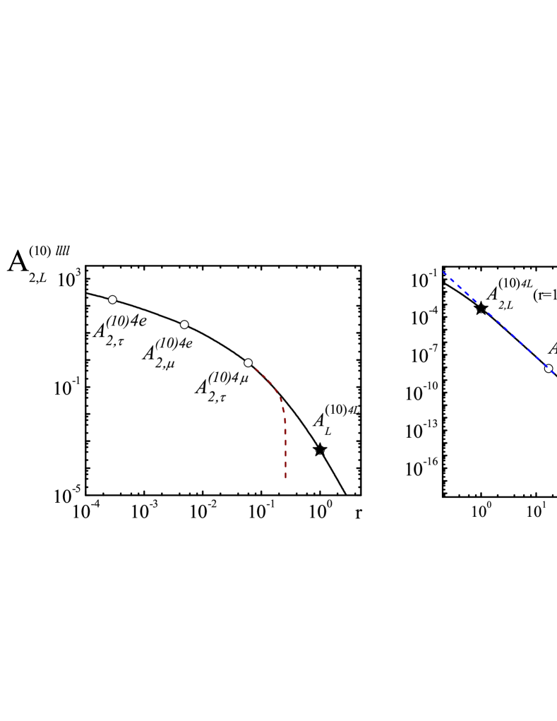
Рис. 3: Comparison of asymptotic expansions with exact calculations of the coefficient $\displaystyle A_{2}^{(10)}(r)$ The solid curve is the exact result, the dashed lines are the asymptotic for $\displaystyle r\ll 1$ (left panel) and $\displaystyle r\gg 1$ (right panel). The open circles, as well as the labels associated with them, point to physical values of the ratio $\displaystyle r$ and to the corresponding physical coefficients $\displaystyle A_{2,L}^{(10)\ell\ell\ell\ell}(r)$. The universal value $\displaystyle A_{2,L}^{(10)LLLL}(r)$ is displayed by the full star.

Let us briefly discuss asymptotic expansions of the coefficient $\displaystyle A_{2}^{(10),\ell\ell\ell\ell}$ considering the limits $\displaystyle r\ll 1$ and $\displaystyle r\gg 1$. A comparison of the result of calculating $\displaystyle A_{2}^{(10),\ell\ell\ell\ell}$ using asymptotic and exact formulas, Eqs. (Contribution of the diagram with four identical lepton loops) and (Contribution of the diagram with four identical lepton loops), is illustrated in Fig. 3, in which the solid curve is the exact result, and the dashed-dotted line is the asymptotic for $\displaystyle r\ll 1$ (left panel) and $\displaystyle r\gg 1$ (right panel). Note, we do not give here our expansion formula for the case $\displaystyle r\ll 1$ (see discussion below). For the case $\displaystyle r\gg 1$, using Eq. (Contribution of the diagram with four identical lepton loops), we get

$$\displaystyle A_{2,L}^{(10),\ell\ell\ell\ell}(r\gg 1) \displaystyle\simeq \displaystyle\;\left(-\frac{369904}{88409475}+\frac{4402}{109147}\;\zeta(3)\right)\frac{1}{\leavevmode\nobreak\ r^{4}}-\left(\frac{598587203}{82751268600}\right.$$ (14)

$$\displaystyle\left.\leavevmode\nobreak\ \leavevmode\nobreak\ \leavevmode\nobreak\ \leavevmode\nobreak\ \leavevmode\nobreak\ \leavevmode\nobreak\ \leavevmode\nobreak\ \leavevmode\nobreak\ \leavevmode\nobreak\ \leavevmode\nobreak\ \leavevmode\nobreak\ \leavevmode\nobreak\ \leavevmode\nobreak\ \leavevmode\nobreak\ \leavevmode\nobreak\ \leavevmode\nobreak\ -\frac{71960}{127702575}\zeta(3)\right)\frac{1}{\leavevmode\nobreak\ r^{6}}+{\cal{O}}\left(\frac{1}{r^{8}}\right)\,.$$

It is interesting to note that there are no logarithmic terms in this expration.

One can see from Fig. 3 that the approximate expansions practically coincide with the exact formulae in quite large intervals of $\displaystyle r$, namely $\displaystyle 0<r<0.2$ for the expansion $\displaystyle r\ll 1$ (left panel) and $\displaystyle 2<r<\infty$ for the expansion $\displaystyle r\gg 1$ (right panel), herewith both intervals include all the corresponding physical values of $\displaystyle a_{L}^{\ell\ell\ell\ell}$.

Let us return to the region $\displaystyle r\ll 1$ for which there are asymptotic expansions in the literature, see Refs. Aguilar:2008qj ; Laporta94 . Our asymptotic expansion completely coincides with the expansion given in Ref. Laporta94 , which, however, corresponds only to the order $\displaystyle O(r^{2})$. In the expansion Ref. Aguilar:2008qj , see Eq. (A9) in the Appendix, which is given up to the order $\displaystyle O(r^{5})$, we found two misprint: a different sign in the term $\displaystyle\frac{32}{27}r^{2}\ln^{4}(r)$ and in $\displaystyle-\frac{61}{27}\pi^{2}\zeta(5)r^{4}$ instead of 61 there is the number 64.

Thus, the present investigation has confirmed that the approach used here is a powerful tool for finding exact analytical expressions for the bubble-like diagrams contributions to the anomalous magnetic moment of leptons.

• (1) P. A. M. Dirac, The quantum theory of the electron, Proc. Roy. Soc. Lond. A 117, 619 (1928).
• (2) F. Jegerlehner, The anomalous magnetic moment of the muon, Springer Tracts Mod. Phys.  274, 693 (2017).
• (3) T. Aoyama et al. The anomalous magnetic moment of the muon in the Standard Model, Phys. Rep. 887, 1 (2020).
• (4) R. H. Parker, C. Yu, W. Zhong, B. Estey, H. M$\displaystyle\ddot{u}$eller, Measurement of the fine-structure constant as a test of the Standard Model, Science 360, 191 (2018).
• (5) L. Morel, Z. Yao, P. Clade, S. Guellati-Khelifa, Determination of the fine-structure constant with an accuracy of 81 parts per trillion, Nature 588, 61 (2020).
• (6) B. Abi et al. (Muon $\displaystyle g-2$ Coll.), Measurement of the positive muon anomalous magnetic moment to 0.46 ppm, Phys. Rev. Lett. 126, 141801 (2021).
• (7) D.P. Aguillard et al. (Muon $\displaystyle g-2$ Collaboration), Measurement of the positive muon anomalous magnetic moment to 0.20 ppm, Phys. Rev. Lett. 131, 141801 (2023).
• (8) J. S. Schwinger, On quantum electrodynamics and the magnetic moment of the electron, Phys. Rev.  73, 416 (1948).
• (9) S. Volkov, A method of fast calculaion of lepton magnetic moments in quantum electrodynamics, Phys. Part. Nucl. 53, 805 (2022).
• (10) E. E. Boos and A. E. Davydychev, A method of evaluation massive Feynman diagrams, Theor. Math. Phys. 89, 1052 (1991).
• (11) J. P. Aguilar, D. Greynat, and E. de Rafael, Asymptotics of Feynman diagrams and the Mellin–Barnes representation, Phys. Lett. B 628, 73 (2005).
• (12) A. V. Kotikov, S. Teber, Multi-loop techniques for massless Feynman diagram calculations, Phys. Part. Nucl. 50, 1 (2019).
• (13) I. Dubovyk, J. Gluza, and G. Somogyi, Mellin–Barnes integrals: A primer on particle physics applications, Lect. Notes Phys. 1008, 1 (2022).
• (14) J. P. Aguilar, E. de Rafael, and D. Greynat, Muon anomaly from lepton vacuum polarization and the Mellin-Barnes representation, Phys. Rev.  D 77, 093010 (2008).
• (15) O. P.. Solovtsova O.P., V.I. Lashkevich, L. P. Kaptari, Lepton anomaly from QED diagrams with vacuum polarization insertions within the Mellin–Barnes representation, Eur. Phys. J. Plus. 138. 212 (2023).
• (16) S. Laporta, Analytical and numerical contributions of some tenth-order graphs containing vacuum polarization insertions to the muon $\displaystyle(g-2)$ in QED, Phys. Lett. B 328, 522 (1994).