Phase Diagram of growth modes in Graphene Growth on Cooper by Vapor Deposition
Abstract
Understanding the atomistic mechanism in graphene growth is crucial for controlling the number of layers or domain sizes to meet practical needs. In this work, focusing on the growth of graphene by chemical vapor deposition on copper substrates, the surface kinetics in the growth are systematically investigated by first-principles calculations. The phase diagram, predicting whether the growth mode is monolayer graphene or bilayer graphene under various experimental conditions, is constructed based on classical nucleation theory. Our phase diagram well illustrates the effect of high hydrogen pressure on bilayer graphene growth and clarifies the mechanism of the most widely used experimental growth approaches. The phase diagram can provide guidance and predictions for experiments and inspires the study of other two-dimensional materials with graphene-like growth mechanisms.
I \@slowromancapi@. Introduction
Graphene has sparked a wave of interest as a zero-bandgap two-dimensional material since its first successful exfoliationNovoselov et al. (2004). Exceptional electronic properties and impressive stability make it one of the most remarkable materials in electronic and energy-storage applicationsMorozov et al. (2008); Lee et al. (2008); Briggs et al. (2010). The properties of graphene strongly depends on the number of layers and the stacking orderYao et al. (2022a); Cai and Yu (2021). Graphene monolayer exhibits excellent charge carrier mobility and optical transmittance, making it a promising candidate for applications in optoelectronic memory devices, electrodes and solar cellsBolotin et al. (2008); Nair et al. (2008); Bae et al. (2010); Wang et al. (2014); Xia et al. (2009); Yu et al. (2015). Stacking of two or more graphene monolayers may lead to the emergence of novel physical properties, including tunable transport and optical propertiesZhang et al. (2009); Mak et al. (2009); Wang et al. (2008); Yin et al. (2016), as well as the Mott insulating stateCao et al. (2018a) and superconductivityCao et al. (2018b). Thus it is crucial to control the number of layers and the stacking order in graphene growth for large-scale practical applications. Understanding the growth mechanism of graphene with different layers is essential for achieving controllable graphene growth.
Diverse growth methods have been developed to achieve the controllable growth of grapheneHernandez et al. (2008); Shih et al. (2011); Nyakiti et al. (2012); Virojanadara et al. (2008); Liu et al. (2012a). Due to the ease of operation and a wide window of growth parameters, chemical vapor deposition (CVD) has an advantage over the complex and low-productivity exfoliation-stacking methodShih et al. (2011); Hernandez et al. (2008), as well as the costly SiC sublimation methodVirojanadara et al. (2008); Nyakiti et al. (2012). In CVD growth of graphene, methane gas commonly serves as the carbon source with transition metals acting as the substrateSeah et al. (2014). Among the transition metals, copper is preferable due to its low carbon solubility making layer control easierLópez and Mittemeijer (2004); Li et al. (2009a, b); Edwards and Coleman (2012). The deposited carbon source gas first decomposes into active carbon precursors, catalyzed by the metal substrate. Then the nucleation and growth proceed, the mechanism of which depends on the kinetic processes of the active carbon precursors.
Normally, the conventional thin film growth can be described as the - mode, in which the nucleation of new layers occurs on top of the lower oneLi et al. (2009c); Ding et al. (2003). However, the - (IWC) growth mode has been revealed in low-pressure CVD experiments during the bi-layer graphene (BLG) growth processNie et al. (2012); Fang et al. (2013); Li et al. (2013); Chan et al. (2018a). In this growth mode, the second layer graphene nucleates beneath and grows in competition with the first layer. The growth of the first layer would lead to a decrease in catalytic surface area and a shortage of carbon precursors, thereby inhibiting the growth of the second layer, which is known as the self-limiting growth. Moreover, the second layer would cease to grow due to the shortage of carbon precursors once the substrate is fully covered by the first layer.
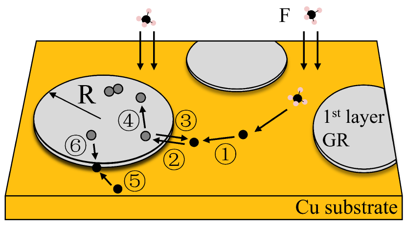
The unique graphene growth mechanism originates from the competing surface kinetic processes. Fig. 1 illustrates the surface kinetic processes involved in BLG growth, assuming that the growth unit is solely the C monomer. These processes can be divided into two categories. The first category includes the surface diffusion processes, namely on the clean substrate (1), across the step edge of the first layer graphene to the graphene-substrate interface (2) and the inverse one (3), and at the graphene-substrate interface (4). The second category involves the attachment processes that promote the growth of the first layer. They are labeled as 5 and 6, denoting the attachment to the first layer graphene from the uncovered region of the substrate and the graphene-Cu interface, respectively.
Many studies on the surface kinetics of graphene growth have focused on processes 1 and 5, providing insights into single layer graphene (SLG) growthWu et al. (2010); Li et al. (2017); Gao et al. (2011a, b); Kim et al. (2012); Chen et al. (2015, 2010); Riikonen et al. (2012); Wu et al. (2015); Andersen et al. (2019). Beyond SLG growth, Zhang et al. conducted extensive calculations on the possible kinetic processes near the boundary of graphene island, and reported a much lower barrier of process 2 at the H-terminated graphene edge, which is favorable for BLG growthZhang et al. (2014). Wei et al. also investigated the underlying atomistic mechanisms for BLG growth. They identified the critical island size required for the nucleation of the second layer and re-emphasized the effect of hydrogen gas on BLG growthChen et al. (2015). However, a generic growth model that can serve as a guide for experiments under various conditions has not yet been developed.
In this paper, the surface kinetic properties of C monomers on Cu(111) surface are systematically investigated using first-principles calculations. Based on the full understanding of the surface kinetics, a phase diagram of graphene growth modes is constructed according to the classical nucleation theory. Using the phase diagram, the conditions for BLG growth are determined and the growth mechanisms of commonly used growth techniques are elucidated. This work would motivate further investigations into the IWC growth mechanism of other 2D materials.
II \@slowromancapii@. Models Methods
The calculations are based on density functional theory (DFT) in the Perdew-Burke-Ernzerhof generalized gradient approximation (GGA-PBE) using the Vienna Ab initio Simulation Package (VASP), with Projector-Augmented Wave (PAW) methodsKresse and Furthmüller (1996a, b); Perdew et al. (1996); Blochl (1994). The semiempirical approach DFT-D2 is used to include the van der Waals (vdW) interactionsBučko et al. (2010). A cutoff energy of 650 eV for the plane wave basis set is employed for all calculations. The Cu(111) substrate is constructed based on the bulk Cu with an optimized lattice parameter of 3.634 Å. Three slab models (M1-M3) are used for different aims in the simulation. The bare Cu(111) surface is modelled by a (55) supercell consisting of a 5-layer slab and a 15 Å vacuum layer (M1). The Cu(111) surface partially covered by graphene is modelled by a Cu substrate of (94) supercell plus a (34) graphene supercell on top of the Cu substrate (M2). The Cu(111) surface fully covered by graphene is modelled by introducing an additional (55) graphene monolayer on the Cu substrate of (55) supercell (M3). The graphene is streched slightly to match the lattice parameter of the Cu substrate in M2 and M3.
The in-plane Brillon zones of the (55) supercell(M1/M3) and the (94) supercell(M2) are sampled by a -centered 33 mesh and a -centered 24 mesh, respectivelyMethfessel and Paxton (1989). The bottom two layers of Cu slabs are fixed to mimic the bulk in all three models. The relaxations are carried out until forces on the free atoms are converged to 0.01 eV/Å for structural optimizations. The energy barriers of the kinetic processes are calculated by the climbing image nudged elastic band (CI-NEB) method with the forces on the free atoms converged to 0.02eV/ÅHenkelman et al. (2000). These settings ensure a convergence in total energy of 0.1 meV/atom.
III \@slowromancapiii@. Surface kinetics
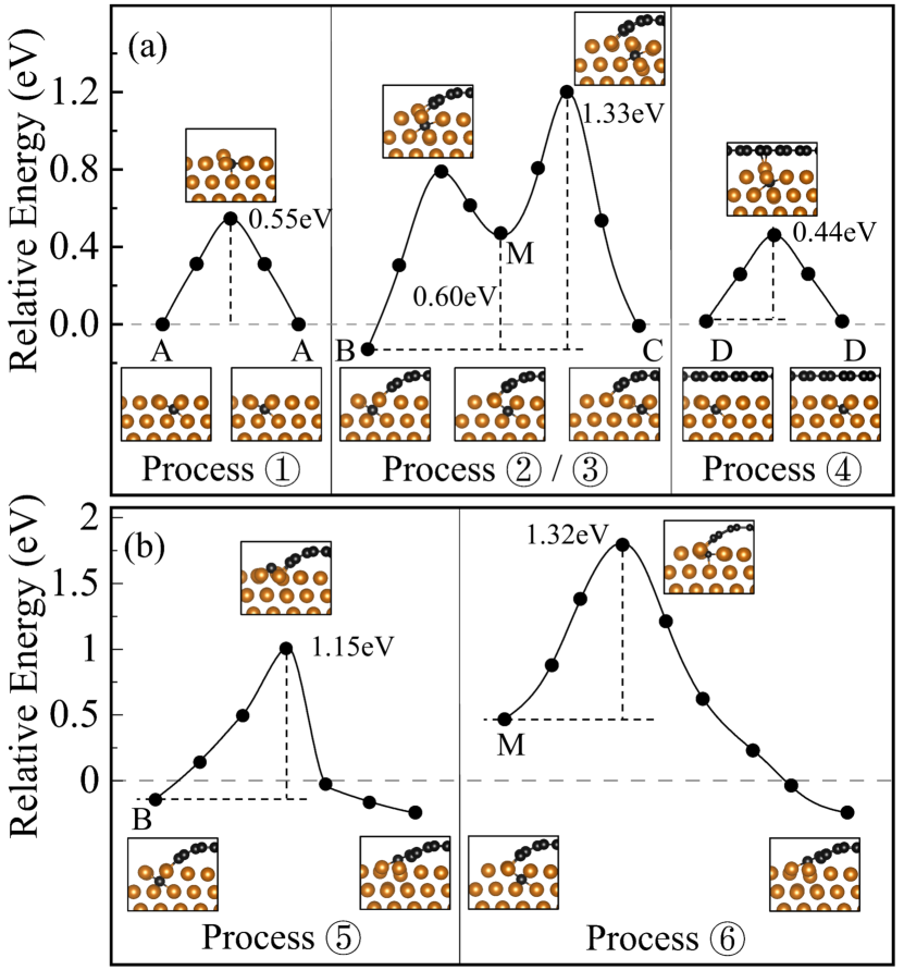
The main surface kinetic processes involved in the growth of BLG on Cu(111) substrates are shown in Fig. 1. It is widely accepted that the C monomer is more stable on the subsurface of the Cu(111) substrate than on the surfaceZhang et al. (2014); Chen et al. (2015, 2010); Riikonen et al. (2012); Wu et al. (2015); Andersen et al. (2019). Using model M1, our calculations indicate that the former is energetically favored by about 0.5eV. Therefore, we denote the adsorption site on the subsurface of Cu(111) as and set it as a reference for adsorption energies at other sites. Based on the calculations using model M2, the adsorption of a C monomer near the edge of graphene islands becomes energetically more favorable. The energy gain is about 0.14 eV () or 0.01 eV (), depending on whether the adsorption site is outside or inside the graphene covered zone. In contrast, when the adsorption site is located beneath the graphene islands but far from the edge (), the calculation using model M3 shows that it becomes energetically less favorable by 0.02 eV.
The difference in adsorption energy at different sites () mainly arises from the substrate deformation induced by adsorption. The adsorption of a C monomer on the subsurface of a Cu(111) substrate leads to a local expansion near the adsorption site. At the proximity of the graphene islands, the interaction between the graphene edges and the substrate slightly lifts the surface Cu atoms. Therefore, the substrate exhibits less deformation after the adsorption of C monomer at and than at , resulting in a lower adsorption energy. The adsorption of a C monomer at site costs more energy than at because the fully covered graphene inhibits the relaxation of the surface Cu atoms.
We then focus on the four diffusion processes of C monomers. As shown in Fig. 2(a), C monomers tend to diffuse on the subsurface of the Cu substrate, regardless of whether it is covered by graphene or not. The diffusion barriers on the uncovered and graphene fully covered Cu substrate are eV and eV, respectively. In comparison, the diffusion across the edge of the graphene island has a relatively high barrier. The energy barrier from the uncovered substrate to the graphene-covered substrate is eV, and the barrier of the reverse process is eV. The higher barrier across the edge can be attributed to the interaction between the dangling bonds of the graphene edge and the metal substrate. This interaction is also manifested by the bending of the graphene edge towards the substrate, as shown in the inset geometry configurations of Fig. 2(a).
Next, we investigate the attachment processes on the substrate. As shown in Fig. 2(b), the C monomer needs to overcome a barrier of eV to attach to the graphene edge from the uncovered substrate side, slightly less than the edge diffusion barrier . For process 6, the C monomer preferentially diffuses outward from beneath the graphene islands and then attaches to the edge. For comparison, we still obtain a direct attachment barrier of eV by imposing restrictions on the pathways of the C monomer.
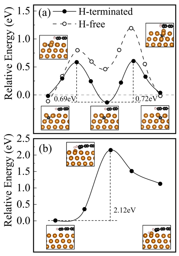
We now examine the impact of hydrogen gas on the surface kinetics during graphene growth. H atoms are highly involved in graphene growth as hydrogen gas is comparatively easier to decompose than methaneZhang et al. (2014). H atoms can saturate the edges of the first-layer graphene islands, reducing the interaction between the graphene edge and the substrate. This change facilitates the diffusion of C monomers across the island edge. As shown in Fig. 3(a), the H termination of edges reduces the diffusion barriers and to 0.72 eV and 0.69 eV, respectively. Meanwhile, the diffusion barriers of and remain nearly unaffected by the H termination of edges. On the other hand, the detachment of H atoms is a prerequisite condition for the attachment processes at the H-terminated edge. Fig. 3(b) shows that the barrier for H atom detachment from the H-terminated edge is 2.12 eV, which is higher than the attachment barriers and . Therefore, the detachment of H atom from edges becomes the rate-limiting step for the growth of the first-layer graphene islands. It is much easier for C monomers to accumulate beneath the first-layer islands under high hydrogen pressure due to the difficulty of attachments, which increases the probability of second layer nucleation.
There have been many studies on the simulation of the kinetic properties of C monomers. The value of in the current work is in agreement with the reported barriers of C monomer diffusion on Cu substrateWu et al. (2010); Chen et al. (2010, 2015); Riikonen et al. (2012); Wu et al. (2015); Li et al. (2017). The value of in the current work is higher than the reported results, which are approximately 0.3 eV.Zhang et al. (2014); Chen et al. (2015); Li et al. (2017). This difference possibly results from the larger (55) supercell used in our calculation. Besides, the previous work has investigated the processes that occur at the edges of islands, as well as the effect of H-terminated edges on these barriers. The reported hopping barriers of processes near the edge are slightly smaller than our resultsZhang et al. (2014); Li et al. (2017). This difference may originate from the tensile strain in the graphene introduced by the Cu substrate in our calculations, as we have demonstrated that a larger lattice of the system leads to a higher barrier for the same kinetic path.
IV \@slowromancapiv@. Phase diagram
IV.1 A. Concentrations of C monomers
With a complete understanding of the surface kinetic processes involved in growth, we are able to achieve deeper insights into the graphene growth mode using rate equation approaches. Two approximations are used in our model. Firstly, we ignore the details of gas decomposition and assume the C monomers arrive at the substrate at a fixed deposition rate of per in the normal direction, where is the area of an adsorption site on the substrate. It is noteworthy that the deposition rate on the region covered by C clusters is zero, as the gas decomposition requires the aid of the catalytic substrate in experiments. Secondly, we assume the growth unit is the C monomer and its mean residence time before desorption is long enough to incorporate into clusters. As shown in Fig. 1, we start with a model where circular first-layer graphene islands have formed on the Cu substrate. The average radius of the first-layer islands and half of the average island-island separation are denoted as and , respectively, both in units of .
The deposited C monomers can diffuse across or attach to the boundary of the first-layer graphene islands. The corresponding rate of the six processes is given by , where is the kinetic barrier of process , is the attempt frequency, is the Boltzmann constant and is the experimental temperature. It is reasonable to assume that the growth is limited by the attachment, since the kinetics of diffusion processes are much more rapid. In this case, the steady-state C monomer concentration is easily reached.
According to the rate equation, the steady-state concentration of C monomer beneath the first-layer graphene islands remains constant due to the absence of direct atomic deposition at the graphene-substrate interface. We denote this concentration as , which also represents the probability of an adsorption site beneath the first-layer graphene islands being occupied by a C monomer. On the contrary, the steady-state concentration of C monomer outside the graphene islands is position-dependent, influenced by the deposition rate and diffusion kinetics. Here we are only interested in the C monomer concentration at the edge outside the graphene islands, which is denoted as .
The total number of C monomers beneath the first-layer graphene islands is only affected by the kinetic processes 2, 3 and 6. Therefore, it evolves as follows,
| (1) |
The steady-state value of at a certain first-layer island radius remains constant over time, which gives
| (2) |
Similarly, the steady-state value of the total number of C monomers on the exposed Cu substrate is also constant if only the first-layer radius is fixed. Therefore, the deposited atoms contribute solely to the growth of first-layer islands at steady state and fixed , which follows that
| (3) |
On the other hand, the first-layer islands expand in size through the attachment processes 5 and 6 according to the boundary condition. It gives that
| (4) |
Combining Eq. (2) - (4), we have
| (5) |
and the number of C monomers beneath the first-layer graphene islands at steady state is
| (6) |
where
| (7) |
As shown in Eq. (7), is merely determined by the surface kinetics while depends on both the surface kinetics and the deposition rate. In this way, the complicated surface kinetic properties and growth conditions are described by the two dimentionless factors and . Such reduction makes the growth phase diagram possible. Specifically, by using the kinetic results in Sec. \@slowromancapiii@, we have and for the experiments under low and high partial pressure at K, respectively.
| (eV) | (eV) | (eV) | ||||
| 1 | 0 | 0 | 0 | 1.18 | 22.54 | |
| 2 | 1.20 | 0.43 | -0.77 | 0.09 | 3.15 | |
| 3 | 1.11 | 0.29 | -0.82 | 0.07 | 8.94 | |
| 4 | 1.31 | 0.63 | -0.68 | 0.03 | 1.55 | |
| 5 | 1.33 | 0.70 | -0.63 | 0.02 | 4.35 | |
| 6 | 1.38 | 0.77 | -0.61 | 0.01 | 4.76 |
IV.2 B. Monomers beneath islands
The nucleation of second-layer islands is more favorable if is larger than the size of a critical nucleus . Therefore, a rough estimation of is necessary in order for preliminary screening of the conditions for BLG growth.
According to Eq. (6), has a maximum value of at . The half of the island-island separation is correlated with the concentration of first-layer nuclei by . In some situations the nucleation density is controlled by seeds or specific templatesHao et al. (2013), making the size of case-by-case. Here we assume the more general spontaneous nucleation. In this case, the first-layer nuclei have a saturation concentration and thus depends on as followsVenables (1973); Venables et al. (1984),
| (8) |
where is a proportional coefficient. Therefore, we obtain the maximum value of the total C monomers beneath the first-layer island as follows,
| (9) |
According to the classical nucleation theory (See Supplementary Material), the expression of is as follows,
| (10) |
where is the average binding energy per atom of the first-layer critical nucleus, is the coverage when the nucleus density is saturated, and are the average number of attachment sites of a critical nucleus and stable nucleus, respectively. By setting K, , , , and adapting the binding energies reported by Zhong et al.Zhong et al. (2016), the values of for are listed in Table 1.
Combining Eq.(8) - Eq.(10), we can determine the range of that satisfies . For , it requires that is smaller than . For , is always smaller than . For , it requires that is larger than or 10 for H-free or H-rich situations, respectively. In the typical experimental nucleation density range of 10 mm-2 (See Supplementary Material), is approximately within Zhao et al. (2016); Chan et al. (2018a). Thus BLG growth is possible when first-layer graphene islands are terminated by H atoms for a critical nucleus size .
IV.3 C. Second Layer Nucleation
We now consider the second-layer nucleation beneath the first-layer graphene islands, assuming the critical size of the second-layer nucleus is still , the same as the first-layer nucleus. According to the classical nucleation theory, the nucleation rate per unit area can be written as , where is the concentration of clusters of size at steady stateVenables (1973); Venables et al. (1984). The expression of is given by , where is the average binding energy per atom of the second-layer critical nucleusWalton (1962).
Obviously, the number of second-layer nuclei increases as the first-layer islands grow, until equals to and the first-layer islands coalesce. Subsequently, the growth unit is no longer supplied due to the absence of exposed catalytic substrate. The upper limit of the nucleus number beneath the first-layer graphene islands can thus be obtained as , where represents the minimal radius of the well-defined first-layer graphene island from which the second-layer nucleation begins to form. For a nucleus with a radius , its size . Here we choose the minimal first-layer island involved in the second-layer nucleation as the C24 cluster containing seven 6-membered rings, which means . Combining with Eq. (3), we have
| (11) |
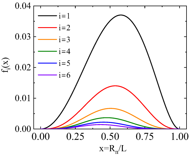
where and the proportional coefficient . Here , and denotes the difference in the average binding energies per atom of the critical nuclei at the graphene-substrate interface and on the Cu substrate. A negative indicates that the cluster is more favorable to form on the bare substrate than beneath the first-layer graphene islands. By using the forementioned values and setting based on the kinetic properties obtained in Sect. \@slowromancapiii@, the values of for are listed in Table 1. The expressions of for are also listed in Table 1. Fig. 4 shows the variation of with . It can be identified that reaches its maximum at a moderate value of . Therefore, the number of second-layer nuclei has a maximum at a moderate nuclei concentration. As for the effects of the parameters and on , it is noteworthy that is inversely proportional to the dimensionless factor , while the influence of on is mediated by and .
IV.4 D. Growth Modes
The growth mode can now be estimated according to the value of . If , there is little possibility that a second-layer nucleus forms before the coalescence of first-layer islands. Only if , the second-layer nucleation will occur and the BLG growth becomes possible. Therefore the condition gives the border between SLG growth and BLG growth. The phase diagram of the growth mode can thus be constructed using the values in Table 1.
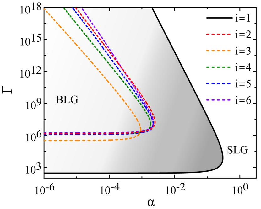
We first consider the simplest situation of as the binding energy is zero. The black solid line in Fig. 5 represents the border curve of BLG and SLG growth when , which divides the diagram region into two sections. The gradient-filled area in the top left corner of the diagram is suitable for BLG growth, while the remaining colorless area only permits SLG growth. The diagram is very similar to the one that predicts the layer-by-layer growth and island growth we reported beforeShu et al. (2017), indicating that the IWC growth is analogous to the interfacial growth.
Now it is easy to identify the influence of the reduced parameter on the growth mode. As shown in Fig. 5, only SLG growth occurs when is larger than a critical value. When is smaller than the critical value, BLG growth can occur within a moderate range of whereas SLG growth is reentrant when the value of is sufficiently small or large. Furthermore, the range of for BLG growth becomes larger for smaller , indicating that a larger favors SLG growth while a smaller favors BLG growth. According to Eq. (7), a larger value of implies more rapid attachment kinetics at the island edge or more sluggish diffusion into the graphene-covered area. Therefore, the concentration of C monomers beneath the first-layer graphene islands is always deficient to form the second-layer nucleus, resulting in the advantage of SLG over BLG. Conversely, a smaller generally indicates a smaller attachment kinetic rates as well as a smaller outward diffusion rate than the intralayer diffusion rate, which favors the BLG growth.
The influence of on the growth mode is nonmonotonic. As discussed above, the SLG growth occurs only for a very small or large value of if is not large enough. The growth of SLG at small corresponds to a very high density of first-layer nuclei, so that the second-layer nucleation hardly occurs before the coalescence of the first-layer islands. Conversely, the SLG growth at large is mediated by the low second-layer nucleation rate due to the low concentration of C monomers.
The size of the critical nucleus varied with the growth condition also influences the growth mode. When , the value of is no longer zero and the coefficients and become dependent on the temperature. The border curves for at K are represented by the colored dashed curves in the phase diagram. The shrinkage of BLG growth area with larger originates mostly from the negative that results into smaller and smaller nucleation number . There is little variations among the border curves for , with an exception of because the magnitude of is largest than the others. It suggests an additional way to regulate the growth mode by tuning the binding energy of nuclei through substrate engineering.
V \@slowromancapv@. Discussion
In the framework of the phase diagram, some strategies can be predicted to control the growth process. For instance, BLG growth can be intentionally selected based on three strategies. Firstly, a relatively low value of is beneficial, as illustrated in the diagram. The value of can be decreased by reducing the interaction between the edges of graphene islands and the substrate. For example, hydrogen termination of edges can reduce the value of from to based on our calculations. Secondly, a moderate value of is beneficial for BLG growth. Therefore, it is crucial to pay close attention to the gas flux and the deposition rate in experiments. Finally, enlarging the area of BLG growth in the diagram by changing the border is also a strategy for BLG growth. A possible approach is to increase through substrate modification, which would enhance the coefficient and thus the BLG growth area in the phase diagram.
Up to now, many experiments have reported good yields of both SLG and BLG. Single crystal SLG has been successfully grown in experiments by dynamically controlling the gas ratio or pressureLi et al. (2010); Chan et al. (2013); Chaitoglou and Bertran (2016); Sun et al. (2016); Wu et al. (2016); Zhou et al. (2013); Guo et al. (2016), domain orientation controlChen et al. (2012); Shi et al. (2021), or pretreating the substrate through coatingLuo et al. (2017), annealingNguyen et al. (2019); Luo et al. (2019), polishingYao et al. (2022b); Braeuninger-Weimer et al. (2016), alloyingHuang et al. (2018); Liu et al. (2018) or oxidizingSun et al. (2021a); Zhou et al. (2013); Srinivasan et al. (2018); Gan and Luo (2013); Eres et al. (2014); Hao et al. (2013). The key points in these methods are suppressing nucleation density and improving growth rate while the self-limiting growth regime remains unchanged. These methods correspond to a large and , consistant with the diagram. Growth strategies for BLG are more diverse and complicated in experiments. Under a high H2 partial pressure, the graphene edges were passivated by H atoms, which significantly reduce the value of in the diagram based on our kinetic calculations. Both AB-stacking and twisted BLG are synthesized by dynamically adjusting the gas ratio in experimentsLim et al. (2020); Sun et al. (2021b); Zhao et al. (2016). Substrate engineering by alloyingYing et al. (2019); Huang et al. (2020) or oxidationLiu et al. (2019) to improve catalytic performance reduces the value of in the diagram, which is useful in low-pressure CVD experiments. The Cu pocket methodHao et al. (2016); Li et al. (2009b); Liu et al. (2019) and two-step growthYan et al. (2011); Liu et al. (2012b) provide additional catalytic surfaces that aid in the supply of growth units, which improves the adatom concentration beneath the first layer, yields the same results as reducing . The application of gas etching reduces the growth rate of first-layer islandsQi et al. (2018), while the oxidation of substrate decreases the density of first-layer nucleation sitesHao et al. (2016). These strategies extend the time required for the full coverage of initial layer islands and expand the area available for the growth mode of BLG in the diagram while keeping constant.
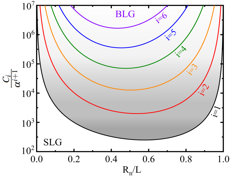
The above discussions are all based on Fig. 5 which is depicts the growth mode on the Cu(111) substrate. An alternative substrate would result in completely different surface kinetics and nucleation preference. Moreover, when the growth temperature varies, not only the values of and change, the border curve also shifts. It is not straightforward to use the current phase diagram to cover these changes. A new diagram may be more helpful in the complicated situation. Fig. 6 shows the phase diagram constructed using and , which is effectively similar to the aforementioned one. Only SLG growth is possible when is sufficiently small. When is larger than the critical value, SLG growth occurs if is extremely large or small. Correspondingly, BLG growth occurs at a moderate value of as increases. Beyond graphene, the phase diagram shown in Fig. 6 can also shed light on the growth control of other 2D materials with IWC growth mode mediated by the expression of and .
VI \@slowromancapvi@. Conclusion
In summary, the mechanism of graphene growth on the Cu substrate is comprehensively studied by a complete analysis of the atomic kinetic processes and the construction of the growth mode diagram. Our diagram identifies the necessary conditions for BLG growth and gives the criteria that distinguish BLG growth from SLG growth. Furthermore, experimental strategies for SLG and BLG growth can be elucidated and summerized using the diagram. Our findings can serve as a guide for new designs of experiments and optimization of experiment parameters, but also inspire other 2D material growth studies with IWC growth mode.
Acknowledgements.
VII acknowledgments
The numerical calculations were carried out at the High Performance Computing Center of Nanjing University. This work was supported by the National Natural Science Foundation of China (Grants No. 12274211).
VIII \@slowromancapvii@. Appendix
VIII.1 A. The saturation concentration of first-layer nuclei
To determine the saturation concentration of first-layer nuclei, we start by assuming nucleation is spontaneous, with only C monomers being mobile on the substrate. The two assumptions presented in the main text are also employed for simplicity. The C monomers arrive at the substrate due to deposition at a rate and diffuse on the substrate with a rate . Adsorbed C monomers may re-desorb and the mean residence time for a monomer is given by , where is the vibrational frequency, is the adsorption energy of a C monomer, is the Boltzmann constant and is the experimental temperature. The remaining C monomers diffuse on the substrate until they encounter other monomers and form dimers. The dimers capture more monomers and grow step-by-step into larger clusters with size . The dimers and clusters also have chance to decay. Clusters of size tend to grow rather than decay. Thus is referred to as the critical nucleus size. All clusters with size larger than are considered stable nuclei.
The concentration of C monomer on the bare substrate far away from any capture zone, , increases due to deposition at the rate and decreases due to re-desorption at rate , formation of C dimer at rate (each dimer removing two monomers), collection into unstable clusters at rate () and stable nuclei at rate . Thus we have
| (12) |
At the steady state , thus the right-hand side of Eq. (12) is equal to zero. When the mean stay time is sufficiently long and the terms and are considerably smaller than the term, the steady value of is determined by the balance between the deposition rate and the capture rate of C monomers by the stable nuclei, , . The capture rate of C monomers by the stable nuclei is given by , where is the average capture number of the stable nuclei and is the concentration of stable nuclei. The steady-state solution of Eq. (12) yields
| (13) |
Note that given in Eq. (13) is the concentration of C monomers far away from the capture zones of stable nuclei. The concentration of C monomer within the capture zones of stable nuclei is much smaller than .
The concentration of stable nuclei, , increases at rate due to new nucleus formation and decreases at rate due to the coalescence of nuclei. The term usually ensures a upper limit for . Here, we consider that the concentration of nuclei reaches saturation before the coalescence of nuclei occurs due to the self-limiting mechanism. In this case we neglect the term and focus on the term only.
Since the C monomer concentration in the near vicinity of the stable nuclei is reduced, nucleation exclusion zones that prohibit nucleation appear exist around stable nuclei and expand as the nuclei grow. The probability of a site being outside nucleation exclusion zones decreases with time exponentially, , , where increases with time in a power lawMarkov (2003). The increasing rate of the stable nuclei concentration is thus as follows
| (14) |
The concentration of critical size nuclei is given by Walton (1962), where is the average binding energy per atom in the first-layer critial nucleus. Combining Eq. (13) , Eq. (14) turns into
| (15) |
The saturation nucleation concentration is obtained by integrating from 0 to as follows
| (16) |
where and is the coverage of first-layer nuclei once its concentration reaches saturation. The half of the first-layer island-island separation is correlated with by relation . Thus the expression of is as follows,
| (17) |
IX B. The nucleation density in experiments
A great deal of researchs have focused on the control of nucleation density in experiments. The nucleation density results and the growth conditions in experiments are listed in Table. LABEL:S1.
| Growth technique | Temperature () | Growth condition | Nucleation density (mm-2) | Nucleation control method | Ref. |
|---|---|---|---|---|---|
| Cu foil APCVD | 1050 | 15 sccm CH4 (500 ppm in Ar) | 0.1 - 1 | foil slightly oxidizing | Gan and Luo (2013) |
| Cu foil APCVD | 950-1080 | 10.5 mTorr CH4 (0.1 in Ar) 19Torr H2 (2.5 in Ar) | 104 - 107 | changing | Vlassiouk et al. (2013) |
| O2-assisted Cu pocket LPCVD | 1035 | (CH4) = 0.001 Torr (H2) = 0.1 Torr | 1 - 103 | O2 exposing time | Hao et al. (2013) |
| Cu foil LPCVD | 950-1050 | 730 sccm CH4 (100 ppm in Ar) 130 sccm H2. (total) = 5 Torr | 104 - 106 | changing | Vlassiouk et al. (2013) |
| Cu foil LPCVD | 950-1050 | 0.3 sccm CH4, 15 sccm H2 (total) = 0.2 Torr | 102 - 103 | changing | Vlassiouk et al. (2013) |
| Cu foil LPCVD | 1070 | H2/CH4 = 1320 (total) = 1-1000 mbar | 103 - 5103 | changing reactor pressure | Zhou et al. (2013) |
| Cu foil LPCVD | 1070 | 0.5 sccm CH4, 10 sccm H2 (total) = 1 Torr | 10 - 103 | foil slightly oxidizing | Eres et al. (2014) |
| Cu foil LPCVD | 1065 | Ar/H2/(0.1)CH4 = 250/26/7 (total) = 50 mbar | 10 - 102 | foil electropolishing | Braeuninger-Weimer et al. (2016) |
| Cu foil LPCVD | 1065 | Ar/H2/(0.1)CH4 = 250/26/7 (total) = 50 mbar | 10-2 - 10 | backside oxidizing | Braeuninger-Weimer et al. (2016) |
| Cu foil LPCVD | 1065 | Ar/H2/(0.1)CH4 = 250/26/7 (total) = 50 mbar | 102 - 104 | foil surface etching | Braeuninger-Weimer et al. (2016) |
| Cu foil LPCVD | 1040 | 5 sccm CH4 20 sccm H2 (total) = 12.5 - 20 Pa | 102 - 104 | changing reactor pressure | Chaitoglou and Bertran (2016) |
| Cu(100) foil LPCVD | 1020 | 1 sccm CH4 20-1700 sccm H2 | 10-6 - 10-2 | changing H2 flow rate | Sun et al. (2016) |
| CuNi alloy APCVD | 1065 | Ar/H2/(0.5)CH4 = 300/15/60-150 (total) = 1 atm | 10-6 - 10-4 | changing CH4 flow rate | Wu et al. (2016) |
| Cu foil APCVD | 1065 | Ar/H2/(0.5)CH4 = 300/15/15-45 (total) = 1 atm | 10-3 - 10-2 | changing CH4 flow rate | Wu et al. (2016) |
| O2-assisted Cu pocket LPCVD | 1060 | 0.3 sccm CH4 (H2) = 10 - 870 Pa | 1 - 10 | changing H2 pressure | Zhao et al. (2016) |
| Cu foil LPCVD | 970-1070 | 5 sccm CH4, 20 sccm H2 (total) = 15 Pa | 102 - 103 | changing | Chaitoglou and Bertran (2017) |
| Cu foil LPCVD | 1040 | Ar/H2/(0.9)CH4 = 320/10/1.6 sccm 0.2 - 4 sccm (0.9)O2 | 10-3 - 10-2 | changing O2 flow rate | Guo et al. (2016) |
| CuNi alloy APCVD | 1075 | Ar/H2/(1)CH4 = 500/50/5 sccm | 1 - 10 | changing Ni content in substrate | Huang et al. (2018) |
| Cu foil LPCVD | 1035-1075 | H2/(0.9)CH4 = 120 (total) = 10 Torr | 10 - 102 | changing | Chan et al. (2018b) |
| CuNi alloy APCVD | 1050 | Ar/H2/(0.5)CH4 = 300/15/60-150 sccm | 10-6 - 10-4 | changing CH4 flow rate | Liu et al. (2018) |
| Co np Cu foil APCVD | 1030 | 1-10 sccm CH4 (22.5-112.5 mTorr) 10 sccm H2 (116.3 mTorr) | 103 - 104 | changing CH4/H2 ratio | Ying et al. (2019) |
References
- Novoselov et al. (2004) K. S. Novoselov, A. K. Geim, S. V. Morozov, D. Jiang, Y. Zhang, S. V. Dubonos, I. V. Grigorieva, and A. A. Firsov, Science 306, 666 (2004).
- Morozov et al. (2008) S. V. Morozov, K. S. Novoselov, M. I. Katsnelson, F. Schedin, D. C. Elias, J. A. Jaszczak, and A. K. Geim, Phys. Rev. Lett. 100, 016602 (2008).
- Lee et al. (2008) C. Lee, X. Wei, J. W. Kysar, and J. Hone, Science 321, 385 (2008).
- Briggs et al. (2010) B. D. Briggs, B. Nagabhirava, G. Rao, R. Geer, H. Gao, Y. Xu, and B. Yu, Appl. Phys. Lett. 97, 223102 (2010).
- Yao et al. (2022a) W. Yao, H. Liu, J. Sun, B. Wu, and Y. Liu, Adv. Funct. Mater. (2022a).
- Cai and Yu (2021) L. Cai and G. Yu, Adv. Mater. 32, 2202584 (2021).
- Bolotin et al. (2008) K. I. Bolotin, K. J. Sikes, Z. Jiang, M. Klima, G. Fudenberg, J. Hone, P. Kim, and H. L. Stormer, Solid State Commun. 146, 351 (2008).
- Nair et al. (2008) R. R. Nair, P. Blake, A. N. Grigorenko, K. S. Novoselov, T. J. Booth, T. Stauber, N. M. R. Peres, and A. K. Geim, Science 320, 1308 (2008).
- Bae et al. (2010) S. Bae, H. Kim, Y. Lee, X. Xu, J.-S. Park, Y. Zheng, J. Balakrishnan, T. Lei, H. Ri Kim, Y. I. Song, Y.-J. Kim, K. S. Kim, B. Özyilmaz, J.-H. Ahn, B. H. Hong, and S. Iijima, Nat. Nanotechnol. 5, 574 (2010).
- Wang et al. (2014) X. Wang, W. Xie, and J.-B. Xu, Adv. Mater. 26, 5496 (2014).
- Xia et al. (2009) F. Xia, T. Mueller, Y.-m. Lin, A. Valdes-Garcia, and P. Avouris, Nat. Nanotechnol. 4, 839 (2009).
- Yu et al. (2015) X. Yu, L. Yang, Q. Lv, M. Xu, H. Chen, and D. Yang, Nanoscale 7, 7072 (2015).
- Zhang et al. (2009) Y. Zhang, T.-T. Tang, C. Girit, Z. Hao, M. C. Martin, A. Zettl, M. F. Crommie, Y. R. Shen, and F. Wang, Nature 459, 820 (2009).
- Mak et al. (2009) K. F. Mak, C. H. Lui, J. Shan, and T. F. Heinz, Phys. Rev. Lett. 102, 256405 (2009).
- Wang et al. (2008) F. Wang, Y. Zhang, C. Tian, C. Girit, A. Zettl, M. Crommie, and Y. R. Shen, Science 320, 206 (2008).
- Yin et al. (2016) J. Yin, H. Wang, H. Peng, Z. Tan, L. Liao, L. Lin, X. Sun, A. L. Koh, Y. Chen, H. Peng, and Z. Liu, Nat. Commun. 7, 10699 (2016).
- Cao et al. (2018a) Y. Cao, V. Fatemi, A. Demir, S. Fang, S. L. Tomarken, J. Y. Luo, J. D. Sanchez-Yamagishi, K. Watanabe, T. Taniguchi, E. Kaxiras, R. C. Ashoori, and P. Jarillo-Herrero, Nature 556, 80 (2018a).
- Cao et al. (2018b) Y. Cao, V. Fatemi, S. Fang, K. Watanabe, T. Taniguchi, E. Kaxiras, and P. Jarillo-Herrero, Nature 556, 43 (2018b).
- Hernandez et al. (2008) Y. Hernandez, V. Nicolosi, M. Lotya, F. M. Blighe, Z. Sun, S. De, I. T. McGovern, B. Holland, M. Byrne, Y. K. Gun’Ko, J. J. Boland, P. Niraj, G. Duesberg, S. Krishnamurthy, R. Goodhue, J. Hutchison, V. Scardaci, A. C. Ferrari, and J. N. Coleman, Nat. Nanotechnol. 3, 563 (2008).
- Shih et al. (2011) C. J. Shih, A. Vijayaraghavan, R. Krishnan, R. Sharma, J. H. Han, M. H. Ham, Z. Jin, S. Lin, G. L. Paulus, N. F. Reuel, Q. H. Wang, D. Blankschtein, and M. S. Strano, Nat. Nanotechnol. 6, 439 (2011).
- Nyakiti et al. (2012) L. O. Nyakiti, R. L. Myers-Ward, V. D. Wheeler, E. A. Imhoff, F. J. Bezares, H. Chun, J. D. Caldwell, A. L. Friedman, B. R. Matis, J. W. Baldwin, P. M. Campbell, J. C. Culbertson, J. Eddy, C. R., G. G. Jernigan, and D. K. Gaskill, Nano Lett. 12, 1749 (2012).
- Virojanadara et al. (2008) C. Virojanadara, M. Syväjarvi, R. Yakimova, L. I. Johansson, A. A. Zakharov, and T. Balasubramanian, Phys. Rev. B 78 (2008).
- Liu et al. (2012a) L. Liu, H. Zhou, R. Cheng, W. J. Yu, Y. Liu, Y. Chen, J. Shaw, X. Zhong, Y. Huang, and X. Duan, ACS Nano 6, 8241 (2012a).
- Seah et al. (2014) C.-M. Seah, S.-P. Chai, and A. R. Mohamed, Carbon 70, 1 (2014).
- López and Mittemeijer (2004) G. A. López and E. J. Mittemeijer, Scr. Mater. 51, 1 (2004).
- Li et al. (2009a) X. Li, W. Cai, L. Colombo, and R. S. Ruoff, Nano Lett. 9, 4268 (2009a).
- Li et al. (2009b) X. Li, W. Cai, J. An, S. Kim, J. Nah, D. Yang, R. Piner, A. Velamakanni, I. Jung, E. Tutuc, S. K. Banerjee, L. Colombo, and R. S. Ruoff, Science 324, 1312 (2009b).
- Edwards and Coleman (2012) R. S. Edwards and K. S. Coleman, Acc. Chem. Res. 46, 23 (2012).
- Li et al. (2009c) M. Li, Y. Han, P. A. Thiel, and J. W. Evans, J. Phys.: Condens. Matter 21, 084216 (2009c).
- Ding et al. (2003) Z. Ding, D. W. Bullock, P. M. Thibado, V. P. LaBella, and K. Mullen, Phys. Rev. Lett. 90, 216109 (2003).
- Nie et al. (2012) S. Nie, W. Wu, S. Xing, Q. Yu, J. Bao, S.-s. Pei, and K. F. McCarty, New J. Phys. 14, 093028 (2012).
- Fang et al. (2013) W. Fang, A. L. Hsu, R. Caudillo, Y. Song, A. G. Birdwell, E. Zakar, M. Kalbac, M. Dubey, T. Palacios, M. S. Dresselhaus, P. T. Araujo, and J. Kong, Nano Lett. 13, 1541 (2013).
- Li et al. (2013) Q. Li, H. Chou, J. H. Zhong, J. Y. Liu, A. Dolocan, J. Zhang, Y. Zhou, R. S. Ruoff, S. Chen, and W. Cai, Nano Lett. 13, 486 (2013).
- Chan et al. (2018a) C.-C. Chan, W.-L. Chung, and W.-Y. Woon, Carbon 135, 118 (2018a).
- Wu et al. (2010) P. Wu, W. Zhang, Z. Li, J. Yang, and J. G. Hou, J. Chem. Phys. 133, 071101 (2010).
- Li et al. (2017) P. Li, Z. Li, and J. Yang, J. Phys. Chem. C 121, 25949 (2017).
- Gao et al. (2011a) J. Gao, J. Yip, J. Zhao, B. I. Yakobson, and F. Ding, J. Am. Chem. Soc. 133, 5009 (2011a).
- Gao et al. (2011b) J. Gao, Q. Yuan, H. Hu, J. Zhao, and F. Ding, J. Phys. Chem. C 115, 17695 (2011b).
- Kim et al. (2012) H. Kim, C. Mattevi, M. R. Calvo, J. C. Oberg, L. Artiglia, S. Agnoli, C. F. Hirjibehedin, M. Chhowalla, and E. Saiz, ACS Nano 6, 3614 (2012).
- Chen et al. (2015) W. Chen, P. Cui, W. Zhu, E. Kaxiras, Y. Gao, and Z. Zhang, Phys. Rev. B 91 (2015).
- Chen et al. (2010) H. Chen, W. Zhu, and Z. Zhang, Phys. Rev. Lett. 104, 186101 (2010).
- Riikonen et al. (2012) S. Riikonen, A. V. Krasheninnikov, L. Halonen, and R. M. Nieminen, J. Phys. Chem. C 116, 5802 (2012).
- Wu et al. (2015) P. Wu, Y. Zhang, P. Cui, Z. Li, J. Yang, and Z. Zhang, Phys. Rev. Lett. 114, 216102 (2015).
- Andersen et al. (2019) M. Andersen, J. S. Cingolani, and K. Reuter, J. Phys. Chem. C 123, 22299 (2019).
- Zhang et al. (2014) X. Zhang, L. Wang, J. Xin, B. I. Yakobson, and F. Ding, J. Am. Chem. Soc. 136, 3040 (2014).
- Kresse and Furthmüller (1996a) G. Kresse and J. Furthmüller, Comput. Mater. Sci 6, 15 (1996a).
- Kresse and Furthmüller (1996b) G. Kresse and J. Furthmüller, Phys. Rev. B 54, 11169 (1996b).
- Perdew et al. (1996) J. P. Perdew, K. Burke, and M. Ernzerhof, Phys. Rev. Lett. 77, 3865 (1996).
- Blochl (1994) P. E. Blochl, Phys. Rev. B 50, 17953 (1994).
- Bučko et al. (2010) T. Bučko, J. Hafner, S. Lebẽgue, and J. G. Ángyán, J. Phys. Chem. A 114, 11814 (2010).
- Methfessel and Paxton (1989) M. Methfessel and A. T. Paxton, Phys. Rev. B 40, 3616 (1989).
- Henkelman et al. (2000) G. Henkelman, B. P. Uberuaga, and H. Jónsson, J. Chem. Phys. 113, 9901 (2000).
- Zhong et al. (2016) L. Zhong, J. Li, Y. Li, H. Lu, H. Du, L. Gan, C. Xu, S. W. Chiang, and F. Kang, J. Phys. Chem. C 120, 23239 (2016).
- Wu et al. (2014) P. Wu, X. Zhai, Z. Li, and J. Yang, J. Phys. Chem. C 118, 6201 (2014).
- Hao et al. (2013) Y. Hao, M. S. Bharathi, L. Wang, Y. Liu, H. Chen, S. Nie, X. Wang, H. Chou, C. Tan, B. Fallahazad, H. Ramanarayan, C. W. Magnuson, E. Tutuc, B. I. Yakobson, K. F. McCarty, Y.-W. Zhang, P. Kim, J. Hone, L. Colombo, and R. S. Ruoff, Science 342, 720 (2013).
- Venables (1973) J. A. Venables, Philos. Mag. 27, 697 (1973).
- Venables et al. (1984) J. A. Venables, G. D. T. Spiller, and M. Hanbucken, Rep. Prog. Phys. 47, 399 (1984).
- Zhao et al. (2016) P. Zhao, Y. Cheng, D. Zhao, K. Yin, X. Zhang, M. Song, S. Yin, Y. Song, P. Wang, M. Wang, Y. Xia, and H. Wang, Nanoscale 8, 7646 (2016).
- Walton (1962) D. Walton, J. Chem. Phys. 37, 2182 (1962).
- Shu et al. (2017) D.-J. Shu, X. Xiong, M. Liu, and M. Wang, Phys. Rev. B 96 (2017).
- Li et al. (2010) X. Li, C. W. Magnuson, A. Venugopal, J. An, J. W. Suk, B. Han, M. Borysiak, W. Cai, A. Velamakanni, Y. Zhu, L. Fu, E. M. Vogel, E. Voelkl, L. Colombo, and R. S. Ruoff, Nano Lett. 10, 4328 (2010).
- Chan et al. (2013) S.-H. Chan, S.-H. Chen, W.-T. Lin, M.-C. Li, Y.-C. Lin, and C.-C. Kuo, Nanoscale Res. Lett. 8, 285 (2013).
- Chaitoglou and Bertran (2016) S. Chaitoglou and E. Bertran, Mater. Res. Express 3, 075603 (2016).
- Sun et al. (2016) L. Sun, L. Lin, J. Zhang, H. Wang, H. Peng, and Z. Liu, Nano Res. 10, 355 (2016).
- Wu et al. (2016) T. Wu, X. Zhang, Q. Yuan, J. Xue, G. Lu, Z. Liu, H. Wang, H. Wang, F. Ding, Q. Yu, X. Xie, and M. Jiang, Nat. Mater. 15, 43 (2016).
- Zhou et al. (2013) H. Zhou, W. J. Yu, L. Liu, R. Cheng, Y. Chen, X. Huang, Y. Liu, Y. Wang, Y. Huang, and X. Duan, Nat. Commun. 4, 2096 (2013).
- Guo et al. (2016) W. Guo, F. Jing, J. Xiao, C. Zhou, Y. Lin, and S. Wang, Adv. Mater. 28, 3152 (2016).
- Chen et al. (2012) W. Chen, H. Chen, H. Lan, P. Cui, T. P. Schulze, W. Zhu, and Z. Zhang, Phys. Rev. Lett. 109, 265507 (2012).
- Shi et al. (2021) H. Shi, Y. Guo, Z. Qi, K. Xie, R. Zhang, Y. Xia, C. Chen, H. Zeng, P. Cui, H. Ji, S. Qin, and Z. Zhang, J. Phys. Chem. C 125, 18217 (2021).
- Luo et al. (2017) B. Luo, J. M. Caridad, A. G. Čabo, P. Bøggild, P. R. Whelan, S. K. Mahatha, and T. J. Booth, 2D Mater. 4, 045017 (2017).
- Nguyen et al. (2019) D. T. Nguyen, W. Y. Chiang, Y. H. Su, M. Hofmann, and Y. P. Hsieh, Sci. Rep. 9, 257 (2019).
- Luo et al. (2019) D. Luo, M. Wang, Y. Li, C. Kim, K. M. Yu, Y. Kim, H. Han, M. Biswal, M. Huang, Y. Kwon, M. Goo, D. C. Camacho-Mojica, H. Shi, W. J. Yoo, M. S. Altman, H.-J. Shin, and R. S. Ruoff, Adv. Mater. 31, 1903615 (2019).
- Yao et al. (2022b) W. Yao, J. Zhang, J. Ji, H. Yang, B. Zhou, X. Chen, P. Bøggild, P. U. Jepsen, J. Tang, F. Wang, L. Zhang, J. Liu, B. Wu, J. Dong, and Y. Liu, Adv. Mater. 34, 2108608 (2022b).
- Braeuninger-Weimer et al. (2016) P. Braeuninger-Weimer, B. Brennan, A. J. Pollard, and S. Hofmann, Chem. Mater. 28, 8905 (2016).
- Huang et al. (2018) M. Huang, M. Biswal, H. J. Park, S. Jin, D. Qu, S. Hong, Z. Zhu, L. Qiu, D. Luo, X. Liu, Z. Yang, Z. Liu, Y. Huang, H. Lim, W. J. Yoo, F. Ding, Y. Wang, Z. Lee, and R. S. Ruoff, ACS Nano 12, 6117 (2018).
- Liu et al. (2018) Y. Liu, T. Wu, Y. Yin, X. Zhang, Q. Yu, D. J. Searles, F. Ding, Q. Yuan, and X. Xie, Adv. Sci. 5, 1700961 (2018).
- Sun et al. (2021a) L. Sun, B. Chen, W. Wang, Y. Li, X. Zeng, H. Liu, Y. Liang, Z. Zhao, A. Cai, R. Zhang, Y. Zhu, Y. Wang, Y. Song, Q. Ding, X. Gao, H. Peng, Z. Li, L. Lin, and Z. Liu, ACS Nano 16, 285 (2021a).
- Srinivasan et al. (2018) B. M. Srinivasan, Y. Hao, R. Hariharaputran, S. Rywkin, J. C. Hone, L. Colombo, R. S. Ruoff, and Y. W. Zhang, ACS Nano 12, 9372 (2018).
- Gan and Luo (2013) L. Gan and Z. Luo, ACS Nano 7, 9480 (2013).
- Eres et al. (2014) G. Eres, M. Regmi, C. M. Rouleau, J. Chen, I. N. Ivanov, A. A. Puretzky, and D. B. Geohegan, ACS Nano 8, 5657–5669 (2014).
- Lim et al. (2020) H. Lim, H. C. Lee, M. S. Yoo, A. Cho, N. N. Nguyen, J. W. Han, and K. Cho, Chem. Mater. 32, 10357 (2020).
- Sun et al. (2021b) L. Sun, Z. Wang, Y. Wang, L. Zhao, Y. Li, B. Chen, S. Huang, S. Zhang, W. Wang, D. Pei, H. Fang, S. Zhong, H. Liu, J. Zhang, L. Tong, Y. Chen, Z. Li, M. H. Rummeli, K. S. Novoselov, H. Peng, L. Lin, and Z. Liu, Nat. Commun. 12, 2391 (2021b).
- Ying et al. (2019) H. Ying, W. Wang, W. Liu, L. Wang, and S. Chen, Carbon 146, 549 (2019).
- Huang et al. (2020) M. Huang, P. V. Bakharev, Z. J. Wang, M. Biswal, Z. Yang, S. Jin, B. Wang, H. J. Park, Y. Li, D. Qu, Y. Kwon, X. Chen, S. H. Lee, M. G. Willinger, W. J. Yoo, Z. Lee, and R. S. Ruoff, Nat. Nanotechnol. 15, 289 (2020).
- Liu et al. (2019) B. Liu, Y. Sheng, S. Huang, Z. Guo, K. Ba, H. Yan, W. Bao, and Z. Sun, Chem. Mater. 31, 6105 (2019).
- Hao et al. (2016) Y. Hao, L. Wang, Y. Liu, H. Chen, X. Wang, C. Tan, S. Nie, J. W. Suk, T. Jiang, T. Liang, J. Xiao, W. Ye, C. R. Dean, B. I. Yakobson, K. F. McCarty, P. Kim, J. Hone, L. Colombo, and R. S. Ruoff, Nat. Nanotechnol. 11, 426 (2016).
- Yan et al. (2011) K. Yan, H. Peng, Y. Zhou, H. Li, and Z. Liu, Nano Lett 11, 1106 (2011).
- Liu et al. (2012b) L. Liu, H. Zhou, R. Cheng, W. J. Yu, Y. Liu, Y. Chen, J. Shaw, X. Zhong, Y. Huang, and X. Duan, ACS Nano 6, 8241 (2012b).
- Qi et al. (2018) Z. Qi, H. Shi, M. Zhao, H. Jin, S. Jin, X. Kong, R. S. Ruoff, S. Qin, J. Xue, and H. Ji, Chem. Mater. 30, 7852 (2018).
- Markov (2003) I. V. Markov, Crystal Growth for Beginners, 2nd ed. (World Scientific, Singapore, 2003).
- Vlassiouk et al. (2013) I. Vlassiouk, S. Smirnov, M. Regmi, S. P. Surwade, N. Srivastava, R. Feenstra, G. Eres, C. Parish, N. Lavrik, P. Datskos, S. Dai, and P. Fulvio, J. Phys. Chem. C 117, 18919 (2013).
- Chaitoglou and Bertran (2017) S. Chaitoglou and E. Bertran, J. Mater. Sci. 52, 8348 (2017).
- Chan et al. (2018b) C.-C. Chan, W.-L. Chung, and W.-Y. Woon, Carbon 135, 118 (2018b).