EEG-ImageNet: An Electroencephalogram Dataset and Benchmarks with Image Visual Stimuli of Multi-Granularity Labels

Abstract

Identifying and reconstructing what we see from brain activity gives us a special insight into investigating how the biological visual system represents the world. While recent efforts have achieved high-performance image classification and high-quality image reconstruction from brain signals collected by Functional Magnetic Resonance Imaging (fMRI) or magnetoencephalogram (MEG), the expensiveness and bulkiness of these devices make relevant applications difficult to generalize to practical applications. On the other hand, Electroencephalography (EEG), despite its advantages of ease of use, cost-efficiency, high temporal resolution, and non-invasive nature, has not been fully explored in relevant studies due to the lack of comprehensive datasets. To address this gap, we introduce EEG-ImageNet, a novel EEG dataset comprising recordings from 16 subjects exposed to 4000 images selected from the ImageNet dataset. EEG-ImageNet consists of 5 times EEG-image pairs larger than existing similar EEG benchmarks. EEG-ImageNet is collected with image stimuli of multi-granularity labels, i.e., 40 images with coarse-grained labels and 40 with fine-grained labels. Based on it, we establish benchmarks for object classification and image reconstruction. Experiments with several commonly used models show that the best models can achieve object classification with accuracy around 60% and image reconstruction with two-way identification around 64%. These results demonstrate the dataset’s potential to advance EEG-based visual brain-computer interfaces, understand the visual perception of biological systems, and provide potential applications in improving machine visual models.

1 Introduction

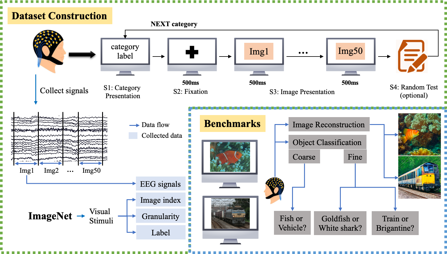
Figure 1: The overall procedure of our dataset construction and benchmark design.

Recent advancements in reconstructing visual experiences from the human brain have seen significant progress, largely driven by the extensive use of functional magnetic resonance imaging (fMRI) ([8, 22, 23]) and magnetoencephalogram (MEG) [3] datasets. fMRI and MEG are widely used to investigate various cognitive functions, neurological disorders, and brain connectivity patterns ([2, 40, 37, 35]). Driven by the use of deep neural networks, particularly diffusion-based and transformer-based models( [34, 30, 25, 6]), it is even possible to reconstruct human’s visual perceptions from fMRI or MEG recordings. The application of large-scale deep neural networks in neuroscience research has further underscored the importance of large-scale and high-quality datasets [27, 20]. For example, the Natural Scenes Dataset ([1]), contains up to hundreds of thousands of high-quality natural image-fMRI pairs of 8 subjects, providing a solid data foundation for recent work in visual neuroscience. These models and large-scale datasets, in turn, have opened new avenues for understanding the brain’s intricate functions and for developing advanced applications in brain-computer interfaces, neuroimaging, and beyond [33].

On the other hand, electroencephalography (EEG) is another vital tool in neuroscience research. In comparison with fMRI and MEG, EEG is easy to use, cost-efficient, and has superior temporal resolution, making it a valuable tool for capturing rapid and real-time brain dynamics on the order of milliseconds [36]. EEG signals can be obtained non-invasively by placing electrodes on the scalp, making it a less intrusive method for monitoring brain activity. These attributes position EEG as another promising modality for visual neuroscience research.

Although visual reconstruction has been achieved using fMRI and MEG, the high cost and inconvenience of these devices limit their widespread application in practical settings. In contrast, EEG presents advantages over both fMRI and MEG with its cost-efficient and portable features. However, studies on visual perception with EEG signals are limited because of two challenges: (1) the lack of large-scale, high-quality EEG datasets and (2) existing EEG datasets typically featured coarse-grained image categories, lacking fine-grained categories. To the best of our knowledge, the most frequently used dataset is the data set provided by Spampinato et al. [32], which involves 6 participants each watching 2000 image stimuli. However, this dataset’s scale is smaller than existing fMRI datasets, limiting the possibilities for investigating neural aspects related to visual perception and developing deep learning models for relevant visual classification and reconstruction tasks.

On the other hand, the labels in existing EEG datasets are frequently coarse and lack the granularity needed for detailed analysis. Multi-granularity labels are essential because they allow for a more nuanced analysis at different levels of detail. For instance, labels can range from broad categories like “panda” or “golf ball” to more specific attributes like “Rottweiler” or “Samoyed”. These challenges underscore the necessity for new, large-scale EEG datasets with high-quality, multi-granularity labels. Such datasets would enable researchers to explore the intricacies of visual processing with greater accuracy and depth, facilitating advancements in both basic neuroscience and applied fields like brain-computer interfaces and clinical diagnostics.

To address these challenges, we present EEG-ImageNet, a novel EEG dataset specifically designed to promote research related to visual neuroscience, biomedical engineering, etc. EEG-ImageNet is a comprehensive dataset that includes EEG recordings from 16 subjects, each exposed to 4,000 images sourced from the ImageNet-21k [28]. These images span 80 different categories, with 50 images per category. The dataset is structured to support multi-granularity analysis, with 40 categories dedicated to coarse-grained tasks and 40 to fine-grained tasks. This dataset aims to bridge the gap in the current research landscape by providing a resource that leverages the strengths of EEG and supports diverse research needs. To demonstrate the utility of this dataset, we establish benchmarks for two primary tasks: object classification and image reconstruction. For the object classification task, we evaluated the dataset using several commonly used models, achieving a best accuracy of 60.88% on the 80-class classification. In the image reconstruction task, our experiments with advanced generative models produced promising results, with the best model achieving a two-way identification of 64.67%. These benchmarks demonstrate the dataset’s potential for advancing EEG-based research. Figure 1 shows the overall procedure of our dataset construction and benchmark design. By addressing the lack of large-scale, high-quality EEG datasets, EEG-ImageNet aims to drive EEG-based visual research forward, improve machine learning models, and provide deeper insights into visual perception and processing.

2 Related Work

In this section, we review some datasets related to visual recognition and neuroscience and compare them with EEG-ImageNet, as shown in Table 1.

2.1 Visual Recognition Dataset

Visual recognition is a cornerstone of computer vision, driven by datasets like ImageNet [28], CIFAR [16], and MS COCO [20]. ImageNet contains over 14 million annotated images, CIFAR-10/100 consist of thousands of 32x32 images in 10 and 100 classes, respectively, and MS COCO is known for its rich annotations supporting tasks such as object detection and segmentation. Later works have matched image datasets with additional modalities.

Efforts to combine visual recognition with neuroscience have led to datasets like the Microsoft COCO Captions [5], which adds textual descriptions to the MS COCO images, enhancing the dataset with a multimodal aspect for evaluating image captioning models. The SALICON dataset [10] extends MS COCO with eye-tracking data, enabling the study of visual attention and saliency through large-scale annotations. Neuroscience datasets utilizing fMRI have further enriched this field. The BOLD5000 dataset [4] includes fMRI data from subjects viewing 5000 images, aiding the exploration of visual perception. The Generic Object Decoding dataset [9] captures brain activity while subjects view and imagine objects, facilitating the decoding of mental images. The VIM-1 dataset [14] from the study “Identifying Natural Images from Human Brain Activity” demonstrates the feasibility of decoding viewed images from brain activity. Additionally, the NSD [1] is a large-scale fMRI dataset in visual neuroscience, recording high-resolution (1.8-mm) whole-brain 7T fMRI data from eight subjects exposed to 9,000–10,000 color natural scenes from the MS COCO dataset over the course of a year. Integrating neuroimaging and eye-tracking datasets with visual recognition tasks has opened new avenues for understanding how the brain interprets visual information, leading to insights and applications in brain-computer interfaces and neural decoding.

Table 1: Detailed metadata for various neurological datasets based on visual stimuli.

Dataset	#Subjects	Modalities	Visual Stimuli	#Stimuli	#Stimuli per Subject
SALICON [10]	-	Eye-tracking	MS COCO [20]	20,000	-
BOLD5000 [4]	4	fMRI	ImageNet [28], MS COCO, SceneUN [38]	5,254	1,157-1,798
GOD [9]	5	fMRI	ImageNet	1,200	1,200
VIM-1 [14]	2	fMRI	Corel Stock Photo Library [11]	1,870	1,870
NSD [1]	8	fMRI, Eye-tracking	MS COCO	9,000-10,000	22,000–30,000
Spampinato et al. [32]	6	EEG	ImageNet	2000	2000
EEG-SVRec [42]	30	EEG, ECG	short videos	2636	121.9
EEG-ImageNet	16	EEG	ImageNet	4,000	4,000

• Note: The original SALICON dataset lacks information on the number of subjects involved.

2.2 EEG dataset

fMRI is renowned for its high spatial resolution, allowing researchers to obtain detailed images of brain activity by measuring changes in blood flow [23]. In contrast, EEG offers several distinct advantages over fMRI. EEG is relatively easy to use and cost-efficient, with a straightforward setup that involves placing electrodes on the scalp to measure electrical activity. One of the most significant benefits of EEG is its exceptional temporal resolution, which captures neural dynamics on the order of milliseconds [36]. This high temporal resolution makes EEG ideal for studying fast-occurring brain processes and real-time neural responses, providing insights into the timing and sequence of neural events [21]. EEG’s non-invasive nature also makes it suitable for a wider range of participants. However, EEG signals collected using portable devices often have a low signal-to-noise ratio, which can complicate data analysis and reduce the accuracy of the results [13].

Existing EEG datasets span a variety of research areas. The SEED [43] focuses on emotion recognition with detailed EEG recordings from subjects exposed to various emotional stimuli. The BCI Competition IV datasets [41] provide EEG data for motor imagery tasks, while the TUH EEG Corpus [31] is a large clinical EEG collection often used for benchmarking EEG data quality across different conditions. The DEAP [15] collects EEG and peripheral physiological signals from 32 participants as they watch 40 one-minute music videos, providing comprehensive emotional responses. Similarly, the AMIGOS [24] captures EEG and physiological responses from participants watching short video clips designed to evoke specific emotional states. In the realm of visual recognition, datasets like the EEG-Classification dataset [32] involve 6 subjects viewing 2,000 images across 40 object classes from the ImageNet10k. Another significant dataset is the EEG-SVRec [42], which includes EEG recordings from 30 participants interacting with short videos, aiming to capture detailed affective experiences.

In comparison, the EEG-ImageNet dataset offers several advantages. Firstly, its larger scale is conducive to training deep learning models. Secondly, the greater number of subjects facilitates inter-subject experiments and analyses. Additionally, the dataset features multi-granularity image labels, and the images are of high quality, selected from ImageNet21k and filtered to exclude small, blurry, or watermarked pictures.

3 Dataset Construction

During the data collection process of our user study, participants are presented with a visual stimuli dataset containing 4000 natural images from ImageNet. Throughout this process, we continuously record their EEG signals. The whole experimental process is carried out in the laboratory environment. This section describes the entire process of EEG-ImageNet dataset construction. The EEG-ImageNet dataset can be accessed openly through the url https://github.com/Promise-Z5Q2SQ/EEG-ImageNet-Dataset.

3.1 Ethical and Privacy

To protect participants’ privacy and physical health, our user study adheres to strict ethical guidelines for human research, with approval from the ethics committee of the School of Psychology at Tsinghua University. The study has undergone a comprehensive ethical review to safeguard participants’ rights. In accordance with ethical standards, we have taken several steps to protect participants’ privacy, including data anonymization and obtaining informed consent from all participants. Additionally, participants are thoroughly informed about the study’s objectives, procedures, and potential outcomes. The EEG data collection method employed in this research is non-invasive and poses no risk to participants. This approach ensures compliance with ethical standards while maintaining the integrity of the research findings.

3.2 Participants

We enlist a total of 16 participants via social media, including 10 males and 6 females. These participants are all college students aged between 21 and 27, with an average age of 24.06 and a standard deviation of 1.69. Their majors encompass computer science, mechanical engineering, chemistry, and environmental engineering, and they range from undergraduate to postgraduate levels. All participants are right-handed and assert their proficiency in utilizing image search engines in their daily routines. Each participant dedicates approximately 2 hours to complete the experiment, which includes 30 minutes for equipment setup and task instructions. Before the experiment, participants are informed of a compensation of US$11.8 per hour upon completion, to ensure the quality of the data collected for the study.

3.3 Stimuli Dataset

The dataset used for visual stimuli was a subset of ImageNet21k, containing 80 categories of objects. Each category comprises 50 manually curated images, ensuring that each image has a width and height greater than 300 pixels and prominently features an object corresponding to its class label in ImageNet. Additionally, every image is free of watermarks. In this manner, we have selected a total of 4000 high-quality natural images as our visual stimulus dataset.

Among all categories, the first half is consistent with the EEG-Classification dataset ([32]), comprising 40 significantly distinct categories from ImageNet1k. We treat these as coarse-grained tasks. The latter 40 categories are designed as a fine-grained task, divided into 5 groups with 8 categories each. The categories within the same group share the same parent node in WordNet, and each category label is either a leaf node or a sub-leaf node in WordNet. This selection ensures that the chosen categories represent similar granularity while avoiding overly obscure categories, thereby minimizing potential biases in the experimental results. For instance, coarse-grained categories include items such as African elephants, pandas, mobile phones, golf balls, bananas, and pizzas. Under the parent node "musical instruments," the fine-grained categories include accordions, cellos, flutes, oboes, snare drums, and trombones. Detailed information about all the visual stimuli categories and their respective WordNet IDs can be found in our GitHub repository.

3.4 Procedure

Before engaging in the user study, participants are required to fill out an entry questionnaire and sign a consent about the protection of privacy security. They will receive an orientation regarding the primary tasks and operational procedures. Additionally, they will be notified of their right to withdraw from the study at any point. Before the main trials, participants will undergo a series of training trials designed to acquaint participants with the procedures of the formal experiments.

Every participant is required to select a random seed before the experiment to randomize the order of the categories. This randomization guarantees a fair distribution of categories and images among participants. The experimental platform follows a sequential and repetitive process as illustrated in Figure 1. (S1) The experimental platform presents the current category label. Participants can proceed to the next stage by pressing the space key. (S2) A fixation cross is shown at the center of the screen, ensuring attention is drawn when images are displayed. This fixation period lasts for 500 ms. (S3) The 50 images of this category are sequentially presented using the Rapid Serial Visual Presentation (RSVP) paradigm, which is commonly employed in psychological experiments. Each image is presented for a duration of 500 ms [12]. (S4) Random tests are conducted to verify the participant’s engagement in the experiment after the presentation. Data from categories for which participants fail the test will not be included in final analyses. The EEG signals of the participant will be captured and recorded continuously during the entire process. The program will cycle back to step S1 and display the next category, repeating this process until all the images have been presented.

3.5 Dataset Description

The EEG-ImageNet dataset contains a total of 63,850 EEG-image pairs from 16 participants. Each EEG data sample has a size of (n_channels, $f_{s}\cdot T$), where n_channels is the number of EEG electrodes, which is 62 in our dataset; $f_{s}$ is the sampling frequency of the device, which is 1000 Hz in our dataset; and T is the time window size, which in our dataset is the duration of the image stimulus presentation, i.e., 0.5 seconds. Due to ImageNet’s copyright restrictions, our dataset only provides the file index of each image in ImageNet and the wnid of its category corresponding to each EEG segment. Additional information about the dataset is shown in Appendix A.1.

4 Benchmarks

In this section, we detail the benchmarks of our study shown in Figure 1 by outlining the preprocessing steps, feature extraction methods, task definitions, and models used.

4.1 Preprocessing

We perform a series of preprocessing steps for the raw EEG data we collect to eliminate noise and artifacts and improve signal quality. The preprocessing pipeline includes the following stages: First, re-referencing: Re-referencing is done using the offline linked mastoids method, which uses the average of the M1 and M2 mastoid electrodes as the new reference point [39]. This minimizes potential biases and improves the signal-to-noise ratio. Then, filtering: Filtering is performed using a 0.5 Hz to 80 Hz band-pass filter to remove low-frequency drifts (<0.5 Hz) and high-frequency noise (>80 Hz). Additionally, 50 Hz environmental noise is eliminated. Finally, artifact removal: Artifact removal eliminates abnormal amplitude signals and artifacts caused by blinks or head movements.

4.2 Feature Extraction

In our benchmarks, for models requiring time-domain signals as direct input, we extract the 40ms-440ms segment of each EEG signal as the feature input. This approach helps to minimize the influence of preceding and subsequent image stimuli on the current stimulus. For models requiring frequency-domain features as input, we extract the differential entropy (DE) of the extracted time-domain signals as features, as this characteristic effectively captures the complexity and variability of brain activity in the frequency domain [7]. According to the general division in neuroscience, the frequency bands are categorized as delta (0.5-4 Hz), theta (4-8 Hz), alpha (8-13 Hz), beta (13-30 Hz), and gamma (30-80 Hz). We use the Welch method with a sliding window to estimate the power spectral density $P(f)$ in each frequency band. Then, we normalize the data and calculate the differential entropy (DE) using the formula, $DE=-\int P(f)\log(P(f))df$. Consequently, for each segment of EEG signals, we obtain the differential entropy (DE) for each electrode and each frequency band.

4.3 Task Definition

In our benchmarks, we test our dataset on two tasks: object classification and image reconstruction. The object classification task aims to classify the category of the corresponding image stimulus the participant is exposed to with their EEG signals. We evaluate the models using classification accuracy. In the image reconstruction task, given a specific EEG segment, the goal is to reconstruct the image stimulus the participant is exposed to. We evaluate the generated results using two-way identification [30] under different visual neural networks (refer to Appendix A.3 for details.).

On our multi-granularity labeled image dataset, we test various tasks with different levels of granularity. Additionally, due to the inherent significant inter-individual differences in EEG signals, all models in our benchmarks are trained exclusively in an intra-subject experimental setup. Furthermore, to mitigate the significant temporal effects [19] observed in the EEG-Classification dataset, all our experimental setups strictly adhere to a dataset split where the first 30 images of each category are used as the training set, and the last 20 images are used as the test set. We strongly recommend that all researchers using the EEG-ImageNet dataset adopt a similar dataset split methodology. We also explain the impact of this split in Appendix A.5.

4.4 Models

In the object classification task, we employ simple machine-learning classification models such as ridge regression, KNN, random forest, and SVM. Additionally, we implement deep learning models including MLP, EEGNet [17], and RGNN [44]. MLP consists of two hidden layers, while EEGNet and RGNN are implemented using their original architectures. We use cross-entropy as the loss function. We train the models for each participant for 2000-3000 epochs on an NVIDIA 4090 GPU.

In the image reconstruction task, we use a frozen Stable Diffusion 1.4 [29] as the backbone and train a two-layer MLP as an encoder to generate the prompt embeddings for input. For our reconstructions, we use 50 denoising timesteps with PNDM noise scheduling to generate 512x512 images. We use MSE as the loss function to align the encoder’s output with the CLIP (ViT-L/14) [26] embeddings of the captions of real images obtained through BLIP [18]. The model for each participant is trained for 2000 epochs with on an NVIDIA 4090 GPU.

For model and training details, please refer to the open-source code and Appendix A.3.

5 Experiments

In this chapter, we present the experimental results of our study, focusing on two benchmark tasks: object classification and image reconstruction.

5.1 Object Classification

In the object classification task, we conduct experiments at three levels of granularity: all, coarse, and fine. The “all” category represents the 80-class classification accuracy, the “coarse” category represents the 40-class classification accuracy, and the “fine” category represents the average accuracy of five 8-class classification tasks. The performance of each model is detailed in Table 2, which shows the average results of all participants.

Table 2: The average results of all participants in the object classification task. * indicates the use of time-domain features, otherwise it indicates the use of frequency-domain features. † indicates that the difference compared to the best-performing model is significant with p-value < 0.05.

Model		Acc (all)	Acc (coarse)	Acc (fine)
Classic model	Ridge	0.2859†	0.3944†	0.5833†
	KNN	0.3037†	0.4012†	0.6954†
	RandomForest	0.3489†	0.4535†	0.7288†
	SVM	0.3919	0.5057†	0.7784†
Deep model	MLP	0.4037	0.5339	0.8163
	EEGNet*	0.2604†	0.3030†	0.3645†
	RGNN	0.4050	0.4703†	0.7057†

The table shows that RGNN achieves the highest accuracy in the “all” task among all models, with an 80-class classification accuracy reaching 40.50%. MLP slightly lags behind RGNN in the “all” task accuracy, but it significantly outperforms in the “coarse” and “fine” tasks, with a 40-class accuracy of 53.39% and an average 8-class accuracy of 81.63%. Among the classical machine learning models, SVM exhibits the highest classification performance, only slightly trailing RGNN and MLP across the three different granularity scenarios. The lower accuracy of RGNN in the “fine” task might be due to the complex model structure, which may require more fine-tuning to better adapt to easier tasks. Meanwhile, the lower performance of time-domain features compared to frequency-domain features suggests that frequency-domain features might be more informative for the classification tasks in this study. Specific performance details for each participant in each task are provided in Appendix A.4. We find that the ranking of participants’ accuracy is relatively consistent across different models.

We compile the accuracy of each participant for the “all” task under the SVM, MLP, and RGNN models, as shown in Figure 2(a). We observe significant differences between participants, indicating high variability in individual responses. The best-performing participant achieves an accuracy of 60.88%. To better compare the differences between “fine” and “coarse” tasks in EEG-ImageNet, we modify the coarse-grained task. We randomly select 8 coarse-grained categories and use the RGNN model for training and testing. This process is repeated 5 times, and the average accuracy for each participant is calculated and plotted alongside their average “fine” task accuracy in Figure 2(b). We then perform linear regression on the data points, and the resulting function has a slope greater than 1, indicating that participants generally achieve better results on the “coarse” classification tasks. This finding is also consistent with intuition.

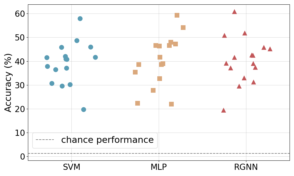
(a) Classfication accuracy for each participant in the object classification task (all) across different Models.

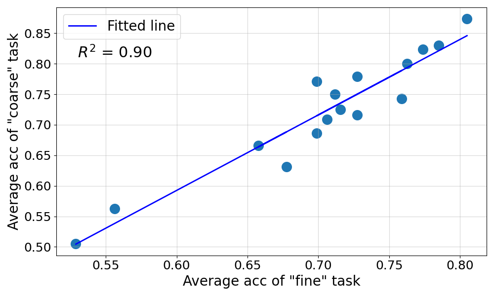
(b) Classification accuracy of the “coarse” (vertical axis) and “fine” task (horizontal axis)).

Figure 2: Classification performance of the object classification, each dot represents the classification performance of a single participant.

5.2 Image Reconstruction

Figure 3 shows some of the results from our image reconstruction pipeline of a single participant (S8). From the selected images, it can be seen that the reconstruction pipeline can effectively restore the category information of the image stimuli. However, restoring low-level details such as color, position, and shape is inaccurate. This may be because we align the EEG signals to the image captions obtained from BLIP. Due to the limited descriptive precision of BLIP, we cannot fully leverage the diffusion model’s generative capabilities.

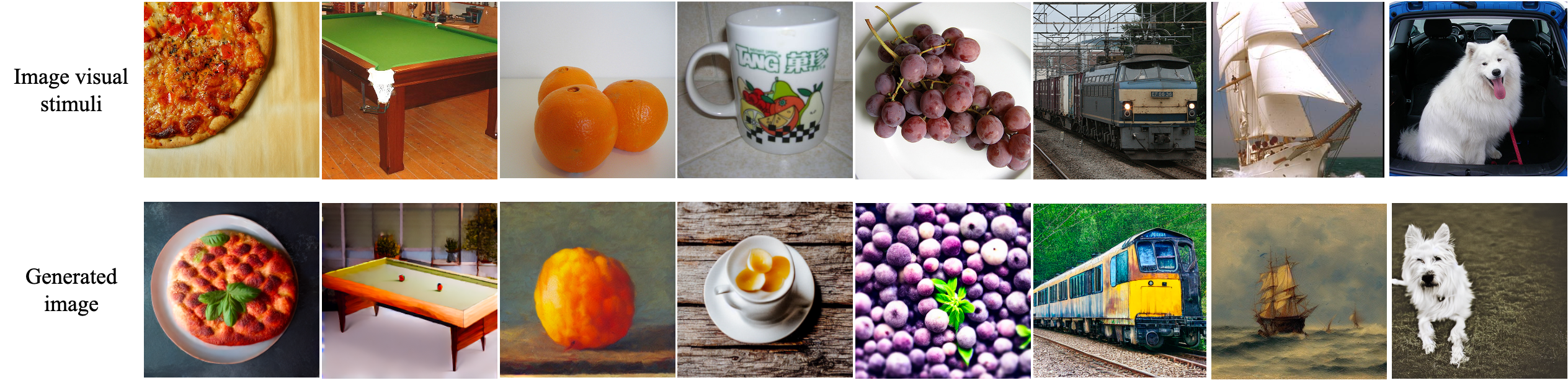
Figure 3: The image reconstruction results of a single participant (S8).

Table 3 shows the average two-way identification (chance=50%) of the images generated by our reconstruction pipeline using different visual neural networks. Two-way identification refers to comparing the generated image with the original and one distractor to evaluate accuracy. The highest accuracy achieved by CLIP suggests that integrating vision transformers with extensive pre-training on diverse image-text data can significantly enhance model performance for complex tasks like image reconstruction from EEG signals. Additional results can be found in Appendix A.4.

Table 3: The average results of all participants in the image reconstruction task.

Method	Alex(2)	Alex(5)	Incep	CLIP(ViT-L/14)
Two-way Identification	56.05%	62.99%	56.75%	64.67%

6 Discussion and Conclusion

In this section, we outline the limitations of our dataset and explore how it could guide future research efforts to advance machine learning and brain-computer interface design.

Limitation. Firstly, while our dataset is more comprehensive than similar works, each participant’s data is still relatively limited. This necessitates the development of inter-subject models to overcome this limitation and enhance generalizability. Additionally, it is limited in representation, as participants were drawn from a convenience sample at our university. This results in an age distribution skewed towards college-aged individuals and a racial composition predominantly White and Asian, which limits the dataset’s generalizability. Future work should aim to include a more diverse and extensive participant pool. Secondly, while we employed methods such as reducing the segment length of each EEG recording and sequentially splitting the training and test sets to mitigate the temporal effect, we were unable to eliminate it completely. Future work should explore more sophisticated techniques to address this issue. Lastly, our benchmarks did not incorporate many of the latest deep-learning methods. We believe that recent advancements in deep learning could greatly benefit from our comprehensive dataset, potentially leading to significant breakthroughs in visual neuroscience.

Insight for ML. The EEG-ImageNet dataset provides a comprehensive resource for developing models in visual recognition tasks, enabling the development of sophisticated deep-learning models capable of capturing intricate patterns within EEG data. Future research could leverage the dataset to enhance domain adaptation and transfer learning techniques, facilitating effective inter-subject task completion. Researchers might develop state-of-the-art models for the benchmarks we defined, or even create new tasks. By offering a diverse set of visual stimuli and supporting multi-level classification tasks, EEG-ImageNet could foster the creation of hierarchical models that mirror human cognitive processes and improve the generalization capabilities of machine learning algorithms.

Insight for BCI. As hardware technology progresses, portable EEG devices are becoming increasingly feasible, offering new opportunities for real-time BCI applications. Researchers could use the dataset to develop robust BCI systems that accurately interpret user intent from EEG signals. The comprehensive size and diverse visual stimuli in EEG-ImageNet allow for the creation of adaptive BCI systems that learn and respond to individual user patterns. This paves the way for personalized neurotechnology solutions, particularly enhancing human-computer interaction for individuals with disabilities. Furthermore, addressing privacy protection and ethical concerns will be crucial as BCI technology advances, ensuring user data is securely handled and individual rights are respected.

Checklist

1. For all authors…

   1. Do the main claims made in the abstract and introduction accurately reflect the paper’s contributions and scope? [Yes]

   2. Did you describe the limitations of your work? [Yes] See Section 6.

   3. Did you discuss any potential negative societal impacts of your work? [Yes] See Section 3.1 and Section 6.

   4. Have you read the ethics review guidelines and ensured that your paper conforms to them? [Yes] See Section 3.1.

2. If you are including theoretical results…

   1. Did you state the full set of assumptions of all theoretical results? [TODO]

   2. Did you include complete proofs of all theoretical results? [TODO]

3. If you ran experiments (e.g. for benchmarks)…

   1. Did you include the code, data, and instructions needed to reproduce the main experimental results (either in the supplemental material or as a URL)? [Yes] See Section 3.

   2. Did you specify all the training details (e.g., data splits, hyperparameters, how they were chosen)? [Yes] See Section 4.

   3. Did you report error bars (e.g., with respect to the random seed after running experiments multiple times)? [Yes] The reported experimental results were averaged across multiple participants after being conducted for each participant individually.

   4. Did you include the total amount of compute and the type of resources used (e.g., type of GPUs, internal cluster, or cloud provider)? [Yes] See Section 4.

4. If you are using existing assets (e.g., code, data, models) or curating/releasing new assets…

   1. If your work uses existing assets, did you cite the creators? [Yes] We use images from ImageNet as visual stimuli and cite relevant works.

   2. Did you mention the license of the assets? [Yes] In the GitHub repository.

   3. Did you include any new assets either in the supplemental material or as a URL? [Yes] In the GitHub repository.

   4. Did you discuss whether and how consent was obtained from people whose data you’re using/curating? [Yes] We registered to access ImageNet21k, and due to copyright protection, we only annotated the dataset with the image indices and the corresponding categories’ wnids.

   5. Did you discuss whether the data you are using/curating contains personally identifiable information or offensive content? [Yes] See Section 3.1.

5. If you used crowdsourcing or conducted research with human subjects…

   1. Did you include the full text of instructions given to participants and screenshots, if applicable? [Yes] See Section 3.

   2. Did you describe any potential participant risks, with links to Institutional Review Board (IRB) approvals, if applicable? [Yes] See Section 3.1.

   3. Did you include the estimated hourly wage paid to participants and the total amount spent on participant compensation? [Yes] See Section 3.

Appendix A Appendix

A.1 Additional Information about Dataset

The specific statistics of the dataset are shown in Table 4.

Table 4: The Statistics of EEG-ImageNet Dataset.

	#Categories	#Images	#Subjects	#EEG-image pairs	Datasize
EEG-ImageNet	80	4000	16	63850	15.88GB

As shown in Listing 1, the EEG-ImageNet dataset storage format is provided. The dataset can be accessed through the cloud storage link available in our GitHub repository https://github.com/Promise-Z5Q2SQ/EEG-ImageNet-Dataset. Due to file size limitations on the cloud storage platform, we split the dataset into two parts: “EEG-ImageNet_1.pth” and “EEG-ImageNet_2.pth”, each containing data from 8 participants. Users can choose to use only one of the parts based on their specific needs or device limitations.

⬇

{

"dataset": [

{

"eeg_data": torch.tensor,

"granularity": "coarse"/"fine",

"subject": 15,

"label’: ’ne2106550’,

"image’: ’n02106550_1410.JPEG’

}, ...

],

"labels": [

"n02106662", ...

],

"images": [

"n02106662_13.JPEG", ...

]

}’

Listing 1: EEG-ImageNet dataset format.

A.2 Apparatus

All the image stimuli are presented on a desktop computer that has a 27-inch monitor with a resolution of 2,560×1,440 pixels and a refresh rate of 60 Hz. Participants are required to use the keyboard to interact with the platform. EEG signals are captured and amplified using a Scan NuAmps Express system (Compumedics Ltd., VIC, Australia) and a 64-channel Quik-Cap (Compumedical NeuroScan). A laptop computer functions as a server to record EEG signals and triggers using Curry8 software. Throughout the experiment, electrode-scalp impedance is maintained under 50$\Omega$, and the sampling rate is set at 1,000Hz.

A.3 Experimental Setup Details

In the object classification task, we conduct experiments under three different granularity settings: the "all" task includes all 80 categories; the "coarse" task includes 40 coarse-grained categories; and the "fine" task includes 8 fine-grained categories that belong to the same parent node, with the average accuracy calculated across 5 groups. Each classification model maintain parameter consistency across the three tasks. We train one model per participant, ensuring that the parameters are consistent between models for different participants as well.

The model structures and hyperparameters are as follows. For SVM, we try linear, polynomial, and radial basis function (RBF) kernels. The regularization parameter is tested from values {$10^{-3},10^{-2},10^{-1},1,10^{1},10^{2},10^{3}$}. For RandomForest, we try to set the number of trees in the forest from values {$20,50,100,200,500$}, with all other parameters set to their default values. For KNN, we set the number of neighbors to $\{5,10,15,20\}$. For ridge regression, all parameters are set to their default values. For RGNN, when calculating the edge weights between electrodes, we use the hardware parameters of our data collection device to determine the topological coordinates of each electrode. In addition to the standard implementation, we add two batch normalization layers. The main hyperparameters adjusted are the number of output channels of the graph convolutional network (i.e., the hidden layer dimension) and the number of hops (i.e., the number of layers). These are set to $\{100,200,400\}$ and $\{1,2,4\}$ respectively. For EEGNet, we use the standard implementation and set the length of the first step convolution kernel to half the number of sampling time points, which is 200. The main hyperparameters adjusted are the number of output channels for the first convolutional layer (F1) and the depth multiplier (D), which are set to $\{8,16,32\}$ and $\{2,4,8\}$ respectively. For MLP, we set two hidden layers with dimensions of 256 and 128, respectively. Each linear layer is followed by a batch normalization layer and a dropout layer with a probability of 0.5.

For all deep models, we use the cross-entropy loss function. In MLP and EEGNet, we use the SGD optimizer with learning rate $10^{-3}$, weight decay $10^{-3}$, and momentum 0.9, training for 2000 epochs. After that, we adjust the learning rate to $10^{-4}$ and weight decay to $10^{-4}$ and continue training for another 1000 epochs. In RGNN, we use the Adam optimizer with learning rate $10^{-3}$ and weight decay $10^{-3}$, training for 2000 epochs. Subsequently, we adjust the learning rate to $10^{-4}$ and weight decay to $10^{-4}$ and train for an additional 1000 epochs. The batch size is uniformly set to 80.

In the image reconstruction task, we first use blip-image-captioning-base to obtain captions for each stimulus image, with parameters set to "max length": 200 and "num beams": 20 to achieve relatively detailed descriptions. Then, we use the CLIP ViT-L/14 version’s tokenizer and text encoder to compute the CLIP embedding for each caption, resulting in dimensions of (77, 768). Next, we map the frequency domain features of the EEG signals to (77, 768) using an MLP with two hidden layers, having dimensions of 1024 and 2048, respectively. This output is then fed into a frozen Stable Diffusion 1.4 model built with the diffusers library. After 50 steps of inference, we obtain image outputs with dimensions of 512x512. The Stable Diffusion model we built specifically consists of the UNet2DConditionModel and AutoencoderKL, and we use PNDMScheduler as the noise scheduler.

Two-way identification refers to a method where the generated image is compared with the original image and one distractor image. The task is to correctly identify the original image from the pair. This method evaluates the ability of the reconstruction pipeline to produce images that are distinguishable and recognizable as the original stimuli. In this study, we selected the second and fifth convolutional layers of AlexNet, the output before the linear layer of Inception, and the embeddings from CLIP ViT-L/14 as comparison features to calculate two-way identification.

All the implementations mentioned above are open-sourced and available in the GitHub repository.

A.4 Additional Experimental Results

Table 5 shows the performance of the best-performing participant across all models and tasks.

Table 5: The best results of all participants in the object classification task.

Model		Acc (all)	Acc (coarse)	Acc (fine)
Classic model	Ridge	0.4550	0.5375	0.7200
	KNN	0.5025	0.6063	0.8013
	RandomForest	0.5006	0.6488	0.8450
	SVM	0.5794	0.7038	0.8588
Deep model	RGNN	0.6088	0.6525	0.8050
	EEGNet*	0.4413	0.5213	0.5988
	MLP	0.5925	0.7413	0.8875

Figure 4 shows the accuracy for each participant in the object classification task across SVM, MLP, and RGNN models. We find that the ranking of participants’ accuracy is relatively consistent across different models.

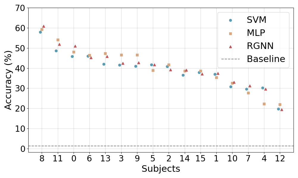
(a) The “all” task.

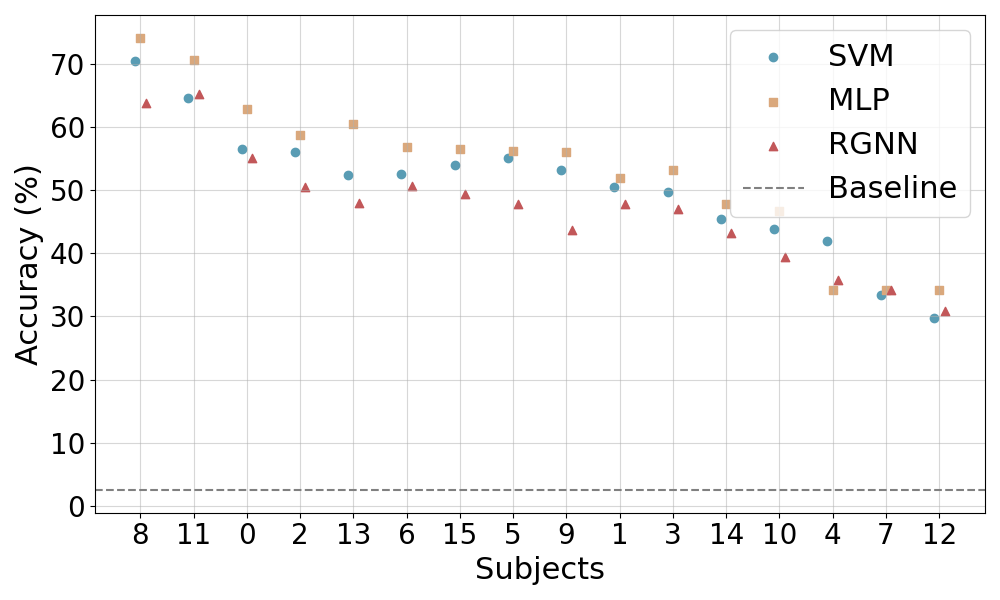
(b) The “coarse” task.

(c) The “fine” task.

Figure 4: Acc for each participant in the object classification task across SVM, MLP, and RGNN Models.

Figure 5 presents more image generation results selected from other participants, with Figure 5(a) showing good cases and Figure 5(b) showing bad cases. We identified three main types of bad cases. Similar to the first two images, the reconstructed images lack or misrepresent low-level information such as color and shape. These errors are relatively common and are due to the limitations of our feature mapper and the simple structure of the reconstruction pipeline, resulting in insufficient information restoration. Similar to the latter two images, the reconstructed images lack detail. This limitation is due to the number of denoising steps in the diffusion model and the inherently low signal-to-noise ratio of EEG signals.

We also observed that for certain categories, especially fine-grained ones, all test data points resulted in near-noise outputs, which drew our attention. When we directly input category labels as text prompts into Stable Diffusion 1.4, we found that the generated images had poor realism and three-dimensional structure. Figure 5(c) compares these images with those generated by our reconstruction pipeline from the training set. This improvement suggests that we can use EEG, which can be quickly and extensively obtained as human feedback signals, to enhance the performance of text-image pre-trained models or generative models. This will be the direction of future research.

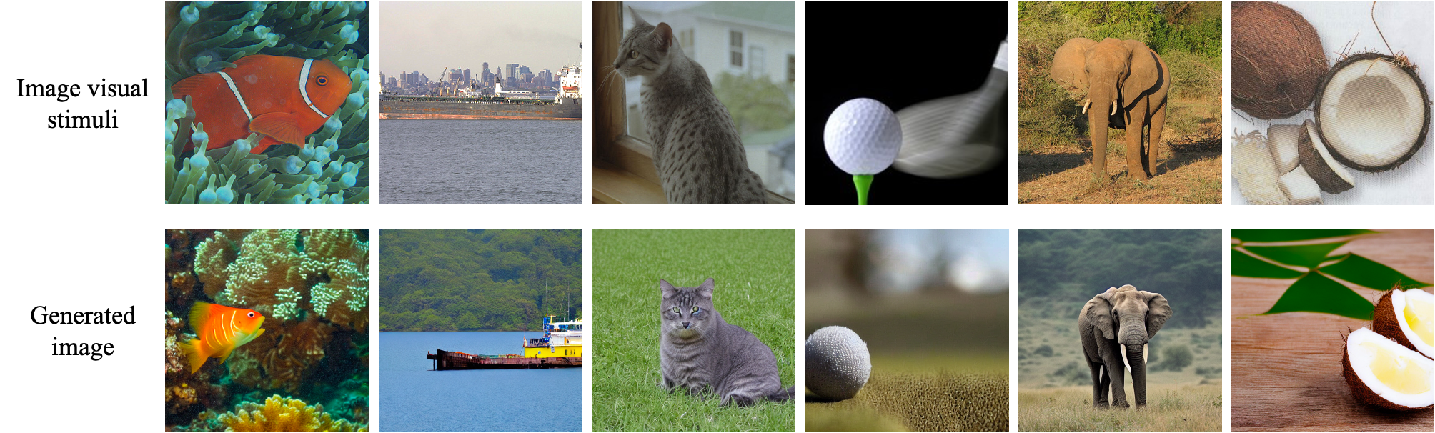
(a) Good cases.

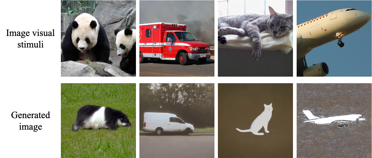
(b) Bad cases.

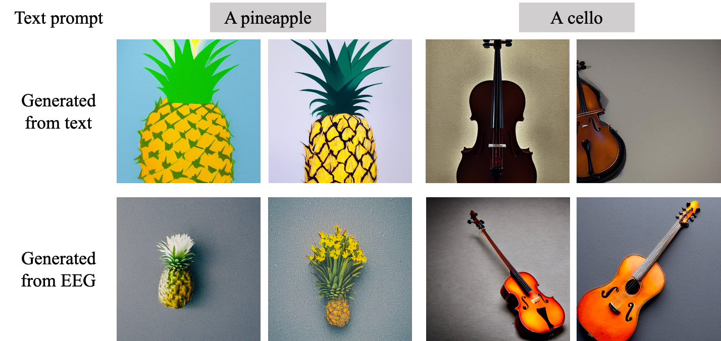
(c) Comparison of EEG and text-generated images.

Figure 5: More results in the image generation task.

A.5 Temporal Effect

In our experimental paradigm, to reduce the cognitive load on participants, we group images of the same category together and use the RSVP (Rapid Serial Visual Presentation) paradigm for continuous rapid stimulation. This approach may cause the model to learn temporal continuity features rather than the intrinsic characteristics of the category stimuli. In this study, we use narrower cropped time segments as input features and divide the training and test sets based on temporal order to reduce the impact of temporal effects. In Figure 6, we plotted the average classification accuracy for images at different index positions in the test set under various training and test set splits.

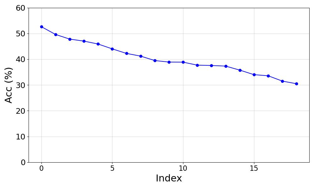
(a) 30/20 split for the training and test sets.

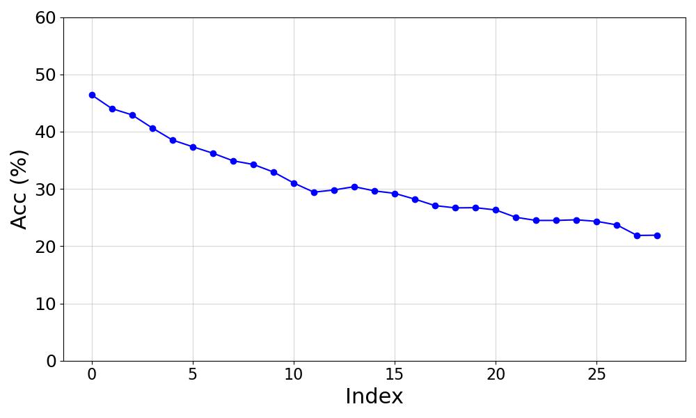
(b) 20/30 split for the training and test sets.

Figure 6: Average classification accuracy under different training and test set splits, with accuracy plotted against the indices of image stimuli in the test set.

We observed that the first few images in the test set have significantly higher accuracy, indicating a strong temporal effect, while the accuracy tends to stabilize for the subsequent images. Next, we also used several statistical methods for analysis. For the 30-20 split, we first calculated the sliding window standard deviation to measure local volatility. With a sliding window size of 5, the standard deviation at the 14th data point was less than 0.01, indicating a convergence trend at this point. We then checked the stationarity of the data using the ADF test, obtaining an ADF statistic of -1.1874 and a p-value of 0.6790, suggesting that the data might not have fully converged. For the 20-30 split, the standard deviation at the 16th data point was less than 0.01 with a sliding window size of 5. The ADF test yielded a statistic of -3.8505 and a p-value of 0.0024, indicating that the data is stationary and convergent.

In summary, EEG-ImageNet is subject to certain temporal effects. The methods we employed reduced this impact but did not completely eliminate it. Therefore, we recommend that all researchers using this dataset adopt preprocessing techniques similar to ours.

References

- Allen et al. [2022] Emily J Allen, Ghislain St-Yves, Yihan Wu, Jesse L Breedlove, Jacob S Prince, Logan T Dowdle, Matthias Nau, Brad Caron, Franco Pestilli, Ian Charest, et al. A massive 7t fmri dataset to bridge cognitive neuroscience and artificial intelligence. Nature neuroscience, 25(1):116–126, 2022.
- Antonello et al. [2024] Richard Antonello, Aditya Vaidya, and Alexander Huth. Scaling laws for language encoding models in fmri. Advances in Neural Information Processing Systems, 36, 2024.
- Benchetrit et al. [2023] Yohann Benchetrit, Hubert Banville, and Jean-Rémi King. Brain decoding: toward real-time reconstruction of visual perception. arXiv preprint arXiv:2310.19812, 2023.
- Chang et al. [2019] Nadine Chang, John A Pyles, Austin Marcus, Abhinav Gupta, Michael J Tarr, and Elissa M Aminoff. Bold5000, a public fmri dataset while viewing 5000 visual images. Scientific data, 6(1):49, 2019.
- Chen et al. [2015] Xinlei Chen, Hao Fang, Tsung-Yi Lin, Ramakrishna Vedantam, Saurabh Gupta, Piotr Dollár, and C Lawrence Zitnick. Microsoft coco captions: Data collection and evaluation server. arXiv preprint arXiv:1504.00325, 2015.
- Cheng et al. [2023] Fan L Cheng, Tomoyasu Horikawa, Kei Majima, Misato Tanaka, Mohamed Abdelhack, Shuntaro C Aoki, Jin Hirano, and Yukiyasu Kamitani. Reconstructing visual illusory experiences from human brain activity. Science Advances, 9(46):eadj3906, 2023.
- Duan et al. [2013] Ruo-Nan Duan, Jia-Yi Zhu, and Bao-Liang Lu. Differential entropy feature for eeg-based emotion classification. In 2013 6th international IEEE/EMBS conference on neural engineering (NER), pages 81–84. IEEE, 2013.
- Heeger and Ress [2002] David J Heeger and David Ress. What does fmri tell us about neuronal activity? Nature reviews neuroscience, 3(2):142–151, 2002.
- Horikawa and Kamitani [2017] Tomoyasu Horikawa and Yukiyasu Kamitani. Generic decoding of seen and imagined objects using hierarchical visual features. Nature communications, 8(1):15037, 2017.
- Jiang et al. [2015] Ming Jiang, Shengsheng Huang, Juanyong Duan, and Qi Zhao. Salicon: Saliency in context. In Proceedings of the IEEE conference on computer vision and pattern recognition, pages 1072–1080, 2015.
- Joshi and Guerzhoy [2017] Ujash Joshi and Michael Guerzhoy. Automatic photo orientation detection with convolutional neural networks. In 2017 14th Conference on Computer and Robot Vision (CRV), pages 103–108. IEEE, 2017.
- Kaneshiro et al. [2015] Blair Kaneshiro, Marcos Perreau Guimaraes, Hyung-Suk Kim, Anthony M Norcia, and Patrick Suppes. A representational similarity analysis of the dynamics of object processing using single-trial eeg classification. Plos one, 10(8):e0135697, 2015.
- Kannathal et al. [2005] N Kannathal, U Rajendra Acharya, Choo Min Lim, and PK Sadasivan. Characterization of eeg—a comparative study. Computer methods and Programs in Biomedicine, 80(1):17–23, 2005.
- Kay et al. [2008] Kendrick N Kay, Thomas Naselaris, Ryan J Prenger, and Jack L Gallant. Identifying natural images from human brain activity. Nature, 452(7185):352–355, 2008.
- Koelstra et al. [2011] Sander Koelstra, Christian Muhl, Mohammad Soleymani, Jong-Seok Lee, Ashkan Yazdani, Touradj Ebrahimi, Thierry Pun, Anton Nijholt, and Ioannis Patras. Deap: A database for emotion analysis; using physiological signals. IEEE transactions on affective computing, 3(1):18–31, 2011.
- Krizhevsky et al. [2009] Alex Krizhevsky, Geoffrey Hinton, et al. Learning multiple layers of features from tiny images. 2009.
- Lawhern et al. [2018] Vernon J Lawhern, Amelia J Solon, Nicholas R Waytowich, Stephen M Gordon, Chou P Hung, and Brent J Lance. Eegnet: a compact convolutional neural network for eeg-based brain–computer interfaces. Journal of neural engineering, 15(5):056013, 2018.
- Li et al. [2022] Junnan Li, Dongxu Li, Caiming Xiong, and Steven Hoi. Blip: Bootstrapping language-image pre-training for unified vision-language understanding and generation. In International conference on machine learning, pages 12888–12900. PMLR, 2022.
- Li et al. [2018] Ren Li, Jared S Johansen, Hamad Ahmed, Thomas V Ilyevsky, Ronnie B Wilbur, Hari M Bharadwaj, and Jeffrey Mark Siskind. Training on the test set? an analysis of spampinato et al.[31]. arXiv preprint arXiv:1812.07697, 2018.
- Lin et al. [2014] Tsung-Yi Lin, Michael Maire, Serge Belongie, James Hays, Pietro Perona, Deva Ramanan, Piotr Dollár, and C Lawrence Zitnick. Microsoft coco: Common objects in context. In Computer Vision–ECCV 2014: 13th European Conference, Zurich, Switzerland, September 6-12, 2014, Proceedings, Part V 13, pages 740–755. Springer, 2014.
- Liu et al. [2021] Yiqun Liu, Jiaxin Mao, Xiaohui Xie, Min Zhang, and Shaoping Ma. Challenges in designing a brain-machine search interface. In ACM SIGIR Forum, volume 54, pages 1–13. ACM New York, NY, USA, 2021.
- Logothetis [2008] Nikos K Logothetis. What we can do and what we cannot do with fmri. Nature, 453(7197):869–878, 2008.
- Logothetis et al. [2001] Nikos K Logothetis, Jon Pauls, Mark Augath, Torsten Trinath, and Axel Oeltermann. Neurophysiological investigation of the basis of the fmri signal. nature, 412(6843):150–157, 2001.
- Miranda-Correa et al. [2018] Juan Abdon Miranda-Correa, Mojtaba Khomami Abadi, Nicu Sebe, and Ioannis Patras. Amigos: A dataset for affect, personality and mood research on individuals and groups. IEEE transactions on affective computing, 12(2):479–493, 2018.
- Ozcelik and VanRullen [2023] Furkan Ozcelik and Rufin VanRullen. Natural scene reconstruction from fmri signals using generative latent diffusion. Scientific Reports, 13(1):15666, 2023.
- Radford et al. [2021] Alec Radford, Jong Wook Kim, Chris Hallacy, Aditya Ramesh, Gabriel Goh, Sandhini Agarwal, Girish Sastry, Amanda Askell, Pamela Mishkin, Jack Clark, et al. Learning transferable visual models from natural language supervision. In International conference on machine learning, pages 8748–8763. PMLR, 2021.
- Richards et al. [2019] Blake A Richards, Timothy P Lillicrap, Philippe Beaudoin, Yoshua Bengio, Rafal Bogacz, Amelia Christensen, Claudia Clopath, Rui Ponte Costa, Archy de Berker, Surya Ganguli, et al. A deep learning framework for neuroscience. Nature neuroscience, 22(11):1761–1770, 2019.
- Ridnik et al. [2021] Tal Ridnik, Emanuel Ben-Baruch, Asaf Noy, and Lihi Zelnik-Manor. Imagenet-21k pretraining for the masses. arXiv preprint arXiv:2104.10972, 2021.
- Rombach et al. [2022] Robin Rombach, Andreas Blattmann, Dominik Lorenz, Patrick Esser, and Björn Ommer. High-resolution image synthesis with latent diffusion models. In Proceedings of the IEEE/CVF conference on computer vision and pattern recognition, pages 10684–10695, 2022.
- Scotti et al. [2024] Paul Scotti, Atmadeep Banerjee, Jimmie Goode, Stepan Shabalin, Alex Nguyen, Aidan Dempster, Nathalie Verlinde, Elad Yundler, David Weisberg, Kenneth Norman, et al. Reconstructing the mind’s eye: fmri-to-image with contrastive learning and diffusion priors. Advances in Neural Information Processing Systems, 36, 2024.
- Shah et al. [2018] Vinit Shah, Eva Von Weltin, Silvia Lopez, James Riley McHugh, Lillian Veloso, Meysam Golmohammadi, Iyad Obeid, and Joseph Picone. The temple university hospital seizure detection corpus. Frontiers in neuroinformatics, 12:83, 2018.
- Spampinato et al. [2017] Concetto Spampinato, Simone Palazzo, Isaak Kavasidis, Daniela Giordano, Nasim Souly, and Mubarak Shah. Deep learning human mind for automated visual classification. In Proceedings of the IEEE conference on computer vision and pattern recognition, pages 6809–6817, 2017.
- St-Yves et al. [2023] Ghislain St-Yves, Emily J Allen, Yihan Wu, Kendrick Kay, and Thomas Naselaris. Brain-optimized deep neural network models of human visual areas learn non-hierarchical representations. Nature communications, 14(1):3329, 2023.
- Takagi and Nishimoto [2023] Yu Takagi and Shinji Nishimoto. High-resolution image reconstruction with latent diffusion models from human brain activity. In Proceedings of the IEEE/CVF Conference on Computer Vision and Pattern Recognition, pages 14453–14463, 2023.
- Tang et al. [2024] Jerry Tang, Meng Du, Vy Vo, Vasudev Lal, and Alexander Huth. Brain encoding models based on multimodal transformers can transfer across language and vision. Advances in Neural Information Processing Systems, 36, 2024.
- Teplan et al. [2002] Michal Teplan et al. Fundamentals of eeg measurement. Measurement science review, 2(2):1–11, 2002.
- Toneva et al. [2022] Mariya Toneva, Jennifer Williams, Anand Bollu, Christoph Dann, and Leila Wehbe. Same cause; different effects in the brain. arXiv preprint arXiv:2202.10376, 2022.
- Xiao et al. [2010] Jianxiong Xiao, James Hays, Krista A Ehinger, Aude Oliva, and Antonio Torralba. Sun database: Large-scale scene recognition from abbey to zoo. In 2010 IEEE computer society conference on computer vision and pattern recognition, pages 3485–3492. IEEE, 2010.
- Yao et al. [2019] Dezhong Yao, Yun Qin, Shiang Hu, Li Dong, Maria L Bringas Vega, and Pedro A Valdés Sosa. Which reference should we use for eeg and erp practice? Brain topography, 32:530–549, 2019.
- Ye et al. [2024] Ziyi Ye, Xiaohui Xie, Qingyao Ai, Yiqun Liu, Zhihong Wang, Weihang Su, and Min Zhang. Relevance feedback with brain signals. ACM Transactions on Information Systems, 42(4):1–37, 2024.
- Zhang et al. [2012] Haihong Zhang, Cuntai Guan, Kai Keng Ang, Chuanchu Wang, and Zheng Yang Chin. Bci competition iv–data set i: learning discriminative patterns for self-paced eeg-based motor imagery detection. Frontiers in neuroscience, 6:7, 2012.
- Zhang et al. [2024] Shaorun Zhang, Zhiyu He, Ziyi Ye, Peijie Sun, Qingyao Ai, Min Zhang, and Yiqun Liu. Eeg-svrec: An eeg dataset with user multidimensional affective engagement labels in short video recommendation. arXiv preprint arXiv:2404.01008, 2024.
- Zheng and Lu [2015] Wei-Long Zheng and Bao-Liang Lu. Investigating critical frequency bands and channels for eeg-based emotion recognition with deep neural networks. IEEE Transactions on autonomous mental development, 7(3):162–175, 2015.
- Zhong et al. [2020] Peixiang Zhong, Di Wang, and Chunyan Miao. Eeg-based emotion recognition using regularized graph neural networks. IEEE Transactions on Affective Computing, 13(3):1290–1301, 2020.