From many-body ab initio to effective excitonic models: a versatile mapping approach including environmental embedding effects

Abstract

We present an original multi-state projective diabatization scheme based on the Green’s function formalism that allows the systematic mapping of many-body ab initio calculations onto effective excitonic models. This method inherits the ability of the Bethe-Salpeter equation to describe Frenkel molecular excitons and intermolecular charge-transfer states equally well, as well as the possibility for an effective description of environmental effects in a QM/MM framework. The latter is found to be a crucial element in order to obtain accurate model parameters for condensed phases and to ensure their transferability to excitonic models for extended systems. The method is presented through a series of examples illustrating its quality, robustness, and internal consistency.

]Grenoble Alpes University, CNRS, Grenoble INP, Institut Néel, 25 rue des Martyrs, 38042 Grenoble, France ]Grenoble Alpes University, CNRS, Grenoble INP, Institut Néel, 25 rue des Martyrs, 38042 Grenoble, France ]Grenoble Alpes University, CNRS, Grenoble INP, Institut Néel, 25 rue des Martyrs, 38042 Grenoble, France DFT, BSE, CT, FE, e-h, TD-DFT, ET, HT, XET, XET

1 Introduction

The accurate first-principles description of elementary excitations (excitons) in organic materials represents an invaluable investigation tool for understanding their photophysical properties as well as phenomena underlying applications in optoelectronics, such as energy transfer, exciton splitting or charge separation in organic solar cells.^{1, 2, 3, 4}

Despite the outstanding progress over the last decades, the ab initio description of excitons in molecular systems still stands as a challenge for theory and computation, because of the difficulty in meeting accuracy and computational cost. A paradigmatic case is represented by the quest for relatively cheap methods able to describe equally well intra-molecular Frenkel-type excitons (FE) and inter-molecular charge transfer (CT) excitation, both characterizing the low-energy region of the excitation spectrum of molecular materials.

Time-dependent density-functional theory (TD-DFT), in its linear-response formulation within the adiabatic approximation,⁵ has been the most popular investigation method for the characterization of excitons in molecular systems. TD-DFT arguably represents one of the most reliable methods among those being computationally affordable for large and complex real-life materials. However, TD-DFT is known to present some limitations, such as the inaccurate and strongly functional-dependent description of CT excitations. This results in a possibly incorrect state ordering with FEs,^{6, 7} or in missing the characteristic Coulomb-like dependence of CT states energy with inter-molecular distance when using local, semilocal, or global hybrid functionals.⁸ These shortcomings can be significantly attenuated with the use of range-separated functionals,^{9, 10} leading to results that however depend on the the specific parameterization for the range separation of the Coulomb repulsion term.

Many-body perturbation methods based on Green’s function theory, such as the $GW$^{11, 12, 13, 14, 15, 16} and the Bethe-Salpeter equation (BSE) formalisms,^{17, 18, 19, 20} stand as robust and affordable options for computing the excited states in molecular systems.^{21, 22, 23, 24, 25, 26, 27, 28, 29, 30, 31} $GW$/BSE features the same $\mathcal{O}(N^{4})$ computational scaling with respect to the system size as TD-DFT and provides an accurate description for excitations of different nature thanks to a proper description of electronic correlations. Benchmark studies against reference methods and experimental data demonstrated a typical accuracy of 0.1-0.2 eV for charged and optical excitations.^{32, 33, 34, 35, 36, 37, 38, 39, 40, 41, 42, 43} Specifically, the explicit accounting for the non-local excitonic electron-hole interaction permits a faithful description of excitations regardless of their nature (FE vs. CT), of the type of system under scrutiny (e.g. organic homo- and hetero-molecular, inorganic, hybrid) and, importantly, of the functional used as starting point for the many-body perturbation theory.^{31, 36, 41}

The possibility of describing molecular excitations in condensed phases with Green’s function many-body method has been enabled by the recent development of a multiscale embedding method of different levels of detail, namely polarizable continuum model (PCM),^{44, 45, 46, 47} classical atomistic (polarizable QM/MM)^{48, 49, 30} and full-quantum (QM/QM’)^{50, 51}. Embedded $GW$ and BSE formalisms have been successfully applied in the contexts of molecular doping^{52, 53, 54, 55} and organic photovoltaics.⁵⁶ Many-body perturbation theory methods have been historically developed for extended (i.e. periodic) systems¹⁴ and applications to molecular solids have been reported in the literature.^{57, 58, 59, 60} These calculations are extremely expensive and hardly affordable for realistic molecular solids encompassing many atoms in the unit cell or featuring structural disorder.

Effective model Hamiltonians for excited states represent a cheap and insightful alternative to a full ab initio treatment for the description of the low-energy physics of multichromophoric systems.^{61, 3, 62, 63} These approaches rely on the definition of a reduced set of diabatic states characterized by wave functions localized on single molecular units, usually including pure intra-molecular FE and pure inter-molecular CT excitations with electron and hole localized on different fragments (see Figure 1). For this reason, these approaches are sometimes referred to as “low-energy” or “few-state” models. A typical model Hamiltonian for a molecular solid can be expressed as the sum of three terms,

$$\textrm{H}=\textrm{H}_{\mathrm{FE}}+\textrm{H}_{\mathrm{CT}}+\textrm{H}_{\mathrm{CT-FE}}\mathrm{,}$$ (1)

describing FEs (standard Frenkel exciton model), inter-molecular CT states, and the interaction between the two types of exciton (see SI for explicit expressions). Black arrows in Fig. 1 show the elementary processes corresponding to the quantum coupling between states, namely FE transfer(XT), excited-state hole/electron transfer (XHT/XET), and hole/electron transfer (HT/ET). The energy of the diabatic basis states and the coupling between them represent the parameters entering the FE-CT model Hamiltonian for excited states. Excitonic models, properly extended to include the coupling to quantum or classical vibrations find also application in the description of steady-state optical processes⁶² and real-time dynamics.^{64, 63, 65}

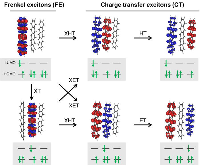
Figure 1: Basis diabatic states (pure FE and CT excitons) and main elementary processes defining effective exciton models for supramolecular systems, illustrated for a pentacene trimer extracted from the crystal structure. Hole/electron densities are shown in red/blue isosurfaces of the corresponding probability amplitude. Elementary processes include exciton transfer (XT) and one-body hole/electron transfer coupling FE and CT states (excited-state hole/electron transfer, XHT/XET) and CT states among themselves (hole/electron transfer, HT/ET). Gray boxes display the electronic configurations of basis states. For the sake of illustration, two-level (HOMO, LUMO) molecules have been considered.

The quality of first-principle calculations can be preserved to a large extent by computing the model parameters ab initio in the spirit of a multiscale approach.^{62, 63, 65} For instance, XT couplings between singlet excitons are the only parameters in play in the standard FE model, and several methods have been proposed to its calculations at various levels of theory.⁶⁶ The simplest approach is the so-called dimer splitting method that, however, strictly applies only to pairs of molecules equivalent by symmetry, each of which presents excitons well-separated in energy. A common approximation consists of neglecting the contributions due to the inter-molecular overlap (exchange terms, e.g. Dexter) and retaining the Coulomb, Förster-type, interaction between the transition densities of FEs, which is the leading term at a large inter-molecular distance. Point-dipole and distributed-monopole⁶⁷ approximations of the transition density offer practical schemes for computing this interaction.

Whenever inter-molecular overlap is of concern, or for more complex FE-CT exciton models, the derivation of parameters from first-principles usually follows so-called diabatization schemes,^{68, 69, 70, 71, 64, 72, 73, 74, 75, 76, 77} in which a unitary transformation is defined transforming the diagonal adiabatic representation of the Hamiltonian of the multichromophoric system into the diabatic one, featuring diabatic-states energies on the diagonal and the couplings among them elsewhere. The choice of the unitary transformation is somewhat arbitrary. Common choices employ the eigenstates of a physically-motivated observable (e.g. in the popular fragment excitation difference scheme, FED⁷⁰), or projective schemes where suitable basis functions are introduced.^{72, 64, 77} Projective schemes based on BSE/$GW$ calculations, within the Tamm-Dancoff approximation (TDA),^{78, 79} have been proposed by Wehner and Baumeier⁸⁰ and Leng et al..⁸¹ schemes in a very recent work.⁸² Full and TDA BSE/$GW$ calculations have been very recently combined with common diabatization methods (Edmiston-Ruedenberg,⁸³ generalized Mulliken-Hush,⁶⁸ fragment charge difference⁸⁴) by Tirimbó and Baumeier.⁸²

In this work, we present an original projection-based diabatization scheme based on the BSE/$GW$ formalism, beyond the TDA. The method is designed to be generally applicable to systems with an arbitrary number of excited states of both FE and CT nature. A distinctive feature of our methodology is the employ of QM/MM embedding techniques for building effective excitonic models for systems in condensed phases. Special emphasis is put on the transferability of the parameters obtained for small molecular clusters (dimers or trimers) to excitonic models for extended systems. The use of classical MM embedding turns out to be essential for such a purpose. Overall, the proposed methodology provides a general, robust, and versatile framework for the systematic mapping of many-body ab initio calculations to effective excitonic models for large supramolecular systems such as solids, films, and interfaces.

2 Theory

2.1 $GW$ and Bethe–Salpeter equation formalism

The present development aims to set up effective excitonic models within the framework of the many-body ab initio Green’s function techniques $GW$ and BSE. This subject is briefly outlined here from a practical perspective, highlighting the features that will be mostly relevant to this end. For further detail, we refer the readers to review papers^{14, 31, 15, 16} and to the original publications of our implementation.^{23, 24, 44, 48, 49}

Methods based on Green’s functions rely on many-body perturbation theory to compute electronic excitations upon introducing electronic correlation effects on top of mean-field electronic structure calculations, such as Kohn-Sham DFT. ⁸⁵ The set of Kohn-Sham orbitals $\{\phi^{\mathrm{KS}}\}$ and one-particle energies $\{\varepsilon^{\mathrm{KS}}\}$ obtained with a given functional approximation define the non-interacting system used as a starting point for the perturbation theory. Then, within this framework, charged excitations such as electron removal (e.g. ionization potential) and electron addition (e.g. electron affinity) can be computed as quasiparticle energies

$$\varepsilon_{n}=\varepsilon^{\mathrm{KS}}_{n}+\langle\phi_{n}|\Sigma(\varepsilon_{n})-V_{xc}|\phi_{n}\rangle,$$ (2)

where, in practice, the self energy $\Sigma(\varepsilon_{n})$ replaces the Kohn-Sham DFT exchange-correlation potential $V_{xc}$. The self-energy is a non-local and energy-dependent operator, $\Sigma({\bf r},{\bf r}^{\prime};\varepsilon)$. This, within the $GW$ formalism, is approximated as the product of the single-particle Green’s function ($G$) and the screened Coulomb interaction ($W$), i.e. $\Sigma^{GW}=\textrm{i}GW$ with i being the imaginary unit. In the so-called $G_{0}W_{0}$ scheme, $\Sigma^{GW}$ is built directly with the Kohn-Sham levels. Re-computing the self-energy with quasiparticle energies iteratively until convergence leads to the partially self-consistent ev$GW$ scheme. This approach largely reduces the dependence of quasiparticle excitations on the starting DFT functional, leading to a good agreement with experimental values or high-level CCSD(T) calculations.^{32, 40, 86}

Neutral excitations can be obtained via the BSE, which is a two-body correlated electron-hole (e-h) problem described by the following non-Hermitian eigenvalue equation

$$\left(\begin{array}[]{cc}\mathbf{A}&\mathbf{B}\\ \mathbf{B}^{*}&\mathbf{A}^{*}\end{array}\right)\left(\begin{array}[]{c}\mathbf{X}_{k}\\ \mathbf{Y}_{k}\end{array}\right)=\Omega_{k}\left(\begin{array}[]{c}\mathbf{X}_{k}\\ \mathbf{Y}_{k}\end{array}\right)$$ (3)

where $\Omega_{k}$ is the excitation energy of the $k$-th state, the corresponding eigenvector including an excitation ($\mathbf{X}_{k}$, occupied $\rightarrow$ virtual) and a de-excitation ($\mathbf{Y}_{k}$, virtual $\rightarrow$ occupied) component. For singlet excitations, the resonant and anti-resonant blocks of the BSE Hamiltonian reads:

$$A_{ai,bj} = \delta_{ab}\delta_{ij}\left(\varepsilon_{a}^{GW}-\varepsilon_{i}^{GW}\right)+2\left\langle\phi_{a}(\mathbf{r})\phi_{j}\left(\mathbf{r}^{\prime}\right)|v\left(\mathbf{r},\mathbf{r}^{\prime}\right)|\phi_{i}(\mathbf{r})\phi_{b}\left(\mathbf{r}^{\prime}\right)\right\rangle$$ (4)

$$- \left\langle\phi_{a}(\mathbf{r})\phi_{j}\left(\mathbf{r}^{\prime}\right)|W\left(\mathbf{r},\mathbf{r}^{\prime},\omega=0\right)|\phi_{b}(\mathbf{r})\phi_{i}\left(\mathbf{r}^{\prime}\right)\right\rangle$$

$$B_{ai,bj} = 2\left\langle\phi_{a}(\mathbf{r})\phi_{b}\left(\mathbf{r}^{\prime}\right)|v\left(\mathbf{r},\mathbf{r}^{\prime}\right)|\phi_{i}(\mathbf{r})\phi_{j}\left(\mathbf{r}^{\prime}\right)\right\rangle$$ (5)

$$- \left\langle\phi_{a}(\mathbf{r})\phi_{b}(\mathbf{r}^{\prime})|W\left(\mathbf{r},\mathbf{r}^{\prime},\omega=0\right)|\phi_{j}\left(\mathbf{r}\right)\phi_{i}\left(\mathbf{r}^{\prime}\right)\right\rangle$$

where $v({\bf r},{\bf r}^{\prime})=1/|\mathbf{r}-{\mathbf{r}}^{\prime}|$ is the bare Coulomb interaction and $W$ is the screened one in the static limit ($\omega=0$). Let us comment that the Kohn-Sham orbitals $\{\phi_{n}\}$ are real-valued in the present work. The anti-resonant blocks $\mathbf{B}$ and $\mathbf{B}^{*}$ are neglected in the Tamm-Dancoff approximation ^{78, 79}, which is not adopted in this work. We emphasize that the screened-Coulomb potential matrix elements in the resonant block $\mathbf{A}$ do not cancel when occupied $(i,j)$ states do not overlap with unoccupied $(a,b)$ states. This explains the success of BSE for CT excitations.

BSE eigenvectors are normalized (i.e. $\sum_{ia}\left[(X_{k}^{ia})^{2}-(Y_{k}^{ia})^{2}\right]=1$) and orthogonal to each other, allowing us to define the two-body (electron-hole) exciton wavefunction as

$$\Psi_{k}(\mathbf{r}_{\mathrm{h}},\mathbf{r}_{\mathrm{e}})=\sum_{ia}\left\{X_{k}^{ia}\phi_{i}(\mathbf{r}_{\mathrm{h}})\phi_{a}(\mathbf{r}_{\mathrm{e}})+Y_{k}^{ia}\phi_{i}\ (\mathbf{r}_{\mathrm{e}})\phi_{a}(\mathbf{r}_{\mathrm{h}})\right\}$$ (6)

and the corresponding transition density

$$n_{k}^{\textrm{T}}({\bf r})=\sqrt{2}\sum_{ia}(X_{k}^{ia}+Y_{k}^{ia})\phi_{i}({\bf r})\phi_{a}({\bf r}).$$ (7)

We recall that, despite the similarity between equation 3 and the popular Casida’s linear-response equation in TD-DFT,⁵ the explicit account for e-h interaction permits a faithful description of excitations, regardless of their nature (FE or CT) or of the Kohn-Sham-DFT functional approximation employed to construct the single-particle basis. This determines an important qualitative and quantitative improvement over TD-DFT, especially for the stability of CT excitation energies, making BSE a robust and predictive tool for describing FE and CT excitons on an equal footing.⁸⁷

2.2 Environmental embedding in $GW$/BSE

Many-body calculations of molecules and small molecular clusters in condensed phases have been performed by adopting hybrid quantum mechanics/classical mechanics (QM/MM) embedding techniques.^{44, 48, 49, 31} These approaches require accounting for the effect of the embedding environment at different steps of the computational workflow, first at the ground-state Kohn-Sham DFT level and then in the calculation of charged and neutral excitations.

Environmental embedding in the ground state is essential for molecules dissolved in polar solvents, as well as in the solid state. Ground-state electrostatic embedding is indeed necessary to describe the strong crystal fields sourced by molecular multipole moments. A proper description of internal fields is essential for the quantitative description of the absolute binding energies in photoemission experiments on molecular solids,⁴⁹ as well as to capture the dependence of energy levels on molecular orientations at film and crystal surfaces.⁵⁶ In the following, ground-state embedding will be either based on PCM,⁴⁴ to describe a generic non-polar medium, or on the charge response polarizable atomistic model,^{88, 89} whenever molecular crystals are the explicit target.

The treatment of the screening of charged ($GW$) and neutral (BSE) excitations in the presence of an environment has been documented in our original works.^{44, 48, 49} The key for this development consists in treating the dielectric susceptibility of the embedding medium as a frequency-independent quantity, i.e. the environment reacting instantaneously to the excitations within the QM region. The frequency-independent response of the environment is fully consistent with the BSE, which also relies on a static screening of the e-h interaction (see Eq. 4). The susceptibility is instead an explicitly dynamic quantity in the $GW$ formalism, requiring an additional step for combining the dielectric response of QM and MM regions. The effect of the screening of charged excitations (polarization energy) can be computed at the static COHSEX level, i.e. the frequency-independent analog of $GW$.¹¹

In previous works, the state-specific polarization energy was computed as the difference between the quasiparticle energy obtained in two independent COHSEX calculations including or not the effect of the environment. Then, this difference was added as a perturbative correction to $GW$ quasiparticle energies ($\Delta$COHSEX).^{48, 49} An alternative treatment of the environment emerged in the context of a QM/QM’ framework based on a fragment formalism.⁵¹ This approach allows an explicit account for the dynamics of the embedding medium (frequency $\omega_{\mathrm{env}}$), but also to recover the instantaneous dielectric response of the environment in the $\omega_{\mathrm{env}}\rightarrow\infty$ limit. This permits the description of the dielectric embedding beyond the perturbative $\Delta$COHSEX approach. The novel self-consistent COHSEX treatment of environmental screening has been combined with PCM and adopted in the present work. The details of the methodology will be disclosed in a forthcoming publication.

A central quantity in embedded $GW$/BSE is the so-called reaction field matrix, $v_{\mathrm{reac}}(\mathbf{r},\mathbf{r}^{\prime})$, describing the electric potential generated by the environment at a probe point $\mathbf{r}$ in response to a source charge at $\mathbf{r}^{\prime}$. The reaction field matrix can be written as

$$v_{\mathrm{reac}}(\mathbf{r},\mathbf{r}^{\prime})=\int d\mathbf{r}_{2}d\mathbf{r}_{2}^{\prime}\;v(\mathbf{r},\mathbf{r}_{2})\chi_{\mathrm{MM}}(\mathbf{r}_{2},\mathbf{r}_{2}^{\prime})v(\mathbf{r}_{2}^{\prime},\mathbf{r}^{\prime}),$$ (8)

where $\chi_{\mathrm{MM}}(\mathbf{r}_{2},\mathbf{r}_{2}^{\prime})$ is the interacting susceptibility of the environment alone. For PCM embedding, Eq. 8 corresponds to the interaction of a probe charge with the charge density induced by the source charge on the surface of the cavity. In embedded $GW$ and BSE calculations, the MM environment renormalizes the Coulomb potential within the QM region, i.e. $v\leftarrow v+v_{\mathrm{reac}}$.

In summary, in the following, we will perform embedded DFT/$GW$/BSE calculations using different schemes. PCM embedding has been used at every level of the calculation for model dimers reported in Section 3.1. A hybrid scheme has been instead adopted for structures extracted from crystal structures, see Section 3.2. In this case, an atomistic embedding has been adopted in the DFT calculation, to ensure a proper description of crystal fields in the neutral ground state, while the screening of excitations has been treated at the PCM level. The latter should be considered as an approximation of the anisotropic dielectric response of the crystal that is adopted for practical reasons.

2.3 Projective diabatization method

Given a reduced set of physically-motivated excitonic basis functions including FE and CT states, our aim is to obtain the matrix representation of an effective model Hamiltonian such that it reproduces excitation energies and wavefunctions of a BSE calculation on a small supramolecular cluster. Diabatic basis functions with excitons and charges localized on single molecular units (fragments) can be normalized but are not orthogonal to each other, requiring accounting for their overlap in a generalized eigenvalue problem. Keeping into explicit account the overlap among basis functions is actually an important ingredient for our long-term goal, which is to build models for large supramolecular clusters or extended systems in a modular fashion, namely using matrix elements derived only from BSE calculations on dimers or small aggregates. This procedure further allows one to systematically expand the system by simply adding additional basis functions to our set and deriving the corresponding effective Hamiltonian and overlap matrix elements without having to reconsider the coefficients already at hand.

We consider a system composed of distinct molecular fragments, where we perform BSE calculations on the single fragments and for the whole system. For the sake of simplicity, a system composed of two fragments (dimer) is considered in the following. The generalization to ensembles of more fragments is straightforward. We define a set of e-h states $\{\psi\}$ that will be used as a diabatic basis to set up the exciton-model Hamiltonian, including FE excitons localized on one of the two fragments and inter-fragment CT states. Diabatic FE states are set to the BSE eigenstates of individual fragments, with $\psi_{l}^{\mu}=\Psi_{l}^{\mu}(\mathbf{r}_{\mathrm{h}},\mathbf{r}_{\mathrm{e}})$ corresponding to the $l$th exciton of fragment $\mu$. CT basis states are defined as $\psi_{ia}^{\mu,\nu}(\mathbf{r}_{\mathrm{h}},\mathbf{r}_{\mathrm{e}})={\phi_{i}^{\mu}}(\mathbf{r}_{\mathrm{h}}){\phi_{a}^{\nu}}(\mathbf{r}_{\mathrm{e}})$ with $i$ referring to an occupied Kohn-Sham orbital of fragment $\mu$ and $a$ to a virtual state of fragment $\nu$. The number of selected FE and CT basis states (problem dimension $D$, fixed by the range spanned by $l$, $a$ and $i$) can be determined a posteriori, based on the energy range the model is expected to cover.

To build the low-energy Hamiltonian, we first introduce the overlap matrix between basis functions $\psi_{p}$ (hereafter identified with a single index $p=1,2\dots D$)

$$S_{pq}=\langle\psi_{p}|\psi_{q}\rangle,$$ (9)

and the projection matrix

$$P_{kq}=\langle\Psi_{k}|\psi_{q}\rangle$$ (10)

where $\Psi_{k}$ are the BSE eigenstates of the dimer with associated eigenvalues $\Omega_{k}$. The target eigenstates for the model Hamiltonian $\widetilde{\Psi}_{k}$, corresponding to the projection of BSE wavefunctions in the vector space spanned by the basis, are expressed as a linear combination of the diabatic states,

$$\widetilde{\Psi}_{k}=\sum_{p}C_{pk}\ \psi_{p},$$ (11)

the matrix of the expansion coefficients being

$$\mathbf{C}={\bf S}^{-1}\mathbf{P}\boldsymbol{\Lambda}.$$ (12)

This expression directly follows from the application to $\widetilde{\Psi}_{k}$ of the identity operator, in the form of a completeness relation for a non-orthogonal basis. The diagonal matrix $\boldsymbol{\Lambda}$, with elements $\Lambda_{kj}=|\widetilde{\Psi}_{k}|^{-1}\delta_{kj}$, ensures the normalization of the target functions, but not their orthogonality. We insist on the fact that while the BSE wavefunctions of the dimer ($\Psi_{k}$) form an orthonormal set, the target eigenstates for the model Hamiltonian ($\widetilde{\Psi}_{k}$) do not. Starting from such a common background, two methods can be proposed to obtain the Hamiltonian.

A straightforward approach consists of obtaining the Hamiltonian directly from the generalized eigenvalue equation as

$$\mathbf{H}=\mathbf{SC}\boldsymbol{\Omega}\mathbf{C}^{-1}$$ (13)

where $\boldsymbol{\Omega}$ is the diagonal matrix of the BSE eigenvalues. However, because of the non-orthogonality of $\tilde{\Psi}_{k}$ functions, the resulting $\mathbf{H}$ matrix is not symmetric as it should be. When asymmetry is small, as expected from a reasonably large basis set, a practical workaround could be the symmetrization by hand, i.e. $\mathbf{H}\leftarrow(\mathbf{H}+\mathbf{H}^{\mathrm{T}})/2$, where ${\bf H}^{\textrm{T}}$ is the transpose of ${\bf H}$.

Alternatively, we may recognize that the transpose of the Hamiltonian should also lead to the same eigenvalue problem (i.e. ${\bf H}^{\textrm{T}}{\bf C}={\bf SC}{\boldsymbol{\Omega}}$). Therefore, we can formulate this as the optimization problem of finding a symmetric Hamiltonian ${\bf H}$ as

$$\min_{{\bf H}}\left[||{\bf HC}-{\bf SC}{\boldsymbol{\Omega}}||+||{\bf H}^{\textrm{T}}{\bf C}-{\bf SC}{\boldsymbol{\Omega}}||\right],$$ (14)

where $||{\bf Z}||=\textrm{Tr}({\bf Z}^{\textrm{T}}{\bf Z})$ and Tr denotes the trace of the matrix ${\bf Z}$. Then, expressing Eq. 14 in terms of traces of product of matrices and following the usual rules for the derivatives of matrices ⁹⁰, we arrive at

$${\bf CC}^{\textrm{T}}{\bf H}+{\bf H}{\bf CC}^{\textrm{T}}={\bf C}{\boldsymbol{\Omega}}{\bf C}^{\textrm{T}}{\bf S}+{\bf SC}{\boldsymbol{\Omega}}{\bf C}^{\textrm{T}}$$ (15)

that corresponds to a Sylvester’s equation ⁹¹, which allows us to find the Hamiltonian ${\bf H}$ that is symmetric and best reproduces BSE eigenvalues and the target functions. Equation 15 can be solved with the Bartels–Stewart algorithm,⁹² see SI for details.

2.4 Approximate FE-FE and FE-CT exciton couplings

Besides the projective diabatization scheme described above, we also compute exciton couplings within common approximations. In the limit of zero intermolecular overlap, the coupling between singlet FE excitons reduces to the electrostatic interaction between transition densities.⁶¹ For a pair of molecules in the vacuum the FE-FE coupling is

$$V^{n-n}_{\mathrm{FE-FE}}(n_{\mu}^{\textrm{T}},n_{\nu}^{\textrm{T}})=\int d{\bf r}d{\bf r}^{\prime}n_{\mu}^{\textrm{T}}({\bf r})v({\bf r},{\bf r}^{\prime})n_{\nu}^{\textrm{T}}({\bf r}^{\prime})$$ (16)

where $n_{\mu}^{\textrm{T}}$ is the transition density of a given excitation on fragment $\mu$. Following a multipole expansion of $n_{\mu}^{\textrm{T}}$ truncated to the leading term, one obtains the coupling as the interaction between transition dipoles (${\bf d}_{\mu}^{\textrm{T}}$) as

$$V^{\mathrm{d-d}}_{\mathrm{FE-FE}}=\frac{|{\bf d}_{\mu}^{\textrm{T}}|\;|{\bf d}_{\nu}^{\textrm{T}}|}{|{\bf R}_{\mu\nu}|^{3}}\left[\widehat{{\bf d}}_{\mu}^{\textrm{T}}\cdot\widehat{{\bf d}}_{\nu}^{\textrm{T}}-3(\widehat{{\bf d}}_{\mu}^{\textrm{T}}\cdot\widehat{\bf R}_{\mu\nu})(\widehat{{\bf d}}_{\nu}^{\textrm{T}}\cdot\widehat{\bf R}_{\mu\nu})\right],$$ (17)

where ${\bf R}_{\mu\nu}$ is the inter-fragment distance and hat symbol denotes unit vectors. The dipolar approximation holds at a large distance, with a characteristic $|{\bf R}_{\mu\nu}|^{-3}$ decay of the coupling.

The presence of an embedding environment (e.g. PCM) affects the electrostatic coupling in two ways, as discussed by Mennucci and coworkers. ^{93, 94} The first trivial effect, results from the change in the transition density of each molecular fragment due to the embedding polarizable medium. The second contribution results from the dielectric screening of the field exerted by the transition densities. Both effects are considered in our calculations, namely, transition densities are obtained from embedded BSE calculations and screened couplings are computed as

$${V}^{n-n,\mathrm{e}}_{\mathrm{FE-FE}}(n_{\mu}^{\mathrm{T,e}},n_{\nu}^{\mathrm{T,e}})=\int d{\bf r}d{\bf r}^{\prime}\ n_{\mu}^{\mathrm{T,e}}({\bf r})\left[v({\bf r},{\bf r}^{\prime})+v_{reac}({\bf r},{\bf r}^{\prime})\right]n_{\nu}^{\mathrm{T,e}}({\bf r}^{\prime}),$$ (18)

where the superscript ”e” labels quantities calculated in the environment and $v_{reac}({\bf r},{\bf r}^{\prime})$ is the medium reaction field defined in Equation 8 that here is calculated at the PCM level. Following Mennucci and coworkers,^{94, 93} we introduce an effective screening factor

$$s=\frac{V^{n-n,\mathrm{e}}_{\mathrm{FE-FE}}(n_{\mu}^{\mathrm{T,e}},n_{\nu}^{\mathrm{T,e}})}{V^{n-n}_{\mathrm{FE-FE}}(n_{\mu}^{\mathrm{T,e}},n_{\nu}^{\mathrm{T,e}})}$$ (19)

where the screened and unscreened interactions are both computed for the same transition densities.

The screening factor $s$ can be evaluated for any transition density and polarizable embedding model. It is interesting to consider the case of point transition dipoles in a continuum dielectric. For dipoles incorporated in the dielectric, without an explicit cavity, the screening factor is $s=1/\epsilon_{\mathrm{opt}}$. In the limit of the large distance between the two dipoles enclosed into spherical cavities, the screening factor reads

$$s=\epsilon_{\mathrm{opt}}\left(\frac{3}{1+2\epsilon_{\mathrm{opt}}}\right)^{2}$$ (20)

where $\epsilon_{\mathrm{opt}}$ is the relative permittivity in the optical range. This expression is derived in the Appendix. To the best of our knowledge, this result has not been reported before. We have explicitly verified the agreement between Equation 20 and numerical calculations based on our PCM implementation.⁴⁴ For dipoles located at the cavity center, the limiting values are quickly recovered for dipole-dipole distances larger than twice the cavity radius, i.e. once the two dipoles are embedded in separate cavities. We emphasize that two elements concur to the result in Equation 20: (i) the screening of the field of one of the dipoles (source dipole) by the charges induced on the surface of its cavity; (ii) the Onsager cavity field generated within the cavity hosting the probe dipole by the (screened) field of the source dipole.⁹⁵

The FE-CT and some of the CT-CT couplings can be approximated as the matrix elements of the Kohn-Sham Hamiltonian between frontier molecular orbitals of the involved fragments. Referring to the example in Figure 1 for two-level molecules (HOMO, LUMO), the one-electron approximation for the coupling associated with XHT and HT process between fragments $\mu$ and $\nu$ is $\langle\phi_{\mathrm{HOMO}}^{\mu}|\widehat{\textrm{H}}_{\textrm{KS}}^{\mu\nu}|\phi_{\mathrm{HOMO}}^{\nu}\rangle$, where $\widehat{\textrm{H}}_{\textrm{KS}}^{\mu\nu}$ is the Kohn-Sham Hamiltonian for the dimer $\mu$-$\nu$ and $\phi_{\mathrm{HOMO}}^{\mu}$ is HOMO of fragment $\mu$. Similarly, the matrix element for XET and ET processes reads $\langle\phi_{\mathrm{LUMO}}^{\mu}|\widehat{\textrm{H}}_{\textrm{KS}}^{(\mu\nu)}|\phi_{\mathrm{LUMO}}^{\nu}\rangle$.

2.5 Computational details

In this work, we performed PBE0 calculations ^{96, 97} using the ORCA package ⁹⁸ to obtain the Kohn-Sham wavefunctions. $GW$ and BSE calculations were carried out with the BeDEFT program.⁹⁹ All calculations were done with the def2-TZVP basis set ¹⁰⁰ a the corresponding def2-TZVP-RI auxiliary basis for Coulomb fitting in the resolution-of-the-identity framework (RI-V)¹⁰¹. ev$GW$ calculations have been performed, correcting 4, 8, and 12 states in calculations of single fragments, dimers, and trimers, respectively. For PCM embedding, we adopted a dielectric constant $\epsilon_{r}=\epsilon_{\mathrm{opt}}=3.5$, typical of non-polar organic solids. Other parameters were set to the default values for benzene from the Minnesota Solvent Descriptor Database. DFT calculations employed the ORCA-code implementation of the conductor-like polarizable continuum model (C-PCM).¹⁰² A double-layer formulation of the integral equation formalism PCM model (IEF-PCM), allowing for charge-spilling effects, has been used in $GW$ and BSE computations.⁴⁴ The ground-state embedding of calculations on the pentacene crystal employed the charge response model⁸⁸ as implemented in the MESCal code.⁸⁹ The pentacene molecular geometry employed in model dimer calculations (Section 3.1) has been optimized at the B3LYP/def2-TZVP level in the gas phase. Dimers have been then built by creating a translated replica of the molecule along the direction perpendicular to the molecular plane, obtaining parallel co-facial dimers for different intermolecular distances. Calculations on the pentacene crystal (Section 3.2) have been performed for the Siegriest triclinic structure¹⁰³.

3 Results

We now present some illustrative examples of the application of our methodology for deriving effective excitonic models from many-body BSE/$GW$ calculations. Pentacene is taken as an ideal test case given its prominent role in organic electronic research. The following test cases allow us to discuss the merits of our approach, from the perspective of applying our methodology to supramolecular systems in the condensed phase. Selected examples include molecular homodimers in the vacuum and PCM, as well as the pentacene molecular crystal.

Effective model Hamiltonians are obtained with the diabatization method based on the optimization approach (solution of Equation 15). We emphasize that the diagonalization of the model Hamiltonian allows reproducing with high precision the target eigenvalues ($\Omega_{k}$) and eigenvectors ($\widetilde{\Psi}_{k}$) from BSE calculations. We have also considered the Hamiltonian obtained via Equation 13 and subsequent symmetrization by hand. The differences in the eigenvalues of the model $\mathbf{H}$ obtained with the two methods aretypically below 1 meV, which is practically negligible if compared to the approximation inherent to a few-state model or the intrinsic precision of BSE/$GW$ calculations. The optimization method is preferred, being a more rigorous and elegant approach.

3.1 Model molecular dimers

3.1.1 Pentacene homodimer in vacuum

We first analyze the case of a molecular homodimer in the vacuum. We consider molecular pairs arranged in a parallel cofacial geometry, with the intermolecular stacking distance $R$ scanned from 3.5 to 15 Å. The primary excitations of pentacene homodimers can be described in terms of two FE excitations, i.e. the $S_{1}$ excitons of the isolated fragments, and two CT states, corresponding to HOMO$\to$LUMO intermolecular transitions. Our basis to set up the model $\mathbf{H}$ is set accordingly, resulting in a 4-state model.

A distinctive aspect of our methodology is that a single (DFT, ev$GW$, BSE) calculation is performed for one of the two symmetry-equivalent molecules in the dimer, the second being created as a copy of the first one. This means that the atomic orbitals, Kohn-Sham orbitals, and BSE wavefunctions of fragment 2 are a translated replica of those of fragment 1. This fixes a convention for the phase of the basis excitonic functions that define the sign of the off-diagonal terms of $\mathbf{H}$ (excitonic couplings). This will be particularly important for calculations on crystals, as discussed later in Section 3.2.

Having defined the basis, BSE calculations can be performed on the dimer to obtain the excitonic model Hamiltonian according to the procedure described in Section 2.3. For example, the upper-triangular part of the Hamiltonian (in eV) at $R=5$ Å  one obtains

$${\bf H}_{\mathrm{pen-pen}}=\ \ \NiceArray{rrrrl}\mathrm{FE}_{1}&\mathrm{FE}_{2}\mathrm{CT}_{1\to 2}\mathrm{CT}_{2\to 1}\\ 1.8980.022-0.0260.057\mathrm{FE}_{1}\\ 1.8980.057-0.026\mathrm{FE}_{2}\\ 2.9230.000\mathrm{CT}_{1\to 2}\\ 2.923\mathrm{CT}_{2\to 1}\\ \CodeAfter\SubMatrix({2-1}{5-4})$$ (21)

which upon diagonalization yields eigenvalues that reproduce the 4 lowest-energy singlet BSE excitation energies (i.e. 1.870, 1.920, 2.924, and 2.930 eV) within 1 meV tolerance. The diagonal elements in Eq. LABEL:e:Heff2 represent the diabatic energies that are plotted for different inter-fragment distances in Fig. 2a, together with the BSE energies and the ev$GW$ HOMO-LUMO gap. We observe that the diabatic energies follow the behavior expected from fundamental physical considerations. The diabatic energies of the two localized FEs remain constant with the inter-fragment distances, rapidly approaching the two degenerate FEs of the dimer in the $R\to\infty$ limit. The diabatic energy of CT states follows the $1/R$ behavior prescribed by the e-h interaction for these intermolecular excitons, converging toward the photoemission gap at large $R$. The diabatic energies converge to the adiabatic dimer excitation energies for $R\to\infty$, while excitonic couplings determine significant deviations at distances typical of intermolecular contacts.

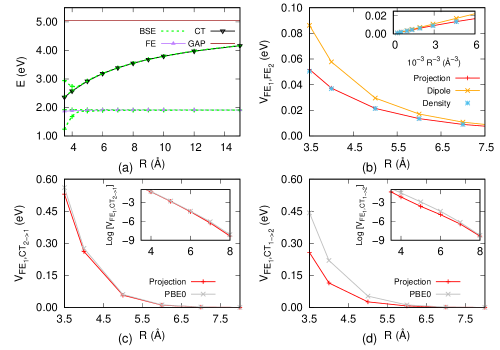
Figure 2: Results of the projective diabatization method for a pentacene dimer in the gas phase as a function of the inter-fragment distance $R$. (a) Diabatic energies compared to the BSE transition energies and to the ev$GW$ HOMO-LUMO gap. (b) FE-FE couplings as obtained with the diabatization scheme and as Coulomb interaction between transition densities and transition dipoles. (c-d) FE-CT couplings (absolute values) including the approximate one-electron matrix elements obtained at the PBE0 level.

The off-diagonal elements of the Hamiltonian correspond to FE-FE, FE-CT, and CT-CT couplings. The FE-FE couplings obtained at different inter-fragment distances are displayed in Fig. 2b. This plot shows that the coupling decays with the inter-fragment distance as $R^{-3}$ (see inset), as expected in the limit of interacting transition dipoles. We further observe that the coupling obtained from the projective diabatization matches well with the Coulomb interaction between transition densities (zero-overlap Förster limit, Eq. 16) down to short contact distance. The dipolar approximation (Eq.17) is recovered in the $R\to\infty$ limit. FE-CT couplings are shown in Fig. 2c,d, featuring an exponential decay in $R$ (see insets). Small deviations from a simple exponential dependence at $R>6$ Å might be ascribed to the use of a Gaussian basis functions, instead of Slater-type ones. For FEs that are pure intra-fragment HOMO-LUMO transitions, these couplings can be approximated with one-electron matrix elements between Kohn-Sham orbitals (see Section 2.4), namely $\langle\phi^{1}_{\textrm{HOMO}}|\widehat{\textrm{{H}}}_{\textrm{KS}}|\phi^{2}_{\textrm{HOMO}}\rangle$ for FE₁-CT_2→1 coupling (panel c) and $\langle\phi^{1}_{\textrm{LUMO}}|\widehat{\textrm{{H}}}_{\textrm{KS}}|\phi^{2}_{\textrm{LUMO}}\rangle$ for FE₁-CT_1→2 coupling (panel d). The coupling computed with PBE0 functional captures the correct distance decay, resulting from intermolecular overlap, but might differ quantitatively from the diabatization result based on BSE. Specifically, we find that the PBE0 approximate couplings lie close to the ones obtained by the projection method for the HOMO-HOMO interaction while they present some deviations for the LUMO-LUMO ones. This suggests that many-body effects might have a significant weight in the evaluation of these matrix elements. Finally, we observe that the direct coupling between CT states (see Eq. 21) is negligible for $R>$5 Å, because the corresponding process, CT${}_{1\to 2}\to$CT_2→1, is a two-electron hop connecting barely overlapping diabatic states.

3.1.2 Pentacene homodimer in PCM

We next consider the effect of a polarizable environment, by computing the same pentacene dimer, as a function of $R$, in PCM. We opt for a dielectric medium with typical permittivity of a nonpolar organic material $\epsilon_{r}=\epsilon_{\mathrm{opt}}=3.5$. The calculation setup follows the same procedure previously described for the gas-phase case, except that the calculations on the single fragment, needed to build the basis, and those on dimers are both performed in PCM. Two disconnected PCM cavities occur in dimer calculations at large intermolecular distances, merging into a single one when molecules come into contact.

The results of our diabatization scheme are reported in Figure 3 as a function of the inter-fragment distance. For instance, the excitonic model Hamiltonian (upper triangle) for a dimer at 5 Å distance is

$${\bf H}^{\mathrm{PCM}}_{\mathrm{pen-pen}}=\ \ \NiceArray{rrrrl}\mathrm{FE}_{1}&\mathrm{FE}_{2}\mathrm{CT}_{1\to 2}\mathrm{CT}_{2\to 1}\\ 1.8970.0180.056-0.046\mathrm{FE}_{1}\\ 1.897-0.0450.056\mathrm{FE}_{2}\\ 2.5080.000\mathrm{CT}_{1\to 2}\\ 2.508\mathrm{CT}_{2\to 1}\\ \CodeAfter\SubMatrix({2-1}{5-4})$$ (22)

Figure 3 follows the same presentation scheme used for gas-phase results in Figure 2, with many similarities between the two data sets. In the following, we recall the main results and focus on the differences introduced by the polarizable embedding. The energies of diabatic states are shown in Figure 3a. The energies of the diabatic FEs is again almost independent of the intermolecular distance and it is little influenced by the PCM environment. On the other hand, diabatic CT states are strongly stabilized by the dielectric medium, converging to the gap as $1/(\epsilon_{opt}R)$, the gap also being strongly reduced by screening effects as compared to the gas-phase calculation. The effect of the polarizable environment hence brings CT states closer in energy to FEs, thus favoring a stronger hybridization between the two types of excitations.

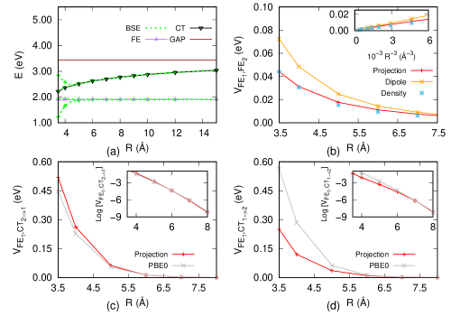
Figure 3: Results of the projective diabatization method for a pentacene dimer in PCM ($\epsilon_{r}=3.5$) as a function of the inter-fragment distance $R$. Results are presented in Figure 2 for the same system in the gas phase. The main differences introduced by PCM embedding are the 1.6 eV reduction of the gap due to screening phenomena and the stabilization of diabatic CT states in panel a. The magnitude of FE-FE couplings (panel b) is also reduced by dielectric screening.

The FE-FE coupling (Figure 3b) obtained with the diabatization scheme closely matches the value computed as screened interaction between transition densities (Equation 18), recovering the screened dipolar approximation at large $R$. The coupling between FEs in PCM is significantly reduced by screening phenomena as compared to gas-phase values. Figure 4 shows the effective screening factor, corresponding to the ratio between screened and unscreened Coulomb interaction between transition densities (see Equation 19), as a function of $R$. The screening factor decays monotonically from $\sim$0.7 at 4 Å distance to reach an asymptotic value of $\sim$0.55 at large $R$. The trend is similar to what was reported by Mennucci and coworkers for a large set of chromophores in PCM.^{93, 94} We further note that the limiting $s$ values is within 12% from the analytical result for point dipoles in spherical cavities (Equation 20), i.e. $s=0.492$ for $\epsilon_{\mathrm{opt}}=3.5$ (horizontal line in Figure 4). Such reasonable agreement shall be considered accidental, since for anisotropic cavities, the screening factor largely depends on the dipole orientation (see SI, Figure S1).

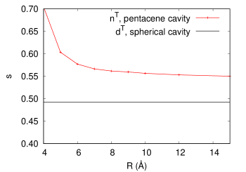
Figure 4: Effective screening factor $s$ (Equation 19) as a function of the intermolecular distance $R$. The red points are computed from the unscreened and PCM-screened interactions between the BSE transition densities ($n^{\mathrm{T}}$) of pentacene dimers. The black horizontal line marks the limit expected for point transition dipoles ($\mathbf{d}^{\mathrm{T}}$) in spherical cavities at large $R$ for $\varepsilon_{\mathrm{opt}}=3.5$ (Equation 20).

As for the FE-CT couplings (see Figure 3c,d), we observe an exponential decay of these couplings similar to the gas-phase result. The quality of the one-electron approximation (PBE0 couplings) is comparable to what obtained in the absence of PCM embedding. Also in the case of PCM, the direct coupling between CT states is negligible for $R>5$ Å.

3.2 Pentacene molecular crystal

We now apply our projective diabatization scheme to the pentacene crystal, which allows us to discuss some important and often overlooked aspects of the ab initio calculation of the parameters entering model Hamiltonians for extended systems. Before proceeding, we recall two technical aspects of our calculations that will be crucial for the quality of the results presented in the following. First, all calculations in the crystal employed a QM/MM scheme employing a polarizable atomistic model in the ground-state DFT calculation, where the chosen QM region (single molecule, dimer, etc.) is embedded in the electrostatic potential of the bulk crystal. The environmental screening of electronic excitations at the $GW$ and BSE level has been described at the PCM level ($\epsilon_{r}=3.5$, see Section 2.2 for details). The proper account of the electrostatic landscape and dielectric screening of the environment is essential for the reliable transfer of the parameters calculated from a small QM subsystem to crystals. In the second instance, the definition of the localized (diabatic) basis functions relies on a single (DFT, $GW$, BSE) calculation for each of the symmetry-unique molecules in the unit cell. Translational invariance is enforced by creating translational copies of unique fragments and defining the basis functions accordingly. This ensures phase consistency among all basis FE and CT states throughout a virtually infinite crystal, hence determining unambiguously the signs of the off-diagonal elements in model Hamiltonians.^{104, 3}

The pentacene crystal contains two symmetry-unique molecules in the unit cell arranged in a herringbone pattern (see Figure 5(a)). Two possible choices for molecular dimers to be chosen as QM subsystems are the herringbone ({1,2}, shown in Figure 5(a)a) and the parallel ({1,3}, Figure 5(a)b) dimers. Consistent with Section 3.1, the basis for pentacene dimers includes two FEs and two CT states (intermolecular HOMO$\to$LUMO transitions). For these two dimers, our projective scheme yields the two effective Hamiltonians:

$${\bf H}_{\mathrm{\{1,2\}}}=\ \ \NiceArray{rrrrl}\mathrm{FE}_{1}&\mathrm{FE}_{2}\mathrm{CT}_{1\to 2}\mathrm{CT}_{2\to 1}\\ 2.013-0.005-0.0570.099\mathrm{FE}_{1}\\ 1.9060.104-0.058\mathrm{FE}_{2}\\ 2.414-0.003\mathrm{CT}_{1\to 2}\\ 2.295\mathrm{CT}_{2\to 1}\\ \CodeAfter\SubMatrix({2-1}{5-4})$$ (23)

and

$${\bf H}_{\mathrm{\{1,3\}}}=\ \ \NiceArray{rrrrl}\mathrm{FE}_{1}&\mathrm{FE}_{3}\mathrm{CT}_{1\to 3}\mathrm{CT}_{3\to 1}\\ 2.002-0.012-0.026-0.048\mathrm{FE}_{1}\\ 2.002-0.048-0.026\mathrm{FE}_{3}\\ 2.5060.001\mathrm{CT}_{1\to 3}\\ 2.508\mathrm{CT}_{3\to 1}\\ \CodeAfter\SubMatrix({2-1}{5-4})$$ (24)

(a)

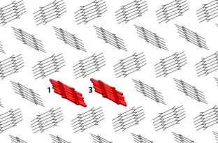
(b)

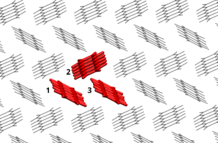
(d)

Figure 5: Rendering of the pentacene crystal, highlighting in red the (a,b) dimers and (c,d) trimers employed as QM subsystem in BSE QM/MM calculations. Molecules drawn in black correspond to the MM embedding environment. The blue frame in panel (a) displays the crystal unit cell. The numbering of molecular fragments will be used to label the basis functions used to set up the excitonic model.

aaaaaaaaaaaaaaaaaaa
aaaaaaaaaaaaaaaaaaa

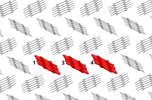
(c)

It would be tempting to use these Hamiltonian matrix elements obtained from these and other nearest-neighbor dimers to build the crystal Hamiltonian. However, some CT-CT couplings corresponding to charge hopping between nearest-neighbor fragments (i.e. those where the geminate charge sits on a third molecule, labeled HT and ET in Figure 1) cannot be obtained from dimer calculations. For instance, the direct coupling between CT_1→2 and CT_1→3 is not accessible from the two previous dimer calculations. This is an ET process that can be approximated as the LUMO-LUMO interaction among the fragment’s Kohn-Sham orbitals (i.e. $\langle\phi^{2}_{L}|\widehat{\textrm{H}}_{KS}|\phi^{3}_{L}\rangle$), for which we would expect a magnitude comparable to FE-CT couplings.

Trimer calculations have been thus performed to include these effects, specifically computing the $\{1,2,3\}$ and $\{1,3,4\}$ systems as defined in Figure 5(a)c,d. The construction of the diabatic basis for trimers follows the same prescription adopted for dimers, including 3 FEs and 6 CT states, resulting in a 9-state model. The values of all matrix elements are reported in the SI, the following discussion focuses on the most relevant ones.

As expected, ET and HT couplings are sizeable, with a magnitude of tens of meV. The comparison of the Hamiltonian obtained for the two trimers reveals that the et coupling is almost independent of the position of the hole, namely $\langle\mathrm{CT}_{2\to 1}|\mathrm{H}_{\{123\}}|\mathrm{CT}_{2\to 3}\rangle=-24$ meV and $\langle\mathrm{CT}_{4\to 1}|\mathrm{H}_{\{234\}}|\mathrm{CT}_{4\to 3}\rangle=-23$ meV. Similarly, also HT is almost unaffected by the electron position, i.e. $\langle\mathrm{CT}_{1\to 2}|\mathrm{H}_{\{123\}}|\mathrm{CT}_{3\to 2}\rangle=-48$ meV and $\langle\mathrm{CT}_{1\to 4}|\mathrm{H}_{\{134\}}|\mathrm{CT}_{3\to 4}\rangle=-49$ meV. The fact that these hopping terms barely depend on the position of the geminate charge, indicates that the screened-Coulomb ($W$) and exchange $v$ terms in the BSE Hamiltonian (see Equation 4) are almost negligible, as somewhat expected for loosely overlapping orbitals localized on different molecules. We note that these two HT and ET couplings are similar to their one-body approximation, $\langle\phi^{1}_{\mathrm{HOMO}}|\widehat{\textrm{HOMO}}_{KS}|\phi^{3}_{\mathrm{H}}\rangle=-29$ meV and $\langle\phi^{1}_{\mathrm{LUMO}}|\widehat{\textrm{H}}_{KS}|\phi^{3}_{\mathrm{LUMO}}\rangle=-65$ meV for HT and ET, respectively. However, the quantitative discrepancy between these Kohn-Sham and BSE/$GW$ couplings attests to the importance of many-body effects for these interactions.

By performing the diabatization on different embedded dimers and trimers from the pentacene crystal structure, we recognize the presence of some diagonal and off-diagonal matrix elements that can be obtained from multiple calculations, which are reported in Table 1. The diagonal energy of the FE of fragment 1 is the only parameter that is accessible in all calculations. Its variability is below 30 meV, which corresponds to 1.5% of the excitation energy. A smaller fluctuation among different choices of the QM region is obtained for the energy of the FE of fragment 3.

The diagonal energies of CT states are the parameters that are mostly sensitive to the environment, as they consist of localized charges (in contrast with FE that are neutral species) that directly probe the local electrostatic potential within the crystal, and that experience the response of the polarizable medium to their strong dipole field. The largest variability is found for the energy of CT_1→3, i.e. 47 meV, below 2% of the excitation energy. This is a very positive result, being this variability smaller than the accuracy of the BSE/$GW$-based QM/MM methodology (typically 0.1-0.2 eV). For comparison, calculation not accounting for any embedding (i.e. computing dimers and trimers in the gas phase), yields CT states whose energy varies in the range of 0.48 eV, one order of magnitude larger than embedded calculations. We note that most of the spread is cured by the electrostatic embedding in the ground state, which compensates for the otherwise different electrostatic fields at molecular sites developing in gas-phase dimers and trimers. Polarization effects on excitations further reduce the spread in CT states energies obtained from calculations on different QM subsystems and, most importantly, are crucial to reproduce excitation energies in a condensed phase correctly. The spread in the values obtained for off-diagonal matrix elements is found to be smaller than 1 meV, as shown in Table 2.

In general, electrostatic and dielectric embedding are found to be key ingredients for the transferability of the parameters from BSE QM/MM calculations on small embedded molecular clusters to crystals. A proper embedding ensures the stability of the matrix elements derived from our projective diabatization scheme against the arbitrary choice of the QM subsystem, as is demonstrated here in the paradigmatic case of the pentacene crystal. This attests to the robustness and internal consistency of our approach.

	$\{1,2\}$	$\{1,3\}$	$\{1,2,3\}$	$\{1,3,4\}$
$\langle\mathrm{FE}_{1}|\mathrm{H}|\mathrm{FE}_{1}\rangle$	2.013	2.002	2.031	2.019
$\langle\mathrm{FE}_{3}|\mathrm{H}|\mathrm{FE}_{3}\rangle$		2.002	2.005	2.002
$\langle\mathrm{CT}_{1\to 3}|\mathrm{H}|\mathrm{CT}_{1\to 3}\rangle$		2.506	2.553	2.526
$\langle\mathrm{CT}_{3\to 1}|\mathrm{H}|\mathrm{CT}_{3\to 1}\rangle$		2.509	2.501	2.514
$\langle\mathrm{FE}_{1}|\mathrm{H}|\mathrm{FE}_{3}\rangle$		$-0.012$	$-0.013$	$-0.012$
$\langle\mathrm{FE}_{1}|\mathrm{H}|\mathrm{CT}_{1\to 3}\rangle$		$-0.026$	$-0.024$	$-0.026$
$\langle\mathrm{FE}_{1}|\mathrm{H}|\mathrm{CT}_{3\to 1}\rangle$		$-0.048$	$-0.048$	$-0.048$
$\langle\mathrm{FE}_{3}|\mathrm{H}|\mathrm{CT}_{1\to 3}\rangle$		$-0.048$	$-0.048$	$-0.048$
$\langle\mathrm{FE}_{3}|\mathrm{H}|\mathrm{CT}_{3\to 1}\rangle$		$-0.026$	$-0.025$	$-0.026$

Table 1: Excitonic model matrix elements (in eV) for the pentacene crystal obtained with the projective diabatization scheme based on embedded BSE calculations (QM/MM). For a given matrix element, we report the values obtained from calculations performed on different dimers and trimers as QM systems. The remarkable stability of these energies as obtained from different calculations testifies to the quality and consistency of the method.

As a final illustration of the quality of the excitonic models that can be built with the present diabatization scheme, we consider the case of a pentacene tetramer embedded in the crystal structure (fragments $\{1,2,3,4\}$ as defined in Figure 5(a)). This represents a fairly large system that can be computed as a whole with embedded BSE calculations. The corresponding transition energies, shown in the left column of Table 2, serve as a reference for the eigenvalues of the excitonic model Hamiltonian. The latter has been assembled in a modular fashion with matrix elements obtained from calculations on molecular trimers (see SI). The exciton energies obtained with the model (right column in Table 2) are in excellent agreement with reference BSE ones. This is especially true in the low-energy region the model is designed for, with an absolute difference within 11 meV for the first 8 excitons. The agreement progressively worsens at higher energies, up to reach 88 meV for the highest-energy state in Table 2. This is consistent with the fact that the assumption of the model breaks down as we move to higher energies, where excitation manifolds become more and more dense and the chosen minimal basis becomes insufficient to describe the corresponding states. Such an overall excellent result for the embedded pentacene tetramer, together with the successful consistency checks on equivalent matrix elements derived from different calculations, demonstrate the quality of our BSE-based projective diabatization scheme and its potential for application in future studies.

BSE	Model Hamiltonian
1.842	1.844
1.943	1.954
2.003	1.993
2.021	2.018
2.248	2.252
2.370	2.371
2.382	2.386
2.415	2.414
2.460	2.510
2.507	2.531
2.587	2.589
2.660	2.653
2.680	n.a.
2.698	n.a.
2.871	2.822
2.915	2.827

Table 2: Comparison between the BSE excitation energies (in eV) for the pentacene $\{1,2,3,4\}$ tetramer embedded in the crystal, and those obtained with the model Hamiltonian. The latter does not include the states CT_2→4 and CT_4→2 in the basis so two excitons are not available (n.a.) within the model.

4 Conclusions

In this work, we have presented a general and versatile approach to building effective excitonic models from ab initio many-body calculations, namely the $GW$ and the BSE Green’s function formalisms. The derived excitonic models inherit the ability of BSE/$GW$ to accurately describe FE and CT excitations, thanks to the explicit account of non-local electronic correlations and especially the excitonic e-h interaction. The combination of BSE/$GW$ formalisms with an effective description of the embedding environment in a QM/MM framework, grants access to excitonic models for condensed-phase systems. The merits of our BSE-based diabatization scheme have been illustrated and validated through specific examples of model molecular dimers and a molecular crystal, taking pentacene as a paradigmatic test case.

The proposed multi-state projective diabatization scheme starts from the definition of basis functions (FEs localized on single fragments and inter-fragment CT states) and derives the corresponding excitonic Hamiltonian in order to match target exciton energies and wavefunctions from BSE. It is worth recalling some important distinctive aspects of the methodology: (i) It preserves the non-orthogonality of the basis (usually neglected in excitonic models) that is an essential requisite for upscaling the model to larger systems; (ii) It naturally ensures consistent phase relationships between the excitonic basis on translationally-equivalent molecules, which is necessary for the correct description of the photophysical properties of molecular crystals (e.g. exciton dispersion, quantum dynamics); (iii) It accounts for electrostatic and dielectric embedding, leading to model parameters that are explicitly calculated for a condensed phase and that minimally depend on the arbitrary choice of the QM subsystem (QM/MM partitioning). The combination of these features allows one to derive exciton energies and couplings in the diabatic representation that are computed for relatively small QM systems (molecular dimers or trimers) and that can be readily transferred to model Hamiltonians for extended systems, achieving an accuracy comparable to the original BSE calculation.

The proposed projective diabatization scheme paves the way for an accurate, insightful, and computationally-efficient description of the excited states of molecular solids based on many-body ab initio theories, setting solid grounds for future studies on complex systems of timely interest.

G.D. acknowledges the contribution from Jing Li in the first steps of this research and thanks Samuele Giannini for stimulating discussions. This work received financial support from the French ”Agence Nationale de la Recherche”, project RAPTORS (ANR-21-CE24-0004-01). This work was performed using HPC resources from GENCI-TGCC (Grant No. 2021-A0110910016).

Appendix A Appendix: Interaction of two dipoles inside separated spherical cavities

A.1 The cavity response to an interior point multipole

In the following, we consider a continuous polarizable medium with a dielectric constant $\epsilon$ . Let us start placing the center of a cavity of radius $a$ as the origin and setting the position of a point charge $q$ at $(r,\theta,\phi)=(b,0,0)$. This corresponds to a standard electrostatic problem which is solved by considering first that in the absence of the cavity, the potential due to the point charge $q$ can be expressed using Legendre polynomials of integer order $P_{n}$

$$V_{q}(r,\theta,\phi)=\left\{\begin{array}[]{lr}\cfrac{1}{\epsilon_{0}}\displaystyle\sum_{n=0}\cfrac{q}{b}\left(\cfrac{r}{b}\right)^{n}P_{n}(\cos\theta)&(r<b)\\ \cfrac{1}{\epsilon_{0}}\displaystyle\sum_{n=0}\cfrac{q}{r}\left(\cfrac{b}{r}\right)^{n}P_{n}(\cos\theta)&(r>b)\\ \end{array}\right.$$ (25)

with $\epsilon_{0}$ being the vacuum permittivity. In our case, we simply generalize this definition to (non-normed) point multipoles by differentiating the formulas with respect to $b$

$$V_{l}(r,\theta,\phi)=\cfrac{d^{l}}{db^{l}}V_{q}(r,\theta,\phi)=\left\{\begin{array}[]{lr}\cfrac{1}{\epsilon_{0}}\displaystyle\sum_{n=0}(-1)^{l}\cfrac{(n+l)!}{n!}\cfrac{q}{b^{l+1}}\left(\cfrac{r}{b}\right)^{n}P_{n}(\cos\theta)&(r<b)\\ \cfrac{1}{\epsilon_{0}}\displaystyle\sum_{n=0}\cfrac{(n+l)!}{n!}\cfrac{q}{r^{l+1}}\left(\cfrac{b}{r}\right)^{n}P_{n+l}(\cos\theta)&(r>b).\\ \end{array}\right.$$ (26)

In particular, the term $n=0$ defines the potential and normal field due to the multipole in the long-range limit $b/r\to 0$

$$V_{l}(r,\theta,\phi) \stackrel{{\scriptstyle\frac{b}{r}\to 0}}{{=}} \cfrac{l!}{\epsilon_{0}}\,\cfrac{q}{r^{l+1}}P_{l}(\cos\theta)$$ (27)

$$\cfrac{d}{dr}V_{l}(r,\theta,\phi) \stackrel{{\scriptstyle\frac{b}{r}\to 0}}{{=}} -\cfrac{(l+1)!}{\epsilon_{0}}\,\cfrac{q}{r^{l+2}}P_{l}(\cos\theta)$$ (28)

Similarly, the reaction field from the cavity can be written in the general form

$$V_{C}(r,\theta,\phi)=\left\{\begin{array}[]{lr}\displaystyle\sum_{n=0}A_{n}\left(\cfrac{r}{a}\right)^{n}P_{n}(\cos\theta)&(r<a)\\ \displaystyle\sum_{n=0}A_{n}\left(\cfrac{a}{r}\right)^{n+1}\!\!P_{n}(\cos\theta)&(r>a)\\ \end{array}\right.$$ (29)

with the derivatives along $r$

$$\cfrac{d}{dr}V_{C}(r,\theta,\phi)=\left\{\begin{array}[]{lr}\displaystyle\sum_{n=0}n\cfrac{A_{n}}{r}\left(\cfrac{r}{a}\right)^{n}P_{n}(\cos\theta)&(r<a)\\ \displaystyle\sum_{n=0}(n+1)\cfrac{-aA_{n}}{r^{2}}\left(\cfrac{a}{r}\right)^{n}\!\!P_{n}(\cos\theta)&(r>a).\\ \end{array}\right.$$ (30)

The coefficients $A_{n}$ can then be evaluated by noting that the radial component of the total electric displacement field $D=\epsilon E$ is continuous across the cavity boundary at r = a

$$\epsilon_{0}\left.\cfrac{d}{dr}(V_{l}+V_{c})\;\right]_{a^{-}}=\epsilon\left.\cfrac{d}{dr}(V_{l}+V_{c})\;\right]_{a^{+}},$$ (31)

which leads in particular to (sorting out the $P_{n\neq l}(\cos\theta)$ factors)

$$A_{l}=\cfrac{q}{\epsilon_{0}\,a^{l+1}}\cfrac{(\epsilon_{0}-\epsilon)(l+1)!}{(\epsilon_{0}+\epsilon)(l+1)-\epsilon_{0}}.$$ (32)

Thence, the resulting general long-range limit for the renormalization of the potential outside a spherical cavity, for a multipole placed within the cavity:

$$\begin{split}\cfrac{[V_{l}+V_{C}](r,\theta,\phi)}{V_{q}(r,\theta,\phi)}\;\stackrel{{\scriptstyle\frac{b}{r}\to 0}}{{=}}\;\cfrac{(2l+1)\epsilon_{0}}{(\epsilon_{0}+\epsilon)l+\epsilon}\end{split}$$ (33)

Introducing the relative permittivity $\epsilon_{r}=\epsilon/\epsilon_{0}$, we recover the usual charge potential reaction field renormalization for $l=0$,

$$\cfrac{[V_{q}+V_{C}](r,\theta,\phi)}{V_{q}(r,\theta,\phi)}\;\stackrel{{\scriptstyle\frac{b}{r}\to 0}}{{=}}\;\cfrac{1}{\epsilon_{r}}$$ (34)

while for $l=1$ we recover the corresponding expression for a dipole distribution $d$

$$\cfrac{[V_{d}+V_{C}](r,\theta,\phi)}{V_{d}(r,\theta,\phi)}\;\stackrel{{\scriptstyle\frac{b}{r}\to 0}}{{=}}\;\cfrac{3}{1+2\epsilon_{r}}.$$ (35)

A.2 The cavity response to an exterior field

We consider now a homogeneous electric field $E$ (along the x coordinate) so that the potential reads

$$V_{ext}(r,\theta,\phi)=V_{0}+r\,E\,P_{1}(\cos\theta)$$ (36)

(here we simply used the fact that $P_{1}(x)=x$). Once again, we write the reaction field from the cavity and its derivative using equations (29) and (30) and evaluate the coefficients $A_{n}$ by noting that the radial component of the total electric displacement field $D=\epsilon E$ is continuous across the boundary r = a

$$\epsilon_{0}\left.\cfrac{d}{dr}(V_{ext}+V_{C})\;\right]_{a^{-}}=\epsilon\left.\cfrac{d}{dr}(V_{ext}+V_{C})\;\right]_{a^{+}},$$ (37)

which brings immediately

$$A_{1}=-a\,E\,\cfrac{\epsilon_{0}-\epsilon}{\epsilon_{0}+2\epsilon}\;,\quad A_{n\neq 1}=0$$ (38)

with the corresponding cavity reaction potential

$$V_{C}(r,\theta,\phi)=\left\{\begin{array}[]{lr}\cfrac{\epsilon-\epsilon_{0}}{\epsilon_{0}+2\epsilon}\,r\,E\,P_{1}(\cos\theta)&(r<a)\\ \cfrac{\epsilon-\epsilon_{0}}{\epsilon_{0}+2\epsilon}\,E\,\cfrac{a^{3}}{r^{2}}\,P_{1}(\cos\theta)&(r>a)\\ \end{array}\right.$$ (39)

so that the total potential seen from within the cavity is

$$\left[V_{ext}+V_{C}\right](r,\theta,\phi)=V_{0}+\left(1+\cfrac{\epsilon-\epsilon_{0}}{\epsilon_{0}+2\epsilon}\right)\,r\,E\,P_{1}(\cos\theta).$$ (40)

Here, we get the relation between the total electric field seen from within the cavity and the applied external field

$$\cfrac{d}{dr}\left[V_{ext}+V_{C}\right](r,\theta,\phi)=\frac{3\varepsilon}{\varepsilon_{0}+2\varepsilon}E$$ (41)

which is the Onsager result for the cavity field.⁹⁵

A.3 The dipole-dipole interaction across separate cavities

In this case, we combine results from the previous sections. The dipoles ${\bf d}$ within cavity 1 centered in ${\bf R}=(0,0,R_{z})$ generates a screened potential outside its cavity that was derived in the previous sections

$$V_{d}({\bf r})=\cfrac{3}{\epsilon_{0}+2\epsilon}\,\cfrac{{\bf d}\cdot({\bf r}-{\bf R})}{|{{\bf r}-{\bf R}}|^{3}}.$$ (42)

The resulting electric field reads

$$E_{d}({\bf r})=\cfrac{3}{\epsilon_{0}+2\epsilon}\left(3\,\cfrac{{\bf d}\cdot({\bf r}-{\bf R})}{|{{\bf r}-{\bf R}}|^{5}}\,({\bf r}-{\bf R})-\cfrac{{\bf d}}{|{{\bf r}-{\bf R}}|^{3}}\right)$$ (43)

so that in the vicinity of the second cavity placed at the origin $(0,0,0)$, the potential can be expanded as

$$V_{d}({\bf r})=V_{d}(0)+{\bf r}\cdot E_{d}(0)+\dots\\$$ (44)

with

$$V_{d}(0)=\cfrac{3}{\epsilon_{0}+2\epsilon}\,\cfrac{d_{z}}{R_{z}^{2}}$$ (45)

and

$$E_{d}(0)=\cfrac{3}{\epsilon_{0}+2\epsilon}\,\cfrac{(-d_{x},-d_{y},2d_{z})}{R_{z}^{3}}$$ (46)

Applying the result (40) from the previous section, we get that the total potential $V$, as seen from a charge distribution placed within the second cavity reads

$$\begin{split}V({\bf r})=&V_{d}(0)+\left(1+\cfrac{\epsilon-\epsilon_{0}}{\epsilon_{0}+2\epsilon}\right){\bf r}\cdot E_{d}(0)+\dots\\ &=\cfrac{3}{\epsilon_{0}+2\epsilon}\,\cfrac{d_{z}}{R_{z}^{2}}+\epsilon\left(\cfrac{3}{\epsilon_{0}+2\epsilon}\right)^{2}\,\cfrac{{\bf r}\cdot(-d_{x},-d_{y},2d_{z})}{R_{z}^{3}}.\end{split}$$ (47)

A charge placed in the second cavity will thus probe the first term of (47) right-hand side, leading to a charge-dipole interaction renormalized by

$$\cfrac{3}{1+2\epsilon_{r}}$$ (48)

while a dipole placed in the second cavity will only probe the second term of (47) right-hand side, leading to a dipole-dipole interaction renormalized by

$$\epsilon_{r}\left(\frac{3}{1+2\epsilon_{r}}\right)^{2}$$ (49)

TOC Graphics

References

- Scholes and Rumbles 2006 Scholes, G. D.; Rumbles, G. Excitons in nanoscale systems. Nature Mater. 2006, 5, 683–696
- Brédas et al. 2009 Brédas, J.-L.; Norton, J. E.; Cornil, J.; Coropceanu, V. Molecular Understanding of Organic Solar Cells: The Challenges. Accounts of Chemical Research 2009, 42, 1691–1699, PMID: 19653630
- Hestand and Spano 2018 Hestand, N. J.; Spano, F. C. Expanded Theory of H- and J-Molecular Aggregates: The Effects of Vibronic Coupling and Intermolecular Charge Transfer. Chem. Rev. 2018, 118, 7069–7163, PMID: 29664617
- Dimitriev 2022 Dimitriev, O. P. Dynamics of Excitons in Conjugated Molecules and Organic Semiconductor Systems. Chem. Rev. 2022, 122, 8487–8593, PMID: 35298145
- Casida 1995 Casida, M. E. Recent Advances in Density Functional Methods; 1995; pp 155–192
- Prlj et al. 2015 Prlj, A.; Curchod, B. F. E.; Fabrizio, A.; Floryan, L.; Corminboeuf, C. Qualitatively Incorrect Features in the TDDFT Spectrum of Thiophene-Based Compounds. J. Phys. Chem. Lett. 2015, 6, 13–21, PMID: 26263085
- Stein et al. 2009 Stein, T.; Kronik, L.; Baer, R. Reliable Prediction of Charge Transfer Excitations in Molecular Complexes Using Time-Dependent Density Functional Theory. J. Am. Chem. Soc. 2009, 131, 2818–2820, PMID: 19239266
- Dreuw and Head-Gordon 2004 Dreuw, A.; Head-Gordon, M. Failure of time-dependent density functional theory for long-range charge-transfer excited states: the zincbacteriochlorin-bacteriochlorin and bacteriochlorophyll-spheroidene complexes. J. Am. Chem. Soc. 2004, 126, 4007–4016
- Yanai et al. 2004 Yanai, T.; Tew, D. P.; Handy, N. C. A new hybrid exchange–correlation functional using the Coulomb-attenuating method (CAM-B3LYP). Chem. Phys. Lett. 2004, 393, 51–57
- Baer et al. 2010 Baer, R.; Livshits, E.; Salzner, U. Tuned Range-Separated Hybrids in Density Functional Theory. Annu. Rev. Phys. Chem. 2010, 61, 85–109
- Hedin 1965 Hedin, L. New Method for Calculating the One-Particle Green’s Function with Application to the Electron-Gas Problem. Phys. Rev. 1965, 139, A796–A823
- Strinati et al. 1980 Strinati, G.; Mattausch, H. J.; Hanke, W. Dynamical Correlation Effects on the Quasiparticle Bloch States of a Covalent Crystal. Phys. Rev. Lett. 1980, 45, 290–294
- Hybertsen and Louie 1986 Hybertsen, M. S.; Louie, S. G. Electron correlation in semiconductors and insulators: Band gaps and quasiparticle energies. Phys. Rev. B 1986, 34, 5390–5413
- Onida et al. 2002 Onida, G.; Reining, L.; Rubio, A. Electronic excitations: density-functional versus many-body Green’s-function approaches. Rev. Mod. Phys. 2002, 74, 601–659
- Martin et al. 2016 Martin, R.; Reining, L.; Ceperley, D. Interacting Electrons: Theory and Computational Approaches; Cambridge University Press, 2016
- Golze et al. 2019 Golze, D.; Dvorak, M.; Rinke, P. The GW Compendium: A Practical Guide to Theoretical Photoemission Spectroscopy. Front. Chem. 2019, 7, 377
- Strinati 1988 Strinati, G. Application of the Green’s functions method to the study of the optical properties of semiconductors. La Rivista del Nuovo Cimento (1978-1999) 1988, 11, 1
- Salpeter and Bethe 1951 Salpeter, E. E.; Bethe, H. A. A Relativistic Equation for Bound-State Problems. Phys. Rev. 1951, 84, 1232–1242
- Sham and Rice 1966 Sham, L. J.; Rice, T. M. Many-Particle Derivation of the Effective-Mass Equation for the Wannier Exciton. Phys. Rev. 1966, 144, 708–714
- Hanke and Sham 1979 Hanke, W.; Sham, L. J. Many-Particle Effects in the Optical Excitations of a Semiconductor. Phys. Rev. Lett. 1979, 43, 387–390
- Rostgaard et al. 2010 Rostgaard, C.; Jacobsen, K. W.; Thygesen, K. S. Fully self-consistent GW calculations for molecules. Phys. Rev. B 2010, 81, 085103
- Kaczmarski et al. 2010 Kaczmarski, M. S.; Ma, Y.; Rohlfing, M. Diabatic states of a photoexcited retinal chromophore from ab initio many-body perturbation theory. Phys. Rev. B 2010, 81, 115433
- Blase et al. 2011 Blase, X.; Attaccalite, C.; Olevano, V. First-principles calculations for fullerenes, porphyrins, phtalocyanine, and other molecules of interest for organic photovoltaic applications. Phys. Rev. B 2011, 83, 115103
- Blase and Attaccalite 2011 Blase, X.; Attaccalite, C. Charge-transfer excitations in molecular donor-acceptor complexes within the many-body Bethe-Salpeter approach. Appl. Phys. Lett. 2011, 99, 171909
- Baumeier et al. 2012 Baumeier, B.; Andrienko, D.; Ma, Y.; Rohlfing, M. Excited States of Dicyanovinyl-Substituted Oligothiophenes from Many-Body Green’s Functions Theory. J. Chem. Theory Comput. 2012, 8, 997–1002, PMID: 26593361
- Marom et al. 2012 Marom, N.; Caruso, F.; Ren, X.; Hofmann, O. T.; Körzdörfer, T.; Chelikowsky, J. R.; Rubio, A.; Scheffler, M.; Rinke, P. Benchmark of methods for azabenzenes. Phys. Rev. B 2012, 86, 245127
- Duchemin et al. 2012 Duchemin, I.; Deutsch, T.; Blase, X. Short-Range to Long-Range Charge-Transfer Excitations in the Zincbacteriochlorin-Bacteriochlorin Complex: A Bethe-Salpeter Study. Phys. Rev. Lett. 2012, 109, 167801
- Bruneval and Marques 2013 Bruneval, F.; Marques, M. Benchmarking the starting points of the GW approximation for molecules. Journal of chemical theory and computation 2013, 9, 324
- van Setten et al. 2013 van Setten, M. J.; Weigend, F.; Evers, F. The GW-Method for Quantum Chemistry Applications: Theory and Implementation. J. Chem. Theory Comput. 2013, 9, 232–246
- Baumeier et al. 2014 Baumeier, B.; Rohlfing, M.; Andrienko, D. Electronic Excitations in Push–Pull Oligomers and Their Complexes with Fullerene from Many-Body Green’s Functions Theory with Polarizable Embedding. J. Chem. Theory Comput. 2014, 10, 3104–3110
- Blase et al. 2018 Blase, X.; Duchemin, I.; Jacquemin, D. The Bethe–Salpeter equation in chemistry: relations with TD-DFT, applications and challenges. Chem. Soc. Rev. 2018, 47, 1022–1043
- Faber et al. 2011 Faber, C.; Attaccalite, C.; Olevano, V.; Runge, E.; Blase, X. First-principles calculations for DNA and RNA nucleobases. Phys. Rev. B 2011, 83, 115123
- van Setten et al. 2015 van Setten, M. J.; Caruso, F.; Sharifzadeh, S.; Ren, X.; Scheffler, M.; Liu, F.; Lischner, J.; Lin, L.; Deslippe, J. R.; Louie, S. G.; Yang, C.; Weigend, F.; Neaton, J. B.; Evers, F.; Rinke, P. GW100: Benchmarking G0W0 for Molecular Systems. J. Chem. Theory Comput. 2015, 11, 5665–5687
- Jacquemin et al. 2015 Jacquemin, D.; Duchemin, I.; Blase, X. Benchmarking the Bethe-Salpeter Formalism on a Standard Organic Molecular Set. J. Chem. Theory Comput. 2015, 11, 3290–3304
- Jacquemin et al. 2015 Jacquemin, D.; Duchemin, I.; Blase, X. 0-0 Energies Using Hybrid Schemes: Benchmarks of TD-DFT, CIS(D), ADC(2), CC2, and BSE/GW formalisms for 80 Real-Life Compounds. J. Chem. Theory Comput. 2015, 11, 5340–5359
- Bruneval et al. 2015 Bruneval, F.; Hamed, S. M.; Neaton, J. B. A systematic benchmark of the ab initio Bethe-Salpeter equation approach for low-lying optical excitations of small organic molecules. The Journal of Chemical Physics 2015, 142
- Knight et al. 2016 Knight, J. W.; Wang, X.; Gallandi, L.; Dolgounitcheva, O.; Ren, X.; Ortiz, J. V.; Rinke, P.; Körzdörfer, T.; Marom, N. Accurate Ionization Potentials and Electron Affinities of Acceptor Molecules III: A Benchmark of GW Methods. J. Chem. Theory Comput. 2016, 12, 615–626, PMID: 26731609
- Kaplan et al. 2016 Kaplan, F.; Harding, M. E.; Seiler, C.; Weigend, F.; Evers, F.; van Setten, M. J. Quasi-Particle Self-Consistent GW for Molecules. J. Chem. Theory Comput. 2016, 12, 2528–2541, PMID: 27168352
- Rangel et al. 2016 Rangel, T.; Hamed, S. M.; Bruneval, F.; Neaton, J. B. Evaluating the GW Approximation with CCSD(T) for Charged Excitations Across the Oligoacenes. J. Chem. Theory Comput. 2016, 12, 2834–2842, PMID: 27123935
- Rangel et al. 2017 Rangel, T.; Hamed, S. M.; Bruneval, F.; Neaton, J. B. An assessment of low-lying excitation energies and triplet instabilities of organic molecules with an ab initio Bethe-Salpeter equation approach and the Tamm-Dancoff approximation. The Journal of Chemical Physics 2017, 146, 194108
- Gui et al. 2018 Gui, X.; Holzer, C.; Klopper, W. Accuracy Assessment of GW Starting Points for Calculating Molecular Excitation Energies Using the Bethe–Salpeter Formalism. J. Chem. Theory Comput. 2018, 14, 2127–2136, PMID: 29499116
- Liu et al. 2020 Liu, C.; Kloppenburg, J.; Yao, Y.; Ren, X.; Appel, H.; Kanai, Y.; Blum, V. All-electron ab initio Bethe-Salpeter equation approach to neutral excitations in molecules with numeric atom-centered orbitals. J. Chem. Phys. 2020, 152, 044105
- Förster and Visscher 2021 Förster, A.; Visscher, L. GW100: A Slater-Type Orbital Perspective. J. Chem. Theory Comput. 2021, 17, 5080–5097, PMID: 34236172
- Duchemin et al. 2016 Duchemin, I.; Jacquemin, D.; Blase, X. Combining the GW formalism with the polarizable continuum model: A state-specific non-equilibrium approach. J. Chem. Phys. 2016, 144, 164106
- Duchemin et al. 2018 Duchemin, I.; Guido, C. A.; Jacquemin, D.; Blase, X. The Bethe–Salpeter formalism with polarisable continuum embedding: Reconciling linear-response and state-specific features. Chemical science 2018, 9, 4430–4443
- Clary et al. 2023 Clary, J. M.; Del Ben, M.; Sundararaman, R.; Vigil-Fowler, D. Impact of solvation on the GW quasiparticle spectra of molecules. J. Appl. Phys. 2023, 134
- Kim et al. 2022 Kim, S.-J.; Lebègue, S.; Ringe, S.; Kim, H. GW quasiparticle energies and bandgaps of two-dimensional materials immersed in water. J. Phys. Chem. Lett. 2022, 13, 7574–7582
- Li et al. 2016 Li, J.; D’Avino, G.; Duchemin, I.; Beljonne, D.; Blase, X. Combining the Many-Body GW Formalism with Classical Polarizable Models: Insights on the Electronic Structure of Molecular Solids. J. Phys. Chem. Lett. 2016, 7, 2814–2820
- Li et al. 2018 Li, J.; D’Avino, G.; Duchemin, I.; Beljonne, D.; Blase, X. Accurate description of charged excitations in molecular solids from embedded many-body perturbation theory. Phys. Rev. B 2018, 97, 035108
- Amblard et al. 2023 Amblard, D.; Blase, X.; Duchemin, I. Many-body GW calculations with very large scale polarizable environments made affordable: A fully ab initio QM/QM approach. J. Chem. Phys. 2023, 159, 164107
- Amblard et al. 2024 Amblard, D.; Blase, X.; Duchemin, I. Static versus dynamically polarizable environments within the many-body GW formalism. J. Chem. Phys. 2024, 160, 154104
- Li et al. 2017 Li, J.; D’Avino, G.; Pershin, A.; Jacquemin, D.; Duchemin, I.; Beljonne, D.; Blase, X. Correlated electron-hole mechanism for molecular doping in organic semiconductors. Phys. Rev. Mater. 2017, 1, 025602
- Comin et al. 2022 Comin, M.; Lemaur, V.; Giunchi, A.; Beljonne, D.; Blase, X.; D’Avino, G. Doping of semicrystalline conjugated polymers: dopants within alkyl chains do it better. J. Mater. Chem. C 2022, 10, 13815–13825
- Kim et al. 2024 Kim, S.-J.; Lebègue, S.; Ringe, S.; Kim, H. Elucidating Solvatochromic Shifts in Two-Dimensional Photocatalysts by Solving the Bethe–Salpeter Equation Coupled with Implicit Solvation Method. J. Phys. Chem. Lett. 2024, 15, 4575–4580
- Wehner et al. 2018 Wehner, J.; Brombacher, L.; Brown, J.; Junghans, C.; Çaylak, O.; Khalak, Y.; Madhikar, P.; Tirimbò, G.; Baumeier, B. Electronic excitations in complex molecular environments: Many-body green’s functions theory in VOTCA-XTP. J. Chem. Theory Comput. 2018, 14, 6253–6268
- Dong et al. 2020 Dong, Y.; Nikolis, V. C.; Talnack, F.; Chin, Y.-C.; Benduhn, J.; Londi, G.; Kublitski, J.; Zheng, X.; Mannsfeld, S. C. B.; Spoltore, D.; Muccioli, L.; Li, J.; Blase, X.; Beljonne, D.; Kim, J.-S.; Bakulin, A. A.; D’Avino, G.; Durrant, J. R.; Vandewal, K. Orientation dependent molecular electrostatics drives efficient charge generation in homojunction organic solar cells. Nature Commun. 2020, 11, 4617
- Tiago et al. 2003 Tiago, M. L.; Northrup, J. E.; Louie, S. G. Ab initio calculation of the electronic and optical properties of solid pentacene. Phys. Rev. B 2003, 67, 115212
- Cudazzo et al. 2012 Cudazzo, P.; Gatti, M.; Rubio, A. Excitons in molecular crystals from first-principles many-body perturbation theory: Picene versus pentacene. Phys. Rev. B 2012, 86, 195307
- Cudazzo et al. 2013 Cudazzo, P.; Gatti, M.; Rubio, A.; Sottile, F. Frenkel versus charge-transfer exciton dispersion in molecular crystals. Phys. Rev. B 2013, 88, 195152
- Cocchi et al. 2018 Cocchi, C.; Breuer, T.; Witte, G.; Draxl, C. Polarized absorbance and Davydov splitting in bulk and thin-film pentacene polymorphs. Phys. Chem. Chem. Phys. 2018, 20, 29724–29736
- May and Kühn 2011 May, V.; Kühn, O. Charge and Energy Transfer Dynamics in Molecular Systems; John Wiley & Sons, 2011
- Yamagata et al. 2011 Yamagata, H.; Norton, J.; Hontz, E.; Olivier, Y.; Beljonne, D.; Brédas, J. L.; Silbey, R. J.; Spano, F. C. The nature of singlet excitons in oligoacene molecular crystals. J. Chem. Phys. 2011, 134, 204703
- Popp et al. 2021 Popp, W.; Brey, D.; Binder, R.; Burghardt, I. Quantum Dynamics of Exciton Transport and Dissociation in Multichromophoric Systems. Annu. Rev. Phys. Chem. 2021, 72, 591–616
- Tamura et al. 2011 Tamura, H.; Burghardt, I.; Tsukada, M. Exciton Dissociation at Thiophene/Fullerene Interfaces: The Electronic Structures and Quantum Dynamics. J. Phys. Chem. C 2011, 115, 10205–10210
- Giannini et al. 2022 Giannini, S.; Peng, W.-T.; Cupellini, L.; Padula, D.; Carof, A.; Blumberger, J. Exciton transport in molecular organic semiconductors boosted by transient quantum delocalization. Nature Comm. 2022, 13, 2755
- Hsu 2009 Hsu, C.-P. The Electronic Couplings in Electron Transfer and Excitation Energy Transfer. Acc. Chem. Res. 2009, 42, 509–518
- Madjet et al. 2006 Madjet, M. E.; Abdurahman, A.; Renger, T. Intermolecular Coulomb Couplings from Ab Initio Electrostatic Potentials: Application to Optical Transitions of Strongly Coupled Pigments in Photosynthetic Antennae and Reaction Centers. J. Phys. Chem. B 2006, 110, 17268–17281, PMID: 16928026
- Cave and Newton 1996 Cave, R. J.; Newton, M. D. Generalization of the Mulliken-Hush treatment for the calculation of electron transfer matrix elements. Chem. Phys. Lett. 1996, 249, 15–19
- Rust et al. 2002 Rust, M.; Lappe, J.; Cave, R. J. Multistate Effects in Calculations of the Electronic Coupling Element for Electron Transfer Using the Generalized Mulliken-Hush Method. J. Phys. Chem. A 2002, 106, 3930–3940
- Hsu et al. 2008 Hsu, C.-P.; You, Z.-Q.; Chen, H.-C. Characterization of the Short-Range Couplings in Excitation Energy Transfer. J. Phys. Chem. C 2008, 112, 1204–1212
- Subotnik et al. 2009 Subotnik, J. E.; Cave, R. J.; Steele, R. P.; Shenvi, N. The initial and final states of electron and energy transfer processes: Diabatization as motivated by system-solvent interactions. J. Chem. Phys. 2009, 130, 234102
- Difley and Van Voorhis 2011 Difley, S.; Van Voorhis, T. Exciton/Charge-Transfer Electronic Couplings in Organic Semiconductors. J. Chem. Theory Comput. 2011, 7, 594–601, PMID: 26596293
- Yang and Hsu 2013 Yang, C.-H.; Hsu, C.-P. A multi-state fragment charge difference approach for diabatic states in electron transfer: Extension and automation. J. Chem. Phys. 2013, 139, 154104
- Li et al. 2015 Li, S. L.; Truhlar, D. G.; Schmidt, M. W.; Gordon, M. S. Model space diabatization for quantum photochemistry. J. Chem. Phys. 2015, 142, 064106
- Aragó and Troisi 2015 Aragó, J.; Troisi, A. Excitonic couplings between molecular crystal pairs by a multistate approximation. J. Chem. Phys. 2015, 142, 164107
- Grofe et al. 2017 Grofe, A.; Qu, Z.; Truhlar, D. G.; Li, H.; Gao, J. Diabatic-At-Construction Method for Diabatic and Adiabatic Ground and Excited States Based on Multistate Density Functional Theory. J. Chem. Theory Comput. 2017, 13, 1176–1187, PMID: 28135420
- Green et al. 2021 Green, J. A.; Asha, H.; Santoro, F.; Improta, R. Excitonic Model for Strongly Coupled Multichromophoric Systems: The Electronic Circular Dichroism Spectra of Guanine Quadruplexes as Test Cases. J. Chem. Theory Comput. 2021, 17, 405–415, PMID: 33378185
- Tamm 1991 Tamm, I. Selected Papers; Springer, 1991; pp 157–174
- Dancoff 1950 Dancoff, S. Non-adiabatic meson theory of nuclear forces. Phys. Rev. 1950, 78, 382
- Wehner and Baumeier 2017 Wehner, J.; Baumeier, B. Intermolecular Singlet and Triplet Exciton Transfer Integrals from Many-Body Green’s Functions Theory. J. Chem. Theory Comput. 2017, 13, 1584–1594, PMID: 28234472
- Leng et al. 2019 Leng, X.; Jin, F.; Wei, M.; Ma, H.; Feng, J.; Ma, Y. Electronic energy transfer studied by many-body Green’s function theory. The Journal of Chemical Physics 2019, 150, 164107
- Tirimbò and Baumeier 0 Tirimbò, G.; Baumeier, B. Electronic Couplings and Conversion Dynamics between Localized and Charge Transfer Excitations from Many-Body Green’s Functions Theory. J. Chem. Theory Comput. 0, 0, null, PMID: 38770562
- Edmiston and Ruedenberg 1963 Edmiston, C.; Ruedenberg, K. Localized atomic and molecular orbitals. Rev. Mod. Phys. 1963, 35, 457
- Hush 1961 Hush, N. S. Adiabatic theory of outer sphere electron-transfer reactions in solution. Trans. Faraday Soc. 1961, 57, 557–580
- Kohn and Sham 1965 Kohn, W.; Sham, L. J. Self-Consistent Equations Including Exchange and Correlation Effects. Phys. Rev. 1965, 140, A1133–A1138
- Kaplan et al. 2016 Kaplan, F.; Harding, M. E.; Seiler, C.; Weigend, F.; Evers, F.; van Setten, M. J. Quasi-Particle Self-Consistent GW for Molecules. Journal of Chemical Theory and Computation 2016, 12, 2528–2541, PMID: 27168352
- Jacquemin et al. 2017 Jacquemin, D.; Duchemin, I.; Blondel, A.; Blase, X. Benchmark of Bethe-Salpeter for triplet excited-states. J. Chem. Theory Comput. 2017, 13, 767–783
- Tsiper and Soos 2001 Tsiper, E. V.; Soos, Z. G. Charge redistribution and polarization energy of organic molecular crystals. Phys. Rev. B 2001, 64, 195124
- D’Avino et al. 2014 D’Avino, G.; Muccioli, L.; Zannoni, C.; Beljonne, D.; Soos, Z. G. Electronic Polarization in Organic Crystals: A Comparative Study of Induced Dipoles and Intramolecular Charge Redistribution Schemes. J. Chem. Theory Comput. 2014, 10, 4959–4971
- Klein 1999 Klein, P. Calculus with vectors and matrices. 1999
- Hu and Reichel 1992 Hu, D. Y.; Reichel, L. Krylov-subspace methods for the Sylvester equation. Linear Algebra and its Applications 1992, 172, 283–313
- Bartels and Stewart 1972 Bartels, R. H.; Stewart, G. W. Algorithm 432 [C2]: Solution of the matrix equation AX+ XB= C [F4]. Communications of the ACM 1972, 15, 820–826
- Scholes et al. 2007 Scholes, G. D.; Curutchet, C.; Mennucci, B.; Cammi, R.; Tomasi, J. How solvent controls electronic energy transfer and light harvesting. J. Phys. Chem. B 2007, 111, 6978–6982
- Curutchet et al. 2007 Curutchet, C.; Scholes, G. D.; Mennucci, B.; Cammi, R. How solvent controls electronic energy transfer and light harvesting: Toward a quantum-mechanical description of reaction field and screening effects. J. Phys. Chem. B 2007, 111, 13253–13265
- Onsager 1936 Onsager, L. Electric moments of molecules in liquids. J. Am. Chem. Soc. 1936, 58, 1486–1493
- Perdew et al. 1996 Perdew, J. P.; Ernzerhof, M.; Burke, K. Rationale for mixing exact exchange with density functional approximations. J. Chem. Phys. 1996, 105, 9982–9985
- Adamo and Barone 1999 Adamo, C.; Barone, V. Toward reliable density functional methods without adjustable parameters: The PBE0 model. J. Chem. Phys. 1999, 110, 6158
- Neese 2022 Neese, F. Software update: The ORCA program system—Version 5.0. Wiley Interdiscip. Rev. Comput. Mol. Sci. 2022, 12, e1606
- Duchemin and Blase 2021 Duchemin, I.; Blase, X. Cubic-scaling all-electron calculations with a separable density-fitting space–time approach. J. Chem. Theory Comput. 2021, 17, 2383
- Weigend and Ahlrichs 2005 Weigend, F.; Ahlrichs, R. Balanced basis sets of split valence, triple zeta valence and quadruple zeta valence quality for H to Rn: Design and assessment of accuracy. Phys. Chem. Chem. Phys. 2005, 3297
- Weigend et al. 1998 Weigend, F.; Häser, M.; Patzelt, H.; Ahlrichs, R. RI-MP2: optimized auxiliary basis sets and demonstration of efficiency. Chem. Phys. Lett. 1998, 294, 143–152
- Barone and Cossi 1998 Barone, V.; Cossi, M. Quantum Calculation of Molecular Energies and Energy Gradients in Solution by a Conductor Solvent Model. J. Phys. Chem. A 1998, 102, 1995–2001
- Siegrist et al. 2001 Siegrist, T.; Kloc, C.; Schön, J. H.; Batlogg, B.; Haddon, R. C.; Berg, S.; Thomas, G. A. Enhanced Physical Properties in a Pentacene Polymorph. Angew. Chem. Int. Ed. 2001, 40, 1732–1736
- Yamagata et al. 2012 Yamagata, H.; Pochas, C. M.; Spano, F. C. Designing J- and H-Aggregates through Wave Function Overlap Engineering: Applications to Poly(3-hexylthiophene). J. Phys. Chem. B 2012, 116, 14494–14503, PMID: 23194082