Path-based packing of icosahedral shells into multi-component aggregates

Multi-component aggregates are being intensively researched in various fields because of their highly tunable properties and wide applications. Due to the complex configurational space of these systems, research would greatly benefit from a general theoretical framework for the prediction of stable structures, which, however, is largely incomplete at present. Here we propose a general theory for the construction of multi-component icosahedral structures by assembling concentric shells of different chiral and achiral types, consisting of particles of different sizes. By mapping shell sequences into paths in the hexagonal lattice, we establish simple and general rules for building a wide variety of magic icosahedral structures, and we evaluate the optimal size-mismatch between particles in the different shells. Our predictions are confirmed by numerical simulations for different systems.

Introduction

The research on multi-components nanoaggregates is extremely active and spans many different fields. High-entropy alloy nanocrystals, consisting of nanometer-sized solid solutions of five or more elements, have attracted much attention due to their enhanced structural stability and catalytic activity [1, 2, 3, 4]. Ordered architectures are explored as well. Among them, the assembly of concentric shells of different compositions into multilayer aggregates is a widely employed tool to protect or functionalize the core [5, 6], improve the stability [7, 8, 9, 10], and adjust the surface properties [11, 12] of the nanostructure.

The wide range of possible compositions and the extremely rich configurational space of multi-component systems are key to their broad success. However, such inherent complexity poses major challenges to the design and synthesis of nanoaggregates with well-defined and durable configurations. A general theory for the prediction of stable multicomponent structures would be of great help, but there is currently a lack of results in this regard.

Here we show that it is possible to establish general criteria for assembling multiple components into highly symmetrical geometric structures. We consider building blocks (hereafter referred to as particles) of different sizes, assembling them into multi-shell aggregates of icosahedral symmetry. The icosahedron is chosen because combines the maximum symmetry with the most compact shape. These properties are advantageous both for inorganic [13, 14] and for biological [15, 16, 17] systems. Accordingly, achiral and chiral icosahedral structures have been observed in clusters and nanoparticles [18, 19, 20, 21, 22], colloidal aggregates [23, 24, 25], intermetallic compounds and quasicrystals [26, 27, 28], viruses, bacterial organelles, DNA and protein aggregates [29, 30, 31, 32, 33]. Moreover, due to the contraction of pair distances between particles in adjacent shells [34], the icosahedron is naturally suitable for accommodating particles of different sizes in different shells.

In our approach, we generalize and unify concepts from crystallography [34] and structural biology [15, 17] to propose a general method for assembling multiple achiral and chiral shells into multi-component icosahedra. The key point is the mapping of multi-shell structures into paths in the hexagonal lattice, which naturally leads to a design principle of multi-component aggregates corresponding to new series of icosahedral magic numbers. The aggregates are stabilized by the size mismatch between particles of different shells. This design principle is validated by numerical calculations for several model systems, and by ab initio calculations for alkali metal clusters. In addition, growth simulations of alkali and transition metal nanoaggregates show that atoms naturally self-assemble into the same multi-shell icosahedral structures predicted by our theory.

Mapping icosahedra into paths

The starting point of our design strategy is the well-known theory of Caspar and Klug [15, 35, 17], originally proposed for rationalizing and predicting the architecture of icosahedral viral capsids. Specifically, Caspar and Klug (CK) proposed a general method for the construction of individual icosahedral shells, which is based on cutting and folding leaflets from the two-dimensional hexagonal lattice and produces achiral and chiral arrangements of particles on the icosahedral surface.

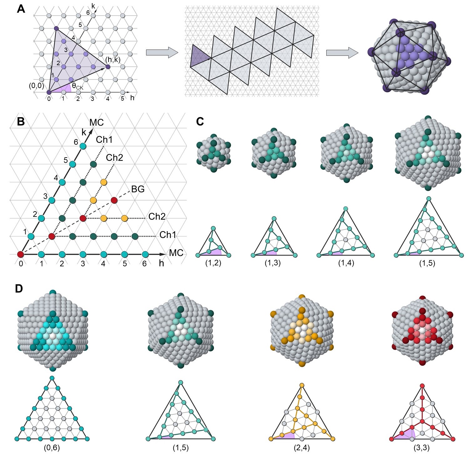
Figure 1: Caspar-Klug shells and chirality classes. A Caspar-Klug construction.[15, 35, 17] The coordinate axes $h$ and $k$ ($(h,k)$ non-negative integers) are at 60^∘. From left to right: a segment from (0,0) to $(h,k)$ is drawn and an equilateral triangle is constructed on it; the triangle is repeated 20 times to form a leaflet that is cut and folded into an icosahedral shell. B Correspondence between $(h,k)$ points and icosahedral shells. The points on the coordinate axis (light blue) correspond to achiral Mackay (MC) shells,[34, 14] those on the diagonal (red) to achiral Bergman-type (BG) shells.[36, 28] All other points correspond to chiral shells. Shells are grouped into classes Ch$n$ as explained in the text (MC$\equiv$Ch0). C The first four right-handed shells of the Ch1 class. The triangles in the bottom row (identified by their $(h,k)$) show the angle $\theta=60^{\circ}-\theta_{CK}$ between the facet edge and the line connecting the vertex to a nearest neighbour point, that decreases with increasing $k$. D Achiral and right-handed shells with $h+k=6$. From left to right, MC, Ch1, Ch2 and BG shells. $\theta$ increases from 0^∘ to 30^∘ from MC to BG. In the top rows of c and d the color shades identify symmetrically equivalent particles.

The CK construction is shown in Fig. 1A. A segment is drawn between points of coordinates (0,0) and $(h,k)$ with respect to the basis vectors of the hexagonal lattice; $h$ and $k$ are integer non-negative numbers, so that the segment always connects two lattice points. The segment is the base of an equilateral triangle, which is replicated 20 times to form a leaflet, which is then cut and folded to generate an icosahedral shell with a well-defined surface lattice.

In the CK theory, the triangulation number $T$ of an icosahedral shell is defined as the square length of the triangular edge, and is calculated as $T=h^{2}+k^{2}+hk$. Edge and radius of the shell are $\sqrt{T}$ and $\sin(2\pi/5)\sqrt{T}$, respectively. Assigning one particle to each lattice point, the shell contains $10\,T+2$ particles (see section S1 of the supplementary materials).

Shells are achiral or chiral depending on the angle $\theta_{CK}$ between the $h$-axis and the segment of the CK construction. Achiral shells correspond to segments with $\theta_{CK}=0^{\circ},30^{\circ}$ and 60^∘. Segments on a coordinate axis correspond to the achiral shells described by Mackay (MC) in his work on the packing of equal spheres [34]. Shells built on segments on the diagonal ($h=k$, $\theta_{CK}=30^{\circ}$) are here called of Bergman (BG) type, since the smallest is the outer shell of the Bergman cluster [36, 28]. All other shells are chiral, with enantiomers symmetrically placed with respect to the diagonal. We remark that, in the CK theory, an icosahedral shell is uniquely determined by the segment endpoint $(h,k)$ in the hexagonal lattice; therefore, in the following, icosahedral shells will be denoted by their $(h,k)$.

We begin our generalised construction by grouping icosahedral shells into chirality classes. In Fig. 1B, points in the hexagonal lattice are coloured according to the chirality class of the corresponding icosahedral shell. From each lattice point on the diagonal a chirality class originates, which we call Ch$n$; this comprises the $(n,n)$ BG shell, the shells with $h=n$ and $k>n$, and their enantiomers $(h>n,k=n)$. For example, shells of the Ch1 class have either $h=1$ or $k=1$, whereas the second index increases starting from 1. MC shells are grouped into class Ch$0$, together with the one-particle shell $(0,0)$. The radius and the number of particles in the shell increase with the non-constant index, so that larger and larger shells are found while moving farther from the diagonal. Shells within the same chirality class share a similar particle arrangement on the icosahedral surface, whereas shells belonging to different classes are clearly different (see Fig. 1, C and D). The grouping of icosahedral shells into chirality classes is key to rationalize and predict their optimal packing, and their dynamic assembling into tightly packed structures. This will be clarified and deeply discussed in the following.

The main point of our construction consists in assembling concentric shells into aggregates by drawing paths in the hexagonal lattice. As a first example, we consider a path along a coordinate axis, e.g., the $k$ axis (Fig. 2A), starting from $k=0$ and making steps $(0,k)\to(0,k+1)$ up to $k=i-1$. This path assembles $i$ concentric MC shells of larger and larger size into a Mackay icosahedron [34, 13], a well-known structure observed in many experiments on clusters [18, 37, 38, 19, 22], which is thus recovered as a special case of our construction. Mackay icosahedra are tightly packed structures consisting of 20 distorted tetrahedra [13] in which the particles are arranged according to the face-centered-cubic (fcc) lattice. The numbers of particles in a MC icosahedron made of $i$ shells is $N_{i}=(10i^{3}-15i^{2}+11i-3)/3$, which gives the series of magic numbers 1, 13, 55, 147, 309,…

In general, paths can be drawn by allowing different increments at each step. Here we deal with the simplest generalization, which consists of choosing between $(h,k)\to(h,k+1)$ and $(h,k)\to(h+1,k)$. In this case, the number of shells in a path from the origin to a point $(h,k)$ is $i=h+k+1$. Such paths are inspired by the Mackay path of Fig. 2A, in which one index is incremented at steps of one, whereas the other is kept constant and equal to zero. Allowing for different elementary steps in the hexagonal plane allows to build a wide variety of icosahedral structures, which retain the densely-packed character of the Mackay icosahedron.

We distinguish three cases, as shown in Fig. 2B. If $(h,k)$ is above the diagonal, the elementary move $(h,k)\to(h,k+1)$ conserves the chirality class of the shell, i.e. the shell we are adding belongs to the same class of the previous one. On the contrary, by the move $(h,k)\to(h+1,k)$ the chirality class is incremented. If $(h,k)$ is below the diagonal, the opposite applies. For $(h,k)$ in the diagonal, i.e. for shells of BG type, both steps conserve the class; specifically, the two steps are equivalent since the corresponding added shells are enantiomers, with the same size and particle arrangement but opposite chirality.

When assembling shells in physical systems, one must bear in mind that in the icosahedron the radius is shorter than the edge by $\sin(2\pi/5)\simeq 0.9511$, which has a direct effect on the packing of concentric shells. In the Mackay icosahedron of equal spheres [34], the distance between spheres in neighbouring shells is shorter by about $5\%$ than that between spheres in the same shell. Similar considerations hold for shells belonging to other chirality classes, assembled according to the path rules identified so far; in some cases, the difference between intra-shell and inter-shell nearest-neighbour distances is even larger. These considerations naturally lead to the idea of assembling shells in which particles in different shells have different sizes, which we better clarify below.

We consider the case of a core with $i$ shells, to which we add the outer shell $i+1$. Particles in the core and in the outer shell have different sizes. We define the size mismatch $sm_{i,i+1}=(d_{i+1}-d_{i})/d_{i}$, with $d_{i+1}$ and $d_{i}$ particle sizes in shells $i+1$ and $i$, respectively.

In the example of Fig. 2, C and D, the core is made of five MC shells, i.e. it is terminated by the (0,4) shell. According to our path rules, the outer shell can be either the (0,5) MC shell (same class) or the (1,4) Ch1 shell (different class). We consider a simple model, in which all particles interact by the well-known Lennard-Jones (LJ) potential; specifically, the interaction energy is the same for all particles, the only difference being the equilibrium distance of pair interactions, which accounts for particles of different sizes (see the Methods section in the supplementary materials). In Fig. 2C, we calculate the binding energy depending on the size-mismatch, and determine the mismatch that minimizes the energy of the whole aggregate. For both MC and Ch1 shells this optimal mismatch is positive, i.e. it is favourable to have bigger particles in the outer shell than in the core, and it is larger for Ch1 than for MC shells. The optimal mismatch can be estimated also by geometric packing arguments (see section S1.4 in the supplementary materials) as

$$sm_{i,i+1}=\frac{2\sin(2\pi/5)(1+\xi)\sqrt{T_{i}}+1}{2\sin(2\pi/5)\sqrt{T_{i+1}}-1}-1,$$ (1)

where $T_{i}$ and $T_{i+1}$ are triangulation numbers of shell $i$ and $i+1$, and $\xi\ll 1$ is an expansion coefficient of pair distances in the core, which depends on the number and the type of shells of the same component in the core. In Fig. 2, E and F the results of Eq. 1 are compared to those for LJ and Morse clusters. Data in Fig. 2E are obtained as in Fig. 2C, but for different sizes of the Mackay core, whereas in Fig. 2F we consider a cluster made of a Mackay core plus a Ch1 shell, to which we add a further shell of either Ch1 or Ch2 type. In all cases the agreement is good. Eq. 1 is thus a reliable guide for the semi-quantitative evaluation of the optimal mismatch, which demonstrates the key role of geometric factors in determining it.

For the path of Fig. 2, the optimal mismatch is always positive, i.e. icosahedral aggregates benefit from having bigger particles in the outer shells; in addition, much larger mismatches are found for class-changing than for class-conserving steps. These features are general for all icosahedra constructed according to the path rules identified so far, and are key to design stable icosahedral aggregates and to predict their natural growth modes.

Design strategy for icosahedral aggregates

Here we develop a path-based design strategy for icosahedral aggregates. First, a path is drawn according to the rules in Fig. 2 and, for each step, the optimal mismatch is estimated by Eq. 1. Then, particles of the appropriate sizes are associated with each shell.

An example is shown in Fig. 3, where the path connecting BG shells through neighbouring chiral shells is considered (Fig. 3A). This path alternates class-conserving and class-changing steps, spontaneously breaking mirror symmetries after the first BG shell. It produces a new series of magic numbers

$$N_{i}=\frac{1}{4}(10\,i^{3}-15\,i^{2}+18\,i-b),$$ (2)

with $b=4$ and $b=9$ for even and odd $i$, i.e. $N_{i}=1,13,45,117,239,431..$ (see section S1.2.1 of the supplementary material).

The path of Fig. 3A is used to design multi-species alkali clusters. The values of size mismatch between alkali atoms, estimated from nearest-neighbour distances in bulk crystals, are in the range of the optimal values for this path (Fig. 3B). In addition, these species present a weak tendency to mix and the bigger atoms have a smaller cohesive energy; this produces a general tendency for the bigger atoms to stay in the surface layers, which, as we have seen in the previous Section, is exactly what is needed for stabilizing icosahedral aggregates.

The clusters in Fig. 3C correspond to $i=3$ (Na₁₃@K₃₂, Na${}_{13}@$Rb₃₂) and to $i=4$ (Na${}_{13}@$K${}_{32}@$K₇₂, Na${}_{13}@$Rb${}_{32}@$Rb₇₂, Na${}_{13}@$K${}_{32}@$Rb₇₂). In these clusters, the atomic species is always changed in class-changing steps, where a large mismatch is required, while it is changed or not in class-conserving steps, where the optimal mismatch is moderate, and therefore zero mismatch is expected to be acceptable. The stability of these clusters is verified by Density Functional Theory (DFT) calculations (data are reported in tables S1-S3), specifically by checking that exchanges of pairs of different atoms in adjacent shells produce energy increases. In contrast, if MC shells of these species are assembled in the same order, the resulting clusters are energetically unstable with respect to exchanges of atomic pairs, because the mismatch between species is too large for MC shells.

Natural growth sequences

We have demonstrated how to geometrically construct multi-shell icosahedra and verified their energetic stability in various systems. Another important point is to understand how they grow dynamically in physical processes. To this end, we have performed molecular dynamics (MD) growth simulations [39], in which atoms are deposited on pre-formed clusters. This type of simulations has been used to interpret previous nanoparticle growth experiments [22, 39]. The results are shown in Fig. 3, D-H and in figs. S7-S11.

When depositing Rb atoms on a Na${}_{13}@$Rb₃₂ cluster (Fig. 3D), consisting of shells (0,0), (0,1) and (1,1), the growth begins with a spontaneous symmetry breaking to form the first chiral shell of class Ch1, i.e. shell (1,2) (or (2,1)), corresponding to the Na${}_{13}@$Rb${}_{32}@$Rb₇₂ cluster. Rb atoms self-organise to grow a chiral shell on an achiral core. This symmetry breaking is specific to BG shells, and is well predicted by the path rules. In contrast, growth on MC shells continues without symmetry breaking if atoms of the same species are deposited [22]. As Rb atoms continue to be deposited, more Ch1 shells grow. To change class after the shell (1,2), it is necessary to deposit atoms larger than Rb. From Fig. 3B, it appears that Cs atoms have the right size and in fact, depositing Cs atoms on Na${}_{13}@$Rb${}_{32}@$Rb₇₂ (Fig. 3E) results in a transition to the Ch2 class, as shells (2,2) and (2,3) form spontaneously.

Further confirmation of path rule predictivity is provided in Fig. 3, F and H. In Fig. 3F, the size mismatch for the pairs AuNi, AuCo, AuFe, AgNi, AgCo, AgCu is compared with the optimal estimates obtained from Eq. 1 for the addition of one MC and one Ch1 shell on a MC core. The mismatch much better corresponds to Ch1 than to MC shells. For AuCo, AuFe, AuNi, AgNi and AgCo, Ch1 shells should grow on MC cores of 147 or 309 atoms ($k=3$ or 4), while for AgCu the core should be larger, of 561 atoms ($k=5$). This is confirmed by MD simulations (Fig. 3, F and G) in which growth proceeds spontaneously along the Ch1 class for Ag deposited on Ni₁₄₇ or Cu₅₆₁ Mackay cores. More results are in Section S3 of the supplementary material.

In summary, the growth on top of icosahedral seeds naturally proceeds according to our rules for drawing paths in the hexagonal plane. At each stage of the growth, two possible steps (class-changing or class-conserving step) are possible; among them, the system spontaneously take the step that better fits the size mismatch between atoms of the pre-existing shell and those the growing one. If atoms of the same species are deposited, i.e. with zero mismatch, the step associated to the lower optimal mismatch is taken, which is always the class-conserving one. If one continues to deposit atoms of the same type, further and further shells belonging to the same chirality class are formed. On the other hand, the class-changing step always requires the deposition of atoms of a different species, with larger radius and with size mismatch close enough to the optimal one.

We note that almost perfect shell-by-shell growth is achieved in all simulations due to the fast diffusion of deposited atoms on top of the close-packed shells [22].

Extension to anti-Mackay shells and outlook

The mapping of icosahedral structures into paths can be extended to other cases. Here we establish the extension to the generalized anti-Mackay (AM) icosahedral shells of Fig. 4, A-C. AM shells are achiral and not close-packed, since they contain non-vertex particles with coordination lower than six. Each AM shell is identified by a couple of non-negative integers, which here we call $(p,q)$, determining the disposition of particles in the triangular facet of the shell (see Fig. 4A). Shells with $q=0$ have been described in the original work of Mackay [34], who proposed the possibility of adding to the fcc tetrahedra of the Mackay icosahedron one more shell in hexagonal close-packed (hcp) stacking. Multi-shell icosahedra terminated by AM shells of different types have been observed in confined aggregates of colloidal particles [23, 40, 25].

In Section S1.5 of the supplementary material, we demonstrate that there is a one-to-one correspondence between AM and CK shells, as an AM shell of indexes $(p,q)$ has the same number of particles of the CK shells with $h=q+1$, $k=p+q$, if $k>h$, or $k=q+1$, $h=p+q$ if $h>k$ ($p=1$ gives the BG shells, that are common to AM and CK structures). Therefore we can unambiguously identify an AM shell by the $(h,k)$ indexes of the corresponding CK shell, and assign to it the same lattice point on the hexagonal plane. We group AM shells into AM$n$ classes and denote an AM shell by $(h,k)^{*}$. The correspondence between AM$n$ and Ch$n$ shells is explicitly shown in Fig. 4B,C for $n=1,2$.

AM shells can be packed by using the same rules described for CK ones. The same elementary steps in the hexagonal plane are allowed, but now one can decide whether to consider the CK or the AM version corresponding to the endpoint of the step. In this way a larger variety of icosahedra can be built. Again, the stability of these structures is provided by the size mismatch between particles in different shells. The optimal size mismatch for icosahedra with AM shells can be estimated by using the same geometric considerations made for CK shells (see Section S1.5 of the supplementary material). In Fig. 4D we compare the stability of all possible shells that can be put on top of a Mackay core, namely MC, Ch1 and AM1. The optimal mismatch of the AM1 shells is intermediate between those of the MC and Ch1 shells (see also fig. S3). The mismatch for adding a AM1 shell on a 147-atom Mackay core is close to the one of AgCu, so that AM shells should grow by depositing Ag atoms on Cu a Mackay core of this size. This is verified by the MD simulations of Fig. 4E, in which we observe the formation of an Ag $(1,3)^{\ast}$ shell. The growth proceeds quite differently from that of Fig. 3H: a second shell of AM2 type is formed, followed by a shell of BG type, i.e. the class is changed at each step. This behaviour is due to the fourfold adsorption sites on the surface of AM shells, which act as adatom traps and naturally leads to the formation of AM shells of higher class (see fig. S12 for details on the growth mechanism). We note that traps make the growing structure much less smooth than in the case of Fig. 3H.

Our construction can be further generalized. Let us mention a few possibilities. First, the paths can begin at any point in the lattice, instead of (0,0), so that the shells enclose an empty volume. Multi-shell structures enclosing a cavity are relevant to biological systems [41, 42, 32], and have been observed in metal clusters [43]. Second, the non-equivalent sites of a shell can be decorated with different types of particles, while maintaining icosahedral symmetry. For example, the vertex atoms in the surface shell of a metal cluster can be of a different species than the other atoms, thus becoming isolated impurities embedded in a surface of a different material. This possibility is relevant to single-atom catalysis [44]. Moreover, the mapping into paths may be applied to other figures obtained by cutting and folding the hexagonal lattice, such as octahedra and tetrahedra, and to other lattices, including Archimedean lattices [17], that can better accommodate particles with non-spherically symmetric interactions. In summary, the mapping into paths is a powerful tool for the bottom-up design of chiral and achiral aggregates of atoms, colloids and complex molecules. The unusual geometries of these aggregates can be of interest in various fields, e.g. in catalysis, optics and synthetic biology.

Supplementary materials

Methods
Supplementary Text
Figs. S1 to S12
Tables S1 to S3
References (46-53)

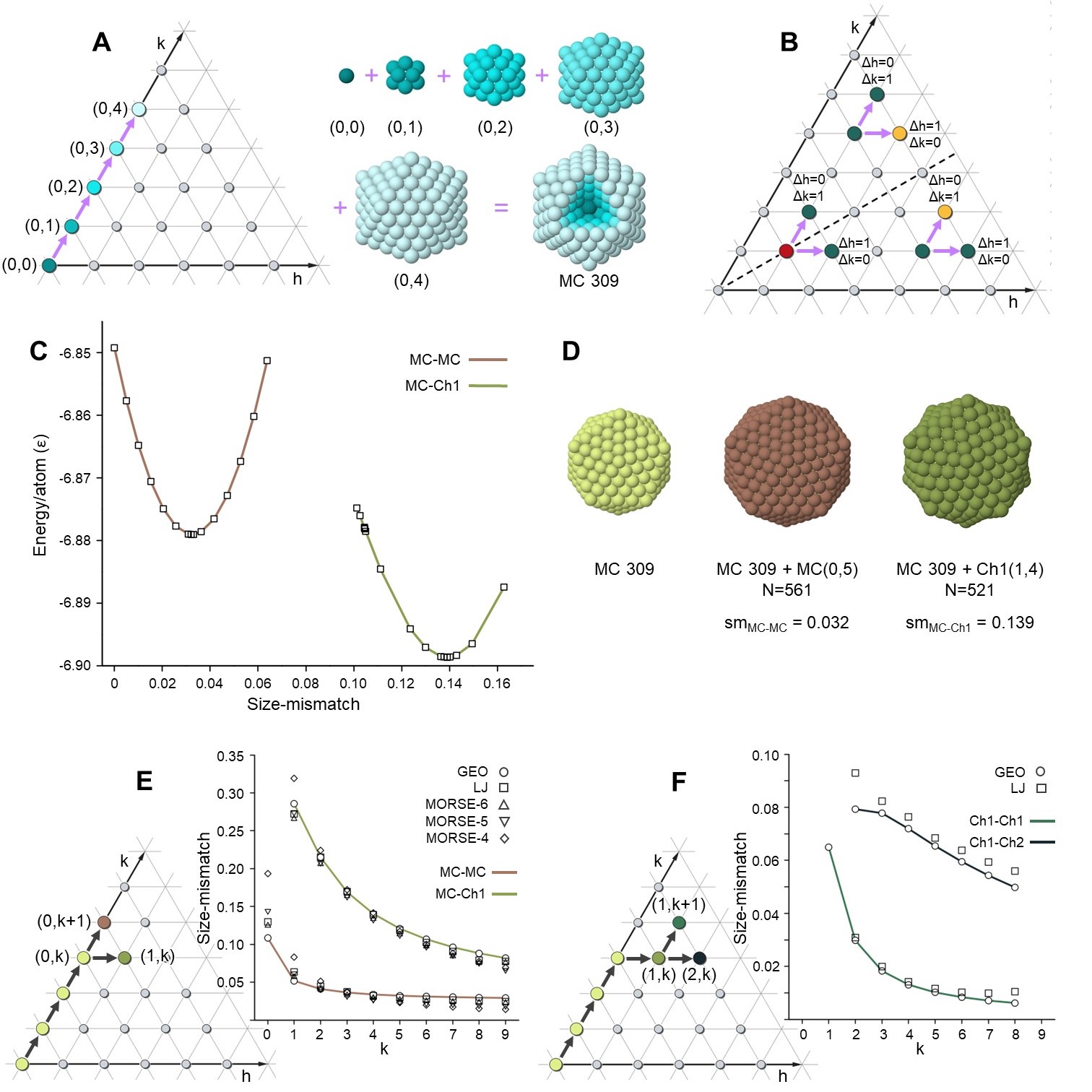
Figure 2: Mapping icosahedra into paths. A Path of a Mackay icosahedron: $i=5$ shells are assembled on top of each other. B The three possible cases when choosing between $(h,k)\to(h,k+1)$ and $(h,k)\to(h+1,k)$ at each step of the path. C Binding energy per atom for clusters made of a core with five MC shells plus a sixth shell, which is either MC or Ch1. Interactions are of Lennard-Jones (LJ) type (see Methods Section in the supplementary material). The particles of the sixth shell differ from those in the core only by their size. The energy is in units of the $\varepsilon$ of the LJ potential. The structures are shown in D. E Comparison of the optimal mismatch between steps $(0,k)\to(0,k+1)$ and $(0,k)\to(1,k)$, corresponding to additional MC and Ch1 shells on an MC core, respectively. The optimal mismatch of Eq. 1 (GEO values) is compared to Lennard-Jones (LJ) and Morse potential results. The Morse potential data are given for three values (4,5,6) of the parameter $\alpha$, that regulates the width of the potential well (see Methods Section in the supplementary material). F Comparison between steps $(1,k)\to(1,k+1)$ and $(1,k)\to(2,k)$, corresponding to additional Ch1 and Ch2 shells on a core containing $k$ MC and one Ch1 shells, respectively. The optimal mismatch of Eq. 1 (GEO) is compared to LJ data.

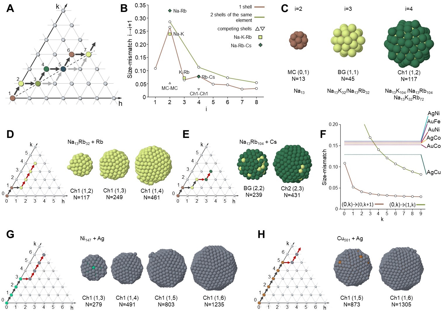
Figure 3: Chiral cluster structures and growth sequences. A A path connecting all BG shells through their nearby chiral shells. Black and grey arrows indicate paths with right and left-handed chiral shells. A generic path of this type may alternate both chiralities, corresponding to combinations of black and grey arrows. Shells are enumerated along the black-arrow path. B Optimal mismatch $sm_{i,i+1}$ according to Eq. 1 for the path in A. Points connected by brown and green lines correspond to changes of species every shell and every two shells. The optimal $sm_{i,i+1}$ are compared to the mismatch between pairs of atomic species, indicated by squares and diamonds. The triangles correspond to the optimal mismatch between two MC shells and two Ch1 shells. C Structures for $i=2,3,4$ along the path of A, with their compositions related to specific systems. D-E Growth sequences from MD simulations for alkali metal clusters and corresponding paths. D Rb atoms are deposited on an icosahedral Na${}_{13}@$Rb₃₂ seed, E the seed is Na${}_{13}@$Rb₁₀₄ on which Cs atoms are deposited. F Size mismatch for some transition metal pairs compared to the optimal mismatch for a MC and a Ch1 shell on a MC core (green and brown lines, respectively), as a function of core size. G-H Snapshots from growth simulations and corresponding paths for the deposition of Ag atoms on G Ni₁₄₇ and H Cu₅₆₁ cores. All simulation snapshots in D-E, G-H are taken at magic sizes for the corresponding paths.

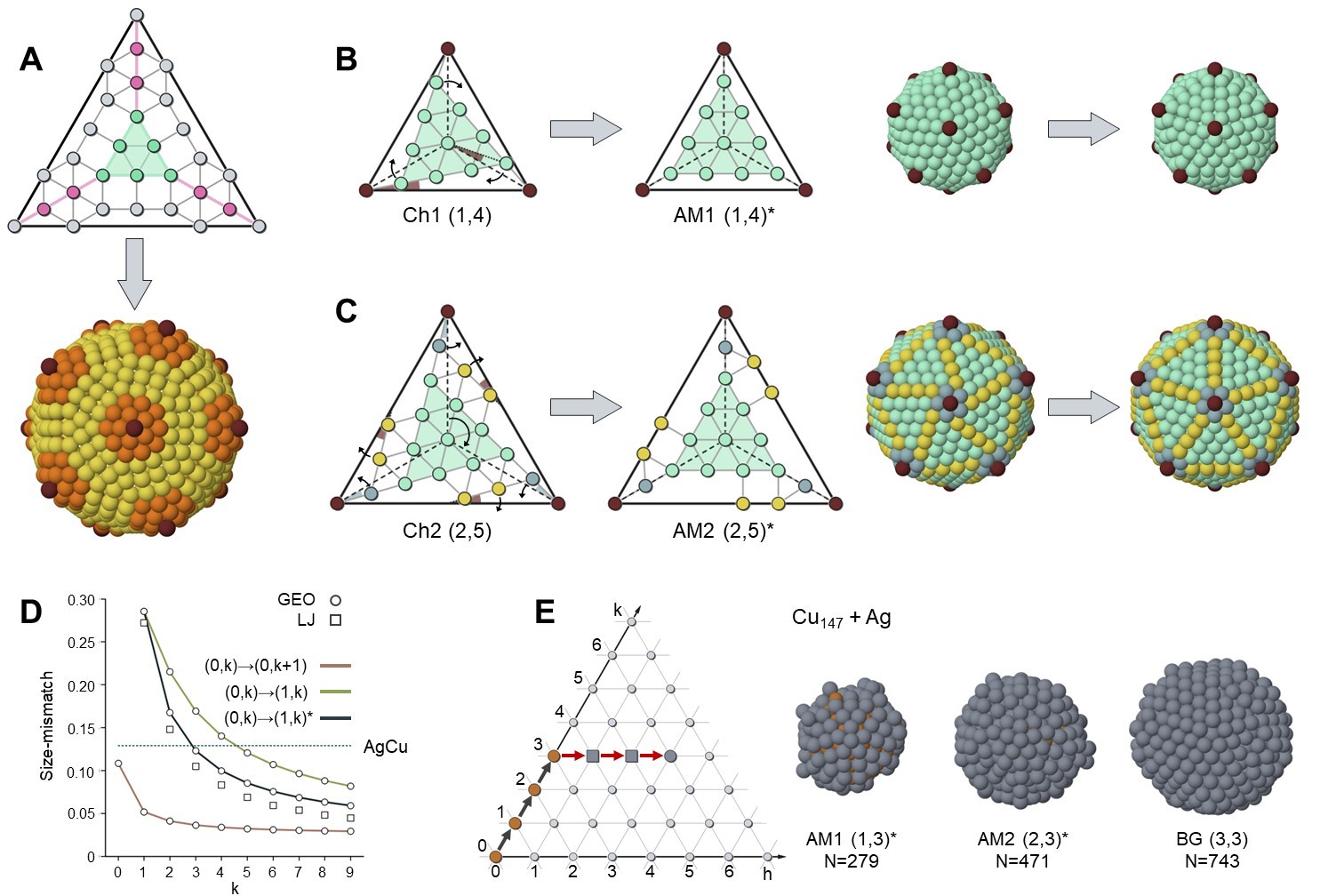
Figure 4: Generalized anti-Mackay shells and their growth paths. A A shell of the AM family. A facet and the complete shell are shown in the upper and lower panels. The shell is identified by $(p,q)$, with $p$ number of particles on the side of the inner triangle (light green particles in the top panel) and $q$ number of particles between nearby vertices of the outer and inner triangles (pink particles). In this case, $(p,q)=(3,2)$. In the bottom panel, orange particles have coordination 6 within the shell, while other particles have lower coordination. B AM1$\leftrightarrow$Ch1 and C AM2$\leftrightarrow$Ch2 correspondences. AM1$\leftrightarrow$Ch1 amounts to the rotation of the inner triangles [45], whereas AM2$\leftrightarrow$Ch2 involves rotations of different groups of particles, represented by different colours. A more detailed description is in Supplementary Discussion SD-1. D Optimal mismatch for one AM1 shell on a Mackay core ($(0,k)\to(1,k)^{*}$) as a function of core size, compared with Ch1 ($(0,k)\to(1,k)$) and Mackay shells ($(0,k)\to(0,k+1)$), for Lennard-Jones clusters. GEO values are calculated by the formula derived in Section S1.5 of the supplementary material. The mismatch between Ag and Cu is indicated. E Snapshots from a MD growth simulation in which Ag atoms are deposited on a Mackay Cu₁₄₇ core and corresponding path, with AM shells indicated by squares.

Supplementary Material for
Path-based packing of icosahedral shells into multi-component aggregates
Nicolò Canestrari, Diana Nelli,^∗ Riccardo Ferrando^∗
Dipartimento di Fisica, Università di Genova, Via Dodecaneso 33, 16146 Genova, Italy

^∗To whom correspondence should be addressed;

E-mail: diana.nelli@edu.unige.it; riccardo.ferrando@unige.it.

Methods

Construction of the structures. Icosahedral structures are built by assembling Caspar-Klug and anti-Mackay shells by a purposely written C++ code. The code takes as input the geometric features of each shell, i.e. the indexes $h$ and $k$ of the CK construction, the distance $d$ between particles, and the shell type (either CK or AM). For CK shells, the first 12 particles are placed in the vertices of the icosahedron of edge legth $\sin(2\pi/5)\sqrt{T}\,d$. The other particles are placed on the icosahedral facets according to the CK scheme: on each facet plane a 2D hexagonal lattice is built, which is rotated of an angle of amplitude $\theta_{CK}$ with respect to one of the facet edges; particles are placed on lattice points falling within the facet. For AM shells, the indexes $p$ and $q$ are calculated as $p=k-h+1$, $q=h-1$ if $k\geq h$, $p=h-k+1$, $q=k-1$ otherwise. The first 12 particles are placed in the vertices of the icosahedron of edge length $(p+\sqrt{3}\,q+\sqrt{3}-1)\,d$. The other particles are placed on the icosahedral facets according to scheme of Fig. 4A in the main text. A more detailed description of CK and AM shells and of the procedure for constructing them can be found in Section S1 of the Supplementary Text.

Lennard-Jones (LJ) and Morse potential calculations. Both potentials are pair potentials, in which the total energy $E$ is written as

$$E=\frac{1}{2}\sum_{i\neq j}u(r_{ij}),$$ (3)

where $r_{ij}=|\mathbf{r_{j}}-\mathbf{r_{j}}|$ is the distance between a pair of particles. The LJ potential is written as

$$u(r)=\varepsilon\left[\left(\frac{r_{m}}{r}\right)^{12}-2\left(\frac{r_{m}}{r}\right)^{6}\right],$$ (4)

where $\varepsilon$ is the well depth and $r_{m}$ is the equilibrium distance, which corresponds to the particle size $d$. The Morse potential is written as

$$u(r)=\varepsilon\left[\mathrm{e}^{-2\alpha(r/r_{m}-1)}-2\mathrm{e}^{-\alpha(r/r_{m}-1)}\right],$$ (5)

where the dimensionless parameter $\alpha$ regulates the width of the potential well, that decreases with increasing $\alpha$. For $\alpha=6$ both LJ and Morse potential have the same width of the well, i.e. the same curvature at the well bottom. In the simulations of Fig. 2, C, E and F in the main text all particles were given the same value of $\varepsilon$ (and of $\alpha$ for the Morse potential), but particles of the outer shell and of the core were given different sizes (i.e. $r_{m}=r_{m,c}$ for core particles and $r_{m}=r_{m,s}$ for outer shell particles). For interactions between particles of the core and the outer shell $r_{m,cs}=(r_{m,c}+r_{m,s})/2$. The structures were locally relaxed by quenched molecular dynamics [46] to reach the position of the local minimum in the energy landscape.

Density Functional Theory (DFT) calculations. All DFT calculations were made by the open-source QUANTUM ESPRESSO software [47] using the Perdew-Burke-Ernzerhof exchange-correlation functional [48]. The convergence thresholds for the total energy, total force, and for electronic calculations were set to 10^-4 Ry, 10^-3 Ry/a.u. and 5 $\times$ 10^-6 Ry espectively. We used a periodic cubic cell, whose size was set to 26-48 Å, depending on the size of the cluster, in order to ensure at least a 10 Å  separation between clusters in different periodic images. Cutoffs for wavefunction and charge density were set to 66 and 323 Ry, according to Na.pbe-spn-kjpaw_psl.1.0.0.UPF, K.pbe-spn-kjpaw_psl.1.0.0.UPF, Rb.pbe-spn-kjpaw_psl.1.0.0.UPF as provided by the QUANTUM ESPRESSO pseudopotential library available at
http://pseudopotentials.quantum-espresso.org/legacy\_tables/ps-library/.

Molecular dynamics (MD) growth simulations. Molecular Dynamics (MD) growth simulations are made by molecular dynamics using the same type of procedure adopted in Ref. [39, 22]. The equations of motion are solved by the Velocity Verlet algorithm with a time step of 5 fs for the simulations of AgNi, AgCu, AgCo, AuCo, AuFe, AgPdNi and 2 fs for the simulations of NaK, NaRb, NaKRb, NaRbCs. In all simulations, the temperature is kept constant by an Andersen thermostat with a collision frequency of 5 10¹¹ s^-1. Simulations start from a seed, which is an initial cluster, then atoms are deposited one by one on top of it in an isotropic way from random directions at a constant rate. The simulation of Fig. 3D in the main text was started from a Na${}_{13}@$K₃₂ Bergman-type seed corresponding to the path arriving to $(h,k)=(1,1)$ and Rb atoms were deposited at a rate of 0.1 atoms/ns and at a temperature of 125 K. The simulation of Fig. 3E in the main text was started from a Na${}_{13}@$Rb${}_{32}@$Rb₇₂ chiral seed corresponding to the path arriving to $(h,k)=(1,2)$ and Cs atoms were deposited at a rate of 0.1 atoms/ns at 125 K. The simulation of Fig. 3G in the main text was started from a Ni₁₄₇ Mackay icosahedral seed corresponding to the path arriving to $(h,k)=(0,3)$ and Ag atoms were deposited at a rate of 0.1 atoms/ns at 450 K. The simulation of Fig. 3H in the main text was started from a Cu₅₆₁ Mackay icosahedral seed corresponding to the path arriving to $(h,k)=(0,5)$ and Ag atoms were deposited at a rate of 0.1 atoms/ns at 450 K. The simulation of Fig. 4E in the main text was started from a Cu₁₄₇ Mackay icosahedral seed corresponding to the path arriving to $(h,k)=(0,3)$ and Ag atoms were deposited at a rate of 1 atoms/ns at 350 K. For all systems, atom-atom interactions were modelled by an atomistic force field, which is known as Gupta potential [49]. Form and parameters of the potential can be found in Refs. [50, 51, 52, 53].

Supplementary Text

Appendix S1 Construction of the structures and optimal mismatch

S1.1 Number of particles in a CK shell

The number of particle in a Caspar-Klug (CK) shell can be calculated from the ratio between the area of the triangular facet of the icosahedron and the area occupied by a particle on the CK plane. Icosahedral facets are equilateral triangles of side length $\sqrt{T}$, $T$ being the triangulation number of the CK shell. Therefore the area of the facet is

$$A_{T}=\frac{1}{2}\sqrt{T}\sqrt{T}\sin{60^{\circ}}=\frac{1}{2}T\frac{\sqrt{3}}{2}=\frac{\sqrt{3}}{4}T.$$ (S1)

The area occupied by a particle corresponds to the area of the unit cell of the 2D hexagonal lattice with unit distance between two nearby lattice points, which is

$$A_{P}=\frac{\sqrt{3}}{2}.$$ (S2)

Therefore the number of particles in a triangular facet of the CK icosahedron is

$$N_{T}=\frac{A_{T}}{A_{P}}=\frac{\frac{\sqrt{3}}{4}T}{\frac{\sqrt{3}}{2}}=\frac{T}{2}.$$ (S3)

To calculate the total number of particles in the shell we multiply $N_{T}$ by the number of facets in the icosahedron, which is 20. However, we need to be careful when considering icosahedral vertices. In the calculation of $N_{T}$, the number of particles assigned to each vertex is 1/6, since it is shared among 6 equilateral triangles in the hexagonal lattice, while in the icosahedron, each vertex is shared among 5 facets. As a consequence, if we calculate the total number of particles as $20N_{T}$, we are assigning to each vertex 5/6 particles instead of 1. Therefore we need to add further 1/6 particles per vertex. Since the icosahedron has 12 vertices, 2 particles have to be added. The number of particles in the CK icosahedral shell is therefore

$$N_{SHELL}=20\,N_{T}+2=10\,T+2.$$ (S4)

S1.2 Magic numbers

Eq. S4 can be used to calculate the magic numbers of any icosahedral series, i.e. of icosahedra mapped into any pathway in the closed-packed plane. We recall that magic numbers are those sizes at which perfect icosahedra can be built, and therefore correspond to the completion of the different concentric CK shells. Here we calculate the magic numbers of two interesting icosahedral series, i.e.

1. the series in Fig. 3A in the main text, passing through shells of Bergman (BG) type each two steps; here we call it BG icosahedral series;

2. the series of core-shell icosahedra with a Mackay (MC) core surrounded by a thick layer of shells of chiral-1 (Ch1) type, as are obtained in the growth of Ni@Ag and Cu@Ag core@shell nanoparticles (see Figs. 3, G and H in the main text).

S1.2.1 The BG series

The pathway in the closed-packed plane corresponding to the BG icosahedral series is

$$(0,0)\rightarrow(0,1)\rightarrow(1,1)\rightarrow(1,2)\rightarrow(2,2)\rightarrow(2,3)\rightarrow...\rightarrow(h,h)\rightarrow(h,h+1)\rightarrow...$$ (S5)

The index $h$ is incremented by 1 every two steps, from 0 to $h_{max}$; the first and the second shell of index $h$ have $k=h$ and $k=h+1$, respectively. We consider an icosahedron made of $i$ shells. If $i$ is even, the maximum value of $h$ is

$$h_{max}=\frac{i-2}{2},$$ (S6)

and, in the last shell, $k=h_{max}+1$. On the other hand, if $i$ is odd, we have

$$h_{max}=\frac{i-1}{2},$$ (S7)

and, in the last shell, $k=h_{max}$. We calculate the total number of particles in the icosahedron, in both cases. For even $i$, we have

$$\begin{split}N_{EVEN}&=\sum_{h=0}^{h_{max}}\sum_{k=h}^{h+1}(10\,T^{(h,k)}+2)-1=\\ &=\sum_{h=0}^{h_{max}}\sum_{k=h}^{h+1}\left[10\,(h^{2}+k^{2}+hk)+2\right]-1.\end{split}$$ (S8)

Here we sum up the number of particles in each CK shell, up to $(h_{max},h_{max}+1)$. The sizes of the shells are given by Eq. S4, except for the first shell, namely $(0,0)$; if we calculate the size of such shell by Eq. S4 we would obtain 2, which is wrong since the shell is made of only one particles. Therefore, if we use Eq. S4 for all shells, we have to subtract 1 particle from the final result. By writing explicitly the two terms $k=h$ and $k=h+1$, we obtain

$$\begin{split}N_{EVEN}&=\sum_{h=0}^{h_{max}}(60\,h^{2}+30\,h+14)-1=\\ &=60\sum_{h=0}^{h_{max}}h^{2}+30\sum_{h=0}^{h_{max}}h+14\sum_{h=0}^{h_{max}}1-1.\end{split}$$ (S9)

By using the equivalences

$$\begin{split}\sum_{h=0}^{h_{max}}h&=\frac{h_{max}(h_{max}+1)}{2},\\ \sum_{h=0}^{h_{max}}h^{2}&=\frac{h_{max}(h_{max}+1)(2h_{max}+1)}{6},\end{split}$$ (S10)

we calculate

$$N_{EVEN}=20h_{max}^{3}+45h_{max}^{2}+39h_{max}+13.$$ (S11)

Finally, we use the relation in Eq. S6 to write the total number of particles as function of the number of icosahedral shells

$$N^{(i)}_{EVEN}=\frac{5}{2}i^{3}-\frac{15}{4}i^{2}+\frac{9}{2}i-1.$$ (S12)

If $i$ is odd, the CK indexes of the last shell are $(h_{max},h_{max})$. The total number of particles in the icosahedron can be easily calculated, by subtracting from $N_{EVEN}$ the number of particles in the shell $(h_{max},h_{max}+1)$:

$$\begin{split}N_{ODD}&=N_{EVEN}-N_{SHELL}^{(h_{max},h_{max}+1)}=\\ &=20h_{max}^{3}+45h_{max}^{2}+39h_{max}+13-(30h_{max}^{2}+30h_{max}+12)=\\ &=20h_{max}^{3}+15h_{max}^{2}+9h_{max}+1.\end{split}$$ (S13)

By using the relation in Eq. S7 we obtain

$$N^{(i)}_{ODD}=\frac{5}{2}i^{3}-\frac{15}{4}i^{2}+\frac{9}{2}i-\frac{9}{4}.$$ (6)

The number of particles in a icosahedron of the BG series made of $i$ shells is therefore

$$N^{(i)}_{BG}=\frac{1}{4}(10i^{3}-15i^{2}+18i-b),$$ (S14)

with

$$b=\begin{cases}4\text{ if $i$ is even}\\ 9\text{ if $i$ is odd}\end{cases}.$$ (S15)

S1.2.2 MC@Ch1 series

We consider an icosahedron made of $i$ MC shells, surrounded by $j$ Ch1 shells. The corresponding pathway in the closed-packed plane is

$$(0,0)\rightarrow(0,1)\rightarrow...\rightarrow(0,i-1)\rightarrow(1,i-1)\rightarrow(1,i)\rightarrow...\rightarrow(1,i+j-2)$$ (7)

The number of particles in the icosahedron is given by the sum of the number of particles in the MC core and the number of particles in the Ch1 shells. In the core, we have

$$\begin{split}N_{MC}^{(i)}&=\sum_{k=0}^{i-1}(10\,T^{(0,k)}+2)-1=\\ &=\sum_{k=0}^{i-1}(10k^{2}+2)-1=\\ &=\frac{10}{3}i^{3}-5i^{2}+\frac{11}{3}i-1\end{split}$$ (S16)

particles, which is the well-known formula for MC icosahedral magic numbers. The total number of particles in the Ch1 shells is

$$\begin{split}N_{Ch1}^{(i,j)}&=\sum_{k=i-1}^{i+j-2}(10\,T^{(1,k)}+2)=\\ &=\sum_{k=i-1}^{i+j-2}\left[10(k^{2}+k+1)+2\right]=\\ &=\sum_{k=i-1}^{i+j-2}(10k^{2}+10k+12).\end{split}$$ (S17)

In order to use the equivalences of Eq. S10, we introduce the index $l=k-i+1$ . We can write

$$\begin{split}N_{Ch1}^{(i,j)}&=\sum_{l=0}^{j-1}\left[10(l+i-1)^{2}+10(l+i-1)+12\right]=\\ &=\sum_{l=0}^{j-1}\left[10l^{2}+(20i-10)l+10i^{2}-10i+12\right],\end{split}$$ (S18)

and finally we calculate

$$N_{Ch1}^{(i,j)}=j\left(10i^{2}+\frac{10}{3}j^{2}+10ij-20i-10j+\frac{56}{3}\right).$$ (S19)

The total number of particles in the MC@Ch1 icosahedron is therefore

$$N_{MC@Ch1}^{(i,j)}=N_{MC}^{(i)}+N_{Ch1}^{(i,j)}.$$ (S20)

We can obtain different series of magic numbers by fixing the size of the MC core and adding Ch1 shells one after the other on top of it. Here we report the first magic numbers for some series of this kind.

• 2 MC shells: 1, 13, 45, 117, 249, 461, 773, 1205, …

• 3 MC shells: 1, 13, 55, 127, 259, 471, 783, 1215, …

• 4 MC shells: 1, 13, 55, 147, 279, 491, 803, 1235, …

• 5 MC shells: 1, 13, 55, 147, 309, 521, 833, 1265, …

• 6 MC shells: 1, 13, 55, 147, 309, 561, 873, 1305, …

S1.3 Implementation of the construction of a CK shell

Here we explain in details how the construction of CK shells is implemented in our C++ code. In the CK scheme, each icosahedral facet is an equilateral triangle whose vertices are lattice points of a 2D hexagonal lattice. The coordinates of the vertices are given with respect to the the primitive vectors $\mathbf{a}_{1}$ and $\mathbf{a}_{2}$, forming an angle of $60^{\circ}$ (see Fig. SS1A): $V_{1}(0,0)$, $V_{2}(h,k)$, $V_{3}(-k,h+k)$, where the positive integers $h$ and $k$ are the indexes of the CK construction, that unambiguously determine the icosahedral shell structure. All lattice points within the triangle belong to the CK shell, i.e. a lattice point $P(i_{1},i_{2})$ belongs to the shell if $i_{1}$ and $i_{2}$ meet the following conditions:

$$\begin{cases}k\,i_{1}-h\,i_{2}\leq 0\\ (h+k)\,i_{1}+k\,i_{2}\geq 0\\ h\,i_{1}+(h+k)\,i_{2}\leq T\end{cases}$$ (S21)

where $T$ is the square distance between the vertices, i.e.

$$T=h^{2}+k^{2}+hk.$$ (S22)

It is useful to write the point $P$ with respect to the vectors $\mathbf{a}_{1}^{\prime}$ and $\mathbf{a}_{2}^{\prime}$, lying on two adjacent sides of the triangle. These are obtained by rotating the primitive vectors of the hexagonal lattice counterclockwise of an angle $\theta_{CK}$ (see Fig. S1B). The primitive vectors can be written as

$$\begin{cases}\mathbf{a}_{1}=\left(\cos{\theta_{CK}}+\dfrac{\sin{\theta_{CK}}}{\sqrt{3}}\right)\mathbf{a}_{1}^{\prime}-\dfrac{2\sin{\theta_{CK}}}{\sqrt{3}}\mathbf{a}_{2}^{\prime}\\ \mathbf{a}_{2}=\dfrac{2\sin{\theta_{CK}}}{\sqrt{3}}\mathbf{a}_{1}^{\prime}+\left(\cos{\theta_{CK}}-\dfrac{\sin{\theta_{CK}}}{\sqrt{3}}\right)\mathbf{a}_{2}^{\prime}\end{cases}$$ (S23)

The cosine and sine of $\theta_{CK}$ are calculated from the CK indexes, as

$$\cos{\theta_{CK}}=\dfrac{2h+k}{2\sqrt{T}},\\$$ (S24)

$$\sin{\theta_{CK}}=\dfrac{\sqrt{3}\,k}{2\sqrt{T}}.$$ (S25)

The coordinates of the lattice point $P$ can therefore be expressed as

$$P-V_{1}=\left\{i_{1}\cos{\theta_{CK}}+(i_{1}+2i_{2})\frac{\sin{\theta_{CK}}}{\sqrt{3}}\right\}\mathbf{a}_{1}^{\prime}+\left\{i_{2}\cos{\theta_{CK}}-(2i_{1}+i_{2})\frac{\sin{\theta_{CK}}}{\sqrt{3}}\right\}\mathbf{a_{2}}^{\prime}.$$ (S26)

For building a CK icosahedral shell by our C++ code, the CK indexes $h$ and $k$ and the inter-particle distance $d_{CK}$ have to be set by user. The quantities $T$, $\cos{\theta_{CK}}$ and $\sin{\theta_{CK}}$ are calculated, then the CK is built in according to the following scheme:

1. The first 12 particles are placed in the vertices of the icosahedron of edge length $d_{CK}\,\sqrt{T}$.

2. For each triplet of vertices $V_{1}$, $V_{2}$, $V_{3}$ forming an icosahedral facet, the vectors $\mathbf{a}_{1}^{\prime}$ and $\mathbf{a_{2}}^{\prime}$ are calculated as

   $$\mathbf{a}_{1}^{\prime}=\frac{V_{2}-V_{1}}{\sqrt{T}},\\$$ (S27)

   $$\mathbf{a}_{2}^{\prime}=\frac{V_{3}-V_{1}}{\sqrt{T}}.$$ (S28)

3. Particles within the icosahedral facet are placed on points with coordinates given by Eq. S26, for all couples of indexes $i_{1}$, $i_{2}$ meeting the conditions of Eq. S21.

S1.4 Evaluation of the optimal size mismatch in CK icosahedra

Here we discuss the evaluation of the optimal size mismatch between particles in different shells of a multi-shell CK icosahedron. We start by evaluating the optimal size mismatch in core-shell icosahedra made of a MC core surrounded by one shell of either MC or Ch1 type (namely MC@MC and MC@Ch1 icosahedra); then, we extend our results to structures made of CK shells belonging to any chirality class.

S1.4.1 Optimal size mismatch in the MC@MC icosahedron

In MC shells, one of the CK indexes is equal to zero. Here we consider icosahedral shells with $k\geq h$; therefore MC shells have $h=0$, whereas $k$ can take any integer value. The triangulation number is

$$T_{MC}^{(k)}=k^{2},$$ (8)

therefore the radius of the shell is

$$r_{MC}^{(k)}=d_{CK}\sin\left(\frac{2\pi}{5}\right)k,$$ (S29)

$d_{CK}$ being the inter-particle distance in the 2D hexagonal plane. The MC icosahedron is made of concentric MC shells. Let us now calculate inter-shell distances, i.e. distances between icosahedral vertices belonging to nearby shells. This corresponds to the difference between the radii

$$\begin{split}\Delta r&=r_{MC}^{(k+1)}-r_{MC}^{(k)}=\\ &=(k+1)\,d_{CK}\sin{\left(\frac{2\pi}{5}\right)}-k\,d_{CK}\sin{\left(\frac{2\pi}{5}\right)}=\\ &=d_{CK}\sin{\left(\frac{2\pi}{5}\right)}\approx 0.9511\,d_{CK}\end{split}$$ (S30)

The inter-shell distance is the same for all pairs of nearby shells, and it is smaller than the intra-shell distance by about 5%. It is possible to verify that all nearest-neighbours distances between particles in the same shell are equal to $d_{CK}$, and those between particles in nearby shells are equal to $\Delta r$; therefore, in the MC icosahedron, the inter-particle distance spectrum has only two peaks, in $\Delta r$ and $d_{CK}$.

Let us now consider a MC icosahedron made of identical spherical particles. We denote by $d$ the ideal pair distance of the system. In the case of metal atoms, $d$ corresponds to the ideal interatomic distance in the bulk crystal. Since intra-shell and inter-shell distances within the MC icosahedron are different, it is not possible to build a structure of this kind in which all pair distances are equal to $d$. However, we expect the icosahedron to be stable if pair distances are close enough to the ideal value. We want to quantify this concept, i.e. to determine what is the optimal MC icosahedral arrangement when packing particles of the same type. Such optimal arrangement depends on the ability of the particles (spheres, atoms, molecules, …) to adapt pair distances, by expanding or compressing them from the ideal value. Here we consider a system in which pair distances can contract and expand symmetrically around the ideal distance. This model should describe reasonably well the behaviour of atomic systems. In such a system, $\Delta r$ and $d_{CK}$ are expected to be displaced from $d$ by the same amount, i.e.

$$d_{CK}=(1+\xi)\,d,$$ (S31)

$$\Delta r=(1-\xi)\,d.$$ (S32)

By using the relation between inter- and intra-shell distances in Eq. S30, we find the optimal expansion/contraction coefficient $\xi_{MC}$ of pair distances for a MC icosahedron made of spherical particles of a single type

$$\xi_{MC}=\frac{1-\sin{\left(\frac{2\pi}{5}\right)}}{1+\sin{\left(\frac{2\pi}{5}\right)}}\approx 0.0251.$$ (S33)

Now we consider bi-elemental icosahedra of core-shell type. The icosahedron is made of two parts: an internal core, which is an icosahedron made of multiple concentric MC shells, and a single external MC shell, of a different element. Ideal pair distances in the core and in the shell are $d_{CORE}$ and $d_{SHELL}$, respectively. We denote by $k$ the index of the most external shell of the core; the index of the shell is therefore $k+1$. For the core, we consider the optimal MC icosahedral arrangement, in which intra-shell distances are expanded by $\xi_{MC}$ compared to the ideal distance $d_{CORE}$. The radius of the core is given by Eq. S29, and it is

$$r_{CORE}=k\sin{\left(\frac{2\pi}{5}\right)}(1+\xi_{MC})\,d_{CORE}.$$ (S34)

Since the shell is made of one single MC layer, all pair distances within the shell are equal; in the optimal shell, such distances are equal to the ideal value $d_{SHELL}$. The radius of the shell is therefore

$$r_{SHELL}=(k+1)\sin{\left(\frac{2\pi}{5}\right)}\,d_{SHELL}.$$ (S35)

The core-shell distance is given by

$$\begin{split}\Delta r_{CORE-SHELL}&=r_{SHELL}-r_{CORE}=\\ &=(k+1)\sin{\left(\frac{2\pi}{5}\right)}\,d_{SHELL}-k\sin{\left(\frac{2\pi}{5}\right)}(1+\xi_{MC})\,d_{CORE},\end{split}$$ (S36)

In the optimal core-shell icosahedron, the core-shell distance exactly corresponds to the ideal value

$$d_{CORE-SHELL}=\frac{d_{CORE}+d_{SHELL}}{2}.$$ (S37)

In this way, the pair distance distribution within the whole structure is as close as possible to the ideal interatomic distances $d_{CORE}$, $d_{SHELL}$ and $d_{CORE-SHELL}$. We note that $\Delta r$ corresponds to the distance between particles in nearby vertex of adjacent shells. If such shells are made of the same atom type, all inter-shell nearest-neighbour distances are equal to $\Delta r$, but this is not true for shells made of particles of different sizes, in which a more complex nearest-neighbour distance spectrum arises. The condition $\Delta r=d_{CORE-SHELL}$ is therefore to be taken as an approximate condition, which, as we will see in the following, allows to establish an approximate relationship between $d_{CORE}$ and $d_{SHELL}$.

The condition on $\Delta r$ translates into the following relation between $d_{CORE}$ and $d_{SHELL}$ :

$$(k+1)\sin{\left(\frac{2\pi}{5}\right)}\,d_{SHELL}-k\sin{\left(\frac{2\pi}{5}\right)}(1+\xi_{MC})\,d_{CORE}=\frac{d_{CORE}+d_{SHELL}}{2}.$$ (S38)

We define the ratio

$$\alpha=\frac{d_{SHELL}}{d_{CORE}}$$ (S39)

between ideal interatomic distances in the core and in the shell. Eq. S38 can be written in terms of $\alpha$, as

$$(k+1)\sin{\left(\frac{2\pi}{5}\right)}\,\alpha-k\sin{\left(\frac{2\pi}{5}\right)}(1+\xi_{MC})=\frac{1+\alpha}{2}.$$ (S40)

We can therefore find the ideal value $\alpha_{MC-MC}$ for which the optimal core-shell MC@MC icosahedron can be built, as a function of the index $k$ of the most external MC shell of the core:

$$\alpha_{MC-MC}^{(k)}=\frac{2\,(1+\xi_{MC})\sin{\left(\frac{2\pi}{5}\right)}k+1}{2\sin{\left(\frac{2\pi}{5}\right)}(k+1)-1}.$$ (S41)

We define the size mismatch between the elements in the core and in the shell

$$sm=\frac{d_{SHELL}-d_{CORE}}{d_{CORE}}=\alpha-1.$$ (S42)

The ideal size mismatch is

$$sm_{MC-MC}^{(k)}=\alpha_{MC-MC}^{(k)}-1.$$ (S43)

We note that, if we start from a MC icosahedral core, and we add a further layer made of particles of the same type, we have to adapt inter-particle distances of the newly added layer according to the optimal distance of Eq. S31, which is larger compared to the ideal one. The inter-shell distance between the core and the new layer does not correspond to the ideal distance, as well. If we use particles of a different size for building the shell, it is possible to have a perfect match, in which both intra-shell distances within the shell and inter-shell distances between the core and the shell exactly correspond to the ideal ones. Of course we have to select particles of the right size, according to Eq. S41. In this way, we expect the stability of the icosahedron to be improved.

S1.4.2 Optimal size mismatch in the MC@Ch1 icosahedron

Here we consider core-shell icosahedra of a different type. The internal core is a complete MC icosahedron, whereas the external shell is of Ch1 type. Again, we consider bi-elemental structures, in which the core and the shell are made of different particles, with ideal pair distances $d_{CORE}$ and $d_{SHELL}$. The CK indexes of the most external shell of the MC core are $(0,k)$, whereas the CK indexes of the shell are $(1,k)$: passing from the core to the shell we increment the index $h$ from 0 to 1, while the index $k$ is unchanged (here we follow the rules for building CK icosahedra that we have discussed in the main text). The radius of the core is

$$r_{CORE}=k\sin{\left(\frac{2\pi}{5}\right)}(1+\xi_{MC})\,d_{CORE},$$ (S44)

where $\xi_{MC}$ is given in Eq. S33. The triangulation number of the $(1,k)$ Ch1 shells is

$$T_{Ch1}^{(k)}=k^{2}+k+1,$$ (S45)

and therefore the shell radius is

$$r_{SHELL}^{\ast}=d_{SHELL}\sin\left(\frac{2\pi}{5}\right)\sqrt{k^{2}+k+1}.$$ (S46)

We note that it is not possible to keep all inter-particle distances equal to $d_{SHELL}$ in the Ch1 shell. Intra-facet distances are equal to $d_{SHELL}$, but inter-facet distances are smaller (here, a facet is a triangle formed by three nearby icosahedral vertices). Indeed, this occurs in all CK shells, except for the MC ones. Even though not all nearest-neighbour distances within the Ch1 shell are equal to the ideal one, the great majority of the pair distances are of intra-facet kind, and are therefore equal to $d_{SHELL}$. Therefore, the arrangement that we are considering is a reasonably good estimate of the optimal shell arrangement; this is true expecially for large shells, in which the ratio between the number of intra-facet and inter-facet distances is large.

We calculate the core-shell distance $\Delta r$, and we impose

$$\Delta r=\frac{d_{CORE}+d_{SHELL}}{2}.$$ (S47)

In this way, we find the condition for building the optimal core-shell MC@Ch1 icosahedron

$$\alpha_{MC-Ch1}^{(k)}=\frac{2\,(1+\xi_{MC})\sin{\left(\frac{2\pi}{5}\right)}k+1}{2\sin{\left(\frac{2\pi}{5}\right)}\sqrt{k^{2}+k+1}-1}.$$ (S48)

where $\alpha$ is the ratio between $d_{SHELL}$ and $d_{CORE}$. The optimal size-mismatch between the MC core and the Ch1 shell can be calculated as

$$sm_{MC-Ch1}^{(k)}=\alpha_{MC-Ch1}^{(k)}-1.$$ (S49)

S1.4.3 General formula for the evaluation of the optimal size mismatch

The formula in Eq. S41 and S48 can be generalized for estimating the optimal size mismatch at any interface between icosahedral shells. We consider a core made of concentric icosahedral shells. Unlike the previous case of a mono-elemental MC core, here the shells building up the core the can be different, i.e. they can belong to different chirality classes, and can be made of particles of different sizes. We only assume that all particles within the same shell are equal. We denote by $d_{CORE}$ the ideal distance of the element in the most external shell of the core. On top of the core, we put a further shell, made of particles with ideal pair distance $d_{SHELL}$. The radius of the core is

$$r_{CORE}=\sin{\left(\frac{2\pi}{5}\right)}(1+\xi)\sqrt{T_{CORE}}\,d_{CORE},$$ (S50)

where $T_{CORE}$ is the triangulation number of the most external shell of the core. As for the mono-elemental MC core, we put the expansion coefficient $\xi$ of the intra-facet distances of the icosahedral layer. The evaluation of $\xi$ will be discussed in the following.

The radius of the shell is

$$r_{SHELL}=d_{SHELL}\sin\left(\frac{2\pi}{5}\right)\sqrt{T_{SHELL}},$$ (S51)

where $T_{SHELL}$ is the triangulation number of the shell. For the shell, we consider $d_{CK}=d_{SHELL}$. In the case of MC shells, all inter-shell distances are equal to $d_{SHELL}$; in all other cases, only intra-facet distances are equal to $d_{SHELL}$, but, since they are the majority, our choice is expected to be close to the optimal shell arrangement.

We calculate the core-shell distance $\Delta r$, and we impose

$$\Delta r=\frac{d_{CORE}+d_{SHELL}}{2}.$$ (S52)

In this way, we find the condition for the optimal core-shell interface

$$\alpha=\frac{2\,(1+\xi)\sin{\left(\frac{2\pi}{5}\right)}\sqrt{T_{CORE}}+1}{2\sin{\left(\frac{2\pi}{5}\right)}\sqrt{T_{SHELL}}-1}.$$ (S53)

The optimal size mismatch can be calculated as

$$sm=\alpha-1.$$ (S54)

Let us now discuss the evaluation of the expansion coefficient $\xi$ of intra-shell distances in the most external shell of the core. The expansion arises when multiple icosahedral shells of the same element are present in the structure. Keeping the same element when passing from one shell to the outer one is never the optimal choice, since the optimal size mismatch is always larger than zero (even in the MC case, which is the one with the smallest size mismatch between nearby shells). As a consequence, if in the icosahedron there is a thick layer made of multiple shells of the same element, such layer will undergo some expansion of inter-shell distances in order to bring the the nearest-neighbour distance spectrum closer to the ideal value. We can distinguish two cases:

1. the most external shell of the core is isolated, i.e. it is the only one made of that specific particle type; the inner shells are made of different elements;

2. the most external shell of the core is the most external shell of a thick layer made of multiple shells of the same element (at least two shells).

In the first case, $\xi$ is equal to zero. Since we are building optimal icosahedral structures, atoms in the most external layer of the core are those with the optimal size-mismatch with the underlying shell. The inter-shell distance is the optimal one, and no expansion is therefore necessary.

Let us now analyse the second case. We consider a thick layer made of $n$ shells of the same element, with ideal pair distance $d_{CORE}$. The first shell is on top of an icosahedral shell of a different element, and the distance $d_{CORE}$ is chosen accordingly to the size-mismatch at such inner interface; therefore, inter-shell distances in the first shell exactly correspond to $d_{CORE}$ and the radius is

$$r_{1}=d_{CORE}\sin\left(\frac{2\pi}{5}\right)\sqrt{T_{1}},$$ (S55)

where $T_{1}$ is the triangulation number of the first shell of the layer. The radius of the second shell is

$$r_{2}=d_{2}\sin\left(\frac{2\pi}{5}\right)\sqrt{T_{2}},$$ (S56)

where $T_{2}$ is the triangulation number of the shell, and $d_{2}$ is the inter-shell distance within the shell. Here we want to determine the optimal value of $d_{2}$. We calculate the inter-shell distance

$$\Delta r_{1,2}=r_{2}-r_{1}=d_{2}\sin\left(\frac{2\pi}{5}\right)\sqrt{T_{2}}-d_{CORE}\sin\left(\frac{2\pi}{5}\right)\sqrt{T_{1}}.$$ (S57)

Since we are considering systems with symmetric expansion/contraction from the ideal distance, we assume that the optimal inter- and intra-shell distances are those satisfying the relation

$$d_{CORE}-\Delta r_{1,2}=d_{2}-d_{CORE}.$$ (S58)

We use the relation between $\Delta r_{12}$ and $d_{2}$ in Eq. S57, and we obtain

$$d_{2}=\frac{2+\sin\left(\frac{2\pi}{5}\right)\sqrt{T_{1}}}{1+\sin\left(\frac{2\pi}{5}\right)\sqrt{T_{2}}}\,d_{CORE}.$$ (S59)

We define the expansion coefficient $\xi_{2}$ in the second shell as

$$d_{2}=(1+\xi_{2})\,d_{CORE}.$$ (S60)

We therefore calculate

$$\xi_{2}=\frac{1-\sin\left(\frac{2\pi}{5}\right)(\sqrt{T_{2}}-\sqrt{T_{1}})}{1+\sin\left(\frac{2\pi}{5}\right)\sqrt{T_{2}}}.$$ (S61)

We can follow the same procedure for evaluating the expansion coefficient of the outer shells, up to the most external one. We consider the interface between the $i$-th shell and the $(i+1)$-th shell, $1\leq i\leq n-1$. The corresponding radii are

$$\begin{split}r_{i}&=d_{i}\sin\left(\frac{2\pi}{5}\right)\sqrt{T_{i}}\\ r_{i+1}&=d_{i+1}\sin\left(\frac{2\pi}{5}\right)\sqrt{T_{i+1}},\end{split}$$ (S62)

from which we calculate the inter-shell distance

$$\Delta r_{i,i+1}=r_{i+1}-r_{i}=d_{i+1}\sin\left(\frac{2\pi}{5}\right)\sqrt{T_{i+1}}-d_{i}\sin\left(\frac{2\pi}{5}\right)\sqrt{T_{i}}.$$ (S63)

Here we assume that the inter-shell distance in the $i$-th shell is known, as it has been determined in the previous step of this recursive procedure. Specifically, we have

$$d_{i}=(1+\xi_{i})\,d_{CORE}$$ (S64)

We impose the relation

$$d_{CORE}-\Delta r_{i,i+1}=d_{i+1}-d_{CORE},$$ (S65)

from which we calculate

$$d_{i+1}=\frac{2+(1+\xi_{i})\sin\left(\frac{2\pi}{5}\right)\sqrt{T_{i}}}{1+\sin\left(\frac{2\pi}{5}\right)\sqrt{T_{i+1}}},$$ (S66)

and finally

$$\xi_{i+1}=\frac{1-\sin\left(\frac{2\pi}{5}\right)\left[\sqrt{T_{i+1}}-(1+\xi_{i})\sqrt{T_{i}}\right]}{1+\sin\left(\frac{2\pi}{5}\right)\sqrt{T_{i+1}}}.$$ (S67)

We start from $i=1$, for which we always have $\xi_{1}=0$, as the inter-shell distance in the first shell exactly corresponds to the ideal distance $d_{CORE}$; we calculate $\xi_{2}$, then $\xi_{3}$ and so on, up to $\xi_{n}$, i.e. the expansion coefficient in the most external shell of the icosahedral core, which has to be put in Eq. S53.

If we consider the case of a single-element MC core and we use Eq. S67 for calculating the expansion coefficients starting from the central atom, we find that the expansion coefficient is the same for each MC shell, and it is equal to $\xi_{MC}$, as expected.

By combining the formula in Eq. S53 and S67, we can estimate the optimal size mismatch at any interface between concentric CK shells. Some meaningful examples are reported in the main text.

S1.5 Anti-Mackay shells

Generalised anti-Mackay (AM) shells are non-closed-packed, achiral icosahedral shells. Each AM shell is identified univocally by the two AM indexes $p$ and $q$: $p$ is the number of particles on the side of the closed-packed equilateral triangle concentric to the icosahedral facet; $q$ is the number of particles on each median of the icosahedral facet, between the vertex of the icosahedral facet and the vertex of the inner triangle (see Fig. 3A in the main text). As for the CK shells, simple geometric considerations allow us to identify the rules for packing AM shells into icosahedra, and to associate the optimal size mismatch to each possible interface between nearby shells of different kind.

Here we start by calculating the number of particle in a AM shell, as a function of the two AM indexes $p$ and $q$. It is useful to divide the particles of the icosahedral facet into different groups, as shown in Fig. SS2:

1. Particles in the closed-packed inner triangle are marked in yellow in the figure. There are $p$ particles on the side of the triangle, and therefore there are

   $$N_{T}=\frac{p^{2}+p}{2}$$ (S68)

   particles in the triangle. In this case, $p=3$ and therefore $N_{T}=6$.

2. Particles forming square sites (not belonging to the inner triangle) are marked in orange in the figure. Three groups of this kind are present in the facet. Each group is a rectangle of sides $p$ and $q/2$, and therefore it has

   $$N_{S}=\frac{p\,q}{2}$$ (S69)

   particles. In this case, $p=3$ and $q=2$, therefore there are 3 particles in each group. We note that, if $p$ and $q$ are both odd, we obtain a semi-integer number. This occurs when a row of particles is on the edge of the icosahedral facet; such particles are shared between two facets, and therefore the contribution of each particle is 1/2.

3. The remaining particles are marked in pink in the figure. There are three groups, one for each vertex. Each group includes the $q$ particles on the median of the triangle, and other particles placed according to the hexagonal lattice pattern. The shape of each group is a diamond of edge $q$, truncated by the edges of the icosahedral facet. The sum of the two truncations is equivalent to an equilateral triangle of side $q-1$, so that the number of particles in each diamond group is

   $$N_{D}=q^{2}-\frac{(q-1)^{2}+q-1}{2}=\frac{q^{2}+q}{2}.$$ (S70)

   In this case, there are 3 particles in each group; two of the pink particles in each group are on the edges of the icosahedral facet, therefore they are counted has half particles.

The total number of particles in the AM facet is therefore

$$N_{AM}^{facet}=N_{T}+3N_{S}+3N_{D}=\frac{p^{2}+p+3pq+3(q^{2}+q)}{2}.$$ (S71)

To obtain the total number of particles in the AM shell, we simply have to multiply $N_{AM}^{facet}$ by 20, and add the 12 particles in the vertices of the icosahedron:

$$N_{AM}^{(p,q)}=10\,(p^{2}+3q^{2}+3pq+p+3q)+12,$$ (S72)

which can be written as

$$N_{AM}^{(p,q)}=10\,(p^{2}+3q^{2}+3pq+p+3q+1)+2.$$ (S73)

This expression looks similar to the formula for the number number of particles in a CK shell, i.e.

$$N_{CK}^{(h,k)}=10T^{(h,k)}+2=10(h^{2}+k^{2}+hk)+2,$$ (S74)

where $h$ and $k$ are the indexes of the CK construction. Indeed, if we consider the CK shell of indexes

$$\begin{split}h&=q+1,\\ k&=p+q,\end{split}$$ (S75)

we calculate

$$\begin{split}N_{CK}^{(q+1,p+q)}&=10\left[(q+1)^{2}+(p+q)^{2}+(q+1)(p+q)\right]+2=\\ &=10\,(p^{2}+3q^{2}+3pq+p+3q+1)+2=\\ &=N_{AM}^{(p,q)},\end{split}$$ (S76)

so that each AM shell can be put in relation with a CK shell of the same size. More precisely, the AM shell can transform into the corresponding CK shell by some concerted rotations of the particles, with different rotation axes (perpendicular to the planes of the icosahedral facets) and different rotation angles and, viceversa, CK shells can transform into AM ones. In Figs. 4, B and C of the main text we have shown two examples:

• Ch1$\rightarrow$AM1. In Ch1 shells, we have $h=1$ (we consider shells with $k>h$) and therefore the corresponding AM shell has $q=0$, i.e. no particles on the medians of the triangular facet. The Ch1 facet transforms into the corresponding AM1 facet by a clockwise rotation of all particles (excluding the vertices) around the center of the facet. The rotation angle is $60^{\circ}-\theta_{CK}$, where $\theta_{CK}$ is the angle of the CK construction, given by Eq. S24, S25. Ch1 shells with $k=1$, $k<h$ transform into the same AM1 shells, by a counterclockwise rotation of $\theta_{CK}$.

• Ch2$\rightarrow$AM2. In Ch2 shells, we have $h=2$ (we consider shells with $k>h$) and therefore the corresponding AM shell has $q=1$, i.e. one particle on each median of the triangular facet. The Ch2$\rightarrow$AM2 transformation is more complicated, with different rotation angles and axes for different groups of particles in the icosahedral facet:

  1. particles in the inner triangle (marked in green in Figure 4c of the main text) rotate clockwise around the center of the facet of an angle $60^{\circ}-\theta_{CK}$, as in the Ch1$\rightarrow$AM1 transformation;

  2. particles close to the vertices (marked in blue in the figure) rotate around the closest vertex counterclockwise of an angle $\theta_{CK}-30^{\circ}$; in this way, they reach the medians of the icosahedral facet;

  3. the remaining particles (marked in yellow in the figure) rotate clockwise around the center of the closest facet edge, of an angle $60^{\circ}-\theta_{CK}$; in this way, they reach the edge of the facet.

  Ch2 shells with $k=2$, $k<h$ transform into the same AM2 shells; the transformation is of the same type, with opposite rotation directions, and rotation angles of $\theta_{CK}$ instead of $60^{\circ}-\theta_{CK}$, and $30^{\circ}-\theta_{CK}$ instead of $\theta_{CK}-30^{\circ}$.

We note that such transformations do not allow to obtain the optimal AM arrangement, since neighbouring particles rotating around different axes end up with inter-particle distances that are shorter than the ideal one. This occurs because the radii of the perfect Ch and AM shells with the same number of particles are different, as we show in the following.

The edge of the AM shell with unit inter-particle distance and AM indexes $p$, $q$ can be easily calculated by looking at Fig. SS2. It corresponds to the side of the inner triangle, which is $p-1$, plus twice the projection of the segment between the vertices of the facet and of the inner triangle (which is $q+1$ long) on the facet edge:

$$l_{AM}^{(p,q)}=p-1+2(q+1)\frac{\sqrt{3}}{2}=p+\sqrt{3}q+\sqrt{3}-1.$$ (S77)

We write the edge length as a function of the CK indexes of the corresponding CK shell, by substituting $p=k-h+1$ and $q=h-1$:

$$l_{AM}^{(h,k)}=(\sqrt{3}-1)h+k,$$ (S78)

We recall that the edge length of the CK shell is

$$l_{CK}^{(h,k)}=\sqrt{T^{(h,k)}}=\sqrt{h^{2}+k^{2}+hk}.$$ (S79)

It is easy to verify that, for each couple of indexes $(h,k)$, $l_{AM}^{(h,k)}>l_{CK}^{(h,k)}$. The same holds for the radii, which are calculated by multiplying the edge length by $\sin{(2\pi/5)}$. CK shells are more compact than the corresponding AM ones, as particles are more densely packed: in CK shells, all particles are closed-packed (we recall that CK shells are obtained by folding an hexagonal closed-packed lattice), whereas in AM shells only a portion of particles is in closed-packed arrangement, the other ones forming only 5 or 4 nearest-neighbours bonds.

We can estimate the optimal size mismatch for icosahedra with AM shells by using the same geometric consideration made for CK icosahedra. Indeed, we can use the formula in Eq. S53 and S67, in which we shall replace $\sqrt{T}$ by the length of the AM edge in Eq. S78. As an example, we calculate the optimal size mismatch for adding a AM1 shell on a MC core, i.e. between the $(0,k)$ and $(1,k)^{\ast}$ icosahedral shells, with $k\geq 1$. The length of the edge of the $(1,k)^{\ast}$ shell is

$$l_{AM}^{(1,k)}=k+\sqrt{3}-1,$$ (S80)

and therefore the optimal size mismatch is given by

$$sm_{MC-AM1}^{(k)}=\frac{2\,(1+\varepsilon_{MC})\sin{\left(\frac{2\pi}{5}\right)}k+1}{2\sin{\left(\frac{2\pi}{5}\right)}(k+\sqrt{3}-1)-1}-1.$$ (S81)

Values are reported in Fig. 4D of the main text.

S1.6 Comparison of the stability of AM1 and Ch1 shells

The data on the optimal mismatch in Lennard-Jones and Morse clusters have been obtained by calculating the energy, after local minimization, as a function of the mismatch for the different types of structures, and looking for the mismatch at which the energy is minimum. Two examples are reported in Fig. SS3, where we consider MC, AM1 and Ch1 shells on MC cores. The MC structures are better stabilised in a low-mismatch range. The AM1 shells find their optimal mismatch in an intermediate range and after a threshold mismatch they become unstable, i.e. they are not even local minima. On the contrary, the Ch1 structures are stable in a high-mismatch range and become unstable below a threshold mismatch. In the cases reported in Fig. SS3 the range of mismatch values in which both AM1 and Ch1 structures are local minima is very narrow.

S1.7 Packing of AM shells

In the main text we have evaluated the optimal mismatch for adding a $(1,k)^{*}$ AM1 shell on a MC core terminated by a $(0,k)$ shell. Here we consider the possibility of adding a further shell of AM type. According to the path rules, the shell can be either of $(1,k+1)^{*}$ or $(2,k)^{*}$ type, i.e. AM1 or AM2. The optimal mismatch can be analytically evaluated as explained in the previous Sections, obtaining the formula below:

$$sm_{AM1-AM1}^{(k)}=\frac{2\sin{\left(\frac{2\pi}{5}\right)}(k+\sqrt{3}-1)+1}{2\sin{\left(\frac{2\pi}{5}\right)}(k+\sqrt{3})-1}-1,$$ (S82)

$$sm_{AM1-AM2}^{(k)}=\frac{2\sin{\left(\frac{2\pi}{5}\right)}(k+\sqrt{3}-1)+1}{2\sin{\left(\frac{2\pi}{5}\right)}(k+2\sqrt{3})-2}-1.$$ (S83)

Values of the optimal mismatch are reported in Fig. SS4. As in the case of chiral shells (see Fig. 2D in the main text), the optimal mismatch is larger for the class-changing step $(1,k)^{*}\to(2,k)^{*}$. This may lead to the conclusion that the outer shell should be preferentially of AM1 type (i.e. $(1,k+1)^{*}$) if the mismatch is zero or low. But this is not the case, as we show in Fig. SS5. In fact the mismatch range in which the configuration with two AM1 shells is a local minimum is very narrow, and even when locally stable, its energy is quite high. Outside that range, the outer shell spontaneously reconstructs upon local minimization, as shown in Fig. SS5, A and B. This is due to the very unfavourable coordination of particles on the facet edges of the outer shell, which sit on only two nearest neighbours of the shell below (this point will be further discussed in the last Section). Both reconstructions improve that coordination by displacing atoms on fourfold sites of the substrate. In Fig. SS5C we calculate the energies of unreconstructed and reconstructed configurations of Lennard-Jones clusters. The reconstruction of Fig. SS5B is more favourable, as it displaces a larger number of particles on sites of higher coordination with the substrate. Due to the instability of the configuration with two AM1 shells, the natural growth sequences lead to the formation of an outer AM2 shell, as shown in Fig. 4E of the main text and discussed in Section S3.

Finally, we note that the configuration with two Ch1 shells, which has the same number of particles, is much more favourable in a wide range of mismatch, as shown in Fig. SS5C. In fact, from the results in Fig. SS5C it turns out also that the stability range of two Ch1 shells is enlarged with respect to that of one Ch1 shell (see Fig. SS3A).

Appendix S2 Density Functional Theory (DFT) calculations

In Tables S1-3 we report the data for the atomic pair exchanges shown in Fig. SS6 for different types of alkali metal clusters. DFT [48] and Gupta potential [49] results are reported. The results have been obtained as explained in the Methods section of the main text. Here we recall that the energy differences between the configuration after and before the exchange are related to locally minimized configurations.

All structures contain a core made of (0,0) and (0,1) MC shells, upon which further shells are added, either of Ch1 class (the (1,1) BG shell and the (1,2) chiral shell) or of Ch0 class (the (0,2) and (0,3) MC shells). In the latter case, standard Mackay icosahedra are obtained. According to the estimates of the optimal mismatch values, for Na@K, Na@Rb and Na@K@Rb we expect that the clusters with Ch1 shells are more stable than the Mackay clusters. This is confirmed by the data reported in Tables S1-3, where it is shown that Mackay clusters are energetically unstable upon atomic pair exchanges, while the clusters with Ch1 shells are stable. We note that DFT and Gupta results are in good agreement, which supports the validity of the Gupta model for these clusters.

Appendix S3 Growth simulations

Here we present additional results on the simulations of the growth after deposition of atoms one-by-one on a preformed seed.[39, 22] These simulations show a few more examples of growth sequences that can be represented by paths in the hexagonal lattice.

In Fig. SS7, three growth sequences for binary and ternary alkali metal clusters are shown. In Fig. SS7A, we show the result of the deposition of Cs atoms on a Na@K seed. The seed is terminated by a (1,3) Ch1 shell of K atoms. The deposition of Cs atoms, whose mismatch with K is of 0.154, lead to the formation of a Ch2 (2,3) shell, i.e. to a change of class caused by size mismatch. Cs and K atoms show some tendency towards intermixing,[50] so that there are a few exchanges of K and Cs atoms during growth that bring some K atoms to the cluster surface. In Fig. SS7B, we report the deposition of K atoms on a Na@K cluster terminated by a K (1,1) BG shell. This is a case of deposition without mismatch, therefore the growth continues within the Ch1 class as expected. In Fig. SS7C a more complex growth sequence is shown. The seed is Na@K terminated by a Ch1 (1,2) shell of K atoms. Rb atoms are deposited on top of this seed. Since the mismatch between Rb and K is rather small (0.072) one would expect that growth continues within the Ch1 class. However this is not the case, because the (2,2) BG shell of Ch2 class is formed, followed then by a (2,3) Ch2 shell. However this is not the end of the story, because upon further Rb atom deposition there is first a sudden transformation of the subsurface shell from (2,2) to (1,3) and then of the (2,3) shell from (2,3) to (1,4). These transformation take place by sudden collective reshaping processes, of the type frequently observed in metal clusters.[22] The final result is as if the cluster would have grown into the Ch1 class from the beginning, thus restoring the natural growth path as expected on the basis of the small mismatch between K and Rb atoms.

In Fig. SS8 data on the growth of Ag atoms on Ni and Co Mackay seeds of 147 and 309 atoms are shown. The large mismatch (0.161 for Ag on Ni and 0.156 for Ag on Co) is close to optimal for the growth of Ch1 shells on seeds in this size range; this kind of growth is indeed observed in the growth simulations.

In Fig. SS9 the growth of Ag atoms on a Mackay seeds of size 309 is shown. This cluster is terminated by a (0,4) shell. For the growth of the first Ag shell, the mismatch between Ag and Cu (0.129) is closer to the optimal one of an AM1 shell. The AM1 (1,4)^∗ shell is indeed grown, with very few defects. Then the growth on the AM1 shell continues by a class-changing path by forming defective AM shells up to the AM3 (1,4)^∗ shell. Upon further deposition, there is a sudden transformation of all Ag shells to the Ch1 arrangement, up to the (1,6); this configuration is energetically more favourable.

In Fig. SS10A, the growth of Pd atoms on a Mackay Ni core of size 147 is shown. The core si terminated by a (0,3) shell. The mismatch between Pd and Ni is 0.104, so that an AM1 (1,3)^∗ shell is expected to grow; which is indeed the case. Upon depositing Ag on the cluster terminated by the (1,3)^∗ Pd shell, a (2,3)^∗ AM2 shell is formed, due to the moderate mismatch between Ag and Pd, which is 0.051. The cluster further grows by forming a (3,3) BG shell, which is then covered by a (3,4) Ch3 shell (see Fig. SS10B).

In Fig. SS11 the growth of Ag on imperfect Mackay Ni seeds is shown. These seeds present an incomplete Mackay external shell. In spite of the defective character of the seed, Ch1 shells are formed. These shell are slightly distorted because of the asymmetries in the starting core, but they very much resemble the perfect Ch1 shells. This shows that the growth mode of chiral shell is quite robust against imperfections.

In Fig. SS12 the growth mechanism of AM shells one on top of the other is discussed. This mechanism is dominated by the trapping of atoms in fourfold adsorption sites on the surface, which naturally leads to class changes at every step in the hexagonal plane.

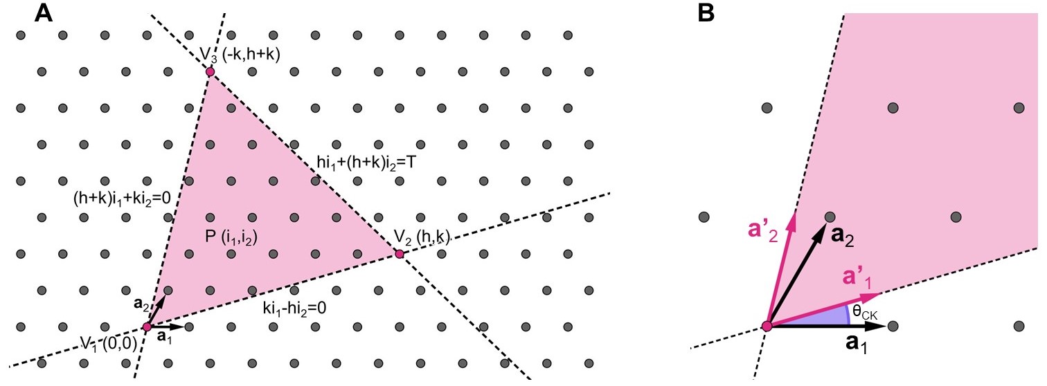
Figure S1: Implementation of the CK construction.
A Points belonging to the triangular face of the icosahedron are those enclosed by the three lines passing through the vertices, whose equations with respect to the basis primitive vectors $\mathbf{a}_{1}$ and $\mathbf{a}_{2}$ are reported in the figure. B Vectors $\mathbf{a}_{1}^{\prime}$ and $\mathbf{a}_{2}^{\prime}$, lying on two adjacent segment $V_{1}V_{2}$ and $V_{1}V_{3}$. $\mathbf{a}_{1}^{\prime}$ and $\mathbf{a}_{2}^{\prime}$ are obtained by rotating the primitive vectors $\mathbf{a}_{1}$ and $\mathbf{a}_{2}$ counterclockwise of an angle $\theta_{CK}$.

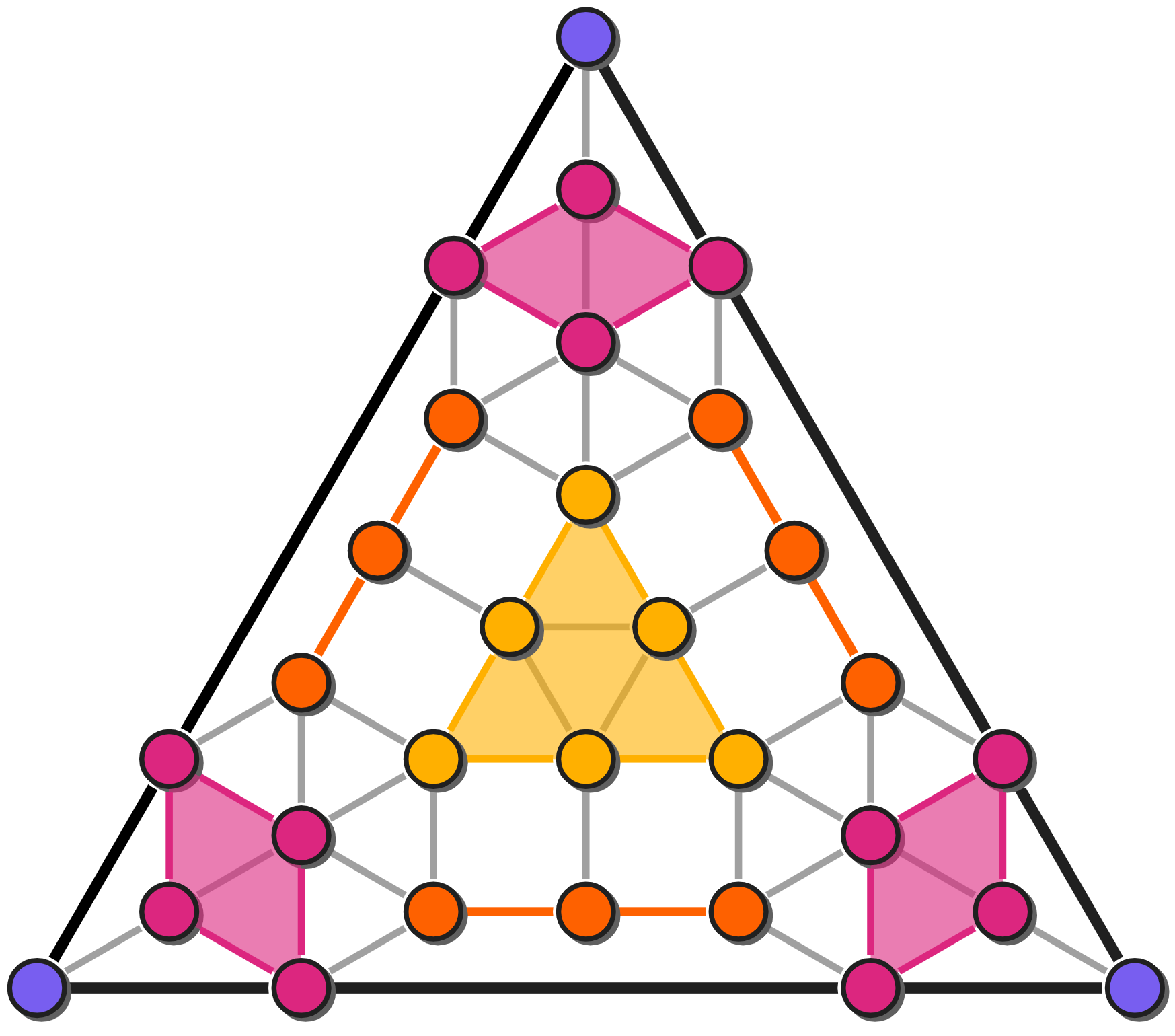
Figure S2: Facet of an anti-Mackay shell.
Particles are marked in different colours to help in counting the number of particles in the facet.

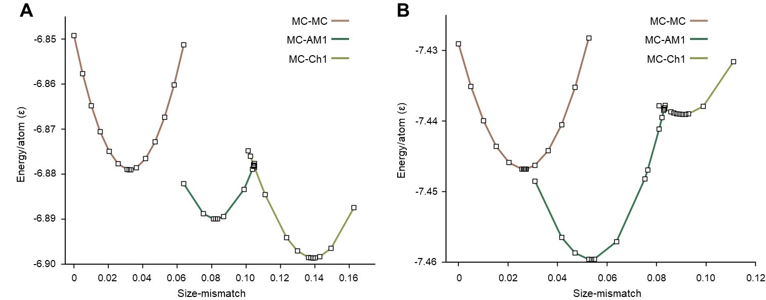
Figure S3: Stability of MC, AM1 and Ch1 shells in Lennard-Jones clusters.
Binding energy per particle (in $\varepsilon$ units) as a function of the size mismatch of A an icosahedron of $i=5$ MC shells covered by single MC, AM1 and Ch1 shells and B an icosahedron of $i=8$ MC shells covered by single MC, AM1 and Ch1 shells.

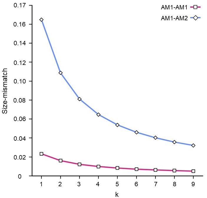
Figure S4: Optimal mismatch for two AM shells on a MC core.
A core terminated by a $(1,k)^{*}$ AM1 shell is covered by either a $(1,k+1)^{*}$ or a $(2,k)^{*}$ shell. The optimal mismatch is evaluated according to Eq. S82 and Eq. S83.

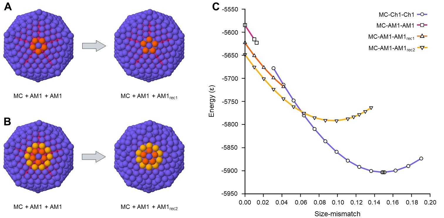
Figure S5: Stability of two AM shells on a MC core.
A-B The two types of reconstruction undergone by the outer AM1 shell spontaneously upon local minimization, involving rotations of particle rings around all vertices. C Energy (in $\varepsilon$ units) as a function of the mismatch for Lennard-Jones clusters made of 5 Mackay shells upon which two shells are added: two Ch1 shells; two AM1 shells; an AM1 shell plus a shell reconstructed as in A; an AM1 shell plus a shell reconstructed as in B.

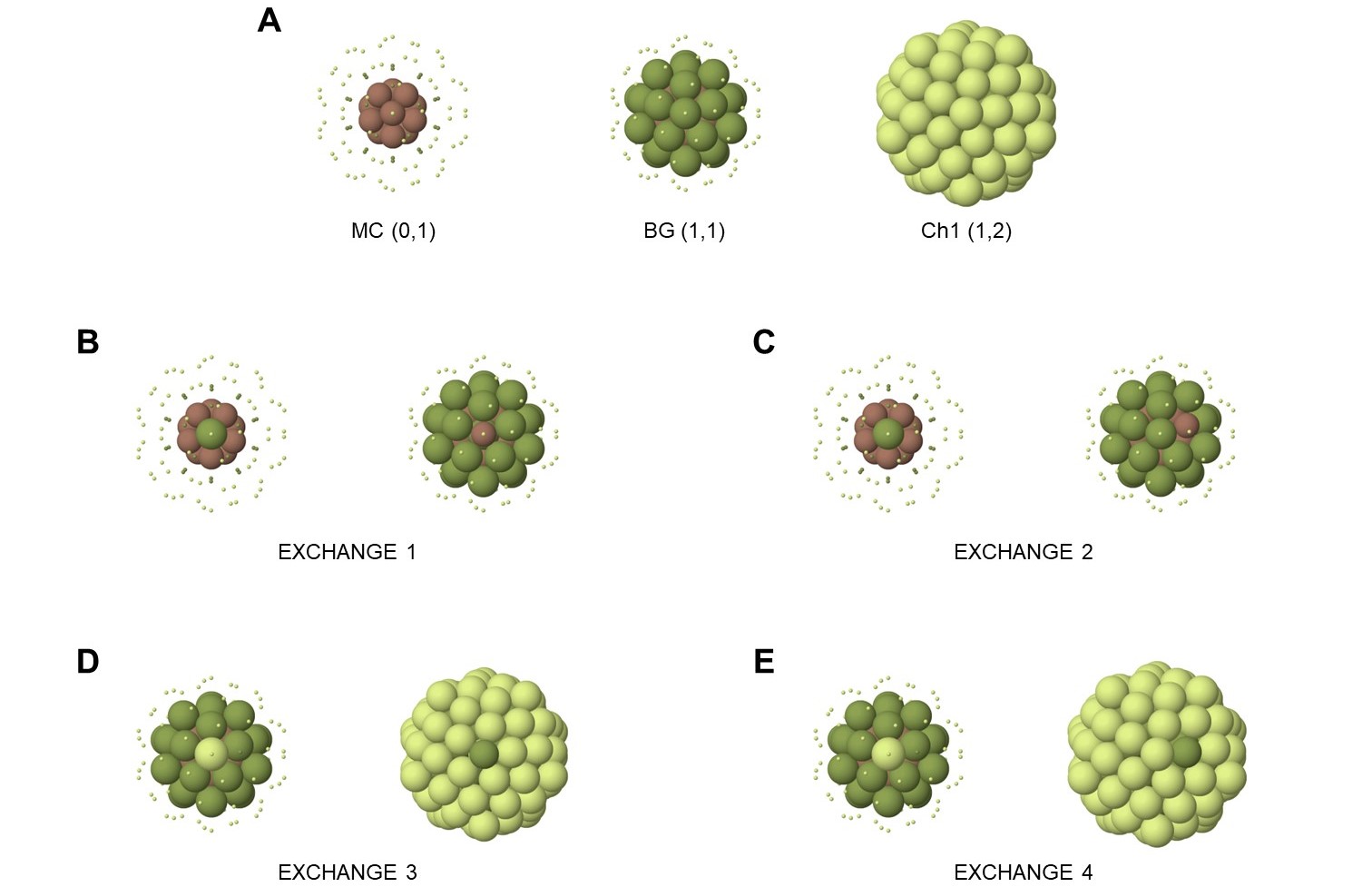
Figure S6: Clusters of the DFT calculations.
The structures considered in the calculations are of two types, with either $i=3$ or $i=4$ shells. In this figure we show only those containing BH and Ch1 shells, while the analogous structures containing 3 or 4 MC shells are not shown. The first structure ($i=3$) contains the central atom (0,0), the (0,1) MC shell, and the (1,1) BG shell, corresponding to the left and middle panels in A, for a total of 45 atoms. The second structure ($i=4$) contains in addition the (1,2) Ch1 shell, as shown in the right panel of A, for a total of 117 atoms. In B-E the different types of atom pair swaps are shown: in B and C between atoms of the (0,1) and (1,1) shells; in D and E between atoms of the (1,1) and (1,2) shells.

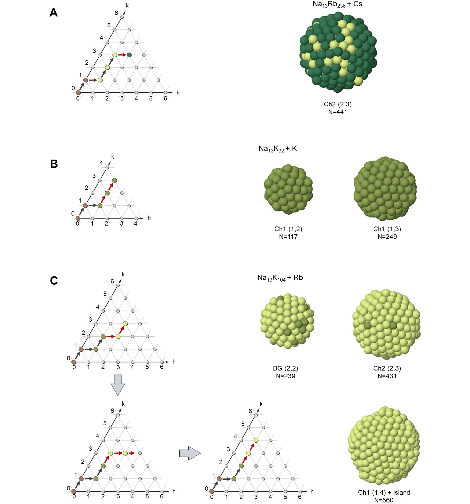
Figure S7: Growth simulations of alkali metal clusters.
A Deposition of Cs atoms on a Na@Rb seed of 249 atoms, in which a Mackay Na inner core is covered by two Ch1 shells of Rb atoms. The growth temperature is 125 K and the deposition rate is 1 atoms/ns. Cs atoms for a Ch2 shell. B Deposition of K atoms on a Na@K seed of 45 atoms, in which a Mackay core of 13 atoms is covered by one Ch1 shell of K atoms. The growth temperature is 125 K and the deposition rate is 1 atoms/ns. Deposited K atoms form two further Ch1 shells. C Deposition of Rb atoms on a Na@K seed of 117 atoms, made of a Mackay inner core of 13 Na atoms and two Ch1 shells of K atoms. Growth temperature is 125 K and deposition rate is 1 atoms/ns. Deposited Rb atoms first form the (2,2) BG shell, which is completed at 239 atoms, and then the growth continues by the formation of a (2,3) Ch2 shell. Upon deposition of further Rb atoms, the (2,2) shell suddenly transforms into a Ch1 (1,3) shell, still covered by a (2,3) Ch2 shell, which then transforms into a Ch1 (1,4) shell to finally reproduce the natural path which better corresponds to the optimal size mismatch between atoms of the different shells.

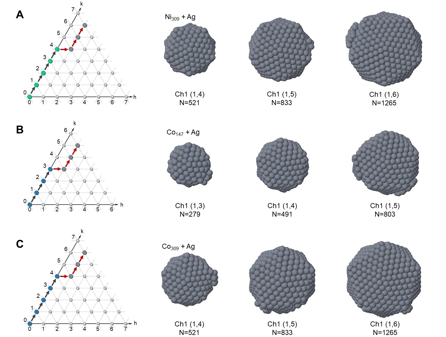
Figure S8: Growth sequences for Ag atoms on Ni and on Co seeds.
A Deposition of Ag atoms on a Ni₃₀₉ Mackay icosahedral seed, at $T=450$ K, and deposition rate 0.1 atoms$/$ns. B Deposition of Ag atoms on a Co₁₄₇ Mackay icosahedral seed, at $T=350$ K, and deposition rate 0.1 atoms$/$ns. c Deposition of Ag atoms on a Co₃₀₉ Mackay icosahedral seed, at $T=450$ K, and deposition rate 0.1 atom$/$ns. In A-C, we show the growth path (the part of the path corresponding to the red arrows) in the hexagonal lattice and images of the cluster surface at different growth stages.

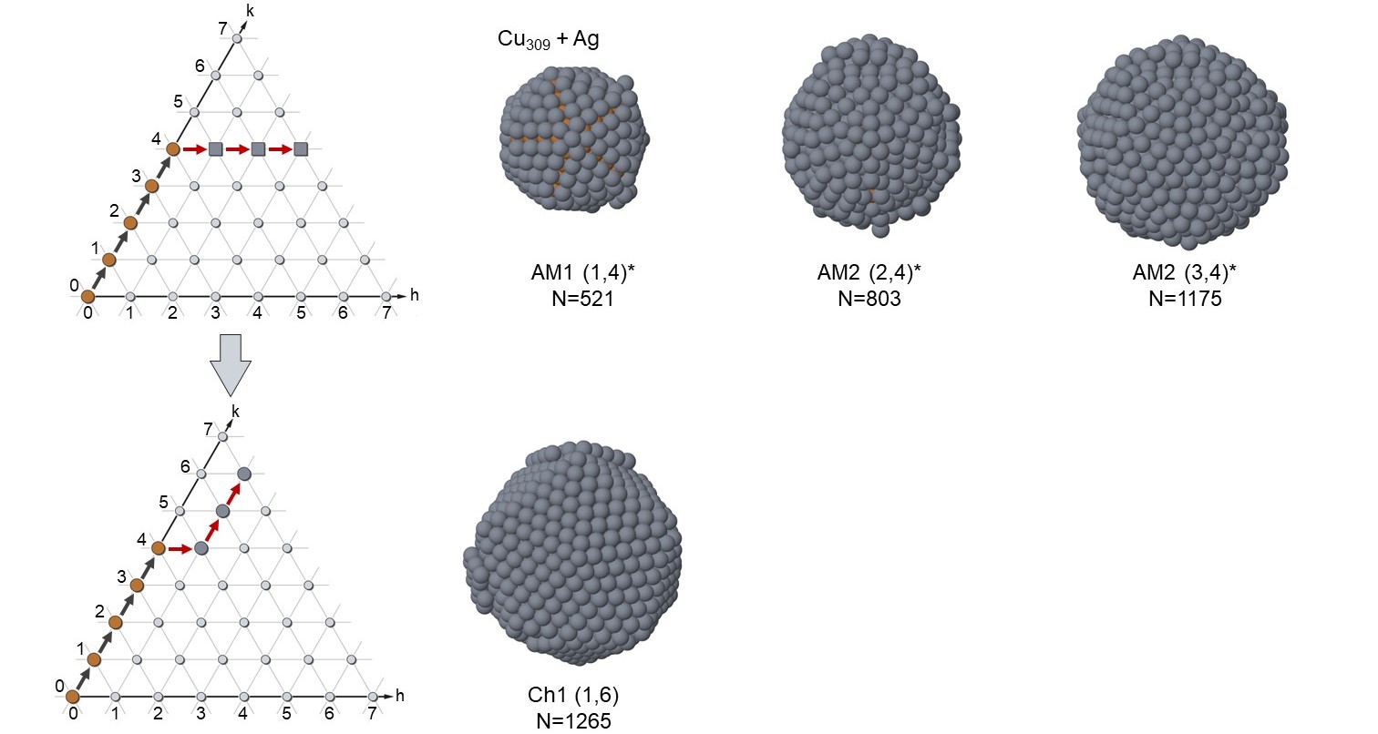
Figure S9: Growth sequence for Ag atoms on a Cu seed.
In the top row, the growth sequence is shown for the deposition of Ag atoms on a Cu₃₀₉ Mackay icosahedral seed, at $T=350$ K, and deposition rate 1 atom$/$ns up to size 1175. The growth produces AM structures changing class at each step in the hexagonal plane. The bottom row show the continuation of the growth up to size 1265. In this part of the simulation, a sudden rearrangement of the Ag shells to Ch1 structures takes place, so that the final structure does not contain AM shells anymore and its structure is represented by the the path in the bottom row. The sudden rearrangement is due to the very unfavourable energy of the AM multi-shell arrangement, which is highly metastable.

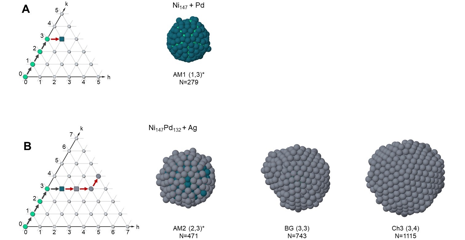
Figure S10: Growth sequence for AgPdNi clusters.
A Deposition of Pd atoms on a Ni₁₄₇ Mackay seed. Temperature 400 K, deposition rate 0.1 atoms/ns. An AM shell is formed. B Ag on a Ni₁₄₇@Pd₁₃₂ seed terminated by an AM1 shell. Temparature 300 K, deposition rate 0.1 atoms/ns. Ag atoms form an AM2 shell and then a defective BG shell. On top of the BG shell, a defective Ch3 shell grows.

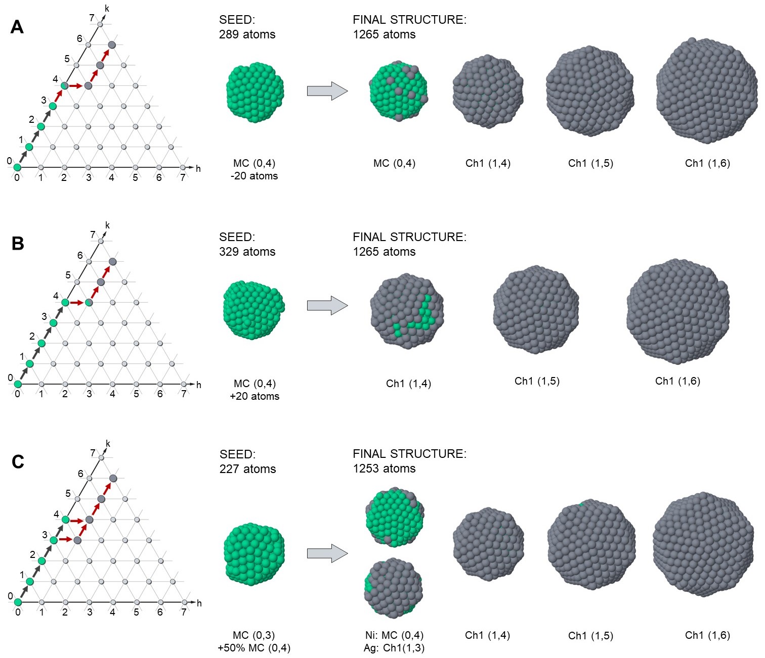
Figure S11: Growth of Ag atoms on a Ni defective seeds.
The growth simulations are at $T=450$ K, and deposition rate 0.1 atoms/ns. At variance with Figs. SS8 and SS9, here the images represent different shells of the final structures, obtained at the end of the growth, instead of snapshots taken during the growth. In A growth starts from a Ni₂₈₉ seed, which is terminated by a slightly incomplete (0,4) MC shell. in th efinal structure, the (0,4) shell is completed by Ag atoms, then covered by Ch1 shells. In B growth starts from a Ni₃₂₉ seed, which is terminated by a small fragment of a (0,5) MC shell. in the final structure, that shell is completed by Ag atoms, which transform it into a Ch1 (1,4) shell, which is covered by further Ch1 shells. In C the growth starts from a Ni₂₂₇ seed, which is terminated by a half (0,4) MC shell. in the final structure, that shell is completed by Ag atoms, so that a the resulting shell presents a Ni and an Ag half. On the Ni side, the shell is MC (0,4), while on the Ag side the shell is Ch1 (1,3). This is indicated by the bifurcation in the path. Further shells are of class Ch1.

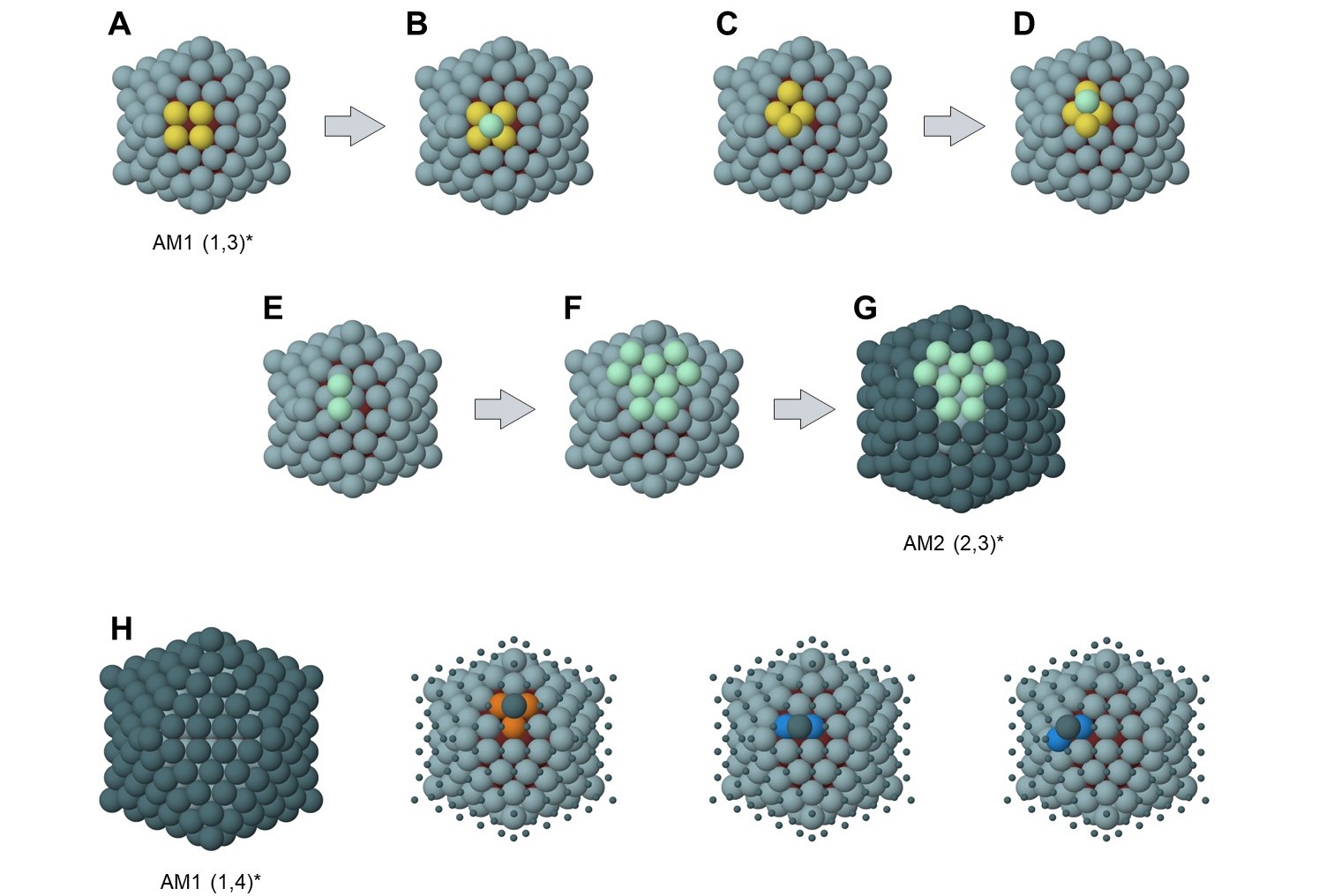
Figure S12: Growth mechanism on AM shells.
A The four orange atoms identify a fourfold adsorption site on the (1,3)^∗ AM shell. B A deposited adatom (cyan) is preferentially trapped in a site of this type. C A new fourfold adsorption site is created on top for the four orange atom so that D it can trap a further deposited atom. E-G The process is self-replicating, finally leading to the formation of the (2,3)^∗ AM shell. H The atoms of (1,4)^∗ AM shell on top of a (1,3)^∗ AM shell find only threefold adsorption sites, identified by the orange atoms. Sites at the facet edge are twofold (see the blue atoms) so that they are not even locally stable for isolated adatoms.

EXCH	3 SHELLS				4 SHELLS
	MC@BG		MC@MC		MC@(BG-Ch1)		MC@(MC-MC)
	DFT	GUPTA	DFT	GUPTA	DFT	GUPTA	DFT	GUPTA
1	+0.240	+0.322	$-0.345$	$-0.086$	+0.164	+0.251	$-0.046$	+0.013
2	+0.223	+0.262	$-0.323$	$-0.079$	+0.253	+0.273	$-0.064$	+0.006

Table 1: DFT and Gupta data for NaK clusters.
In the initial configurations, these clusters always contain a core with MC shells (0,0) and (0,1) made of Na atoms, while the other shells are made of K atoms. For MC@BG, the (1,1) BG shell is added to the core, whereas for MC@BG-Ch1 a further (1,2) shell is added (see Fig. S6)a). For MC@MC, the (0,2) shell is added to the core, whereas for MC@MC-MC a further (0,3) shell is added. Exchanges of type 1 and 2 (see Fig. S6b,c) are made on the initial configuration. The energy differences (in eV) between the configurations after and before the exchange of the atomic pair are reported. The exchange is favourable for negative differences, unfavourable otherwise.

EXCH	3 SHELLS				4 SHELLS
	MC@BG		MC@MC		MC@(BG-Ch1)		MC@(MC-MC)
	DFT	GUPTA	DFT	GUPTA	DFT	GUPTA	DFT	GUPTA
1	+0.283	+0.381	$-0.711$	$-0.415$	+0.205	+0.284	$-0.081$	$-0.024$
2	+0.237	+0.289	$-0.691$	$-0.395$	+0.293	+0.289	$-0.137$	$-0.045$

Table 2: DFT and Gupta data for NaRb clusters.
The same as in Table 1 but with Rb atoms instead of K atoms. Energies are in eV.

EXCH	MC@BG@Ch1		MC@MC@MC
	DFT	GUPTA	DFT	GUPTA
1	+0.180	+0.223	$-0.025$	+0.031
2	+0.242	+0.237	$-0.042$	$-0.006$
3	+0.064	+0.071	+0.031	+0.047
4	+0.048	+0.054	+0.019	+0.028

Table 3: DFT and Gupta data for NaKRb clusters.
In the initial configurations, these clusters always contain a core with MC shells (0,0) and (0,1) made of Na atoms, while the third and fourth shells are made of K and Rb atoms, respectively. For MC@BG@Ch1, the (1,1) and the (1,2) shells are added to the core (see Fig. S6)a), whereas for MC@MC@MC the (0,2) and (0,3) shells are added. Exchanges of types 1, 2, 3 and 4 (see Fig. S6b-e) are made on the initial configuration. The energy differences (in eV) between the configurations after and before the exchange of the atomic pair are reported. The exchange is favourable for negative differences, unfavourable otherwise.

References

- [1] Y. Yao, et al., Science 376, eabn3103 (2022).
- [2] Y. Yao, et al., Science Advances 6, eaaz0510 (2020).
- [3] P. Xie, et al., Nature Communications 10, 4011 (2019).
- [4] J. Yan, et al., Nature Communications 13, 2789 (2022).
- [5] P. D. Howes, R. Chandrawati, M. M. Stevens, Science 346, 1247390 (2014).
- [6] L. Chen, et al., Nature Communications 12, 4556 (2021).
- [7] D. Wang, et al., Nature Mater. 12, 81 (2013).
- [8] Q. Huo, et al., Journal of the American Chemical Society 128, 6447 (2006).
- [9] M. Vega-Paredes, et al., ACS Nano 17, 16943 (2023).
- [10] A. C. Foucher, et al., Chemistry of Materials 35, 8758 (2023).
- [11] D. Nelli, C. Roncaglia, C. Minnai, Advances in Physics: X 8, 2127330 (2023).
- [12] P. Strasser, et al., Nature Chem. 2, 454 (2010).
- [13] T. P. Martin, Phys. Rep. 273, 199 (1996).
- [14] F. Baletto, R. Ferrando, Rev. Mod. Phys. 77, 371 (2005).
- [15] D. L. D. Caspar, A. Klug, Cold Spring Harbor Symposia on Quantitative Biology 27, 1 (1962).
- [16] S. Li, P. Roy, A. Travesset, R. Zandi, Proceedings of the National Academy of Sciences 115, 10971 (2018).
- [17] R. Twarock, A. Luque, Nature Communications 10, 4414 (2019).
- [18] J. Farges, M. de Feraudy, B. Raoult, G. Torchet, Surface Science 106, 95 (1981).
- [19] Z. W. Wang, R. E. Palmer, Phys. Rev. Lett. 108, 245502 (2012).
- [20] M. R. Langille, J. Zhang, M. L. Personick, S. Li, C. A. Mirkin, Science 337, 954 (2012).
- [21] H. Hubert, et al., Nature 391, 376 (1998).
- [22] D. Nelli, et al., Nanoscale 15, 18891 (2023).
- [23] B. de Nijs, et al., Nature Materials 14, 56 (2015).
- [24] J. Wang, et al., Nature Communications 9, 5259 (2018).
- [25] Y. Chen, et al., Nature Physics 17, 121 (2021).
- [26] D. Shechtman, I. Blech, D. Gratias, J. W. Cahn, Phys. Rev. Lett. 53, 1951 (1984).
- [27] E. G. Noya, C. K. Wong, P. Llombart, J. P. K. Doye, Nature 596, 367 (2021).
- [28] A. A. Pankova, T. G. Akhmetshina, V. A. Blatov, D. M. Proserpio, Inorganic Chemistry 54, 6616 (2015).
- [29] M. G. Rossmann, J. E. Johnson, Annual Review of Biochemistry 58, 533 (1989).
- [30] D. Salunke, D. Caspar, R. Garcea, Biophys. J. 57, 887 (1989).
- [31] T. O. Yeates, M. C. Thompson, T. A. Bobik, Current Opinion in Structural Biology 21, 223 (2011).
- [32] R. Zandi, B. Dragnea, A. Travesset, R. Podgornik, Physics Reports 847, 1 (2020).
- [33] S. M. Douglas, et al., Nature 459, 414 (2009).
- [34] A. L. Mackay, Acta Crystallogr. 15, 916 (1962).
- [35] F. Sadre-Marandi, P. Das, Computational and Mathematical Biophysics 6, 1 (2018).
- [36] G. Bergman, J. L. Waugh, L. Pauling, Acta Cryst. 10, 254 (1957).
- [37] W. Branz, N. Malinowski, A. Enders, T. P. Martin, Phys. Rev. B 66, 094107 (2002).
- [38] K. Koga, K. Sugawara, Surf. Sci. 529, 23 (2003).
- [39] Y. Xia, D. Nelli, R. Ferrando, J. Yuan, Z. Y. Li, Nature Communications 12, 3019 (2021).
- [40] J. Wang, et al., ACS Nano 13, 9005 (2019).
- [41] P. Prinsen, P. van der Schoot, W. M. Gelbart, C. M. Knobler, The Journal of Physical Chemistry B 114, 5522 (2010).
- [42] E. Sasaki, D. Hilvert, The Journal of Physical Chemistry B 120, 6089 (2016).
- [43] R. L. Whetten, et al., Accounts of Chemical Research 52, 34 (2019).
- [44] A. Wang, J. Li, T. Zhang, Nature Reviews Chemistry 2, 65 (2018).
- [45] D. Bochicchio, R. Ferrando, Nano Lett. 10, 4211 (2010).
- [46] C. H. Bennett (1975). In Diffusion in Solids: Recent, Edited by A. S. Nowick and J. J. Burton. Academic Press, New York.
- [47] P. Giannozzi, et al., Journal of Physics: Condensed Matter 21, 395502 (2009).
- [48] J. P. Perdew, K. Burke, M. Ernzerhof, Phys. Rev. Lett. 77, 3865 (1996).
- [49] R. P. Gupta, Phys. Rev. B 23, 6265 (1981).
- [50] Y. Li, E. Blaisten-Barojas, D. A. Papaconstantopoulos, Phys. Rev. B 57, 15519 (1998).
- [51] F. Baletto, C. Mottet, R. Ferrando, Phys. Rev. B 66, 155420 (2002).
- [52] F. Baletto, C. Mottet, R. Ferrando, Phys. Rev. Lett. 90, 135504 (2003).
- [53] G. Rossi, G. Schiappelli, R. Ferrando, J. Comput. Theor. Nanosci. 6, 841 (2009).
Acknowledgments
The authors acknowledge the project PRIN2022 PINENUT of the Italian Ministry of University and Research. The authors thank Giovanni Barcaro, El yakout El koraychy, Alessandro Fortunelli, Alberto Giacomello, Laurence D. Marks, Richard E. Palmer, Emanuele Panizon, Michele Parrinello, Cesare Roncaglia, Giulia Rossi, Manoj Settem, Erio Tosatti and Jeffrey R. Weeks for a critical reading of the manuscript.