CHARME: A chain-based reinforcement learning approach for the minor embedding problem
Abstract.
Quantum Annealing (QA) holds great potential for solving combinatorial optimization problems efficiently. However, the effectiveness of QA algorithms heavily relies on the embedding of problem instances, represented as logical graphs, into the quantum unit processing (QPU) whose topology is in form of a limited connectivity graph, known as the minor embedding Problem. Existing methods for the minor embedding problem suffer from scalability issues when confronted with larger problem sizes. In this paper, we propose a novel approach utilizing Reinforcement Learning (RL) techniques to address the minor embedding problem, named CHARME. CHARME includes three key components: a Graph Neural Network (GNN) architecture for policy modeling, a state transition algorithm ensuring solution validity, and an order exploration strategy for effective training. Through comprehensive experiments on synthetic and real-world instances, we demonstrate that the efficiency of our proposed order exploration strategy as well as our proposed RL framework, CHARME. In details, CHARME yields superior solutions compared to fast embedding methods such as Minorminer and ATOM. Moreover, our method surpasses the OCT-based approach, known for its slower runtime but high-quality solutions, in several cases. In addition, our proposed exploration enhances the efficiency of the training of the CHARME framework by providing better solutions compared to the greedy strategy.
1. Introduction
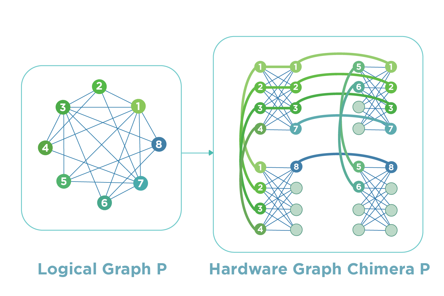
Quantum annealing (QA) is a quantum-based computational approach that leverage quantum phenomena such as entanglement and superposition to tackle complex optimization problems, in various domains such as machine learning (Pudenz and Lidar, 2013),(Caldeira et al., 2019),(Mott et al., 2017), bioinformatics (Mulligan and et al, 2019), (Fox and et al, 2022), (Ngo et al., 2023b), and networking (Guillaume and et al, 2022), (Ishizaki, 2019). QA tackles optimization problems through a three-step process. First, the problem is encoded using a logical graph which represents the quadratic unconstrained binary optimization (QUBO) formulation of a given problem. Next, the logical graph is embedded into a Quantum Processing Unit (QPU), which has its own graph representation known as hardware graph. The embedding aims to ensure that the logical graph can be obtained by contracting edges in the embedded subgraph of the hardware graph. This embedding process is commonly referred to as minor embedding. Finally, the quantum annealing process is repeatedly executed on the embedded QPU to find an optimal solution for the given problem.
In this process, the minor embedding arises as a major bottleneck that prevents quantum annealing from scaling up. In particular, the topology of the hardware graph or its induced subgraphs may not perfectly align with that of the logical graph; therefore, minor embedding typically requires a significant number of additional qubits and their connections to represent the logical graph on the hardware graph. Consequently, this situation can lead to two primary issues that can degrade the efficiency of quantum annealing. First of all, the need for a significant number of additional qubits to embed the logical graph can strain the available resources of the hardware graph, leading to the scalability issues in term of limiting hardware resources. Furthermore, when the size of the logical graph increases, the running time required to identify a feasible embedding increases exponentially. As a result, quantum annealing with a prolonged embedding time can be inefficient in practical optimization problems, which require rapid decision-making.
In the literature, there are two main approaches to address the above challenges in minor embedding, namely top-down and bottom-up. The top-down approach aims to find embeddings of complete graphs (Choi, 2011), (Klymko et al., 2012), (Boothby et al., 2016) in the hardware graph. While embedding a complete graph can work as a solution for any incomplete graph with the same or smaller size, the embedding process for incomplete graphs, especially sparse graphs, usually requires much fewer qubits compared to embedding a complete graph. As a result, the top-down approach may not be the most effective strategy for embedding sparse logical graphs. Although post-process techniques have been considered to mitigate this problem (Goodrich et al., 2018), (Serra et al., 2022), handling sparse graphs is a huge hindrance to the top-down approach.
On the other hand, the bottom-up approach directly constructs solutions based on the topology of the logical and the hardware graphs. This approach involves computing minor embedding through either Integer Programming (IP) which finds an exact solution from predefined constraints (Bernal et al., 2020), or progressive heuristic methods which gradually map individual nodes of the logical graph to the hardware graph (Cai et al., 2014), (Pinilla and Wilton, 2019), (Ngo et al., 2023a). Compared to the top-down approaches, bottom-up methods are not constrained by the pre-defined embedding of complete graphs, allowing for more flexible embedding constructions. However, bottom-up approaches need to consider a set of complicated conditions associated to the minor embedding problem (which we will explain later). As a result, the computational cost required to obtain a feasible solution is substantial.
In order to overcome the above shortcomings, we introduce a novel learning approach based on the Reinforcement Learning (RL). Leveraging its learning capabilities, RL can rapidly generate solutions for previously unseen problem instances using its well-trained policy, thus efficiently enhancing the runtime complexity. Furthermore, through interactions with the environment and receiving rewards or penalties based on the quality of solutions obtained from the environment, RL agents can autonomously refine their strategies over time. This enables them to explore state-of-the-art solutions, particularly beneficial for emerging and evolving challenges such as minor embedding. Thus, RL is commonly applied to solve optimization problems in quantum systems (Khairy et al., 2020; Chen et al., 2022; Wauters et al., 2020; Fan et al., 2022; Ostaszewski et al., 2021).
Although RL has emerged as a powerful technique for handling optimization problems (Bengio et al., 2021), applying it to our minor embedding problem has encountered several challenges. The first challenge is the stringent feasibility requirement for solutions in the minor embedding problem. Specifically, feasible solutions must fulfill a set of conditions for the minor embedding problem including chain connection, global connection and one-to-many. These constraints lead to an overwhelming number of infeasible solutions, compared to the number of feasible ones within the search space. As a result, it is challenging for the RL framework to explore adequate number of feasible solutions during the training phase as well as the testing phase.
The second challenge lies in the policy design of the RL framework. In particular, the policy of the RL framework is a parameterized structure which receives the information derived from the current state as the input, and return the decision for the next state. In each step, the policy is queried to determine the next state. Thus, the efficiency of the RL framework heavily depends on the design of the policy which specifies the processing of state’s information. For example, a structure that extract uncorrelated relations from state’s information can hinder the convergence of the policy. In addition, the minor embedding problem considers two independent graphs which must be included in the state’s information. However, exploiting the relations between two graphs which are meaningful to the minor embedding problem is challenging. Therefore, there is a need for an efficient policy structure which can capture valuable relations in state’s information to facilitate the process of training policy’s parameters.
To realize an RL-based approach for the minor embedding problem, we first introduce an initial design, named NaiveRL, which sequentially embeds each node in a given logical graph into an associated hardware graph. Based on this initial design, we further introduce CHARME, incorporating three key additional components, to tackle the aforementioned challenges. The first component is a GNN-based architecture, which integrates features from the logical graph, the hardware graph, and the embedding between the two graphs. This integration allows the architecture to return action probabilities and state values, serving as a model for the policy in the RL framework. The second component is a state transition algorithm which sequentially embed a node in the logical graph into a chain of nodes in the hardware graph in order to ensure the validity of the resulting solutions. Lastly, the third component is an order exploration strategy that navigates the RL agent towards areas in the search space with good solutions, facilitating the training process.
Our proposed solutions are further evaluated extensively against three state-of-the art methods, including OCT-based, a top-down approach (Goodrich et al., 2018), and two bottom-up approaches Minorminer (Cai et al., 2014) and ATOM (Ngo et al., 2023a). The results illustrate that CHARME outperforms all state-of-the-art methods in term of qubit usage for very sparse logical graphs. In addition, the computational efficiency of CHARME is comparable to that of the fastest method in terms of the running time.
Organization. The rest of the paper is structured as follows. Section 2 introduces the definition of minor embedding and an overview of reinforcement learning. Our method and its theoretical analysis are described in Section 3. Section 4 presents our experimental results. Finally, section 5 concludes the paper.
2. Preliminaries
This section formally defines the minor embedding problem in the quantum annealing and presents the preliminaries needed for our proposed solutions. It includes a brief overview of ATOM for the minor embedding problem based on a concept of topology adaption (Ngo et al., 2023a), basic concepts of reinforcement learning, and Advantage Actor Critic (A2C) (Mnih et al., 2016), which will be partially adopted in our solution.
2.1. Minor Embedding Problem
| Notion | Definition |
|---|---|
| Power set of set . | |
| Logical graph with the set of nodes and the set of edges . | |
| The adjacency matrix and the node feature matrix of . | |
| Hardware graph with the set of nodes and the set of edges . | |
| The adjacency matrix and the node feature matrix of . | |
| Induced subgraph of for set of nodes . | |
| The embedding from to at the step . | |
| Total size (the number of qubits) of , calculated by . | |
| The set of nodes in that are embedded to at the step . | |
| The set of nodes in that are embedded by a node in at the step . | |
| The embedding order including different precomputed actions. . | |
| can be considered as a permutation of the set . | |
| The space of embedding orders which are permutations of the set . | |
| The space of embedding orders which are permutations of the set | |
| with the prefix . |
We first present fundamental concepts and terminologies needed to understand how QA solves optimization problems. Next, we describe the minor embedding problem in QA. The common terminologies used throughout this paper are described in Table 1.
Given an optimization problem with a set of binary variables and quadratic coefficients , the problem can be represented in a QUBO form as follows:
| (1) |
From this equation, we express the optimal solution for the given problem corresponding to the state with lowest energy of final Hamiltonian as such that for :
| (2) |
The QUBO formulation is then encoded using a graph called logical graph. In the logical graph, each node corresponds to a binary variable . For any two nodes and , there exists an edge if the quadratic coefficient is nonzero.
The hardware graph is a representation of the topology of QPU with nodes corresponding to qubits and edges corresponding to qubits’ couplers. QA system of D-Wave consists of three QPU topologies, namely Chimera - the earliest topology, Pegasus - the latest topology, and Zephyr - next generation QPU topology. These topologies are all in a grid form: a grid of identical sets of nodes called unit cells. In this paper, we consider the Chimera topology. The reason is that embedding methods in Chimera topology may be translated to Pegasus topology without modification, because Chimera is a subgraph of Pegasus (Boothby et al., 2020). In other words, the method which we develop for Chimera model also works for Pegasus topology.
QUBO models a given optimization problem as a logical graph, and the topology of QPU used in QA as a hardware graph. In order to solve the final Hamiltonian which QA processes, we need to find an mapping from the logical graph to the hardware graph. Below we formally define the minor embedding problem:
Definition 0.
Given a logical graph and a hardware graph , minor embedding problem seeks to find a mapping function satisfying three embedding constraints:
-
(1)
Chain connection: We denote a subset of nodes in that are mapped from a node in as chain . , any subgraph of induced by a chain from is connected.
-
(2)
Global connection: For every edge , there exists at least one edge such that and .
-
(3)
One-to-many: Two chains and in the hardware graph do not have any common nodes with .
We note that an embedding which satisfies the above three embedding constraints is referred as a feasible solution.
2.2. Heuristic approaches for the minor embedding problem
In this part, we provide an overview of heuristic solutions for the minor embedding problem, especially focused on ATOM (Ngo et al., 2023a).
Heuristic methods employ a step-by-step approach to construct solutions. In the work of Cai et al.(Cai et al., 2014), each step involves embedding a selected node from the logical graph into a suitable set of nodes in the hardware graph, while satisfying specific conditions. This iterative process continues until a feasible embedding is obtained. However, this method can encounter a problem when no appropriate set exists for the selected node. We call it isolated problem. To address this issue, the latest heuristic method, called ATOM(Ngo et al., 2023a), introduces an adaptive topology concept. Given a logical graph and a hardware graph , this method consists of three main phases to find a feasible embedding from to :
-
(1)
Initialization: A solution is initialized as , and an embedded set is initialized as . In addition, an permutation of nodes in the logical graph, denoted by , is precomputed heuristically. This permutation is consider as a node order to guide the embedding process, where each node in the logical graph is iteratively embedded into a chain of nodes in the hardware graph.
-
(2)
Path construction: In this phase, we iteratively embed nodes in into following the order of through steps. Specifically, in the step , the node is selected. Then, an algorithm, named NODE EMBEDDING, is designed to find a new embedding such that combination of and is a feasible embedding for . If exists, is updated with . This step is repeated for the subsequent in the order until is empty. Otherwise, in cases where a feasible embedding cannot be obtained for node , it indicates the occurrence of an isolated problem. In such situations, phase 3 is triggered to handle this problem.
-
(3)
Topology adaption: This phase is to handle the isolated problem. An algorithm, named TOPOLOGY ADAPTING, is introduced to expand the current embedding to a new embedding in such a way that the isolated problem no longer occurs. Then, it returns to phase 2 where is replaced by .
ATOM method guarantees to return a feasible solution after at most steps. In addition, NODE EMBEDDING and TOPOLOGY ADAPTING algorithms have low computational complexity. Thus, ATOM can achieve an efficient performance in practice. However, one limitation of this approach is that the heuristic strategy used to determine the embedding order may not be optimized, that can lead to a higher number of required qubits.
2.3. Reinforcement Learning
Reinforcement learning is a framework for addressing the problem of a RL-Agent learning to interact with an environment, formalized as a Markov Decision Process (MDP) , where is the set of possible states, is the set of possible actions, is the transition function, is the reward function, and is a discount factor that determines the importance of future rewards. In this framework, the RL-Agent and the environment interact at discrete time steps. At the time step , the RL-Agent observes a state from the environment. Subsequently, the RL-Agent selects an action based on a policy which is defined as a probability distribution over actions for each state, i.e., is the probability of taking action given the state . Upon taking action , the RL-Agent receives a reward and transitions to a new state according to the transition function . The policy is updated based on the observed interactions between the RL-Agent and the environment.
There are several methods for updating the policy. In the policy-based reinforcement learning, the policy is parameterized and updated directly using classical optimizers (i.e. gradient descent). On the other hand, the value-based reinforcement learning, instead of directly learning the policy , learns to estimate the state-value function which is calculated as the expected sum of discounted future rewards given a policy . Subsequently, the policy for action selection is updated in a greedy manner based on the state-value function. The state-value function is expressed as follows:
| (3) |
Following this approach, it is common to use the action-value function or Q-function, denoted as , which represents the expected cumulative reward if the RL-Agent chooses action under the current state and the policy . Given the state obtained by taking the action under the state , the Q-function is presented as follows:
| (4) |
Recently, hybrid approaches leverage the advantages of both policy-based and value-based techniques by concurrently learning both a policy and a state-value function. One prominent method in this approach is the Actor-Critic method which is essential for addressing the exploration-exploitation trade-off problem in reinforcement learning. In the Actor-Critic paradigm, two key models are employed: the Actor, parameterized by , which predicts the policy , and the Critic, parameterized by , which predicts the state value function . The Policy Gradient algorithm is commonly utilized to update the parameters and . The objective function employed in the Policy Gradient method is expressed as follows:
| (5) |
3. Proposed Solutions
In this section, we initially present our baseline RL framework, called NaiveRL, and CHARME, our advanced solution (Sect. 3.1). The three key components of CHARME are introduced in subsequent sections 3.2-3.4 along with its theoretical analysis.
3.1. RL framework
In this part, we first present NaiveRL which is an initial RL framework for the minor embedding problem. In this framework, solutions are constructed by sequentially mapping one node from a given logical graph to one node in a hardware graph. This approach gives an initial intuition of how to formulate an optimization problem by an RL framework. We then identify drawbacks of this framework which corresponds to challenges mentioned before. Accordingly, we introduce CHARME, a chain-based RL framework which effectively addresses the above drawbacks of NaiveRL. Unlike NaiveRL, CHARME constructs solutions by sequentially mapping one node from a given logical graph to a chain of nodes in a hardware graph. By doing this, CHARME is able to maintain the satisfaction of three embedding constraints after each step of embedding, thereby ensuring the feasibility of the resulting solutions.
3.1.1. NaiveRL - An Initial RL framework
We consider a simple RL framework which constructs solutions by sequentially embedding one node in logical graph to one unembedded node in the hardware graph . The algorithm terminates when the found solution satisfies three embedding constraints: chain connection, global connection, and one-to-many connection. Alternatively, it stops if there is no remaining unembedded node in . We define the states, actions, transition function and reward function in the RL framework as follows:
States: A state is a combination of the logical graph , the hardware graph , and a embedding . Specifically, we denote a state at step as .
Actions: An action is in form of with and . Note that is an unembedded node which is not in current embedding . The action is equivalent to embedding node in to an unembedded node in .
Transition function: When an action is taken, a new solution with is obtained. The new state is a combination of logical graph , hardware graph , and the new solution .
Reward function: At a step , the reward for selecting an action consists of two terms. The first term, named Verification , is determined based on the quality of resulting solution after taking an action . Specifically, if the solution satisfies all three embedding constraints, is a number of actions taken to reach that state (which is equivalent to ). Otherwise, is set to 0.
In addition, to address the challenge of sparse rewards caused by the large search space, we introduce an additional component for the reward function, named Exploration . This component is designed to encourage the RL framework to initially learn from existing solutions before independently exploring the search space. In particular, is calculated by the difference between the action found by our NaiveRL framework at step , denoted as , and the action found by an existing step-by-step heuristic method (Ngo et al., 2023a) at step , denoted as . The extent to which exploration contributes to the reward function is controlled by a variable . In the initial stages of the training phase, we set the variable as 0. It implies that in the early steps of training, the policy of the RL framework mimics the heuristic strategy. As the policy is progressively updated with precomputed solutions, gradually decreases in proportion to the agent’s success rate in finding solutions that satisfy the three embedding constraints. To sum up, the reward function for a given state can be expressed as follows:
| (6) |
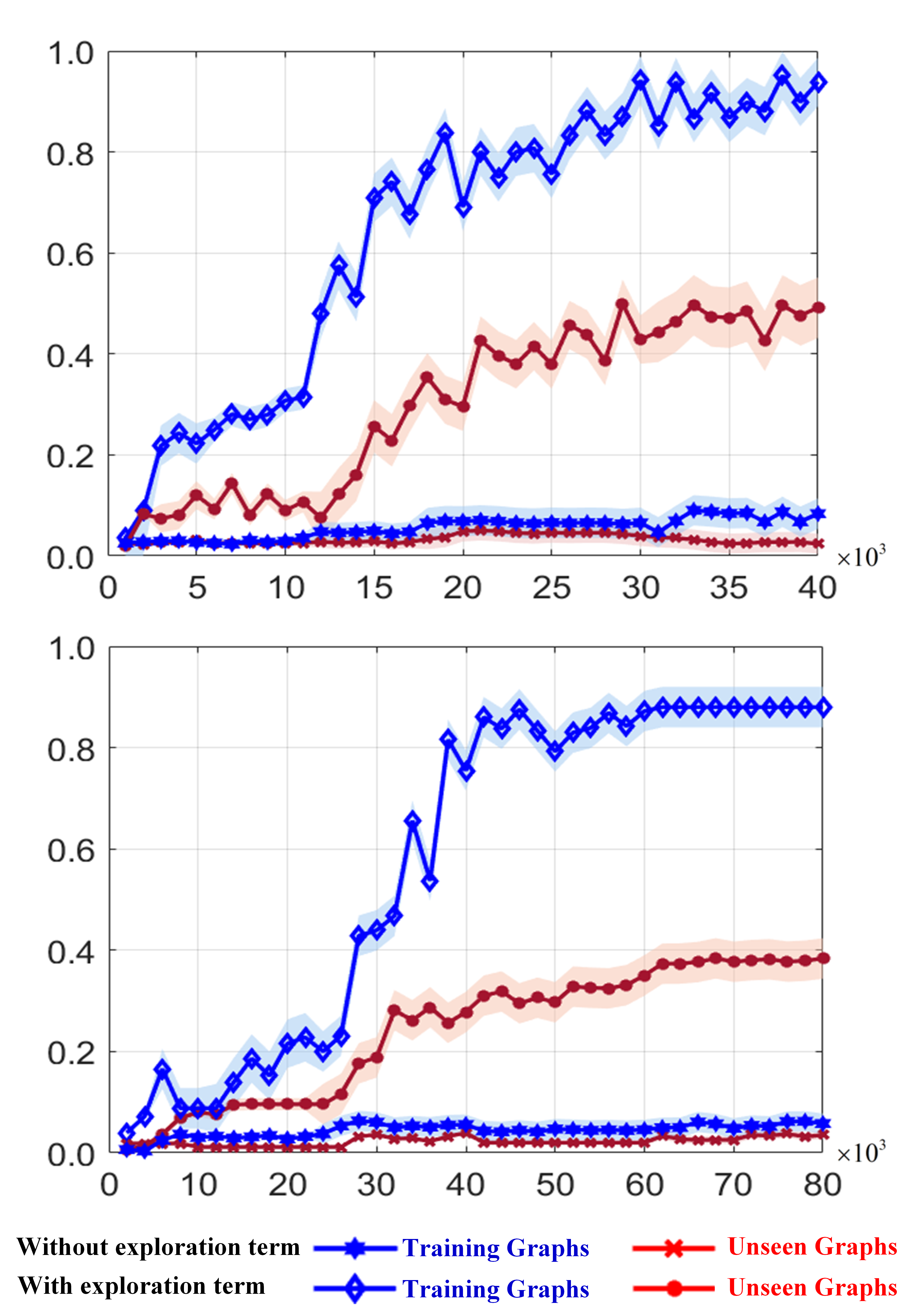
Limitations of NaiveRL. Here, we assess the practical performance of NaiveRL, in order to identify its limitations. First, we generate a dataset of 1000 graphs and split them into training and test sets. Our goal is to train the model on 700 Barabási-Albert (BA) graphs with nodes and degree with the aim of enabling effective generalization to the remaining 300 graphs with various sizes () and a lower degree (). Figure 2 illustrates the limitation in the generalization ability of NaiveRL. Without the exploration term in Equation 6, the model faced difficulties in finding feasible solutions. Despite an improvement achieved by adding the exploration term in Equation 6, the model is still struggling to generalize effectively to unseen graphs. Furthermore, there is no guarantee that NaiveRL can consistently generate feasible solutions, even with further training. This presents a bottleneck in the quantum annealing process, as feasible solutions are always necessary. As a result, there is a need for an enhanced and efficient RL framework design that can generalizes its policy for unseen graphs and ensure the feasibility of resulting solutions.
3.1.2. CHARME: A chain-based RL solution for the minor embedding problem
To overcome the limitations of NaiveRL, we introduce our proposed CHARME, a chain-based RL framework that embeds one node in the logical graph into a chain of nodes in the hardware graph at each step. CHARME guarantees to find feasible solutions within exact steps. Consequently, compared to the naive approach, the chain-based RL framework significantly reduces and simplifies the search space. In the following, we describe the chain-based RL framework.
States: We use the same definition of states in the former framework. Here, we specify components of states in more details. The state at step contains:
-
•
The logical graph : We represent the logical graph as a tuple . indicates the adjacency matrix of . Given the number of node features as , indicates the node feature matrix of . We specify the node features of later.
-
•
The hardware graph : We represent the logical graph as a tuple . indicates the adjacency matrix of . Given the number of node features as , indicates the node feature matrix of . We specify the node features of later.
-
•
The solution/embedding: We denote as an embedding from to at step . Specifically, if a node is embedded onto a node , then .
Actions: At step , we denote as a set of embedded node in . In each step, In each step, an action is defined as choosing an unembedded node . From here, for simplicity, we consider each action as an unembedded node of . Based on , we can find the next feasible embedding of in .
Transition function: Because the given graphs and remain unchanged throughout an episode (which is explained later), we consider a transition from state to state as the transition from to . The algorithm for state transition will be discussed in the subsequent section.
Reward function: At step , a reward for selecting a node is determined based on two components. The first component is the qubit gain compared to the current embedding, denoted as . This component can be computed as the difference between the number of qubits of and . The second component is the exploration term which is similarly defined as that in the reward function of NaiveRL, with the difference being that the precomputed solution is obtained through our proposed exploration algorithm, which we will discuss later. This component plays a role in facilitating the training process of the chain-based RL framework. To sum up, the reward is defined as follows:
| (7) |
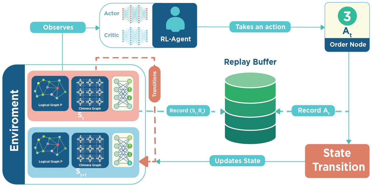
In order to describe the workflow of CHARME, first of all, we denote a round of finding a solution for a pair of as an episode. Given a training set of logical and hardware graphs, CHARME runs multiple episodes to explore solutions of pairs of logical and hardware graphs from the training set. In one episode, the framework constructs a solution through a series of steps. Figure 3 shows the workflow of CHARME in a step . Specifically, at step of an episode, CHARME receives the state including the logical graph, the hardware graph and the corresponding embedding, as inputs. The RL-Agent uses its policy to map the given state to an appropriate action , leading to the next state (Note that the policy of the RL-Agent is also the policy of the RL framework). In our CHARME, we apply the Actor-Critic method (Mnih et al., 2016) for our policy. The actor and the critic are represented by two different models with a similar structure which is explained later. Next, the state transition algorithm takes current state and chosen action as inputs to produces the next state . Finally the environment updates state to , and calculates the reward . Information in step including states, actions, and rewards is stored in a roll-out buffer which is later used for updating the RL-Agent’s policy. The episode continues until the RL-Agent reaches the terminal state where no unembedded node remains.
It is observable that for each episode, the RL-Agent explores an embedding order for a training pair . By learning from reward signals along with embedding orders, CHARME is able to generate efficient embedding orders for unseen logical graphs and hardware graphs, consequently reducing the qubit usage.
3.2. Graph representation and the structure of the policy
In this section, we present an efficient representation of logical and hardware graphs and introduce a GNN-based structure for the models representing the policy.
As we mentioned in the former section, the logical graph at step is presented by a tuple . In this work, we use the constant feature matrix for all logical graph . On the other hand, the hardware graph presented by a tuple . Specifically, the feature of a node in corresponds to the logical node embedded in . If node is unembedded, the feature of is .
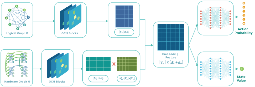
Based on the representation of and , we propose a GNN-based structure for models representing the RL-Agent’s policy (Figure 4). Specifically, this structure is applied for the actor and the critic in the RL-Agent. The structure receives an input as a tuple of and returns the action probability (for the actor) and state value (for the critic). The flow of the structure starts with passing the representations of and through GNN layers. GNN layers are powerful for learning and analysing graph-structured data, so they are capable of extracting information from the logical and hardware graphs which is essential for the minor embedding problem. Subsequently, given the numbers of GNN output features corresponding to and as and respectively, we obtain updated feature vectors and which are aggregation of topological information and initial features.
| (8) |
| (9) |
We then group nodes in that belong to the same chain in and aggregate their features. In order to accomplish that, we present as a matrix such that for , if and only if . As a result, we obtain the aggregated features as follows:
| (10) |
This step is important for several reasons. First of all, it eliminates unembedded nodes in the hardware graph. The information related to unembedded nodes is considered redundant because, given a fixed hardware topology, the position of unembedded nodes can be inferred from the embedded nodes. Hence, the information of embedded nodes alone is sufficient to make the decision about the next action. As a result, filtering out unembedded nodes significantly reduces computational costs without hindering the convergence of the policy’s parameters. On the other hand, the information of nodes embedded in the same chain is aggregated. After the aggregation, the output serves as the features of chains in the hardware graph.
Next, we concatenate and to obtain the final embedding feature . Subsequently, fully connected layers are applied to transform into the desired output. The dimension of these layers varies depending on whether the desired output is the action probability or the state value.
We observe that the final embedding feature , which combines the information from the logical graph , the hardware graph , and the corresponding embedding , has dimensions. Thus, our proposed architecture addresses the challenge of the state processing by efficiently combining the information from the graphs and the embedding.
3.3. State transition algorithm
We now present a state transition algorithm that computes the next state based on the current state and action. This algorithm integrates with the NODE EMBEDDING and TOPOLOGY ADAPTING algorithms introduced in (Ngo et al., 2023a).
Algorithm 1, referred to as STATE TRANSITION algorithm, takes current state at the time step including current logical graph , current hardware graph and current embedding , as well as an action as inputs. It produces the next state including the logical graph , the hardware graph and next embedding .
Before explaining this algorithm in details, we recall the set of embedded node as which can be inferred from . Algorithm 1 must guarantee that the resulting next embedding is a feasible embedding of into . To accomplish that, in details, first we initialize the decision variable as True (line 2) and assign as (line 3). Then, the node is embedded into the current hardware graph by finding an additional embedding through NODE EMBEDDING algorithm. If the additional embedding is not empty ( is successfully embedded), Algorithm 1 constructs new embedding by combining and (line 7). Besides, it updates new features for the hardware graph following a hardware representation which we discuss in the previous section (line 8). The next state is a combination of logical graph , hardware graph with updated features, and new embedding . In the end, we assign the value of as False, finish the loop and return the new state . Otherwise, if , we cannot embed the node with current embedding. We call this phenomenon as isolated problem. In order to overcome this bottleneck, we expand current embedding by TOPOLOGY ADAPTING algorithm (line 11), and repeat the whole process until we find a satisfied additional embedding .
From the lemmas provided in the work (Ngo et al., 2023a), it can be proven that assuming the current embedding is feasible, the next embedding of the subsequent state returned by Algorithm 1 is a feasible embedding of in . Additionally, the empty embedding initialized at step 0 is a feasible embedding of the empty logical graph in . Consequently, considering , we can recursively infer that the final embedding corresponding to the terminal state obtained in the -th step is a feasible embedding of in . Hence, with the state transition algorithm, our CHARME effectively addresses the challenge of ensuring feasibility.
3.4. Exploration Strategy
A challenge our proposed RL model needs to address is its efficiency when training with large instances. Specifically, as the number of nodes in the training logical graphs increases, the number of possible action sequences grows exponentially. Consequently, it becomes more challenging for the model to explore good action sequences for learning, potentially leading to an inefficient policy. In CHARME, we handle this issue by incorporating an exploration term in the reward function as Equation 7. The philosophy behind the exploration term is that at beginning training steps, when the policy is still developing, the model aims to replicate precomputed actions from an existing method. Subsequently, as the policy undergoes sufficient updates, the model gradually reduces its reliance on precomputed actions and begins to explore by itself. By doing that, the model can jump into a region with good solutions at the beginning and start to explore from that region, making the training more efficient.
Precomputed actions can be extracted from the solutions of the embedding method in the work (Ngo et al., 2023a). However, that method focuses on providing a fast minor embedding, so the sequence of precomputed actions are not carefully refined. In this section, we propose a technique to explore efficient sequences of precomputed actions in training logical graphs, making the training process more efficient. To avoid confusion, from here, we mention the sequences including precomputed actions as embedding orders. We name our proposed technique as Order Exploration.
3.4.1. Overview
Given a logical graph with and a hardware graph , an embedding order with results in a set of embeddings . As mentioned in previous sections, given an embedding step , the embedding is constructed by inputting Algorithm 1 with and for . We note that the construction of may require the topology expansion (i.e. the function is triggered). We call embeddings that require topology expansion as expansion embeddings. Otherwise, we call them as non-expansion embeddings. The expansion and non-expansion notions are used later in this section. In addition, we denote as the efficiency score of . Order Exploration aims to fast find emebedding orders for training logical graphs such that their efficiency scores are as small as possible.
The overview of Order Exploration is described in Algorithm 2. Algorithm 2 takes the inputs as the set of given training logical graphs, denoted as , the set of rescaling constants , the sampling limit and the exploration limit . The training graph includes the set of nodes and the set of edges . Given a logical graph , we define the embedding order as the sequence of precomputed actions for the training graph . We can see that the position of an action in is the step in which the action is embedded in the hardware graph, so from here, we mention the index of actions in as the embedding step. The goal of Algorithm 2 is to fast explore embedding orders for logical training graphs, denoted as , such that their efficiency scores are as small as possible.
In general, Algorithm 2 randomly picks a graph and explore the order for . In details, first, we initialize embedding orders corresponding to training graphs in (line 1). Specifically, given a graph , we initialize as a random permutation of the set . Then, we assign each graph with an equal potential score (line 2). These scores indicate the potential of being further improved for embedding orders.
After initialization, we start to update embedding orders within steps. For each step, a graph is sampled from the set based on the distribution for potential scores (line 4). Specifically, the selection probability is given as follow:
| (11) |
Afterward, we calculate the efficiency score of (line 5). Then, we refine the order by the subroutine Order Refining which is discussed later (line 6). In general, Order Refining aims to find an order such that its efficiency score is lower than in exploration steps. The number controls the running time of this subroutine. In addition, Order Refining returns as if a better order is found (line 7). If so, we update as (line 8), recalculate the efficiency score and update the potential score as follows:
| (12) |
Here, we can select the rescaling constant as the total number of qubits used for embedding resulting from an existing embedding method. Thus, the score , calculated by Equation 12, give us the gap between our refined solution and the existing solution. Consequently, the larger the gap is, the higher the likelihood that the corresponding graph will be selected for further refinement. It is also worth noting that if the initial potential scores are sufficiently large, every graph can be selected at least once.
When the algorithm finishes discovering, it returns all feasible orders through the set (line 11).
3.4.2. Order Refining
We observe that an embedding order is a permutation of , so the space of embedding orders for is equivalent to the group of permutations of . Therefore, finding embedding orders with low efficiency score from this space is challenging. To address this issue, first, we establish an estimated lower bound on the efficiency scores for a special family of embedding orders. Then, based on the lower bound, we propose the subroutine Order Refining for fast exploring orders, described in Algorithm 3.
Before going further in details, we introduce notions used in this section. Given a set , we define as the group of permutations of . From this, we infer that the space for embedding orders of is . We also refer to an order as a complete order. Considering two disjoint sets and , we define the concatenation operator on the two groups and as the symbol . Specifically, given two orders and , we have . In addition, considering an order , we denote the group of complete orders with prefix as . Specifically, an order is formed as where .
Next, we consider a special prefix type, named non-expansion prefix. Given a subset with , and a prefix , we say that is a non-expansion prefix if all orders , results in a set of embeddings such that with , is non-expansion embedding.
Now, we consider constructing the embedding order by iteratively selecting an action as a node in and appending its to the current order. Each step for action selection is denoted as an embedding step. At the embedding step , we assume that the embedding order is a non-expansion prefix. In other word, the topology is no longer expanded from the embedding step . Theorem 1 gives us the comparison between the number of qubits gained when selecting an action at the embedding steps and in this setting.
Theorem 1.
Given a hardware graph and a logical graph with , assume that at the embedding step , we have the sequence of selected actions as a non-expansion prefix. We prove that given a node , the number of qubits required to embed at the step is not greater than that required when embedding at the step .
Proof.
First, we set up notions we use in this proof. We denote the embedding at the embedding step as . Specifically, the embedding is constructed by embedding actions with each action as a node in the logical graph . At the embedding step , we denote the set of nodes in which are already embedded into the hardware as , while we denote the set of nodes in which are embedded by a node in the logical graph as . We note that the set is equivalent to .
We define a path in the hardware graph as where is the path length. We consider a path as a clean path at the time if with and with . From that, we denote the set of all possible clean paths in the embedding step as . Given a hardware node and an logical node , we denote the set of all clean path from to the chain as . Note that if . Then, we denote the shortest clean path at the embedding step from to as
| (13) |
At the embedding step , given an unembedded logical node , we denote the number of qubits gained for embedding into as . From Algorithm 1, we find the an unembedded hardware node such that the size of the union of shortest clean paths from to chains of neighbors of is minimized. Thus, denoted the set of neighbors of in the logical graph as , we can calculate as follows:
| (14) |
Next, we consider embedding the node the embedding step . We assume that an arbitrary set of actions is embedded in intermediate embedding steps such that . We update the set and based on the assumption that there is no expansion embedding between the embedding step and . Then, we establish the relation between and . First, we observe that . Thus, we imply that following by for . As a result, from Equation 13, we have . Then, based on Equation 14, given an unembedded node , we have:
Therefore, the theorem is proven.
∎
Based on Theorem 1, given a non-expansion prefix , we establish the lower bound on the efficiency score of all embedding orders as follows:
| (15) |
Later, in the experiment, we show that for general prefix , Theorem 1 is still valid for most of pairs and , proving the usefulness of the lower bound in general.
Then, we propose a subroutine for exploring embedding orders, described in Algorithm 3. Algorithm 3 takes a training logical graph with , the hardware graph , the current embedding step , the prefix order , the number of recursive steps and the qubit threshold . Its goal is to find an suffix such that the efficiency score of is less than within recursive steps. Specifically, Algorithm 3 returns a message variable , the suffix and the number of remaining recursive steps . The message variable indicates whether a feasible suffix is found. If is equal to , is assigned as .
Here, we provide a detailed explanation of Algorithm 3. First, we reconstruct embeddings based on Algorithm 1 (line 1 - 4). If there is no more node to consider (), Algorithm 3 compares the efficiency score of the complete embedding order with the threshold to return appropriate message variable (line 5 - 9). Then, we calculate the estimated lower bound based on Equation 15 (line 10 - 15). If , Algorithm 3 stops the current recursion (line 16 - 17). Finally, a random node is picked and the next recursion at the embedding step is triggered with the updated prefix and the number of remaining recursive steps (line 19 - 23). The subroutine, which is triggered at the embedding step , can return a complete embedding order with the efficiency score less than .
4. Experiments
This section presents our experimental evaluation with two focuses: 1) confirming the efficiency of our proposed exploration strategy, and 2) comparing the performance of our end-to-end RL framework, CHARME, to three state-of-the-art methods: OCT-based (Goodrich et al., 2018), Minorminer (Cai et al., 2014), and ATOM (Ngo et al., 2023a) in terms of the number of qubits used, and the total running time.
4.1. Setup
Dataset. We conduct our experiments on synthetic and real datasets. For the synthetic dataset, we generate logical graphs using Barabási-Albert (BA) model. In details, we split the synthetic dataset into a training set and a testing set. The training set, denoted as , includes 700 BA graphs with nodes and degree , while the testing set includes 300 new graphs which are generated by varying the number of nodes and the degree . The hardware graph used in this experiment is in form of Chimera topology which is a grid of unit cells (Boothby et al., 2016). The experiment on the synthetic dataset aims to evaluate the performance of CHARME on logical graphs from the same distribution.
Furthermore, we also conduct the experiments on the real dataset which is generated based on the QUBO formulations of test instances of the Target Identification by Enzymes (TIE) problem proposed in the work (Ngo et al., 2023b). In particular, different metabolic networks for the TIE problem result in different QUBO formulations. As we mentioned in previous sections, each specific QUBO formulation corresponds to a logical graph. Thus, we can generate various logical graphs by varying the metabolic networks for the TIE problem. In this experiment, we collect 105 metabolic networks from the KEGG database (Kanehisa and Goto, 2000). Then, we generate corresponding logical graphs by using the QUBO formulations with these metabolic networks as input. In collected graphs, the number of nodes ranges from 6 to 165, while the number of edges ranges from 22 to 578. We split the dataset into three groups based on the ratio between the number of nodes , and the number of edges : low density group (), medium density group (), and high density group (). We use 70 graphs for training, and preserve the remaining for testing. We denote the training set . This experiment aimed to illustrate the effectiveness of our hybrid RL model in real-world scenarios.
Benchmark. To demonstrate the effectiveness of our Order Exploration strategy, we establish a comparative greedy strategy referred to as Greedy Exploration. Greedy Exploration approach explores the embedding orders based on the algorithm.
Then, we proceed to compare the performance of our end-to-end framework, CHARME, with three state-of-the-art methods for the minor embedding problem, as outlined below:
-
•
OCT-based (Goodrich et al., 2018): This method follows the top-down approach that minimizes the number of qubits based on their proposed concept of the virtual hardware framework. In this experiment, we use the most efficient version of OCT-based, named Fast-OCT-reduce. While the OCT-based is effective in reducing the number of qubits, it suffers from high computational complexity, leading to long running time to find a solution. This can pose a bottleneck for quantum annealing process, especially when frequency of quantum annealing usage has been increased rapidly.
-
•
Minorminer (Cai et al., 2014): This method is a heuristic method developed commercially by D-Wave. This method finds solutions by adding nodes of a logical graph to the hardware graph sequentially. Minorminer is an efficient approach for sparse logical graphs.
-
•
ATOM (Ngo et al., 2023a): This method is a heuristic method which finds solutions based on the concept of adaptive topology. The strength of this method is the ability to find solutions in small running time without compromising their quality. The concept of adaptive topology is integrated in CHARME through the state transition algorithm. Thus, by comparing its performance to that of ATOM, we can assess the effectiveness of RL in leveraging a heuristic method.
Hyper-parameter selection. In the exploration phase, we apply Exploration Order, described in Algorithm 2, to precompute embedding orders for each graph . Specifically, we set the sampling as , the exploration limit as and use up to threads running in parallel for exploring embedding orders.
For training, the method for GNN layers in both actor and critic models is graph convolutional networks (Kipf and Welling, 2017). Each model has three GNN layers. The learning rate for the actor model is , while the learning rate for the critic model is . The number of episodes to update policy is , and the batch size in each update is .
For inference, due to the stochastic in behaviours of machine learning models, we sample solutions for each testcase, and report the solution with the least number of qubits. In addition, we use multi-processing for sampling solutions, so the actual running time of inference is equal to the time to sample one solution.
4.2. Results
4.2.1. The performance of the proposed exploration strategy
This section demonstrates the utility of Order Exploration in generating precomputed actions, commonly referred to as embedding orders, to streamline the training process of CHARME. Our experiments are designed to assess two key aspects: 1) the effectiveness of Theorem 1 with general prefix that implies the the practical significance of the lower bound outlined in Equation 15, and 2) the overall performance of our proposed exploration strategy in terms of the efficiency scores of resulting embedding orders.
| 80 | 100 | 120 | 140 | |||||||||
|---|---|---|---|---|---|---|---|---|---|---|---|---|
| d | 2 | 5 | 10 | 2 | 5 | 10 | 2 | 5 | 10 | 2 | 5 | 10 |
| Early embedded gain | 5.36 | 14.09 | 17.15 | 6.01 | 15.28 | 23.19 | 6.28 | 17.75 | 30.66 | 7.07 | 21.78 | 36.85 |
| Late embedded gain | 8.94 | 18.73 | 25.70 | 11.57 | 22.81 | 34.62 | 12.20 | 29.14 | 56.02 | 17.75 | 38.72 | 67.02 |
The effectiveness of Theorem 1 with general prefix. In this experiment, we designed a meticulous procedure to evaluate the effectiveness of Theorem 1 for general prefix orders which are not necessarily non-expansion. Specifically, we compare the number of qubits gained when embedding a same node at two different embedding steps and , denoted as and . In Theorem 1, we prove that if there is no expansion embedding between and . Thus, our focus here lies on comparing and when at least one expansion embedding exists between these steps. Given a graph , the procedure for selecting , , and unfolds as follows. First, we randomly select a subset following by selecting a random prefix . We select as a random node in . Next, we need to select and such that there exists one expansion embedding from to . In details, we start with iteratively embedding nodes following the prefix order . Subsequently, we randomly embed nodes until we obtain an expansion embedding at step . Finally, is assigned as and is randomly selected such that . By repeatedly performing this procedure, we can obtain different , , and for each training graph. For each triplet of a given training graph, and is calculated similarly as discussed in Theorem 1. For each setting of , we measure the average of and on all triplet sampled from graphs with the setting . We denote the average on and as early embedded gain and late embedded gain respectively.
The results are illustrated in Table 2. Across all configurations, the average qubit requirement for embedding a node prior to topology expansion (early embedded gain) is consistently lower compared to post-topology expansion (late embedded gain). Interestingly, when the graph’s density increases, the difference in qubit gain between before and after topology expansion become more significant. This trend can be attributed to the expansion of the topology, which, on average, elongates the length of clean paths. Consequently, embedding a node after topology expansion tends to incur higher costs. These observations highlight the significance of the lower bound on the efficiency score of embedding orders with a general prefix, as derived from Equation 15.
The efficiency in exploring orders. In this experiment, we conducted a comparison between Order Exploration and Greedy Exploration to assess their effectiveness in exploring embedding orders for training logical graphs across various node sizes and degrees . Figure 5 presents subfigures corresponding to each setting of logical graphs in the synthetic training set . Each subfigure showcases the efficiency scores of embedding orders resulted from both strategies with variations in the exploration limit which is mentioned in Algorithm 2. We recall that given a logical graph and a hardware graph , the efficiency score of an embedding order is the number of qubits when embedding into following the order .
The results depicted in the subfigures highlight the superior performance of Order Exploration over Greedy Exploration across all settings. In detals, the disparity becomes more significant with increasing values of and . For example, with , the average efficiency score of Order Exploration is approximately less than that of Random Exploration, while with , the gap increases to around . Furthermore, we observe that the disparity also widens as the exploration limit increases from to . The key difference between two methods is the lower bound derived from Theorem 1. Thus, by these results, we assert the practical utility of Theorem 1 in guiding the exploration of embedding orders, particularly in scenarios involving large values and high exploration limits .
Similarly, when applied to the real training set , the Order Exploration approach consistently outperforms Greedy Exploration in terms of efficiency scores (Figure 6). Specifically, when dealing with low-density and medium-density graphs, we observe that the disparity between Order Exploration and Greedy Exploration is small. This is because the small number of nodes and edges limit the available options for embedding orders. However, when dealing with high-density graphs, Order Exploration significantly outperforms Greedy Exploration. Specifically, Order Exploration requires approximately qubits, while Greedy Exploration requires more than qubits for its solution. This illustrates the superior performance of Order Exploration, particularly in settings involving high-density graphs.
4.2.2. The performance of CHARME
In this experiment, we compare the performance of CHARME against three state-of-the-art methods in the synthetic and real datasets.
n 80 100 120 140 degree 2 5 10 2 5 10 2 5 10 2 5 10 OCT-based 357.76 845.38 1222.11 515.74 1263.32 1850.9 725.84 1782.18 2607.06 931.24 2348.74 3488.18 Minorminer 338.56 1236.88 2110.16 501.56 1914.18 3313.24 664.76 2632.82 4854.10 830.56 3554.01 6573.84 ATOM 384.06 1126.14 1815.72 546.62 1782.86 2882.72 727.46 2560.36 4217.48 998.58 3448.24 5621.88 CHARME 324.62 1027.36 1686.20 485.16 1580.08 2566.14 655.88 2263.66 3870.02 821.88 3082.59 5100.54
The synthetic dataset. Here, we assess the performance of CHARME approach in the synthetic dataset, focusing on the number of qubits used and the running time. The goals of this experiment are as follows:
-
•
We evaluate how effectively CHARME framework leverages the heuristic method ATOM.
-
•
We compare the quality of solutions in terms of the number of qubits obtained by CHARME approach with three state-of-the-art methods.
-
•
We measure the inference time of CHARME approach and compare it with the running time of other methods to assess its computational efficiency.
Table 3 presents the average number of qubits obtained from solutions generated by four methods for various pairs of size and degree of logical graphs. First of all, the results imply that CHARME leverages the heuristic strategy used in ATOM. Across all pairs , CHARME consistently provides solutions with fewer qubits compared to ATOM. In particular, CHARME achieves 11.36% reduction in qubit usage compared to ATOM. This observation not only indicates the efficiency of the proposed CHARME framework, but it also illustrates the generalization ability of the RL framework because the policy learnt from the training set can perform well for new graphs with different sizes and degrees.
Turning to solution quality, the results in Table 3 demonstrate an out-performance three state-of-the-art methods in term of qubit usage in test cases with degree . On average, in these cases, CHARME achieves 2.52% of reduction in term of qubit usage, compared to current best methods. In other cases, although CHARME cannot overcome the OCT-based in term of qubit usage, it still outperforms Minorminer and ATOM. This observation, combined with the subsequent analyse of running time is important to illustrate the practical effectiveness of CHARME in handling the minor embedding problem.
Finally, we examine the running time of four methods. The results in Figure 7 illustrate that the running time of OCT-based is significantly larger than the running time of three other methods. In particular, the running time of OCT-based is approximately 6 times bigger than the running time of the second slowest method, Minorminer. Thus, although OCT-based is efficient in term of qubit usage in some certain cases, its expensive running time can pose a significant bottleneck in practical quantum annealing process. On the other hand, the running time of CHARME is comparable to the fastest method, ATOM. Furthermore, as we mentioned above, CHARME can offer better solutions than Minorminer and ATOM in all cases. Therefore, CHARME can be the optimal choice for tackling minor embedding problem in practice, especially when current quantum annealers must handle user requests immediately due to the raising demand on their utilization.
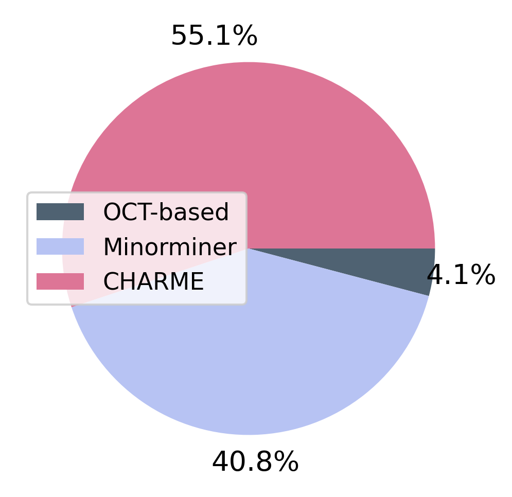
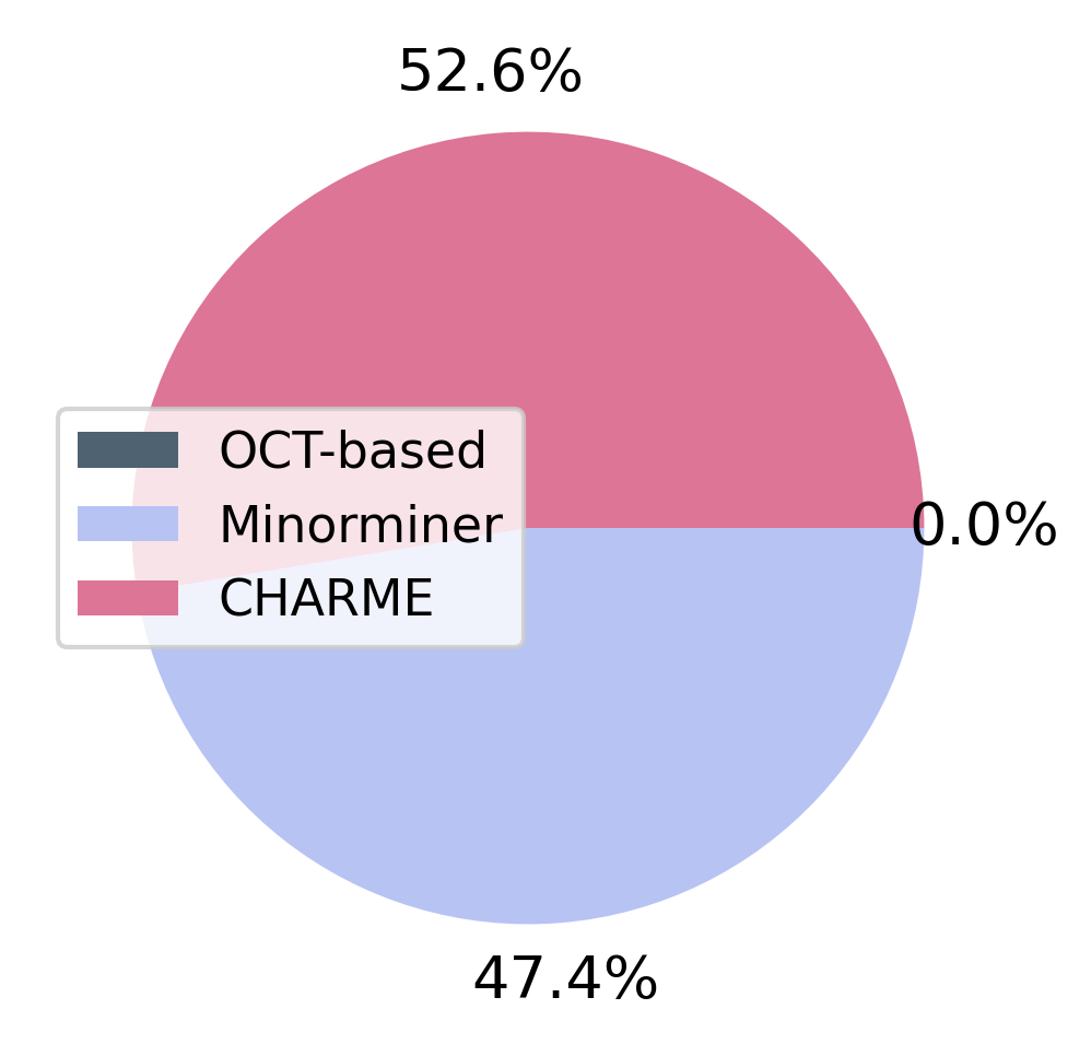
The real dataset. Here, we assess the performance of CHARME in comparison to OCT-based and Minorminer in a real dataset. To evaluate these methods, we measure the frequency at which each approach achieves the best solutions across three testing groups: low density, medium density, and high density. Additionally, we analyze the running time of the three methods for various sizes of graphs.
Figure 8 illustrates the frequency of finding the best solutions in term of qubit usage of three methods for various testing groups including low density, medium density and high density. First, the CHARME method consistently outperforms the competitors, achieving the highest frequency of finding solutions with the fewest qubits in all three testing groups. Remarkably, the frequency of CHARME method is always above 50%, illustrating its superiority. Another interesting observation is in the performance of the OCT-based method which works well on the synthetic dataset, but struggles on the actual QUBO-based dataset. This phenomena is due to the sparse nature of logical graphs formed by actual QUBO formulation, making top-down approaches like Minorminer and CHARME more efficient choices.
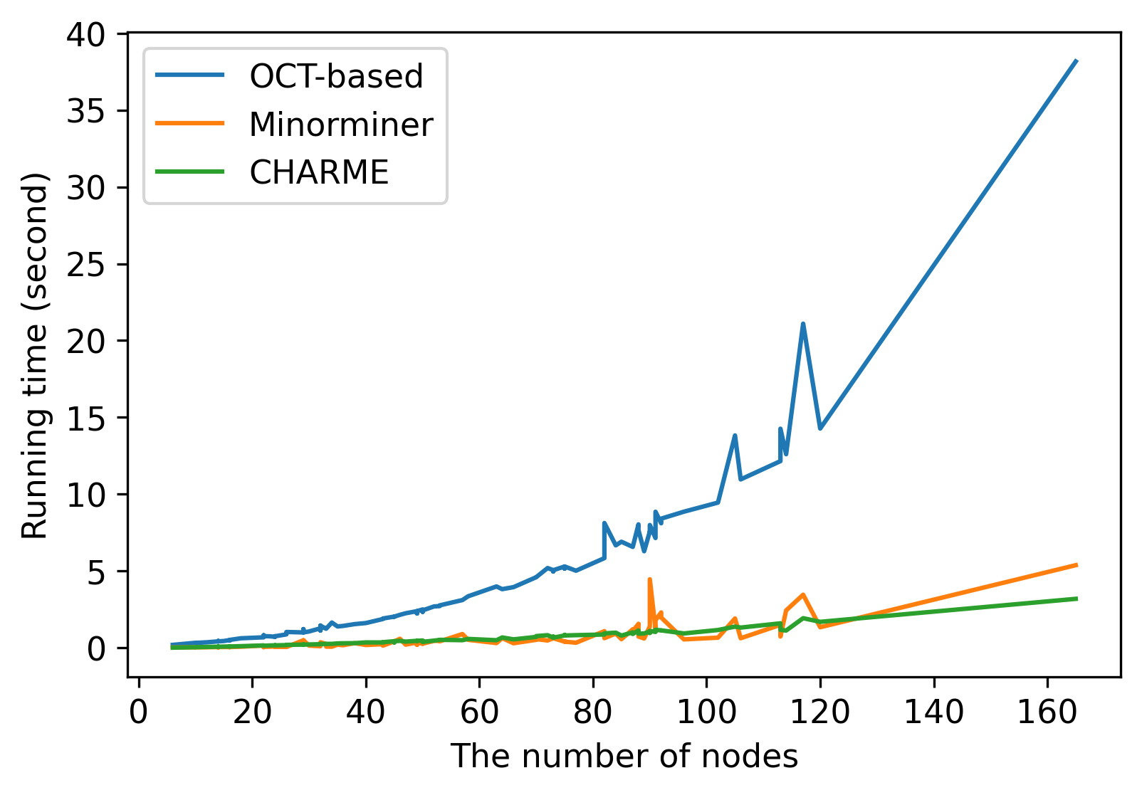
On the other hand, Figure 9 presents the running time analysis of the three methods. We observe a similar trend in the running time for the real-world dataset compared to the synthetic dataset. Specifically, the running time for Minorminer and CHARME method is comparable, while the OCT-based method exhibits significantly higher running times. That further confirms the efficiency of top down approaches in handling the real world dataset. In addition, the running time line of CHARME is smoother than lines of Minorminer and OCT-based which exhibit some fluctuations. This observation suggests that CHARME’s performance is more stable compared to its competitors.
5. Conclusion
In conclusion, our work introduces CHARME, a novel approach using Reinforcement Learning (RL) to tackle the minor embedding Problem in QA. Through experiments on synthetic and real-world instances, CHARME demonstrates superior performance compared to existing methods, including fast embedding techniques like Minorminer and ATOM, as well as the OCT-based approach known for its high-quality solutions but slower runtime. Additionally, our proposed exploration strategy enhances the efficiency of CHARME’s training process. These results highlight the potential of CHARME to address scalability challenges in QA, offering promising avenues for future research and application in quantum optimization algorithms.
References
- (1)
- Bengio et al. (2021) Yoshua Bengio, Andrea Lodi, and Antoine Prouvost. 2021. Machine learning for combinatorial optimization: A methodological tour d’horizon. European Journal of Operational Research 290, 2 (2021), 405–421. https://doi.org/10.1016/j.ejor.2020.07.063
- Bernal et al. (2020) David E. Bernal, Kyle E. C. Booth, Raouf Dridi, Hedayat Alghassi, Sridhar Tayur, and Davide Venturelli. 2020. Integer Programming Techniques for Minor-Embedding in Quantum Annealers. In Integration of Constraint Programming, Artificial Intelligence, and Operations Research. Cham, 112–129.
- Boothby et al. (2020) Kelly Boothby, Paul Bunyk, Jack Raymond, and Aidan Roy. 2020. Next-Generation Topology of D-Wave Quantum Processors. https://doi.org/10.48550/ARXIV.2003.00133
- Boothby et al. (2016) Tomas Boothby, Andrew D. King, and Aidan Roy. 2016. Fast clique minor generation in Chimera qubit connectivity graphs. Quantum Information Processing 15, 1 (01 Jan 2016), 495–508. https://doi.org/10.1007/s11128-015-1150-6
- Cai et al. (2014) Jun Cai, William G. Macready, and Aidan Roy. 2014. A practical heuristic for finding graph minors. https://doi.org/10.48550/ARXIV.1406.2741
- Caldeira et al. (2019) João Caldeira, Joshua Job, Steven H. Adachi, Brian Nord, and Gabriel N. Perdue. 2019. Restricted Boltzmann Machines for galaxy morphology classification with a quantum annealer. (14 Nov 2019). https://www.osti.gov/biblio/1594136 Research Org.: Fermi National Accelerator Lab. (FNAL), Batavia, IL (United States).
- Chen et al. (2022) Samuel Yen-Chi Chen, Chih-Min Huang, Chia-Wei Hsing, Hsi-Sheng Goan, and Ying-Jer Kao. 2022. Variational quantum reinforcement learning via evolutionary optimization. Machine Learning: Science and Technology 3, 1 (feb 2022), 015025. https://doi.org/10.1088/2632-2153/ac4559
- Choi (2011) Vicky Choi. 2011. Minor-embedding in adiabatic quantum computation: II. Minor-universal graph design. Quantum Information Processing 10, 3 (01 Jun 2011), 343–353. https://doi.org/10.1007/s11128-010-0200-3
- Fan et al. (2022) Hongxiang Fan, Ce Guo, and Wayne Luk. 2022. Optimizing quantum circuit placement via machine learning. In Proceedings of the 59th ACM/IEEE Design Automation Conference (San Francisco, California) (DAC ’22). Association for Computing Machinery, New York, NY, USA, 19–24. https://doi.org/10.1145/3489517.3530403
- Fox and et al (2022) Dillion M. Fox and et al. 2022. RNA folding using quantum computers. PLOS Computational Biology 18, 4 (04 2022), 1–17.
- Goodrich et al. (2018) Timothy D. Goodrich, Blair D. Sullivan, and Travis S. Humble. 2018. Optimizing Adiabatic Quantum Program Compilation Using a Graph-Theoretic Framework. Quantum Information Processing 17, 5 (may 2018), 1–26. https://doi.org/10.1007/s11128-018-1863-4
- Guillaume and et al (2022) Guillaume and et al. 2022. Deep Space Network Scheduling Using Quantum Annealing. IEEE Transactions on Quantum Engineering 3 (2022), 1–13.
- Ishizaki (2019) Fumio Ishizaki. 2019. Computational Method Using Quantum Annealing for TDMA Scheduling Problem in Wireless Sensor Networks. In 2019 13th International Conference on Signal Processing and Communication Systems (ICSPCS). 1–9. https://doi.org/10.1109/ICSPCS47537.2019.9008543
- Kanehisa and Goto (2000) Minoru Kanehisa and Susumu Goto. 2000. KEGG: Kyoto Encyclopedia of Genes and Genomes. Nucleic Acids Research 28, 1 (01 2000), 27–30.
- Khairy et al. (2020) Sami Khairy, Ruslan Shaydulin, Lukasz Cincio, Yuri Alexeev, and Prasanna Balaprakash. 2020. Learning to Optimize Variational Quantum Circuits to Solve Combinatorial Problems. Proceedings of the AAAI Conference on Artificial Intelligence 34, 03 (Apr. 2020), 2367–2375. https://doi.org/10.1609/aaai.v34i03.5616
- Kipf and Welling (2017) Thomas N. Kipf and Max Welling. 2017. Semi-Supervised Classification with Graph Convolutional Networks. In Proceedings of the 5th International Conference on Learning Representations (Palais des Congrès Neptune, Toulon, France) (ICLR ’17). https://openreview.net/forum?id=SJU4ayYgl
- Klymko et al. (2012) Christine Klymko, Blair Sullivan, and Travis Humble. 2012. Adiabatic Quantum Programming: Minor Embedding With Hard Faults. Quantum Information Processing 13 (10 2012). https://doi.org/10.1007/s11128-013-0683-9
- Mnih et al. (2016) Volodymyr Mnih, Adrià Puigdomènech Badia, Mehdi Mirza, Alex Graves, Tim Harley, Timothy P. Lillicrap, David Silver, and Koray Kavukcuoglu. 2016. Asynchronous Methods for Deep Reinforcement Learning. In Proceedings of the 33rd International Conference on International Conference on Machine Learning - Volume 48 (New York, NY, USA) (ICML’16). JMLR.org, 1928–1937.
- Mott et al. (2017) Alex Mott, Joshua Job, Jean-Roch Vlimant, Daniel Lidar, and Maria Spiropulu. 2017. Solving a Higgs optimization problem with quantum annealing for machine learning. Nature 550, 7676 (01 Oct 2017), 375–379. https://doi.org/10.1038/nature24047
- Mulligan and et al (2019) Mulligan and et al. 2019. Designing Peptides on a Quantum Computer. bioRxiv (2019).
- Ngo et al. (2023a) Hoang M. Ngo, Tamer Kahveci, and My T. Thai. 2023a. ATOM: An Efficient Topology Adaptive Algorithm for Minor Embedding in Quantum Computing. In ICC 2023 - IEEE International Conference on Communications. 2692–2697. https://doi.org/10.1109/ICC45041.2023.10279010
- Ngo et al. (2023b) Hoang M Ngo, My T Thai, and Tamer Kahveci. 2023b. QuTIE: quantum optimization for target identification by enzymes. Bioinformatics Advances 3, 1 (08 2023), vbad112. https://doi.org/10.1093/bioadv/vbad112 arXiv:https://academic.oup.com/bioinformaticsadvances/article-pdf/3/1/vbad112/51812130/vbad112.pdf
- Ostaszewski et al. (2021) Mateusz Ostaszewski, Lea M. Trenkwalder, Wojciech Masarczyk, Eleanor Scerri, and Vedran Dunjko. 2021. Reinforcement learning for optimization of variational quantum circuit architectures. In Advances in Neural Information Processing Systems, M. Ranzato, A. Beygelzimer, Y. Dauphin, P.S. Liang, and J. Wortman Vaughan (Eds.), Vol. 34. Curran Associates, Inc., 18182–18194. https://proceedings.neurips.cc/paper_files/paper/2021/file/9724412729185d53a2e3e7f889d9f057-Paper.pdf
- Pinilla and Wilton (2019) Jose P. Pinilla and Steven J. E. Wilton. 2019. Layout-Aware Embedding for Quantum Annealing Processors. In High Performance Computing, Michèle Weiland, Guido Juckeland, Carsten Trinitis, and Ponnuswamy Sadayappan (Eds.). Springer International Publishing, Cham, 121–139.
- Pudenz and Lidar (2013) Kristen L. Pudenz and Daniel A. Lidar. 2013. Quantum adiabatic machine learning. Quantum Information Processing 12, 5 (01 May 2013), 2027–2070. https://doi.org/10.1007/s11128-012-0506-4
- Serra et al. (2022) Thiago Serra, Teng Huang, Arvind U. Raghunathan, and David Bergman. 2022. Template-Based Minor Embedding for Adiabatic Quantum Optimization. INFORMS Journal on Computing 34, 1 (2022), 427–439. https://doi.org/10.1287/ijoc.2021.1065 arXiv:https://doi.org/10.1287/ijoc.2021.1065
- Wauters et al. (2020) Matteo M. Wauters, Emanuele Panizon, Glen B. Mbeng, and Giuseppe E. Santoro. 2020. Reinforcement-learning-assisted quantum optimization. Phys. Rev. Res. 2 (Sep 2020), 033446. Issue 3. https://doi.org/10.1103/PhysRevResearch.2.033446