NeRSP: Neural 3D Reconstruction for Reflective Objects with
Sparse Polarized Images

Abstract

We present NeRSP, a Neural 3D reconstruction technique for Reflective surfaces with Sparse Polarized images. Reflective surface reconstruction is extremely challenging as specular reflections are view-dependent and thus violate the multiview consistency for multiview stereo. On the other hand, sparse image inputs, as a practical capture setting, commonly cause incomplete or distorted results due to the lack of correspondence matching. This paper jointly handles the challenges from sparse inputs and reflective surfaces by leveraging polarized images. We derive photometric and geometric cues from the polarimetric image formation model and multiview azimuth consistency, which jointly optimize the surface geometry modeled via implicit neural representation. Based on the experiments on our synthetic and real datasets, we achieve the state-of-the-art surface reconstruction results with only $6$ views as input.

1 Introduction

Multiview 3D reconstruction is a fundamental problem in computer vision (CV) and has been extensively studied for many years [14]. With the advancement of implicit surface representation [27, 28] and neural radiance fileds [22], recent multiview 3D reconstruction methods [5, 41, 33, 38] have made tremendous progress. Despite the compelling shape recovery results, most multiview stereo (MVS) methods still rely heavily on finding correspondence between views, which is particularly challenging for reflective surfaces and sparse input views.

S-VolSDF [35]	PANDORA [9]	NeRSP (Ours)

Figure 1: Shape recoveries of a reflective surface from 6 sparse polarized images capturing (top rows). Our NeRSP achieves a better shape reconstruction result compared to existing methods that either address sparse inputs (S-VolSDF [35]) or reflective reflectance (PANDORA [9]).

For reflective surfaces, the view-dependent surface appearance breaks the photometric consistency assumption used in the correspondence estimation in MVS. To address this problem, recent neural 3D reconstruction methods (e.g., Ref-NeuS [13], NeRO [19], and PANDORA [9]) explicitly model the reflectance and simultaneously estimate the reflectance and environment maps via inverse rendering. However, dense image acquisition under diverse views is required to faithfully handle the additional unknowns besides shape, such as albedo, roughness, and environment map.

From sparse input views, it is often challenging to find sufficient multiview correspondences. Especially when representing view-dependent reflectances, it is difficult to disentangle shape from radiance under a limited number of correspondences, leading to shape-radiance ambiguity [40]. Recent neural 3D reconstruction methods for sparse views (e.g., S-VolSDF [35] and SparseNeuS [20]) require regularization using photometric consistency, which can be violated for reflective surfaces.

To address both problems, we propose to use sparse polarized images instead of RGB inputs. Specifically, we propose NeRSP, a Neural 3D reconstruction method to recover the shape of Reflective surfaces from Sparse Polarized images. We use the angle of polarization (AoP) derived from polarized images, which directly reflects the azimuth angle of the surface shape up to $\pi$ and $\pi/2$ ambiguities. This geometric cue is known to enable multiview shape reconstruction regardless of surface reflectance properties, but the estimated shape based solely on the geometric cue is ambiguous [6] under sparse views settings. On the other hand, photometric cue from the polarimetric image formation model [2] helps neural surface reconstruction (e.g., PANDORA [9]) by minimizing the difference between re-rendered and captured polarized images. However, estimated shape based solely on the photometric cue is also ill-posed under sparse inputs due to the shape-radiance ambiguity. Unlike the existing polarimetric-based method PANDORA [9] considering the photometric cue only, our NeRSP shows the integration of both geometric and photometric cues effectively narrows down the solution space for surface shape, shown to be effective in reflective surface reconstruction based on sparse inputs, as visualized in Fig. 1.

Besides the proposed NeRSP for 3D reconstruction, we also build a Real-world MultiView Polarized image dataset containing $6$ objects with aligned ground-truth (GT) 3D meshes, named RMVP3D. Different from existing datasets such as PANDORA dataset [9] providing polarized images only, the aligned GT meshes and the surface normals for each view allow a quantitative evaluation of multiview polarized 3D reconstruction.

To summarize, we advance multiview 3D reconstruction by proposing

• NeRSP, the first method proposing to use the polarimetric information for reflective surface reconstruction under sparse views;

• a comprehensive analysis for the photometric and geometric cue derived from polarized images; and

• RMVP3D, the first real-world multiview polarized image dataset with GT shapes for quantitative evaluation.

2 Related work

Multiview 3D reconstruction

has been extensively studied for decades. Neural Radiance Fields (NeRF) [22, 40, 3] achieves great success on novel view synthesis in recent years. Inspired by NeRF, neural 3D reconstruction methods [24] are proposed, where the surface shape is modeled implicitly via signed distance field (SDF). Beginning from DVR [24], the followed-up methods improve the shape reconstruction quality via differentiable sphere tracing [37], volume rendering [38, 26, 33], or detail enhanced shape representation [34, 18]. These methods can achieve convincing shape estimation for diffuse surfaces where photometric consistency is valid across views.

3D reconstruction for reflective surfaces

is challenging as the photometric consistency is invalid. Existing methods [41, 42, 5] explicitly model the view-dependent reflectance, and disentangle the shape, spatially-varying illuminations, reflectance properties like albedo and roughness. However, the estimates of the above variables are open unsatisfactory as the disentanglement is highly ill-posed. NeRO [19] proposes using the split-sum approximation of the image formation model and further improves shape reconstruction quality without requiring object masks. However, the above methods typically require dense image capture to guarantee plausible shape recovery results for challenging reflective surfaces.

3D reconstruction with sparse views

is essential for practical scenarios requiring efficient capture. Due to the lack of sufficient correspondence from limited views, the shape-radiance ambiguity cannot be resolved, leading to noisy and distorted shape recoveries. Existing methods address this problem by adding regularizations such as surface geometry smoothness [25], coarse depth prior [32, 10], or frequency control of the positional encoding [36]. Some methods [7, 39, 20] formulate the sparse 3D reconstruction as a conditioned 3D generalization problem where image features pre-trained are used as generalizable priors. S-VolSDF [35] applies classical multiview stereo method as initialization and regularizes the neural rendering optimization with a probability volume. However, it is still challenging for current methods to recover reflective surfaces accurately.

3D reconstruction using polarized images

has been studied for both single view setting [23, 29, 1, 2, 16] and multiview setting [8, 43, 12, 11, 9, 6]. Unlike RGB images, the AoP from polarized images provides direct cues for surface normal. Single-view shape from polarization (SfP) techniques benefit from this property and estimate the surface normal under single distant light [21, 29] or unknown natural light [1, 16]. Multiview SfP methods [8, 43] resolve the $\pi$ and $\pi/2$ ambiguities in the AoP based on the multiview observations. PANDORA [9] is the first neural 3D reconstruction method based on polarized images, demonstrated to be effective in recovering surface shape and illumination. MVAS [6] recovers surface shape from multiview azimuth maps, closed related to the AoP maps derived from polarized images. However, these methods do not explore using polarized images for reflective surface reconstruction under sparse shots.

3 Polarimetric Image Formation Model

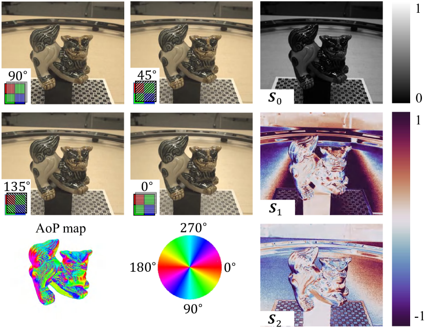
Figure 2: Visualization of polarized images, derived AoP map, and Stokes vectors.

Before dive into the proposed method, we first introduce polarimetric image formation model and derive the photometric cue and geometric cue in our method.

As shown in Fig. 2, a snapshot polarization camera records image observations at four different polarization angles, with its pixel values denoted as $\{I_{0},I_{45},I_{90},I_{135}\}$. This four images reveal the polarization state of received lights, which is represented as a 4D Stokes vector $\mathbf{s}=[s_{0},s_{1},s_{2},s_{3}]$ computed as

$$\begin{dcases}s_{0}=\frac{1}{2}(I_{0}+I_{45}+I_{90}+I_{135})\\ s_{1}=I_{0}-I_{90}\\ s_{2}=I_{45}-I_{135}.\end{dcases}\vspace{-0.5em}$$ (1)

We assume there is no circularly polarized light thus assign $s_{3}$ to be $0$. The Stokes vector can be used to compute the angle of polarization (AoP), i.e.

$$\phi_{a}=\frac{1}{2}\arctan(\frac{s_{2}}{s_{1}}).$$ (2)

Based on the AoP and Stokes vector, we derive the geometric and photometric cue correspondingly.

3.1 Geometric cue

Given AoP $\phi_{a}$, the azimuth angle of the surface can be either $\phi_{a}+\pi/2$ or $\phi_{a}+\pi$, known as the $\pi$ and $\pi/2$ ambiguity depending on whether the surface is specular or diffuse dominant. In this section, we first introduce the geometric cue brought by multiview azimuth map, and then extend it to the case of AoP.

Following MVAS [6], for a scene point $\mathbf{x}$, its surface normal $\mathbf{n}$ and the projected azimuth angle $\phi$ in one camera view follow the relationship as

$$\mathbf{r}_{1}^{\top}\mathbf{n}\cos\phi-\mathbf{r}_{2}^{\top}\mathbf{n}\sin\phi=0,$$ (3)

where $\mathbf{R}=[\mathbf{r}_{1},\mathbf{r}_{2},\mathbf{r}_{3}]^{\top}$ is the rotation matrix of the camera pose. We can further re-arrange Eq. (3) to get the orthogonal relationship between surface normal and a projected tangent vector $\mathbf{t}(\phi)$ as defined below,

$$\mathbf{n}^{\top}\underbrace{(\cos\phi\mathbf{r}_{1}-\sin\phi\mathbf{r}_{2})}_{\mathbf{t}(\phi)}=0.$$ (4)

The $\pi$ ambiguity between AoP and azimuth angle can be naturally resolved as Eq. (4) stands if we add $\phi$ by $\pi$. The $\pi/2$ ambiguity can be addressed by using a pseudo projected tangent vector $\hat{\mathbf{t}}(\phi)$ such that

$$\mathbf{n}^{\top}\underbrace{(\sin\phi\mathbf{r}_{1}+\cos\phi\mathbf{r}_{2})}_{\hat{\mathbf{t}}(\phi)}=0.$$ (5)

If one scene point $\mathbf{x}$ is observed by $f$ views, we can stack Eq. (4) and Eq. (5) based on $k$ different rotations and observed AoPs, leading to a linear system

$$\mathbf{T}(\mathbf{x})\mathbf{n}(\mathbf{x})=\mathbf{0}.$$ (6)

We treat this linear system as our geometric cue for multiview polarized 3D reconstruction.

3.2 Photometric cue

Assuming the incident environment illumination is unpolarized, the Stokes vector of the incident light direction $\bm{\omega}$ can be represented as

$$\mathbf{s}_{i}(\bm{\omega})=L(\bm{\omega})[1,0,0,0]^{\top},$$ (7)

where $L(\bm{\omega})$ denotes the light intensity. The outgoing light recorded by the polarization camera becomes partially polarized due to the reflection. This process is modeled via a $4\times 4$ Muller matrix $\mathbf{H}$. Under an environment illumination, the outgoing Stokes vector $\mathbf{s}_{o}$ can be formulated as the integral of incident Stokes vector multiplicated with the Muller matrix, i.e.

$$\mathbf{s}_{o}(\mathbf{v})=\int_{\Omega}\mathbf{H}\mathbf{s}_{i}(\bm{\omega})\,\,d\bm{\omega},$$ (8)

where $\mathbf{v}$ and $\Omega$ denote the view direction and integral domain. Following the polarized BRDF (pBRDF) model [2], the output Stokes vector can be decomposed into the diffuse and specular parts modeled via $\mathbf{H}_{d}$ and $\mathbf{H}_{s}$ correspondingly, i.e.

$$\mathbf{s}_{o}(\mathbf{v})=\int_{\Omega}\mathbf{H}_{d}\mathbf{s}_{i}(\bm{\omega})\,\,d\bm{\omega}+\int_{\Omega}\mathbf{H}_{s}\mathbf{s}_{i}(\bm{\omega})\,\,d\bm{\omega}.$$ (9)

Following the derivation from PANDORA [9], we can furhter formulate the output Stokes vector as

$$\mathbf{s}_{o}(\mathbf{v})=L_{d}\begin{bmatrix}T_{o}^{+}\\ T_{o}^{-}\cos(2\phi_{n})\\ -T_{o}^{-}\sin(2\phi_{n})\\ 0\end{bmatrix}+L_{s}\begin{bmatrix}R^{+}\\ R^{-}\cos(2\phi_{h})\\ -R^{-}\sin(2\phi_{h})\\ 0\end{bmatrix},$$ (10)

where $L_{d}=\int_{\Omega}\rho L(\bm{\omega})\bm{\omega}^{\top}\mathbf{n}\,T_{i}^{+}T_{i}^{-}\,d\bm{\omega}$ is denoted as diffuse radiance related to surface normal $\mathbf{n}$, Fresnel transmission coefficients [2] $T_{i,o}^{+}$ and $T_{i,o}^{-}$, diffuse albedo $\rho$, and the azimuth angle of incident light $\phi_{n}$. $L_{s}=\int_{\Omega}L(\bm{\omega})\frac{DG}{4\mathbf{n}^{\top}\mathbf{v}}\,\,d\bm{\omega}$ denotes specular radiance related to Fresnel reflection coefficients [2] $R^{+}$ and $R^{-}$, the incident azimuth angle $\phi_{h}$ w.r.t. the half vector $\mathbf{h}=\frac{\bm{\omega}+\mathbf{v}}{\|\bm{\omega}+\mathbf{v}\|_{2}^{2}}$, and the normal distribution and shadowing term $D$ and $G$ in the Microfacet model [31]. Please check supplementary material for more details.

Based on polarimetric image formation model shown in Eq. (10), we build the photometric cue.

4 Proposed method

Our NeRSP takes sparse multiview polarized images, the corresponding silhouette mask of the target object, and camera poses as input, outputs surface shape of the object represented implicitly via SDF. We begin by the discussion on photometric cue and geometric cue in resolving the shape reconstruction ambiguity, followed by the instruction of network structure and loss function of our NeRSP.

4.1 Ambiguity in sparse 3D reconstruction

The geometric cue and photometric cue play an important role in reducing the solution space of the surface shape under sparse views. As shown in Fig. 3, we illustrate the shape estimation under 2 views with different cues. Given only RGB images as input (corresponding to the setting in NeRO [19] and S-VolSDF [35]), different combination of scene point positions, surface normals, and reflectance properties such as albedo can lead to the same image observations, since there are only two RGB measurements for each 3D points along the camera ray. With Stokes vectors extracted from the polarized images, the photometric cue brings $6$ measurements for each 3D points (Stokes vector has $3$ elements), reducing the surface normal candidates unfit to the polarimetric image formation model.

On the other hand, based on AoP maps from polarized images, we can uniquely determine the surface normal up to a $\pi$ ambiguity for every scene point along the camera ray. However, it is still ambiguous to find the position where camera ray intersects the surface, unless the third view is provided [6]. Therefore, under sparse views setting (e.g., 2 views in Fig. 3), determining scene point position based on either geometric or photometric cue remains ambiguous.

Our method combines these two cues derived from polarized images. As visualized in the bottom-right part of Fig. 3, the correct scene point position should have its surface normal lay in the intersection of normal candidate groups derived from both photometric and geometric cues. As surface normal at different sampled scene point is uniquely determined by geometric cue, we can easily determine whether the point is on the surface with the aid of photometric cue. In this way, we reduce the solution space of sparse-shot reflective surface reconstruction.

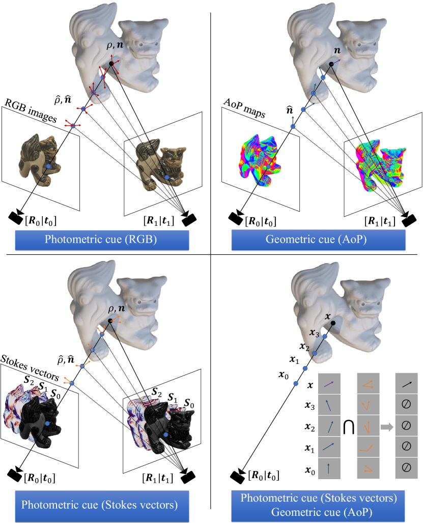
Figure 3: Ambiguity of determining 3D postions under sparse views with geometric and photometric cues.

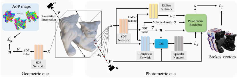
Figure 4: Pipeline of our NeRSP.

4.2 NeRSP

Network structure

As shown in Fig. 4, our NeRSP applies a similar network structure with PANDORA [9] originally derived from Ref-NeRF [30]. For a light ray emitted from camera center $\mathbf{o}$ with the direction $\mathbf{v}$, we sample a point on the ray with travel distance $t_{i}$, its location is denoted at $\mathbf{x}_{i}=\mathbf{o}+t_{i}\mathbf{v}$. Following the volume rendering used in NeRF [25], the observed Stokes vector $\mathbf{s}(\mathbf{v})$ can be integrated by the volume opacity $\sigma_{i}$ and the Stokes vectors at the sampled points along the ray, i.e.

$$\mathbf{s}(\mathbf{v})=\sum_{i=1}^{n}W_{i}\mathbf{s}_{o}(\mathbf{x}_{i},\mathbf{v})\sigma_{i},$$ (11)

where $W_{i}=\prod_{j=1}^{i-1}(1-\sigma_{j})$ denote the accumulated transmittance of a sampled point.

Motivated by recent neural 3D reconstruction method NeuS [33], we derives the volume opacity from a SDF network and also extract the surface normal from the gradient of the SDF. To compute $\mathbf{s}_{o}(\mathbf{x}_{i},\mathbf{v})$ at sampled points, we follows the polarmetric image formation model in Eq. (10). Specifically, the diffuse radiance $L_{d}$ is related to the diffuse albedo and Fresnel transmission coefficients, which depends on the scene positions but invariant to the view direction. Therefore, we use a diffuse radiance network to map $L_{d}$ from the feature of each scene point. The specular radiance $L_{s}$ is related to the specular lobe determined by the view direction, surface normal, and the surface roughness. We therefore use a RoughnessNet to predict surface roughness. Together with the camera view direction and predicted surface normal, we estimate the specular radiance $L_{s}$ following the integrated positional encoding module proposed by Ref-NeRF [30]. Combining $L_{d}$ and $L_{s}$, we reconstruct the observed Stokes vector following Eq. (10).

Loss function

The photometric loss is defined as the L1 distance between the observed $\hat{\mathbf{s}}(\mathbf{v})$ and reconstructed Stokes vectors $\mathbf{s}(\mathbf{v})$, i.e.,

$$\mathcal{L}_{p}=\sum_{\mathbf{v}\in\mathcal{V}}\|\mathbf{s}(\mathbf{v})-\hat{\mathbf{s}}(\mathbf{v})\|_{1},$$ (12)

where $\mathcal{V}$ denotes all the camera rays casted within object masks at different views.

For the geometric loss. we first find the 3D scene point $\mathbf{x}$ along the camera ray $\mathbf{v}$ until touching the surface and then locate the projected 2D pixel positions at different views. The geometric loss is defined based on the Eq. (6), i.e.,

$$\mathcal{L}_{g}=\sum_{\mathbf{x}\in\mathcal{X}}\|\mathbf{T}(\mathbf{x})\mathbf{n}(\mathbf{x})\|_{2}^{2},$$ (13)

where $\mathcal{X}$ denotes all the ray-surface intersections inside the object masks at different views.

Besides the photometric and geometric loss, we add mask loss supervised by the object masks and the Eikonal regularization loss. The mask loss is defined as

$$\mathcal{L}_{m}=\sum{\rm BCE}({M}_{k},{O}_{k}),$$ (14)

where $O_{k}=\sum_{i=1}^{n}W_{k,i}\sigma_{k,i}$ represents the predicted mask at $k$-th camera ray, whose GT mask value is denoted as $M_{k}$. BCE represents binary cross entropy loss.

The Eikonal loss is defined as

$$\mathcal{L}_{e}=\frac{1}{nf}\sum_{i,k}(\|\mathbf{n}_{i,k}\|-1)^{2},$$ (15)

where $\mathbf{n}_{i,k}$ is the surface normal derived from the SDF network at $i$-th sampled point along $k$-th camera ray.

Our NeRSP is supervised by the combination of the above loss terms, i.e.

$$\mathcal{L}=\mathcal{L}_{p}+\lambda_{g}\mathcal{L}_{g}+\lambda_{m}\mathcal{L}_{m}+\lambda_{e}\mathcal{L}_{e},$$ (16)

where $\lambda_{e},\lambda_{m}$ and $\lambda_{p}$ are the coefficients for the corresponding loss terms.

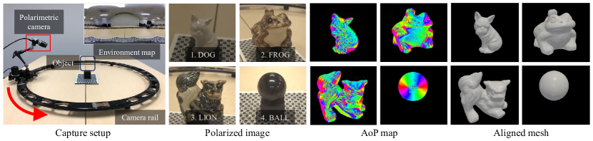
Figure 5: Capture setup and overview of our real-world multiview polarized image dataset RMVP3D.

4.3 RMVP3D Dataset

To quantitatively evaluate the proposed method, we capture a Real-world Multiview Polarized image dataset with aligned ground truth meshes. Figure 5 (left) illustrates our capturing setup, which includes a polarimetric camera, FLIR BFS-U3-51S5PC-C, equipped with a $12$ mm lens and a rotation rail. We use OpenCV for demosaicing the raw data and obtain $1224\times 1024$ color images with polarizer angles at $0$, $45$, $90$, and $135$ degrees. During the data capture, we place target objects at the center of the rail, and capture 60 images per object by manually moving the camera. We collect $4$ objects as targets: Dog, Frog, Lion, and Ball, as shown in Fig. 5 (middle). For the quantitative evaluation, we adopt a laser scanner Creaform HandySCAN BLACK with the accuracy of $0.01$ mm to obtain the ground truth mesh. To align the mesh to the captured image views, we first apply PANDORA [9] to estimated a reference shape using all available views and then align the scanned mesh to the estimated one via ICP algorithm [4]. Besides the ground-truth shapes and multiview images, we also capture the environment map using a 360-degree camera THETA Z1, benefiting quantitative evaluations on the illumination estimation for related neural inverse rendering works.

5 Experiments

We evaluate NeRSP with three experiments: 1) comparison with existing multiview 3D reconstruction methods quantitatively on synthetic dataset; 2) ablation study on the contribution of geometric and photometric loss terms 3) qualitative and quantitative evaluations on real-world datasets. We also provide the BRDF and novel view results in the supplementary material.

Hedgehog	Squirrel	Snail	David	Dragon

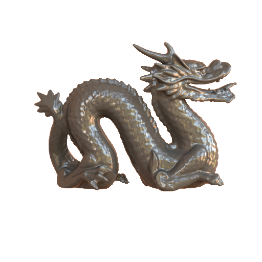
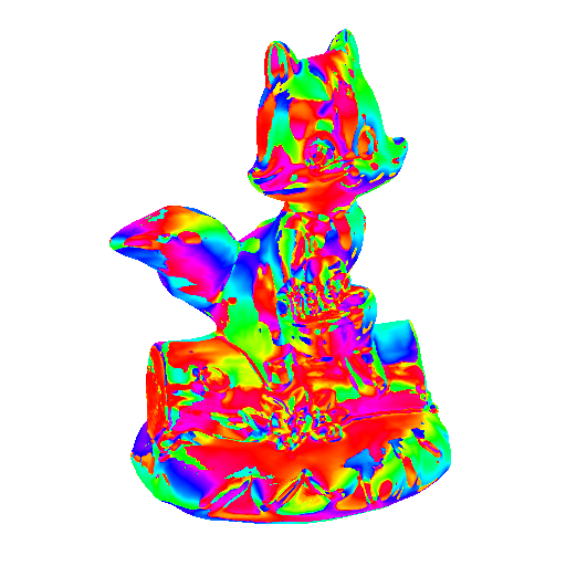
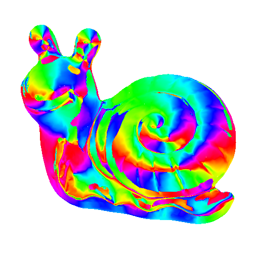
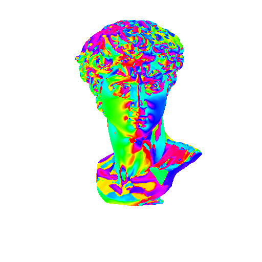
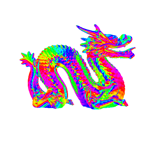
Figure 6: Overview of synthetic dataset SMVP3D. Top and bottom rows show image observations and the corresponding AoP maps.

5.1 Datasets & Baselines

Dataset.

We prepare two real-world datasets: the PANDORA dataset [9] and our proposed RMVP3D, where PANDORA dataset [9] is only used for qualitative evaluation as the ground truth meshes are not provided. We also prepare a synthetic multiview polarized image dataset SMVP3D with Mitsuba rendering engine [15], which contains $5$ objects with spatially-varying and reflective reflectance, as visualized in Fig. 6. The objects are illuminated by environment maps and captured by $6$ views randomly distributed around the objects. Besides rendered polarized images, we also export the stokes vectors, GT surface normal maps, and AoP maps for each object.

Baselines.

Our work solves multiview 3D reconstruction for reflective surfaces based on sparse polarized images. Therefore, we choose the state-of-the-art 3D reconstruction methods targeting reflective surfaces NeRO [19] and sparse views S-VolSDF [35]. The above two methods are based on RGB image inputs. For multiview stereo based on polarized images, we select PANDORA [9] and MVAS [6] as our baselines. NeRO [19] does not require silhouette masks as input. For a fair comparison, we remove the background in the RGB images with the corresponding masks before inputting to NeRO [19]. To compare different methods, we apply Chamfer distance (CD) between the estimated and the GT meshes, and the mean angular error (MAE) between the estimated and the GT surface normals at different views as our evaluation metrics.

5.2 Shape recovery on synthetic dataset

As shown in Table 1, we summarize the shape estimation error of existing methods and ours on SMVP3D. Our method achieves the smallest Chamfer distance along all of the $5$ synthetic objects. Based on the visualized shape estimates shown in Fig. 7, NeRO [19] and S-VolSDF [35] cannot accurately recover surface details as highlighted in the closed-up views. One possible reason is that the disentanglement of the shape and reflective reflectance from the sparse images is too challenging for these methods based on only RGB information. MVAS [6] and PANDORA [9] address the geometric and photometric cues of the polarized images, separately. However, the reconstructed reflective surface shapes are still unsatisfactory due to the ambiguities in geometric and photometric cues under the sparse views setting. As highlighted in the closed-up views, benefiting from both geometric and photometric cues, our method reduces the solution space of shape estimation, leading to the most reasonable shape recoveries compared with the GT shapes.

Table 1: Comparison on shape recoveries on synthetic dataset evaluated by Chamfer distance ($\downarrow$). The smallest and second smallest errors are labeled in bold and underlined. “N/A” denotes the experiment where a specific method cannot output reasonable shape estimation results.

Method	Hedgehog	Squirrel	Snail	David	Dragon
NeRO [19]	5.39	4.69	14.19	45.8	6.51
S-VolSDF [35]	7.33	5.33	16.8	$\underline{5.12}$	N/A
MVAS [6]	$\underline{5.37}$	5.72	$\underline{8.01}$	7.01	$\underline{6.48}$
PANDORA [9]	9.33	11.1	18.8	7.86	17.4
NeRSP (Ours)	3.43	4.55	5.59	4.16	4.77

GT	NeRO [19]	S-VolSDF [35]
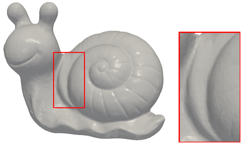
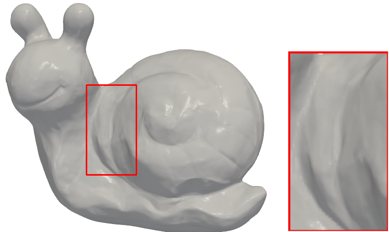
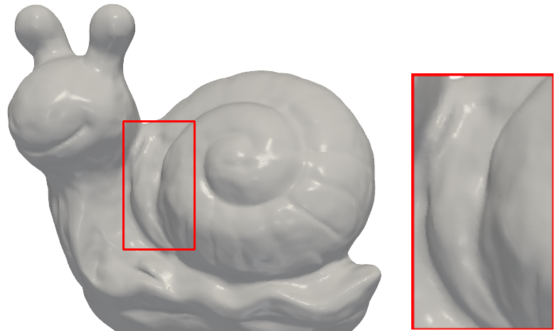
MVAS [6]	PANDORA [9]	NeRSP (ours)

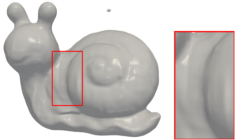
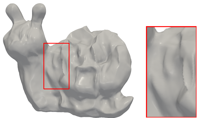
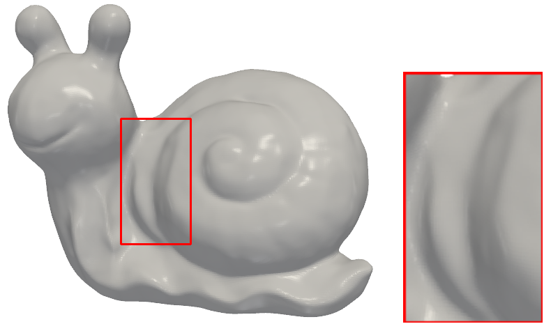
Figure 7: Qualitative evaluation on shape recoveries from $6$ sparse inputs. Our recovered shapes are closer to the GT, as highlighted in the closed-up views.

Besides the evaluation of the reconstructed mesh, we also test the surface normal estimation results. As shown in Table 2, we summarize the mean angular errors of estimated surface normals at $6$ views from different methods. Consistent with the evaluation results in Table 1, NeRSP achieves the smallest mean angular errors in average. We also observed that the results from NeRO [19], MVAS [6], and PANDORA [9] have larger errors on objects with fine details, such as David and Dragon objects. As an example, MVAS [6] has the second smallest Chamfer distance shown in Table 1, but the mean angular error is over $20^{\circ}$. One potential reason is existing methods output smooth shapes in the sparse views setting, where the surface details such as the flakes of the Dragon are not well recovered.

5.3 Ablation study

In this section, we conduct an ablation study to test the effectiveness of geometric and photometric cues. Taking the Dragon object as an example, we conduct our method with and without the photometric loss ${\mathcal{L}_{p}}$ and the geometric loss ${\mathcal{L}}_{g}$. As shown in Fig. 8, we plot the shape and surface normal estimations by disabling the different loss terms. Without the photometric loss, the shape ambiguity due to the sparse views occurs. As shown from the closed-up views, the shape near the leg part has a concave artifact, as there are only two visible views for this region, unable to formulate a unique solution for the shape merely based on the AoP maps [6]. Without geometric loss, we also obtain distorted shape results as the sparse image observations are not sufficient to uniquely decompose the shape, reflectance, and illumination. By combining the photometric and geometric loss, our NeRSP reduces the ambiguity of shape recovery and the estimated shape is closer to the GT, as highlighted in the closed-up views.

Table 2: Comparison on surface normal estimation on synthetic dataset evaluated by mean angular error (MAE) ($\downarrow$).

Method	Hedgehog	Squirrel	Snail	David	Dragon
NeRO [19]	9.14	10.15	11.45	42.02	24.22
S-VolSDF [35]	11.26	13.28	7.59	17.05	N/A
MVAS [6]	7.06	10.28	6.19	21.86	24.29
PANDORA [9]	19.75	23.52	16.54	21.88	28.82
NeRSP (Ours)	7.89	9.80	4.82	13.70	18.03

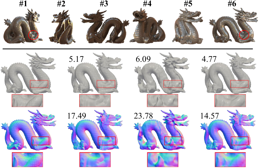
GT   w/o $\mathcal{L}_{p}$     w/o $\mathcal{L}_{g}$       Ours

Figure 8: Ablation study on different loss terms. The top and bottom rows visualize the estimated shape and surface normal, with the Chamfer distance and the mean angular error labeled on the top of each sub-figure, respectively.

5.4 Shape recovery on real data

Besides the synthetic experiments shown in the previous section, we also evaluate our method on real-world datasets PANDORA dataset [9] and RMVP3D to test its applicability in real-world 3D reconstruction scenarios.

Qualitative evaluation on PANDORA dataset [9].

As shown in Fig. 9, we provide qualitative evaluations on PANDORA dataset [9]. Compared to the image appearance with the estimated results from S-VolSDF [35] and NeRO [19], the shape is not fully disentangled from the reflectance, leading to bumpy surface shapes that are closely related to the reflectance texture. MVAS [6] and PANDORA [9] have over-smoothed shape estimates or concave shape artifacts, due to addressing only geometric or photometric cues under the sparse capture setting. Our shape estimation results have no such shape artifacts and match the image observations closely.

Polarized image	NeRO [19]	S-VolSDF [35]	MVAS [6]
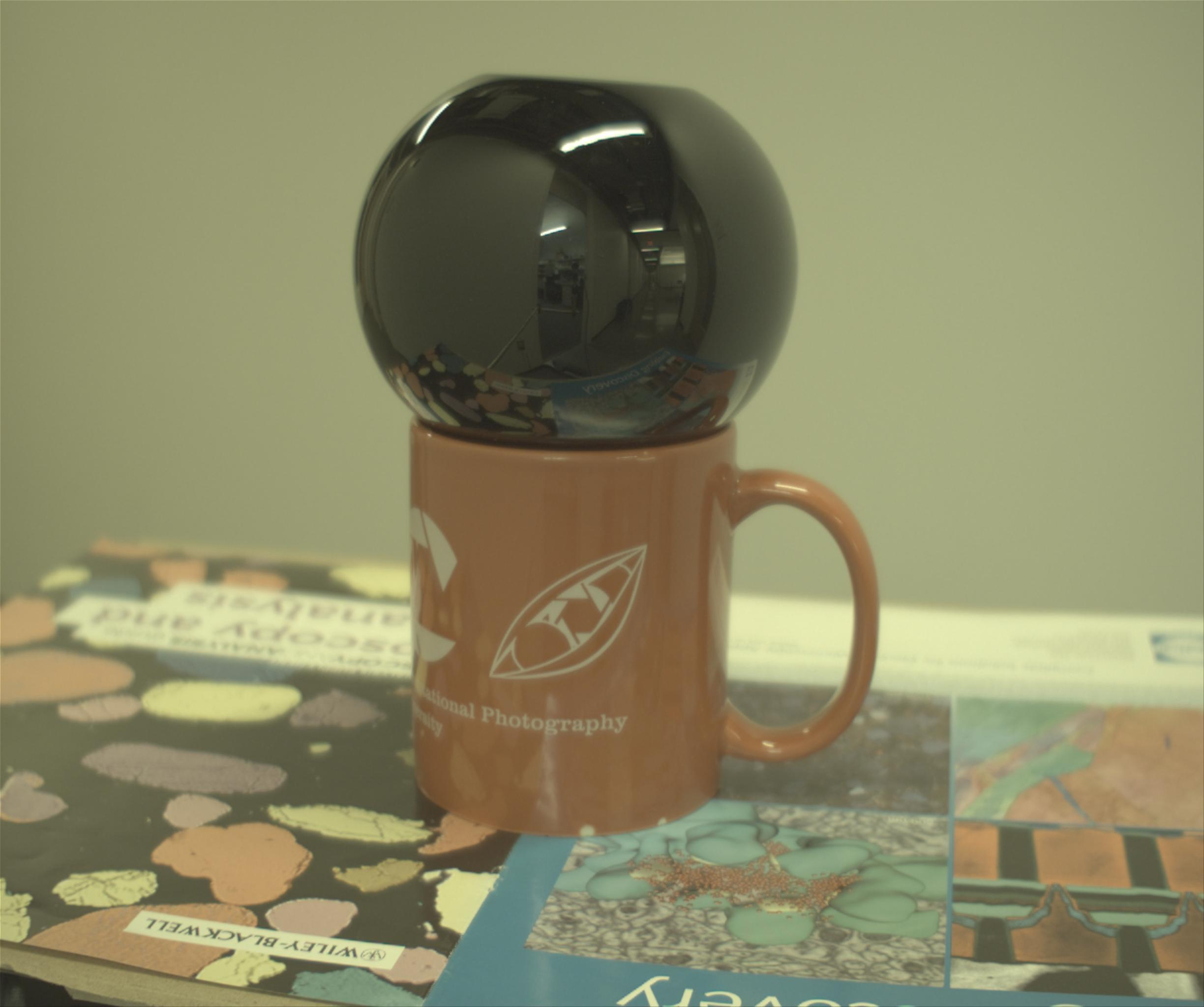
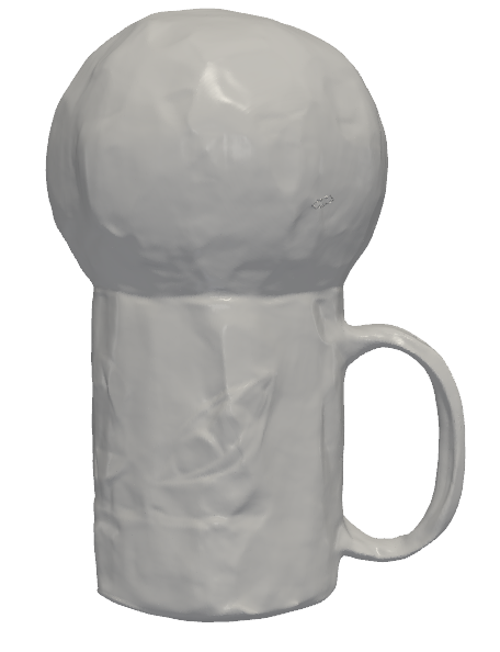
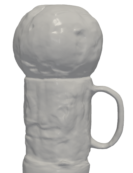
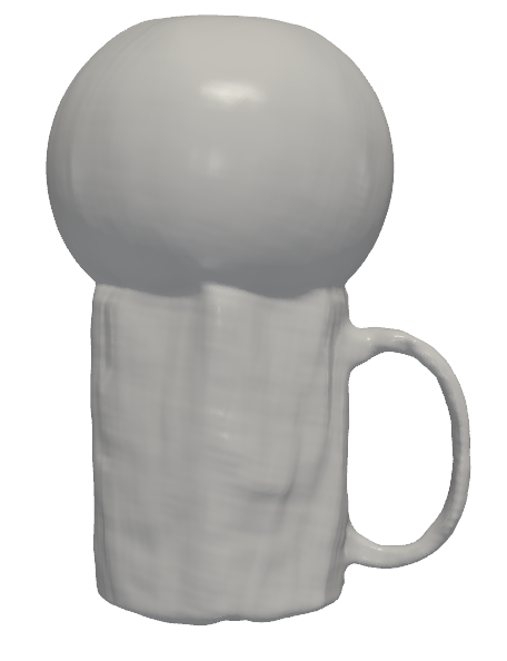
AoP map	PANDORA [9]	NeRSP (Ours)
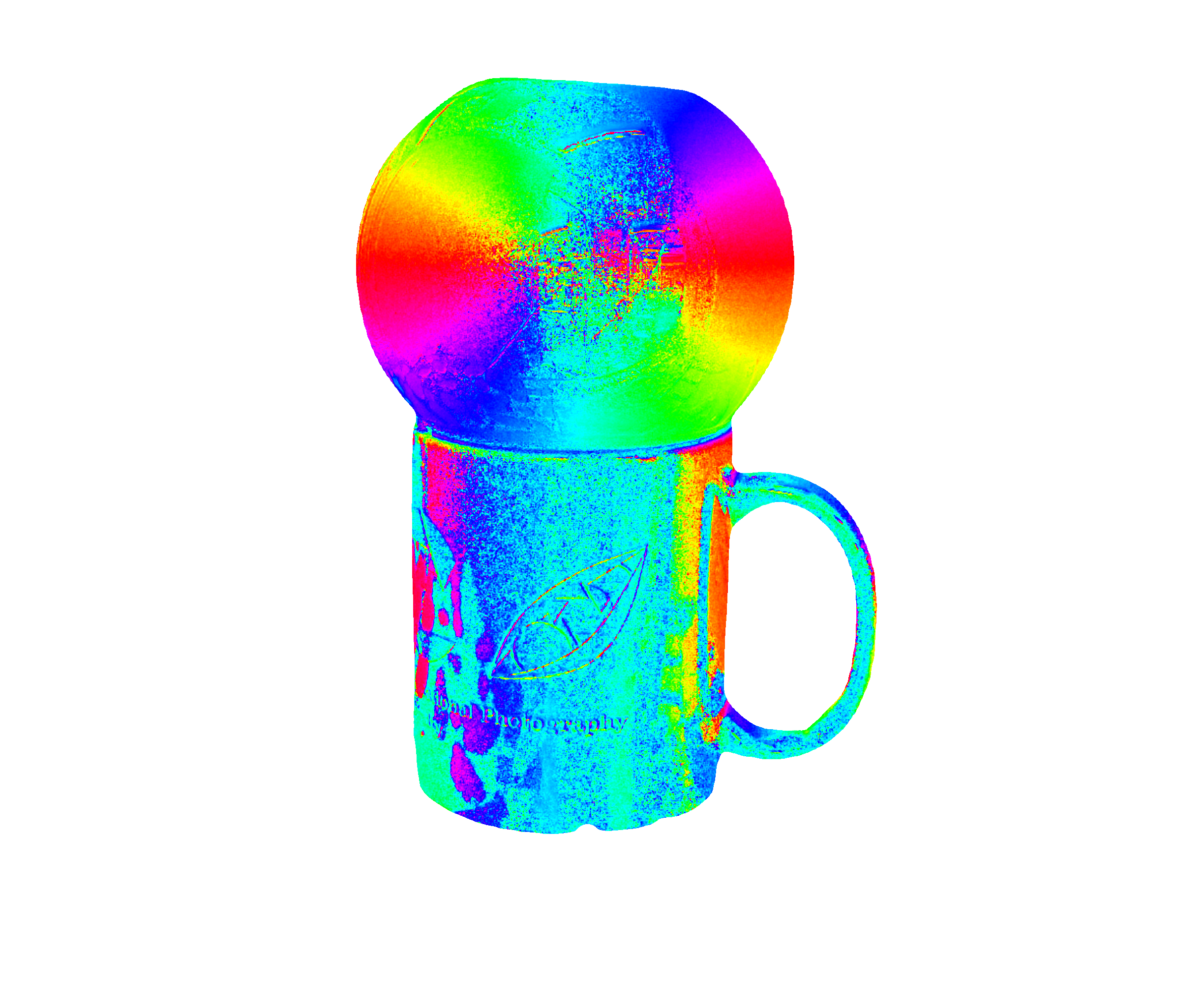
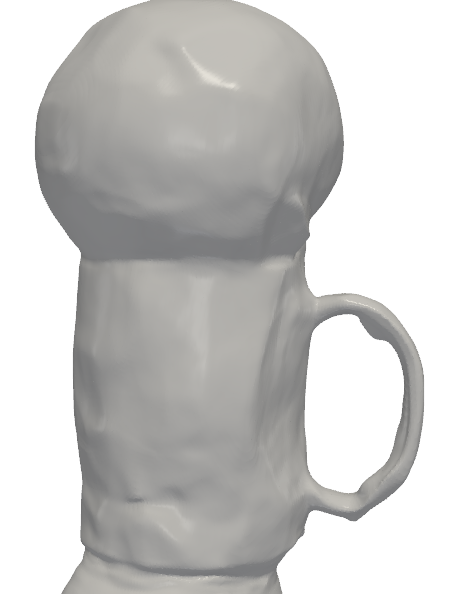
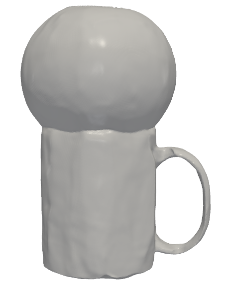
Polarized image	NeRO [19]	S-VolSDF [35]	MVAS [6]
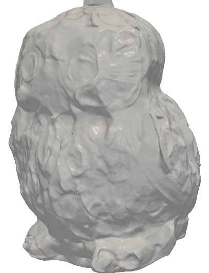
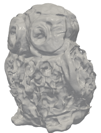
AoP map	PANDORA [9]	NeRSP (Ours)

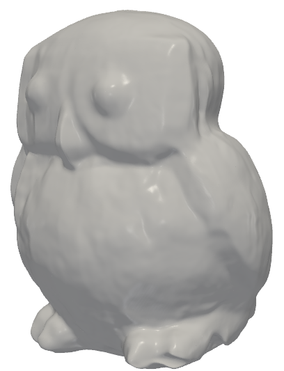
Figure 9: Qualitative evaluation on PANDORA dataset [9].

Table 3: Quantitative evaluation on RMVP3D with Chamfer distance ($\downarrow$). Our method achieves the smallest error on average.

Method	Dog	Lion	Frog	Ball	Average
NeRO [19]	9.11	10.74	6.21	3.87	$\underline{7.48}$
S-VolSDF [35]	9.93	7.39	7.91	18.4	10.91
MVAS [6]	9.23	7.51	9.90	4.77	7.86
PANDORA [9]	14.3	15.04	11.27	3.96	11.14
NeRSP (Ours)	8.80	5.18	6.70	3.84	6.13

Quantitative evaluation on RMVP3D.

As shown in Table 3, we present a quantitative evaluation on RMVP3D based on Chamfer distance. Consistent with the synthetic experiment, our NeRSP achieves the smallest estimation error in average. The visualized shapes shown in Fig. 10 further reveal that reflective surfaces are challenging to S-VolSDF [35] for disentangling the shape from reflectance, as highlighted by the bumpy surface of the Frog object in the closed-up views. NeRO [19] and PANDORA [9] have similar estimation error with us on the simple Ball object. For complex shapes like Lion, distorted shape recoveries are obtained from these methods due to the sparse views setting, while ours are closer to the GT meshes, demonstrating the effectiveness of our method on real-world reflective surface reconstruction under sparse inputs.

GT	NeRO [19]	S-VolSDF [35]
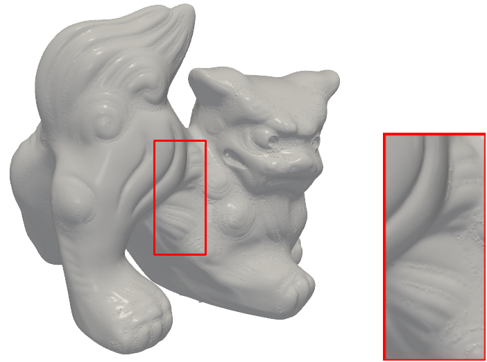
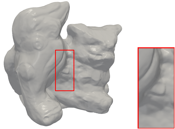
MVAS [6]	PANDORA [9]	NeRSP (ours)
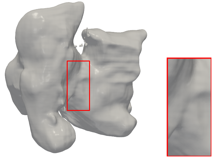
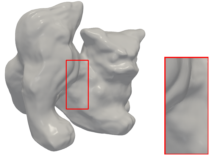
GT	NeRO [19]	S-VolSDF [35]
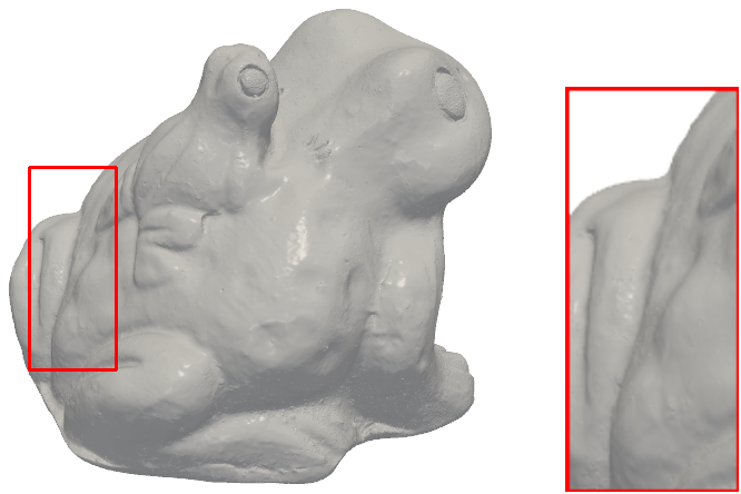
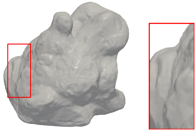
MVAS [6]	PANDORA [9]	NeRSP (ours)

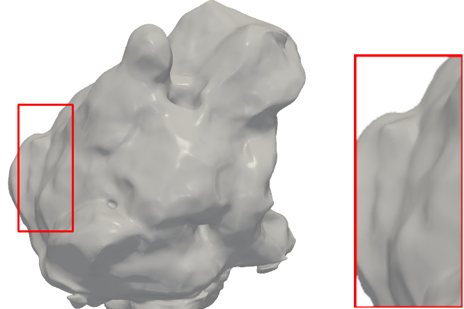
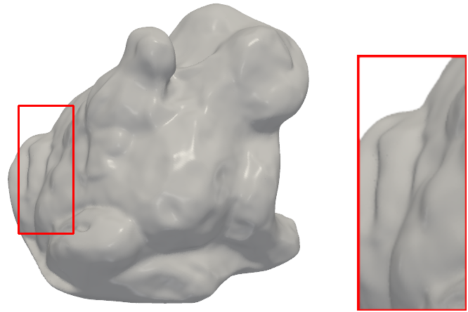
Figure 10: Comparison on shape recoveries on RMVP3D dataset.

6 Conclusion

We propose NeRSP, a neural 3D reconstruction method for reflective surfaces under sparse polarized images. Due to the challenges of shape-radiance ambiguity and complex reflectance, existing methods struggle with either reflective surfaces or sparse views and cannot address both problems with RGB images. We propose to use polarized images as input. By combining the geometric and photometric cues extracted from polarized images, we reduce the solution space of the estimated shape, allowing for the effective recovery of reflective surface with as few as $6$ views, as demonstrated by publicly available and our own datasets.

Limitation

The inter-reflections and polarized environment light are not considered in this work, which could influence the shape reconstruction accuracy. We noticed a most recent work NeISF [17] focusing on this topic, and we are interested in combining our sparse shot merit with this work in the future.

Acknowledgment

This work was supported by the Beijing Natural Science Foundation Project No. Z200002, the National Nature Science Foundation of China (Grant No. 62136001, 62088102, 62225601, U23B2052), the Youth Innovative Research Team of BUPT No. 2023QNTD02, and the JSPS KAKENHI (Grant No. JP22K17910 and JP23H05491). We thank Youwei Lyu for insightful discussions.

References

- Ba et al. [2020] Yunhao Ba, Alex Gilbert, Franklin Wang, Jinfa Yang, Rui Chen, Yiqin Wang, Lei Yan, Boxin Shi, and Achuta Kadambi. Deep shape from polarization. In ECCV, pages 554–571, 2020.
- Baek et al. [2018] Seung-Hwan Baek, Daniel S Jeon, Xin Tong, and Min H Kim. Simultaneous acquisition of polarimetric SVBRDF and normals. ACM TOG, 37(6):268–1, 2018.
- Barron et al. [2021] Jonathan T Barron, Ben Mildenhall, Matthew Tancik, Peter Hedman, Ricardo Martin-Brualla, and Pratul P Srinivasan. Mip-NeRF: A multiscale representation for anti-aliasing neural radiance fields. In ICCV, pages 5855–5864, 2021.
- Besl and McKay [1992] Paul J Besl and Neil D McKay. Method for registration of 3-D shapes. In Sensor fusion IV: control paradigms and data structures, pages 586–606, 1992.
- Boss et al. [2021] Mark Boss, Varun Jampani, Raphael Braun, Ce Liu, Jonathan Barron, and Hendrik Lensch. Neural-PIL: Neural pre-integrated lighting for reflectance decomposition. In NeurIPS, pages 10691–10704, 2021.
- Cao et al. [2023] Xu Cao, Hiroaki Santo, Fumio Okura, and Yasuyuki Matsushita. Multi-View Azimuth Stereo via Tangent Space Consistency. In CVPR, pages 825–834, 2023.
- Chen et al. [2021] Anpei Chen, Zexiang Xu, Fuqiang Zhao, Xiaoshuai Zhang, Fanbo Xiang, Jingyi Yu, and Hao Su. MVSNeRF: Fast generalizable radiance field reconstruction from multi-view stereo. In CVPR, pages 14124–14133, 2021.
- Cui et al. [2017] Zhaopeng Cui, Jinwei Gu, Boxin Shi, Ping Tan, and Jan Kautz. Polarimetric multi-view stereo. In CVPR, pages 1558–1567, 2017.
- Dave et al. [2022] Akshat Dave, Yongyi Zhao, and Ashok Veeraraghavan. Pandora: Polarization-aided neural decomposition of radiance. In ECCV, pages 538–556, 2022.
- Deng et al. [2022] Kangle Deng, Andrew Liu, Jun-Yan Zhu, and Deva Ramanan. Depth-supervised NeRF: Fewer views and faster training for free. In CVPR, pages 12882–12891, 2022.
- Ding et al. [2021] Yuqi Ding, Yu Ji, Mingyuan Zhou, Sing Bing Kang, and Jinwei Ye. Polarimetric helmholtz stereopsis. In ICCV, pages 5037–5046, 2021.
- Fukao et al. [2021] Yoshiki Fukao, Ryo Kawahara, Shohei Nobuhara, and Ko Nishino. Polarimetric normal stereo. In CVPR, pages 682–690, 2021.
- Ge et al. [2023] Wenhang Ge, Tao Hu, Haoyu Zhao, Shu Liu, and Ying-Cong Chen. Ref-NeuS: Ambiguity-Reduced Neural Implicit Surface Learning for Multi-View Reconstruction with Reflection. arXiv preprint arXiv:2303.10840, 2023.
- Hartley and Zisserman [2003] Richard Hartley and Andrew Zisserman. Multiple view geometry in computer vision. Cambridge university press, 2003.
- Jakob [2010] Wenzel Jakob. Mitsuba renderer, 2010.
- Lei et al. [2022] Chenyang Lei, Chenyang Qi, Jiaxin Xie, Na Fan, Vladlen Koltun, and Qifeng Chen. Shape from polarization for complex scenes in the wild. In CVPR, pages 12632–12641, 2022.
- Li et al. [2023a] Chenhao Li, Taishi Ono, Takeshi Uemori, Hajime Mihara, Alexander Gatto, Hajime Nagahara, and Yuseke Moriuchi. NeISF: Neural Incident Stokes Field for Geometry and Material Estimation. arXiv preprint arXiv:2311.13187, 2023a.
- Li et al. [2023b] Zhaoshuo Li, Thomas Müller, Alex Evans, Russell H Taylor, Mathias Unberath, Ming-Yu Liu, and Chen-Hsuan Lin. Neuralangelo: High-Fidelity Neural Surface Reconstruction. In CVPR, pages 8456–8465, 2023b.
- Liu et al. [2023] Yuan Liu, Peng Wang, Cheng Lin, Xiaoxiao Long, Jiepeng Wang, Lingjie Liu, Taku Komura, and Wenping Wang. NeRO: Neural Geometry and BRDF Reconstruction of Reflective Objects from Multiview Images. arXiv preprint arXiv:2305.17398, 2023.
- Long et al. [2022] Xiaoxiao Long, Cheng Lin, Peng Wang, Taku Komura, and Wenping Wang. SparseNeuS: Fast generalizable neural surface reconstruction from sparse views. In ECCV, pages 210–227, 2022.
- Lyu et al. [2023] Youwei Lyu, Lingran Zhao, Si Li, and Boxin Shi. Shape from polarization with distant lighting estimation. IEEE TPAMI, 2023.
- Mildenhall et al. [2020] Ben Mildenhall, Pratul P Srinivasan, Matthew Tancik, Jonathan T Barron, Ravi Ramamoorthi, and Ren Ng. NeRF: Representing scenes as neural radiance fields for view synthesis. In ECCV, pages 405–421, 2020.
- Miyazaki et al. [2003] Miyazaki, Tan, Hara, and Ikeuchi. Polarization-based inverse rendering from a single view. In ICCV, pages 982–987, 2003.
- Niemeyer et al. [2020] Michael Niemeyer, Lars Mescheder, Michael Oechsle, and Andreas Geiger. Differentiable volumetric rendering: Learning implicit 3D representations without 3D supervision. In CVPR, pages 3504–3515, 2020.
- Niemeyer et al. [2022] Michael Niemeyer, Jonathan T Barron, Ben Mildenhall, Mehdi SM Sajjadi, Andreas Geiger, and Noha Radwan. Regnerf: Regularizing neural radiance fields for view synthesis from sparse inputs. In CVPR, pages 5480–5490, 2022.
- Oechsle et al. [2021] Michael Oechsle, Songyou Peng, and Andreas Geiger. UNISURF: Unifying neural implicit surfaces and radiance fields for multi-view reconstruction. In ICCV, pages 5589–5599, 2021.
- Park et al. [2019] Jeong Joon Park, Peter Florence, Julian Straub, Richard Newcombe, and Steven Lovegrove. DeepSDF: Learning continuous signed distance functions for shape representation. In CVPR, pages 165–174, 2019.
- Sitzmann et al. [2020] Vincent Sitzmann, Julien Martel, Alexander Bergman, David Lindell, and Gordon Wetzstein. Implicit neural representations with periodic activation functions. In NeurIPS, 2020.
- Smith et al. [2018] William AP Smith, Ravi Ramamoorthi, and Silvia Tozza. Height-from-polarisation with unknown lighting or albedo. IEEE TPAMI, 41(12):2875–2888, 2018.
- Verbin et al. [2022] Dor Verbin, Peter Hedman, Ben Mildenhall, Todd Zickler, Jonathan T Barron, and Pratul P Srinivasan. Ref-NeRF: Structured view-dependent appearance for neural radiance fields. In CVPR, pages 5481–5490, 2022.
- Walter et al. [2007] Bruce Walter, Stephen R Marschner, Hongsong Li, and Kenneth E Torrance. Microfacet models for refraction through rough surfaces. In Proceedings of the 18th Eurographics conference on Rendering Techniques, pages 195–206, 2007.
- Wang et al. [2023] Guangcong Wang, Zhaoxi Chen, Chen Change Loy, and Ziwei Liu. SparseNeRF: Distilling depth ranking for few-shot novel view synthesis. arXiv preprint arXiv:2303.16196, 2023.
- Wang et al. [2021] Peng Wang, Lingjie Liu, Yuan Liu, Christian Theobalt, Taku Komura, and Wenping Wang. NeuS: Learning Neural Implicit Surfaces by Volume Rendering for Multi-view Reconstruction. arXiv preprint arXiv:2106.10689, 2021.
- Wang et al. [2022] Yiqun Wang, Ivan Skorokhodov, and Peter Wonka. HF-NeuS: Improved surface reconstruction using high-frequency details. In NeurIPS, pages 1966–1978, 2022.
- Wu et al. [2023] Haoyu Wu, Alexandros Graikos, and Dimitris Samaras. S-VolSDF: Sparse Multi-View Stereo Regularization of Neural Implicit Surfaces. arXiv preprint arXiv:2303.17712, 2023.
- Yang et al. [2023] Jiawei Yang, Marco Pavone, and Yue Wang. FreeNeRF: Improving Few-shot Neural Rendering with Free Frequency Regularization. In CVPR, pages 8254–8263, 2023.
- Yariv et al. [2020] Lior Yariv, Yoni Kasten, Dror Moran, Meirav Galun, Matan Atzmon, Basri Ronen, and Yaron Lipman. Multiview neural surface reconstruction by disentangling geometry and appearance. In NeurIPS, pages 2492–2502, 2020.
- Yariv et al. [2021] Lior Yariv, Jiatao Gu, Yoni Kasten, and Yaron Lipman. Volume rendering of neural implicit surfaces. In NeurIPS, pages 4805–4815, 2021.
- Yu et al. [2021] Alex Yu, Vickie Ye, Matthew Tancik, and Angjoo Kanazawa. pixelNeRF: Neural radiance fields from one or few images. In CVPR, pages 4578–4587, 2021.
- Zhang et al. [2020] Kai Zhang, Gernot Riegler, Noah Snavely, and Vladlen Koltun. NeRF++: Analyzing and improving neural radiance fields. arXiv preprint arXiv:2010.07492, 2020.
- Zhang et al. [2021a] Kai Zhang, Fujun Luan, Qianqian Wang, Kavita Bala, and Noah Snavely. PhySG: Inverse rendering with spherical gaussians for physics-based material editing and relighting. In CVPR, pages 5453–5462, 2021a.
- Zhang et al. [2021b] Xiuming Zhang, Pratul P Srinivasan, Boyang Deng, Paul Debevec, William T Freeman, and Jonathan T Barron. NeRFactor: Neural factorization of shape and reflectance under an unknown illumination. ACM TOG, 40(6):1–18, 2021b.
- Zhao et al. [2022] Jinyu Zhao, Yusuke Monno, and Masatoshi Okutomi. Polarimetric multi-view inverse rendering. IEEE TPAMI, 2022.