Agnostic Sharpness-Aware Minimization

Abstract

Sharpness-aware minimization (SAM) has been instrumental in improving deep neural network training by minimizing both the training loss and the sharpness of the loss landscape, leading the model into flatter minima that are associated with better generalization properties. In another aspect, Model-Agnostic Meta-Learning (MAML) is a framework designed to improve the adaptability of models. MAML optimizes a set of meta-models that are specifically tailored for quick adaptation to multiple tasks with minimal fine-tuning steps and can generalize well with limited data. In this work, we explore the connection between SAM and MAML, particularly in terms of enhancing model generalization. We introduce Agnostic-SAM, a novel approach that combines the principles of both SAM and MAML. Agnostic-SAM adapts the core idea of SAM by optimizing the model towards wider local minima using training data, while concurrently maintaining low loss values on validation data. By doing so, it seeks flatter minima that are not only robust to small perturbations but also less vulnerable to data distributional shift problems. Our experimental results demonstrate that Agnostic-SAM significantly improves generalization over baselines across a range of datasets and under challenging conditions such as noisy labels and data limitation.

1 Introduction

Deep neural networks have become the preferred method for analyzing data, surpassing traditional machine learning models in complex tasks like classification. These networks process input through numerous parameters and operations to predict classes. Learning involves finding parameters within a model space that minimize errors or maximize performance for a given task. Typically, training data, denoted as $S$, is finite and drawn from an unknown true data distribution $\mathcal{D}$. Larger or more aligned training sets lead to more efficient models.

Despite their ability to learn complex patterns, deep learning models can also capture noise or random fluctuations in training data, leading to overfitting. This results in excellent performance on training data but poor predictions on new, unseen data, especially with domain shifts. Generalization, measured by comparing prediction errors on $S$ and $\mathcal{D}$, becomes crucial. Balancing a model’s ability to fit training data with its risk of overfitting is a key challenge in machine learning.

Several studies have been done on this problem, both theoretically and practically. Statistical learning theory has proposed a number of different complexity measures [37] [7] [27, 8, 32] that are capable of controlling generalization errors. In general, they develop a bound for general error on $\mathcal{D}$. Theory suggests that minimizing the intractable general error on $\mathcal{D}$ is equivalent to minimizing the empirical loss on $S$ with some constraints to the complexity of models and training size [3].

An alternative strategy for mitigating generalization errors involves the utilization of an optimizer to learn optimal parameters for models with a specific local geometry. This approach enables models to locate wider local minima, known as flat minima, which makes them more robust against data shift between train and test sets [20, 30, 13]. The connection between a model’s generalization and the width of minima has been investigated theoretically and empirically in many studies, notably [18, 28, 12, 17]. A specific method within this paradigm is Sharpness-aware Minimisation (SAM) [16], which has emerged as an effective technique for enhancing the generalization ability of deep learning models. SAM seeks a perturbed model within the vicinity of a current model that maximizes the loss over a training set. Eventually, SAM leads the model to the region where both the current model and its perturbation model have low loss values, which ensure flatness. The success of SAM and its variants [24, 23, 36] has inspired further investigation into its formulation and behavior, as evidenced by recent works such as [21, 26, 5].

SAM significantly enhances robustness against shifts between training and test datasets, thereby reducing overfitting and improving overall performance across different datasets and domains. This robust optimization approach aligns particularly well with the principles of Model-Agnostic Meta-Learning (MAML) [14]. MAML aims to find a set of meta-model parameters that not only generalize well on current tasks but can also be quickly adapted to a wide range of new tasks. Furthermore, the agnostic perspective of MAML is particularly enticing for enhancing generalization ability because it endeavors to learn the optimal meta-model from meta-training sets capable of achieving minimal losses on independent meta-testing sets, thus harmonizing with the goal of generalization.

In this paper, inspired by MAML, we initially approach the problem of learning the best model over a training set from an agnostic viewpoint. Subsequently, we harness this perspective with sharpness-aware minimization to formulate an agnostic optimization problem. Additionally, a naive solution akin to MAML does not suit our objectives. Hence, we propose a novel solution for this agnostic optimization problem, resulting in an approach called AgnosticSAM. In summary, our contributions in this work are as follows:

• We proposed a framework inspired by SAM and MAML works, called Agnostic-SAM to improve model flatness and robustness against noise. Agnostic-SAM update model to a region that minimizes the sharpness of the model on the training set while also implicitly performing well on the validation set by using a combination of gradients on both training and validation sets.

• We examine standard image classification tasks across multiple datasets and models to demonstrate the effectiveness of Agnostic-SAM in enhancing generalization error compared to baseline methods. Additionally, we assess our approach under noisy label conditions with varying levels of noise. The consistent improvement in performance is evidence that Agnostic-SAM not only enhances robustness against label noise but also contributes to more stable and reliable predictions across different settings.

2 Related works

Sharpness-Aware Minimization.

The correlation between the wider minima and the generalization capacity has been extensively explored both theoretically and empirically in various studies [20, 30, 13]. Many works suggested that finding flat minimizers might help to reduce generlization error and increase robustness to data distributional shift problems in various settings [20, 30, 13]. There are multiple works have explored the impact of different training parameters, including batch size, learning rate, gradient covariance, and dropout, on the flatness of discovered minima such as [22, 19, 39].

Sharpness-aware minimization (SAM) [16] is a recent optimization technique designed to improve the generalization error of neural networks by considering the sharpness of the loss landscape during training. SAM minimizes the worst-case loss around the current model and effectively updates models towards flatter minima to achieve low training loss and maximize generalization performance on new and unseen data. SAM has been successfully applied to various tasks and domains, such as vision models [11], language models [6], federated learning [33], Bayesian Neural Networks [29], domain generalization [9], multi-task learning [31] and meta-learning bi-level optimization [1]. In  [1], authors discussed SAM’s effectiveness in enhancing meta-learning bi-level optimization, while SAM’s superior convergence rates in federated learning compared to existing approaches in  [33] along with proposing a generalization bound for the global model.

Model-Agnostic Machine Learning.

Model-agnostic machine learning techniques have significantly advanced, offering flexible solutions applicable across various models and tasks. Notable methods like LIME [35] and SHAP [25] provide model-agnostic interpretability, allowing users to understand complex models by approximating them with simpler, interpretable models or by attributing predictions to individual features. Additionally, MAML [14] stands out as the most compelling model-agnostic technique that formulates meta-learning as an optimization problem, enabling models to adapt to new tasks with minimal task-specific modifications quickly. Subsequent research has largely focused on addressing the computational challenges of MAML [10, 38] or proposing novel approaches that exploit the concept of model agnostic from MAML across a wide range of tasks, including non-stationary environments [2], alternative optimization strategies [34], and uncertainty estimation for robust adaptation [15].

3 Proposed Framework

3.1 Notions

We start with introducing the notions used throughout our paper. We denote $\mathcal{D}$ as the data/label distribution to generate pairs of data/label $(x,y)$. Given a model with the model parameter $\theta$, we denote the per sample loss induced by $(x,y)$ as $\ell(x,y;\theta)$. Let $S$ be the training set drawn from the distribution $\mathcal{D}$. We denote the empirical and general losses as $\mathcal{L}_{S}\left(\theta\right)=\mathbb{E}_{S}\left[\ell\left(x,y;\theta\right)\right]$ and $\mathcal{L}_{\mathcal{D}}\left(\theta\right)=\mathbb{E}_{\mathcal{D}}\left[\ell\left(x,y;\theta\right)\right]$ respectively. Moreover, we define $\mathcal{L}_{\mathcal{D}}\left(\theta\mid S\right)$ as an upper bound defined over $S$ of the general loss $\mathcal{L}_{\mathcal{D}}\left(\theta\right)$. Finally, we use $|A|$ to denote the cardinality of a set $A$.

3.2 Problem Formulation

Given a training set $S^{t}$ whose examples are sampled from $\mathcal{D}$ (i.e., $S^{t}\sim\mathcal{D}^{N_{t}}$ with $N_{t}=|S^{t}|$), we use $\mathcal{L}_{\mathcal{D}}\left(\theta\mid S^{t}\right)$ to train models and among the models that minimize this loss, we select the one that minimize the general loss as follows:

$$\min_{\theta^{*}}\mathcal{L}_{\mathcal{D}}\left(\theta^{*}\right)\text{ s.t. }\theta^{*}\in\mathcal{A}_{\mathcal{D}}\left(S^{t}\right)=\text{argmin}_{\theta}\mathcal{L}_{\mathcal{D}}\left(\theta\mid S^{t}\right).$$ (1)

The reason for the formulation in (1) is that although $\mathcal{L}_{\mathcal{D}}\left(\theta\mid S_{t}\right)$ is an upper bound of the general loss $\mathcal{L}_{\mathcal{D}}\left(\theta\right)$, there always exists a gap between them. Therefore, the additional outer minimization helps to refine the solutions. We now denote $S^{v}$ (i.e., $S^{v}\sim\mathcal{D}^{N_{v}}$ with $N_{v}=|S^{v}|$) as a valid set sampled from $\mathcal{D}$. With respect to this valid set, we have the following theorem.

Theorem 1.

Denote $\mathcal{L}_{\mathcal{D}}\left(\theta\mid S\right):=\max_{\theta^{\prime}:\|\theta^{\prime}-\theta\|_{2}\leq\rho}\mathcal{L}_{S}\left(\theta^{\prime}\right)$. Under some mild condition similar to SAM [16], with a probability greater than $1-\delta$ (i.e., $\delta\in[0,1]$) over the choice of $S^{v}\sim\mathcal{D}^{N_{v}}$, we then have for any optimal models $\theta^{*}\in\mathcal{A}_{\mathcal{D}}(S^{t})$:

$$\mathcal{L}_{\mathcal{D}}\left(\theta^{*}\right)\leq\mathcal{L}_{\mathcal{D}}\left(\theta^{*}\mid S^{v}\right)+\frac{4L}{\sqrt{N_{v}}}\left[k\log\left(1+\frac{\|\theta^{*}\|^{2}}{\rho}\left(1+\sqrt{\log N_{v}/k}\right)\right)+2\sqrt{\log\frac{N_{v}+k}{\delta}}+O(1)\right],$$ (2)

where $L$ is the upper-bound of the loss function (i.e., $\ell\left(x,y;\theta\right)\leq L,\forall x,y,\theta$), $k$ is the model size, and $\rho>0$ is the perturbation radius.

Our theorem 1 (proof can be found in Appendix A.1) can be viewed as an extension of Theorem 1 in [16], where we apply the Bayes-PAC theorem from [4] to prove an upper bound for the general loss of any bounded loss, instead of the 0-1 loss in [16]. Moreover, we can generalize this proof for $S^{t}$ to explain why using $\mathcal{L}_{\mathcal{D}}\left(\theta\mid S^{t}\right):=\max_{\theta^{\prime}:\|\theta^{\prime}-\theta\|_{2}\leq\rho}\mathcal{L}_{S^{t}}\left(\theta^{\prime}\right)$ as an objective to minimize, as in (1). Thanks to Theorem 1, we can rewrite the objectives in (1) as:

$$\min_{\theta^{*}}\mathcal{L}_{\mathcal{D}}\left(\theta^{*}\mid S^{v}\right)\text{ s.t. $\theta^{*}$$\in\mathcal{A}_{\mathcal{D}}\left(S^{t}\right)=\text{argmin}_{\theta}\,\mathcal{L}_{\mathcal{D}}$$\left(\theta\mid S^{t}\right)$},$$ (3)

where $\mathcal{L}_{\mathcal{D}}\left(\theta\mid S\right):=\max_{\theta^{\prime}:\|\theta^{\prime}-\theta\|_{2}\leq\rho}\mathcal{L}_{S}\left(\theta^{\prime}\right)$.

3.3 Our Solution

Our agnostic formulation has the same form as MAML [14], developed for meta-learning. Inspired by MAML, a naive approach is to consider $\theta^{*}=\theta^{*}(\theta)$ and then minimize $\mathcal{L}_{\mathcal{D}}\left({\theta}^{*}\left(\theta\right)\mid S^{v}\right)$ with respect to $\theta$. However, this mainly optimizes the loss $\mathcal{L}_{\mathcal{D}}\left(\theta^{*}\left(\theta\right)\mid S^{v}\right)$ over the validation set $S^{v}$, which is not appropriate for our motivation, where we aim to primarily optimize the loss over the training set $S^{t}$, while using $S^{v}$ to further enhance the generalization ability.

We interpret the bi-level optimization problem in (3) as follows: at each iteration, our primary objective is to optimize $\mathcal{L}_{\mathcal{D}}\left(\theta\mid S^{t}\right)$, primarily based on its gradients, in such a way that future models are able to implicitly perform well on $S^{v}$. To achieve this, similar to SAM [16], we approximate $\mathcal{L}_{\mathcal{D}}\left(\theta\mid S^{t}\right)=\max_{\|\theta^{\prime}-\theta\|\leq\rho}\mathcal{L}_{S^{t}}\left(\theta^{\prime}\right)\approx\mathcal{L}_{S^{t}}\left(\theta+\eta_{1}\nabla\mathcal{L}_{S^{t}}\left(\theta\right)\right)$ for a sufficient small learning rate $\eta_{1}>0$ (i.e., $\eta_{1}\|\nabla\mathcal{L}_{S^{t}}\left(\theta\right)\|\leq\rho$) and $\mathcal{L}_{\mathcal{D}}\left(\theta\mid S^{v}\right)=\max_{\|\theta^{\prime}-\theta\|\leq\rho}\mathcal{L}_{S^{v}}\left(\theta^{\prime}\right)\approx\mathcal{L}_{S^{v}}\left(\theta+\eta_{2}\nabla\mathcal{L}_{S^{v}}\left(\theta\right)\right)$ for a sufficient small learning rate $\eta_{2}>0$ (i.e., $\eta_{2}\|\nabla\mathcal{L}_{S^{v}}\left(\theta\right)\|\leq\rho$).

Moreover, at each iteration, while primarily using the gradients of $\mathcal{L}_{\mathcal{D}}\left(\theta\mid S^{t}\right)$ for optimization, we also utilize the gradient of $\mathcal{L}_{\mathcal{D}}\left(\theta\mid S^{v}\right)$ in an auxiliary manner to ensure congruent behavior between these two gradients. Specifically, at the $l$-th iteration, we update as follows:

$$\tilde{\theta}_{l}^{v} =\theta_{l}+\eta_{2}\nabla_{\theta}\mathcal{L}_{B^{v}}\left(\theta_{l}\right),$$ (4)

$$\tilde{\theta}_{l}^{t} =\theta_{l}+\eta_{1}\nabla_{\theta}\mathcal{L}_{B^{t}}\left(\theta_{l}\right)-\eta_{2}\nabla_{\theta}\mathcal{L}_{B^{v}}\left(\tilde{\theta}_{l}^{v}\right),$$ (5)

$$\theta_{l+1} =\theta_{l}-\eta\nabla_{\theta}\mathcal{L}_{B^{t}}\left(\tilde{\theta}_{l}^{t}\right),$$ (6)

where $\eta_{1}>0,\eta_{2}>0$, and $\eta>0$ are the learning rates, while $\mathcal{L}_{B^{t}}\left(\theta_{l}\right)$ and $\mathcal{L}_{B^{v}}\left(\theta_{l}\right)$ represent the empirical losses over the mini-batches $B^{t}\sim S^{t}$ and $B^{v}\sim S^{v}$ respectively.

According to the update in (6) (i.e., $\theta_{l+1}=\theta_{l}-\eta\nabla_{\theta}\mathcal{L}_{B^{t}}\left(\tilde{\theta}_{l}^{t}\right)$), $\theta_{l+1}$ is updated to minimize $\mathcal{L}_{B^{t}}\left(\tilde{\theta}_{l}^{t}\right)$. We now do first-order Taylor expansion for $\mathcal{L}_{B^{t}}\left(\tilde{\theta}_{l}^{t}\right)$ as

$$\mathcal{L}_{B^{t}}\left(\tilde{\theta}_{l}^{t}\right)=\mathcal{\mathcal{L}}_{B_{t}}\left(\theta_{l}\right)+\eta_{1}\|\nabla_{\theta}\mathcal{L}_{B^{t}}\left(\theta_{l}\right)\|_{2}^{2}-\eta_{2}\nabla_{\theta}\mathcal{L}_{B^{t}}\left(\theta_{l}\right)\cdot\nabla_{\theta}\mathcal{L}_{B^{v}}\left(\tilde{\theta}_{l}^{v}\right),$$ (7)

where $\cdot$ specifies the dot product.

From (7), we reach the conclusion that the update in (6) (i.e., $\theta_{l+1}=\theta_{l}-\eta\nabla_{\theta}\mathcal{L}_{B^{t}}\left(\tilde{\theta}_{l}^{t}\right)$) aims to minimize simultaneously (i) $\mathcal{\mathcal{L}}_{B_{t}}\left(\theta_{l}\right)$, (ii) $\|\nabla_{\theta}\mathcal{L}_{B^{t}}\left(\theta_{l}\right)\|_{2}^{2}$, and maximize (iii) $\nabla_{\theta}\mathcal{L}_{B^{t}}\left(\theta_{l}\right)\cdot\nabla_{\theta}\mathcal{L}_{B^{v}}\left(\tilde{\theta}_{l}^{v}\right)$. While the effects in (i) and (ii) are similar to SAM [16], maximizing $\nabla_{\theta}\mathcal{L}_{B^{t}}\left(\theta_{l}\right)\cdot\nabla_{\theta}\mathcal{L}_{B^{v}}\left(\tilde{\theta}_{l}^{v}\right))$ encourages two gradients of the losses over $B^{t}$ and $B^{v}$ to become more congruent.

Theorem 2.

For sufficiently small learning rates $\eta_{1}\leq\frac{\left|\nabla_{\theta}\mathcal{\mathcal{L}}_{B_{t}}\left(\theta_{l}\right)\cdot\nabla_{\theta}\mathcal{L}_{B^{v}}\left(\tilde{\theta}_{l}^{v}\right)\right|}{12\left|\nabla_{\theta}\mathcal{L}_{B^{v}}\left(\tilde{\theta}_{l}^{v}\right)^{T}H_{B^{t}}\left(\theta_{l}\right)\nabla_{\theta}\mathcal{L}_{B^{t}}\left(\theta_{l}\right)\right|}$ and $\eta_{2}\leq\min\left\{\frac{\left|\nabla_{\theta}\mathcal{\mathcal{L}}_{B_{t}}\left(\theta_{l}\right)\cdot\nabla_{\theta}\mathcal{L}_{B^{v}}\left(\tilde{\theta}_{l}^{v}\right)\right|}{6\left|\nabla_{\theta}\mathcal{L}_{B^{v}}\left(\tilde{\theta}_{l}^{v}\right)^{T}H_{B^{t}}\left(\theta_{l}\right)\nabla_{\theta}\mathcal{L}_{B^{v}}\left(\tilde{\theta}_{l}^{v}\right)\right|},\frac{\left|\nabla_{\theta}\mathcal{\mathcal{L}}_{B_{t}}\left(\theta_{l}\right)\cdot\nabla_{\theta}\mathcal{L}_{B^{v}}\left(\tilde{\theta}_{l}^{v}\right)\right|}{6\left|\nabla_{\theta}\mathcal{L}_{B^{v}}\left(\tilde{\theta}_{l}^{v}\right)^{T}H_{B^{v}}\left(\tilde{\theta}_{l}^{v}\right)\nabla_{\theta}\mathcal{L}_{B^{t}}\left(\theta_{l}\right)\right|}\right\}$, we have

$$\nabla_{\theta}\mathcal{L}_{B^{t}}\left(\tilde{\theta}_{l}^{t}\right)\cdot\nabla_{\theta}\mathcal{L}_{B^{v}}\left(\tilde{\theta}_{l}^{v}\right)\geq\begin{cases}\frac{1}{2}\nabla_{\theta}\mathcal{L}_{B^{t}}\left(\theta_{l}\right)\cdot\nabla_{\theta}\mathcal{L}_{B^{v}}\left(\tilde{\theta}_{l}^{v}\right)&\text{if}\,\nabla_{\theta}\mathcal{L}_{B^{t}}\left(\theta_{l}\right)\cdot\nabla_{\theta}\mathcal{L}_{B^{v}}\left(\tilde{\theta}_{l}^{v}\right)\geq 0\\ \frac{3}{2}\nabla_{\theta}\mathcal{L}_{B^{t}}\left(\theta_{l}\right)\cdot\nabla_{\theta}\mathcal{L}_{B^{v}}\left(\tilde{\theta}_{l}^{v}\right)&\text{otherwise}\end{cases}$$ (8)

Theorem 2 (proof can be found in Appendix A.1) indicates that two gradients $\nabla_{\theta}\mathcal{L}_{B^{t}}\left(\tilde{\theta}_{l}^{t}\right)$ and $\nabla_{\theta}\mathcal{L}_{B^{v}}\left(\tilde{\theta}_{l}^{v}\right)$ are encouraged to be more congruent since our update aims to maximize its lower bound $c\times\nabla_{\theta}\mathcal{L}_{B^{t}}\left(\theta_{l}\right)\cdot\nabla_{\theta}\mathcal{L}_{B^{v}}\left(\tilde{\theta}_{l}^{v}\right)$ (i.e., $c=0.5$ or $c=1.5$). Notice that the negative gradient $-\eta\nabla_{\theta}\mathcal{L}_{B^{t}}\left(\tilde{\theta}_{l}^{t}\right)$ is used to update $\theta_{l}$ to $\theta_{l+1}$, hence this update can have implicit impact on minimizing $\mathcal{L}_{\mathcal{D}}\left(\theta\mid S^{v}\right)$ since the negative gradient $-\nabla_{\theta}\mathcal{L}_{B^{v}}\left(\tilde{\theta}_{l}^{v}\right)$ targets to minimize $\mathcal{L}_{\mathcal{D}}\left(\theta\mid S^{v}\right)=\max_{\|\theta^{\prime}-\theta\|\leq\rho}\mathcal{L}_{S^{v}}\left(\theta^{\prime}\right)\approx\mathcal{L}_{S^{v}}\left(\theta+\eta_{2}\nabla\mathcal{L}_{S^{v}}\left(\theta\right)\right)$.

Practical Algorithm.

For the practical Agnostic-SAM algorithm, inspired by SAM [16], we replace $\eta_{1}=\rho_{1}\frac{\nabla_{\theta}\mathcal{L}_{B^{t}}\left(\theta_{l}\right)}{\|\nabla_{\theta}\mathcal{L}_{B^{t}}\left(\theta_{l}\right)\|_{2}}$ and $\eta_{2}=\rho_{2}\frac{\nabla_{\theta}\mathcal{L}_{B^{v}}\left(\tilde{\theta}_{l}^{v}\right)}{\|\nabla_{\theta}\mathcal{L}_{B^{v}}\left(\tilde{\theta}_{l}^{v}\right)\|_{2}}$, where $\rho_{1}>0$ and $\rho_{2}>0$ are perturbation radii. Furthermore, instead of using two fixed sets $S^{t}$ and $S^{v}$, and then sampling mini-batches $B^{t}\sim S^{t}$ and $B^{v}\sim S^{v}$, we employ an on-the-fly strategy. Specifically, let $S$ be the entire training set (e.g., $S=S^{t}\cup S^{v}$), we sample a mini-batch $B\sim S$ and then split it into $B^{t}$ and $B^{v}$ (e.g., $|B^{t}|=0.7|B|$ and $|B^{v}|=0.3|B|$). The pseudo-code of Agnostic-SAM is summarized in Algorithm 1.

Algorithm 1 Pseudo-code of Agnostic-SAM

Input: $\rho_{1},\rho_{2},\eta$, the number of iterations $L_{\text{iter}}$, and the training set $S$.

Output: the optimal model $\theta_{L}$.

for $l=1$ to $L_{\text{iter}}$ do

     Sample mini-batch $B\sim S$.

     Randomly split $B$ to $B^{t}$ and $B^{v}$.

     Compute $\tilde{\theta}_{l}^{v}=\theta_{l}+\rho_{2}\frac{\nabla_{\theta}\mathcal{L}_{B^{v}}\left(\theta_{l}\right)}{\|\nabla_{\theta}\mathcal{L}_{B^{v}}\left(\theta_{l}\right)\|_{2}}$.

     Compute $\tilde{\theta}_{l}^{t}=\theta_{l}+\rho_{1}\frac{\nabla_{\theta}\mathcal{L}_{B^{t}}\left(\theta_{l}\right)}{\|\nabla_{\theta}\mathcal{L}_{B^{t}}\left(\theta_{l}\right)\|_{2}}-\rho_{2}\frac{\nabla_{\theta}\mathcal{L}_{B^{v}}\left(\tilde{\theta}_{l}^{v}\right)}{\|\nabla_{\theta}\mathcal{L}_{B^{v}}\left(\tilde{\theta}_{l}^{v}\right)\|_{2}}$.

     Compute $\theta_{l+1}=\theta_{l}-\eta\nabla_{\theta}\mathcal{L}_{B^{t}}\left(\tilde{\theta}_{l}^{t}\right)$.

end for

4 Experiments

In this section, we present the results of various experiments to evaluate the effectiveness of our Agnostic SAM, including training from scratch, transfer learning on various datasets and learning with noisy labels. In all experiments, we compare our proposed method with SAM and SGD as baselines.

4.1 Image Classification From Scratch

We first conduct experiments on the CIFAR dataset using three architectures: WideResnet28x10, Pyramid101, and Densenet121. We compared the performance of our method with baseline models trained with the SGD and SAM optimizers. When replicating the experiments with SAM, we follow the recommended hyperparameters in the original paper, setting $\rho=0.05$ for CIFAR-10 and $\rho=0.1$ for CIFAR-100 experiments. For our AgnosticSAM approach, we consistently applied $\rho_{1}=2\rho_{2}$ across all experiments. Specifically, we set $\rho_{1}=0.1$, $\rho_{2}=0.05$ for experiments with CIFAR-10 and $\rho_{1}=0.2$, $\rho_{2}=0.1$ for experiments with CIFAR-100.

All experiments with SAM and AgnosticSAM are trained with 200 epochs with basic data augmentations (horizontal flip, padding by four pixels, and random crop) and an initial learning rate of 0.1 with a cosine learning schedule. Each experiment was conducted three times with different random seeds, and we reported the mean and standard deviation of the results in Table 1. The SGD results are referenced from [16].

Our proposed method consistently outperforms the baselines across various settings. Performance on the CIFAR-10 dataset is near the situation point, making it harder to get a notable improvement. However, our AgnosticSAM still manages to achieve slight enhancements in all cases. In experiments with the CIFAR-100 dataset, models are easier to get overfitting compared to CIFAR-10. In this case, our AgnosticSAM method consistently outperforms SAM, showing substantial improvements ranging from 1.17% to 1.67% in all experiments.

Table 1: Classification accuracy on the CIFAR datasets. All models are trained from scratch three times with different random seeds and we report the mean and standard deviation of accuracies.

Dataset	Method	WideResnet28x10	Pyramid101	Densenet121
CIFAR-10	SGD	96.50 $\pm$ 0.100	96.00 $\pm$ 0.100	-
	SAM	96.72 $\pm$ 0.007	96.20 $\pm$ 0.134	91.16 $\pm$ 0.240
	Agnostic-SAM	97.17 $\pm$ 0.014	96.30 $\pm$ 0.070	91.17 $\pm$ 0.148
CIFAR-100	SGD	81.20 $\pm$ 0.200	80.30 $\pm$ 0.300	-
	SAM	82.69 $\pm$ 0.035	81.26 $\pm$ 0.636	68.09 $\pm$ 0.403
	Agnostic-SAM	83.86 $\pm$ 0.077	82.93 $\pm$ 0.247	69.65 $\pm$ 0.226

Beyond the CIFAR dataset, we evaluate AgnosticSAM on multiple small-size datasets:

• Oxford 102 Flower (Flower102) consists of 102 flower categories. Each class consists of between 40 and 258 images. We concatenate both the training set and validation set to use for the training process with 2,040 images in total and use the remaining 6,149 images for the testing set.

• Stanford Cars contains 96 classes of cars with 16,185 images in total. The dataset is split into 8,144 training images and 8,041 testing images, where each class has been divided roughly in a 50-50 split.

• FGVC-Aircraft consists of 10,200 images with 100 images for each of 102 different classes. This data is divided into 6,667 images for training and 3,533 images for testing.

• Oxford IIIT Pets has 37 pet categories with roughly 200 images for each class. This dataset has 7,390 images in total and is split into 3,680 images for training and 3,710 images for testing.

Our experiments are conducted on three architectures: EfficientNet-B4, EfficientNet-B3, and ResNet18, all trained from scratch with basic data augmentation techniques (random resizing, cropping to a size of 224x224 pixels, horizontal flipping, changing brightness and contrast, and normalization). We ensure that the baselines are produced using the same hyperparameters as AgnosticSAM, including the learning rate, the number of training epochs, and the learning schedule. For experiments with SAM, we examine multiple values of $\rho\in\{0.02,0.05,0.1\}$ and report the highest accuracy achieved. In the case of AgnosticSAM, we examine with a fixed $\rho_{1}=0.1,\rho_{2}=0.05$, which is the same setting as experiments on the CIFAR-10 dataset. The results of these experiments are presented in Table 2.

It is notable that, in most cases, SAM achieves better accuracy than SGD after tuning with various values of $\rho$. However, performances seem to be unstable on the EfficientNet architectures. In contrast, AgnosticSAM consistently outperforms the baselines across all experiments, showing significant improvement gaps. This demonstrates the robustness and effectiveness of AgnosticSAM in enhancing model generalization under data limitations.

Table 2: Classification accuracy small-size datasets. All models are trained from scratch with basic data augmentation methods.

Method	Flower102	Stanford Cars	FGVC-Aircraft	Oxford IIIT Pets
EfficientNet-B4
SGD	69.56	82.27	79.57	46.33
SAM	68.58	81.74	81.22	61.16
Agnostic-SAM	76.86	85.15	84.70	66.48
EfficientNet-B3
SGD	71.33	81.26	80.92	54.87
SAM	73.93	81.31	81.79	65.74
Agnostic-SAM	75.39	83.53	85.90	72.91
ResNet-18
SGD	72.13	85.47	80.41	57.85
SAM	72.45	86.03	81.49	58.19
Agnostic-SAM	77.36	87.89	85.30	69.28

4.2 Transfer learning

Transfer learning is one of the most common techniques that enhances the learning process when dealing with small datasets. This method employs pre-trained models on a large dataset as the initial weights for fine-tuning on a smaller dataset to improve performance and accelerate the learning process. In this section, we further evaluate Agnostic-SAM in the transfer learning context using the ImageNet pre-trained models on EfficientNet-B4 to fine-tune three small-size datasets: Oxford Flowers-102, Stanford Cars, and FGVC-Aircraft. For each experiment, we fine-tune with a learning rate of 0.01 in 100 epochs and use $\rho=0.1$ for all experiments of SAM (as the accuracies tend to decrease when decreasing $\rho$), $\rho_{1}=2\rho_{2}=0.1$ for all experiments of AgnosticSAM. In Table 3, SAM performs more stable compared to the training from scratch setting discussed in Section 4.1, Agnostic-SAM achieves a noticeable improvement compared to baselines demonstrating its robustness across various experiment settings.

Table 3: Transfer learning on EfficientNet-B4 to small-size dataset with pre-trained weight on ImageNet dataset.

Dataset	SGD	SAM	AgnosticSAM
Flower102	93.15	93.32	94.19
Stanford Cars	84.36	84.94	88.66
FGVC-Aircraft	80.86	81.79	85.09

4.3 Train With Noisy Label

In addition to mitigating data shifts between training and testing datasets, we evaluate the robustness of AgnosticSAM against noisy labels. While other methods may utilize various techniques to train with noisy labels, such as fine-tuning from pre-trained models or employing architectures specifically designed for noisy-label scenarios, we applied the standard training procedure to enhance the robustness of AgnosticSAM. Specifically, we adopt a classical noisy-label setting for CIFAR-10 and CIFAR-100, where a portion of the training set’s labels are randomly flipped with a fraction {0.1, 0.2, 0.3, 0.4}, and the testing set’s labels remain unchanged.

We conduct all experiments using the ResNet32 architecture, training from scratch for 200 epochs. The hyperparameters are consistent with those used in the CIFAR dataset experiments described in Section 4.1. Particularly, we set $\rho=0.05$ for CIFAR-10 and $\rho=0.1$ for CIFAR-100 with SAM experiments. For AgnosticSAM, we set $\rho_{1}=2\rho_{2}=0.1$ for CIFAR-10 and $\rho_{1}=2\rho_{2}=0.2$ for CIFAR-100. Each experiment is conducted three times using different random seeds, and we report the average and standard deviation of the results.

As shown in Table 4, our AgnosticSAM outperforms the other baselines by significant margins. As the noise fraction increases, the performance of the baselines downgrades considerably. Specifically, there is a 24.84% decrease in accuracy for the SGD optimizer and a 7.14% decrease for the SAM optimizer on the CIFAR-10 dataset when the noise fraction changes from 0.1 to 0.4. This figure is only 4.62% for our AgnosticSAM. Moreover, the performance gap between AgnosticSAM and the other baselines becomes significant when the noise fraction increases. This trend is consistent on the CIFAR-100 dataset, further demonstrating the stability and robustness of our method against label noise.

Table 4: Test accuracy on the clean test set for models trained on CIFAR-10 with noisy labels. Each experiment is conducted three times using different random seeds, and we report the average and standard deviation of the results.

Method	Noise rate (%)
	0.1	0.2	0.3	0.4
Dataset CIFAR-10
SGD	89.47 $\pm$ 0.162	84.05 $\pm$ 1.103	73.66 $\pm$ 0.629	64.63 $\pm$ 0.537
SAM	93.04 $\pm$ 0.134	92.38 $\pm$ 0.148	90.14 $\pm$ 0.282	85.90 $\pm$ 0.084
Agnostic-SAM	93.71 $\pm$ 0.120	93.38 $\pm$ 0.233	91.98 $\pm$ 0.388	89.09 $\pm$ 0.537
Dataset CIFAR-100
SGD	67.47 $\pm$ 0.113	64.88 $\pm$ 0.657	58.38 $\pm$ 0.106	49.00 $\pm$ 1.527
SAM	70.76 $\pm$ 0.233	69.09 $\pm$ 0.212	64.72 $\pm$ 0.106	54.65 $\pm$ 0.516
Agnostic-SAM	71.61 $\pm$ 0.267	70.04 $\pm$ 0.155	66.72 $\pm$ 0.014	56.67 $\pm$ 0.261

5 Ablation Study

5.1 Experiments on various setting of AgnosticSAM

Split training and validation set. Theoretically, the training and validation sets are independent and identically distributed samples from the data distribution. However, due to the limited number of available samples, splitting the original training set into two non-overlapping subsets for training $S^{t}$ and validation $S^{v}$ notably reduces the number of training samples. This reduction can make it challenging to train a deep neural network, particularly on small-size datasets like FGVC-Aircraft, and Flower102. To mitigate this, in practice, we randomly sample a mini-batch $B\sim S$ and then divide it into $B^{t}$ and $B^{v}$ with a ratio $|B^{t}|=r|B|$ and $|B^{v}|=(1-r)|B|$ in each iteration. As a result, the validation samples in $B^{v}$ may have been training samples in a previous iteration and the model is updated using the full training set. This approach significantly enhances the performance of Agnostic-SAM. Throughout all experiments, we use a fixed value of $r=0.7$ and use the same hyperparameters as mentioned in Section 4.1.

However, if we strictly follow the theoretical framework, where we split the original training set $S$ into two fixed training sets $S^{t}$ and validation set $S^{v}$ with $|S^{t}|=r|S|$ and $|S^{v}|=(1-r)|S|$, the algorithm still outperforms the baselines, even with considerably fewer training data. To demonstrate this, we conduct experiments under two settings: Agnostic-SAM (Non-overlap), which split $S=S^{t}\cup S^{v}$, and proposed Agnostic-SAM, which split $B=B^{t}\cup B^{v}$. Both settings use the same split ratio $r=0.7$.

In Figure 1, we present a comparative analysis of SAM and the two variants of Agnostic-SAM on CIFAR-100 (on the left) and FGVC-Aircraft (on the right). Agnostic-SAM shows notable improvement over its Non-overlap version, especially on the small-size FGVC-Aircraft dataset. However, even the Non-overlap version of Agnostic-SAM consistently outperforms SAM in most experiments.

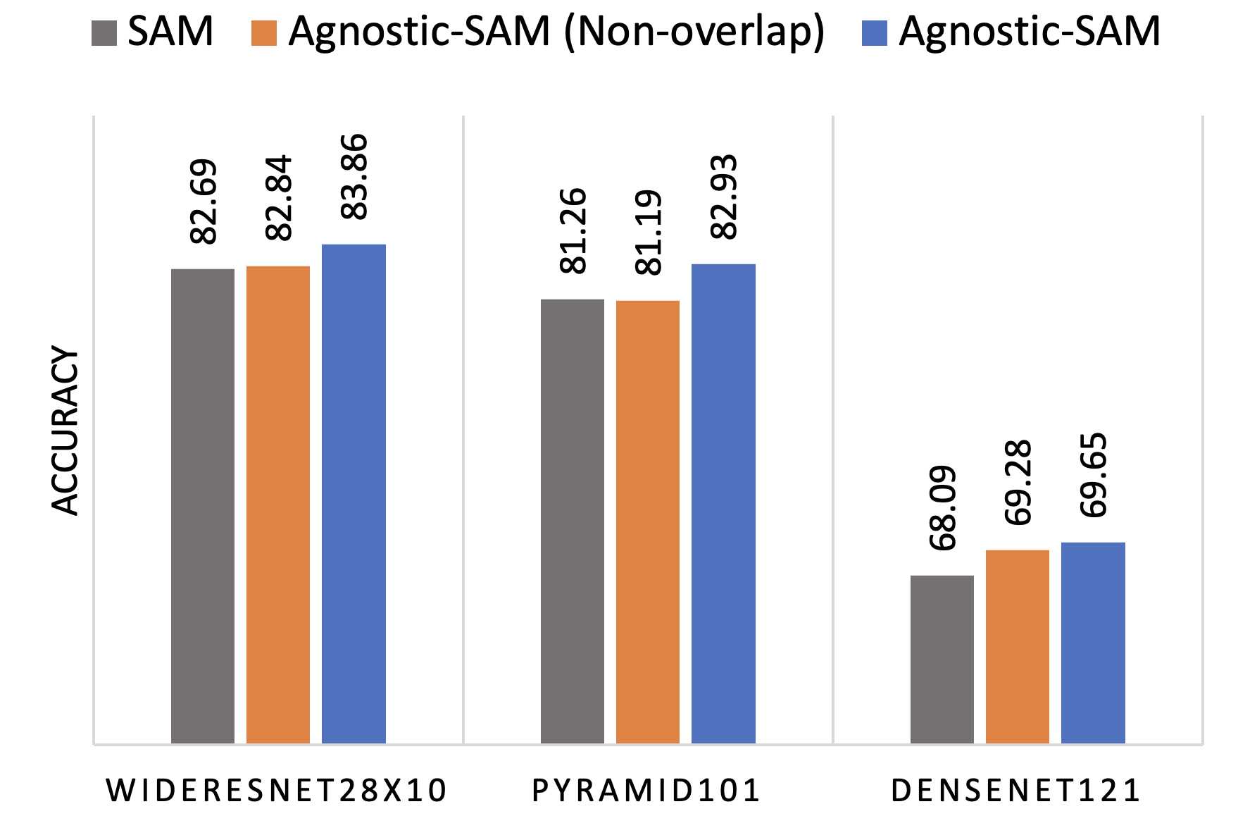
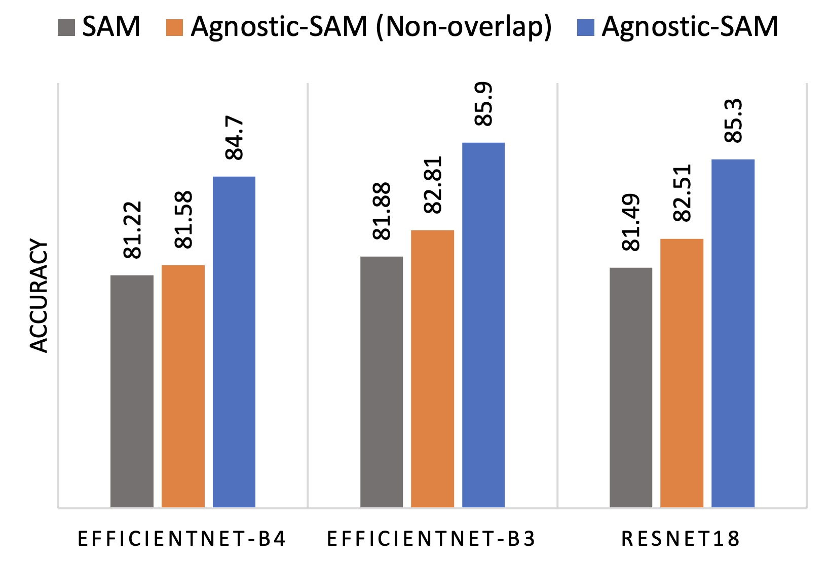
Figure 1: Comparison of setting Agnostic-SAM (Non-overlap), proposed Agnostic-SAM, and the baseline SAM on CIFAR-100 (on the left) and FGVC-Aircraft (on the right)

Table 5: Experiments of AgnosticSAM and its simple version on CIFAR dataset.

Dataset	Method	WideResnet28x10	Pyramid101	Densenet121
CIFAR-10	SAM	96.72 $\pm$ 0.007	96.20 $\pm$ 0.134	91.16 $\pm$ 0.240
	Agnostic-SAM (Simpler)	96.93 $\pm$ 0.021	96.26 $\pm$ 0.101	91.46 $\pm$ 0.154
	Agnostic-SAM	97.17 $\pm$ 0.014	96.30 $\pm$ 0.070	91.17 $\pm$ 0.148
CIFAR-100	SAM	82.69 $\pm$ 0.035	81.26 $\pm$ 0.636	68.09 $\pm$ 0.403
	Agnostic-SAM (Simpler)	83.36 $\pm$ 0.065	82.27 $\pm$ 0.311	68.97 $\pm$ 0.212
	Agnostic-SAM	83.86 $\pm$ 0.077	82.93 $\pm$ 0.247	69.65 $\pm$ 0.226

Effectiveness of sharpness on validation set. As presented in Section 3.3, we first find the perturbed model $\tilde{\theta}_{l}^{v}$ by maximizing the loss on validation samples $B^{v}$, formula (4), then inject the gradient $\nabla_{\theta}\mathcal{L}_{B^{v}}\left(\tilde{\theta}_{l}^{v}\right)$ when find the actual perturbed model $\tilde{\theta}_{l}^{t}$, formula (5). In this way, the actual perturbed model $\tilde{\theta}_{l}^{t}$ maximizes the loss on training samples $B^{t}$ and minimizes the sharpness on $B^{v}$ at the same time. While the proposed method is very effective in enhancing the robustness and generalization error by minimizing sharpness on both training and validation samples, it takes extra training time per epoch.

In this section, we provide a simpler version, in which, the injected gradient when finding the actual perturbed model $\tilde{\theta}_{l}^{t}$ is $\nabla_{\theta}\mathcal{L}_{B^{v}}\left(\theta_{l}\right)$. So that, the simpler version does not require extra steps to perturb the model on validation samples $B^{v}$ and the formula (5) becomes:

$$\tilde{\theta}_{l}^{t}=\theta_{l}+\eta_{1}\nabla_{\theta}\mathcal{L}_{B^{t}}\left(\theta_{l}\right)-\eta_{2}\nabla_{\theta}\mathcal{L}_{B^{v}}\left(\theta_{l}\right)$$

In Table 5, we present experiments with a simpler version of Agnostic-SAM on the CIFAR dataset using various architectures. Impressively, this version consistently outperforms the baseline SAM across all settings by significant margins and achieves results comparable to those of the proposed Agnostic-SAM approach. This demonstrates the effectiveness of our method, which uses the gradient of validation samples as a guide to identify a perturbed model.

5.2 Computation complexity

The training times for SAM and Agnostic-SAM are presented in Table 6. All variations of Agnostic-SAM approach require additional computational steps to calculate the gradients on the validation set in each iteration, compared to SAM. However, in the Non-overlap version, we divide the original training set $S$ into a training set $S^{t}$ and a validation set $S^{v}$ with ratio $|S^{t}|=0.7|S|$ and $|S^{v}|=0.3|S|$, the number of training samples for this version is significantly fewer than the other methods. As a result, the training time per epoch for SAM is slightly longer than for Agnostic-SAM (Non-overlap), but considerably shorter than the other variations of Agnostic-SAM. For different versions of Agnostic-SAM, as the number of gradient steps per epoch increases, both the training time and performance tend to rise accordingly. Considering this is a trade-off for computational complexity and performance in our method.

Table 6: Compare training time (in minutes) per epoch between SAM and Agnostic-SAM on CIFAR-100 and FGVC Aircraft dataset.

Method	WideResnet28x10	Pyramid101	Densenet121
SAM	2.90 $\pm$ 0.01	1.75 $\pm$ 0.00	1.40 $\pm$ 0.04
Agnostic-SAM (Non-overlap)	2.86 $\pm$ 0.00	1.72 $\pm$ 0.01	1.25 $\pm$ 0.02
Agnostic-SAM (Simpler)	3.56 $\pm$ 0.04	2.05 $\pm$ 0.01	1.90 $\pm$ 0.01
Agnostic-SAM	4.78 $\pm$ 0.02	2.86 $\pm$ 0.00	2.25 $\pm$ 0.02
	EfficientNet-B4	EfficientNet-B3	ResNet18
SAM	1.41 $\pm$ 0.02	1.18 $\pm$ 0.01	0.72 $\pm$ 0.03
Agnostic-SAM (Non-overlap)	1.42 $\pm$ 0.03	1.15 $\pm$ 0.00	0.72 $\pm$ 0.01
Agnostic-SAM (Simpler)	1.75 $\pm$ 0.01	1.38 $\pm$ 0.00	0.96 $\pm$ 0.01
Agnostic-SAM	2.36 $\pm$ 0.02	1.71 $\pm$ 0.01	1.13 $\pm$ 0.00

5.3 Analysis of loss landscape

We illustrate the loss landscape of Agnostic-SAM for various architectures on the Flower102 dataset and compare it with the SAM and SGD methods. When training from scratch on EfficientNet-B4, the performance of SAM is unstable across most datasets, often requiring adjustments to several values of $\rho$ to achieve results comparable to those of SGD. This instability is reflected in the loss landscape shown in Figure 2 with high sharpness. In experiments on ResNet18, SAM updates models into wider local minima than SGD (Figure 3). In contrast, Agnostic-SAM consistently leads to a much flatter loss landscape for both the EfficientNet-B4 and ResNet18 models, indicating enhanced stability and potential for better generalization.

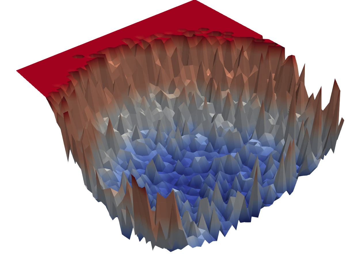
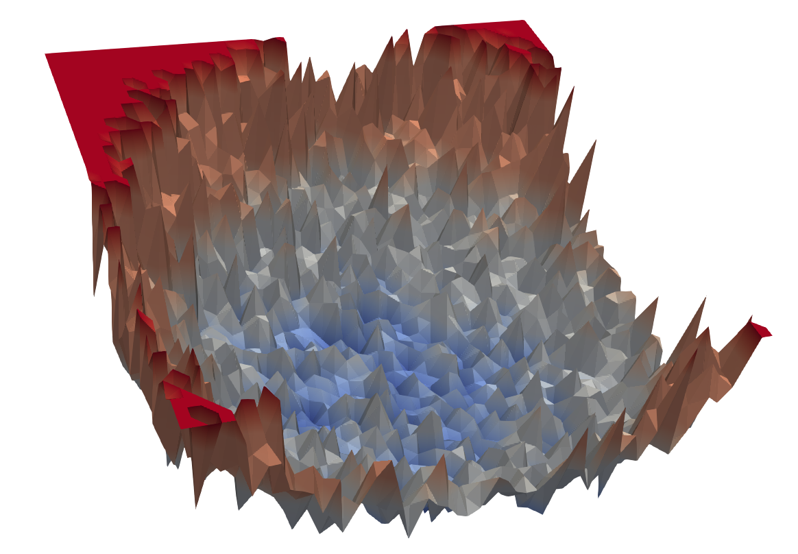
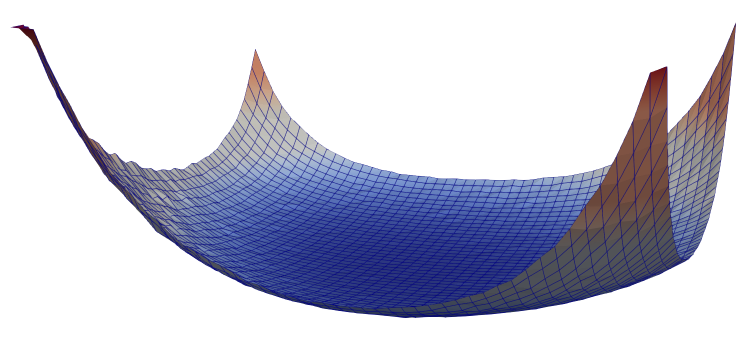
Figure 2: Comparing loss landscape of EffecientNet-B4 trained with (left) SGD, (middle) SAM, and (right) Agnostic-SAM on Flower102 dataset. Evidently, Agnostic-SAM leads the model to a flatter and lower loss area

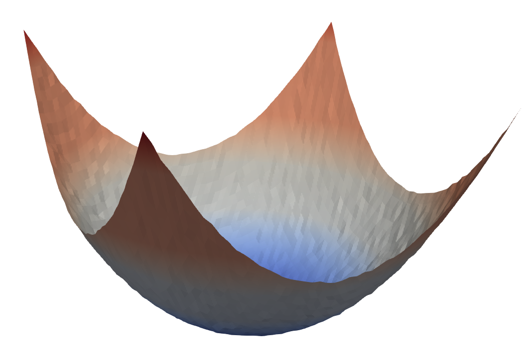
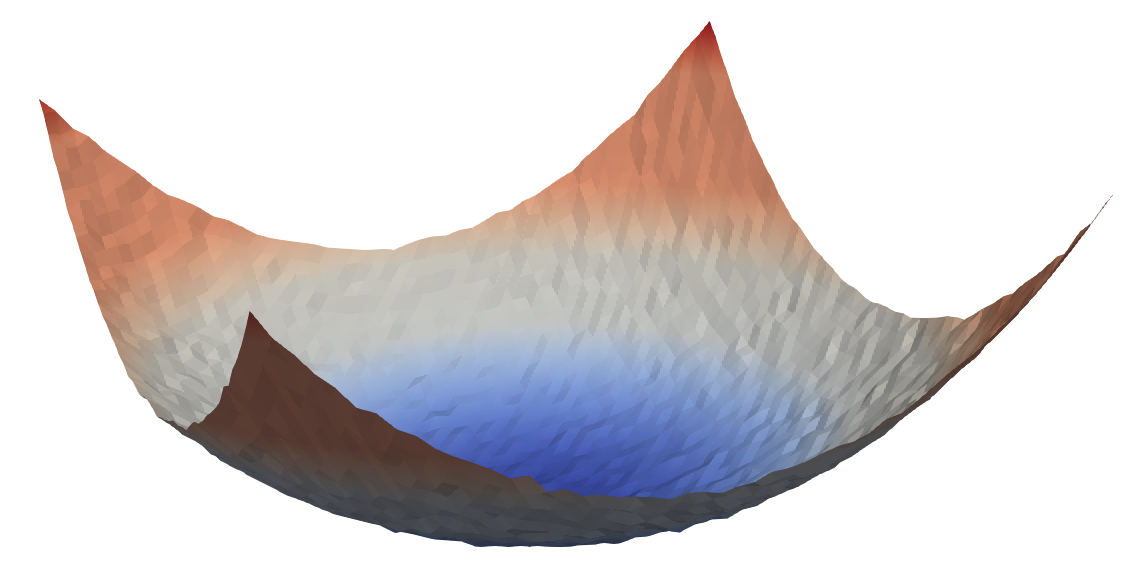
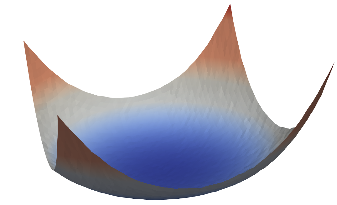
Figure 3: Comparing loss landscape of ResNet18 trained with (left) SGD, (middle) SAM, and (right) Agnostic-SAM on Flower102 dataset. Both SAM and AgnosticSAM update models to flatter regions but AgnosticSAM notably achieves a smoother loss landscape compared to SAM

To further confirm that AgnosticSAM does, in fact, find minima having low curvature, we compute the Hessian for a ResNet18 trained on the Flower102 dataset with loss landscape depicted in Figure 3. The maximum eigenvalue on the log scale is 3.03 with the SGD optimizer, 2.89 with the SAM optimizer, and 2.36 with Agnostic-SAM. This is the same for the experiment with CIFAR-10 on ResNet32. Which, the maximum eigenvalue on the log scale is 4.36 with the SGD optimizer, 4.15 with the SAM optimizer, and notably lower at 3.9 with Agnostic-SAM. This provides additional evidence that Agnostic-SAM consistently leads to the discovery of minima with substantially flatter curvature compared to both SGD and SAM.

6 Conslusion

In this paper, we explore the relationship between SAM and the principles underlying the MAML algorithm in terms of impact on model generalization. Inspired by MAML, we initially approach the problem of learning the best model over a training set from an agnostic viewpoint. From this perspective, we integrate sharpness-aware minimization to construct an agnostic optimization framework and introduce the Agnostic-SAM approach. This novel method optimizes the model towards wider local minima using training data, while concurrently maintaining low loss values on validation data. As a result, Agnostic-SAM is more robust against data shift issues. Through comprehensive experiments, we empirically demonstrate the superiority of Agnostic-SAM over SAM with substantial improvements in model performance across various datasets and under challenging tasks, such as when dealing with noisy labels, or various training settings on small-size datasets.

Appendix A Appendix / supplemental material

In this appendix, we present the proofs in our paper.

A.1 All Proofs

Proof of Theorem 1

Proof.

We use the PAC-Bayes theory in this proof. In PAC-Bayes theory, $\theta$ could follow a distribution, says $P$, thus we define the expected loss over $\theta$ distributed by $P$ as follows:

$$\mathcal{L}_{\mathcal{D}}(\theta,P) =\mathbb{E}_{\theta\sim P}\big{[}\mathcal{L}_{\mathcal{D}}(\theta)\big{]}$$

$$\mathcal{L}_{\mathcal{S}}(\theta,P) =\mathbb{E}_{\theta\sim P}\big{[}\mathcal{L}_{\mathcal{S}}(\theta)\big{]}.$$

For any distribution $P=\mathcal{N}(\mathbf{0},\sigma_{P}^{2}\mathbb{I}_{k})$ and $Q=\mathcal{N}(\theta,\sigma^{2}\mathbb{I}_{k})$ over $\theta\in\mathbb{R}^{k}$, where $P$ is the prior distribution and $Q$ is the posterior distribution, use the PAC-Bayes theorem in [4], for all $\beta>0$, with a probability at least $1-\delta$, we have

$$\mathcal{L}_{\mathcal{D}}(\theta,Q)\leq\mathcal{L}_{\mathcal{S}}(\theta,Q)+\frac{1}{\beta}\Big{[}\mathsf{KL}(Q\|P)+\log\frac{1}{\delta}+\Psi(\beta,N)\Big{]},$$ (9)

where $\Psi$ is defined as

$$\Psi(\beta,N)=\log\mathbb{E}_{P}\mathbb{E}_{\mathcal{D}^{N}}\Big{[}\exp\big{\{}\beta\big{[}\mathcal{L}_{\mathcal{D}}(f_{\theta})-\mathcal{L}_{\mathcal{S}}(f_{\theta})\big{]}\big{\}}\Big{]}.$$

When the loss function is bounded by $L$, then

$$\Psi(\beta,N)\leq\frac{\beta^{2}L^{2}}{8N}.$$

The task is to minimize the second term of RHS of (9), we thus choose $\beta=\sqrt{8N}\frac{\mathsf{KL}(Q\|P)+\log\frac{1}{\delta}}{L}$. Then the second term of RHS of (9) is equal to

$$\sqrt{\frac{\mathsf{KL}(Q\|P)+\log\frac{1}{\delta}}{2N}}\times L.$$

The KL divergence between $Q$ and $P$, when they are Gaussian, is given by formula

$$\mathsf{KL}(Q\|P)=\frac{1}{2}\left[\frac{k\sigma^{2}+\|\theta\|^{2}}{\sigma_{P}^{2}}-k+k\log\frac{\sigma_{P}^{2}}{\sigma^{2}}\right].$$

For given posterior distribution $Q$ with fixed $\sigma^{2}$, to minimize the KL term, the $\sigma_{P}^{2}$ should be equal to $\sigma^{2}+\|\theta\|^{2}/k$. In this case, the KL term is no less than

$$k\log\Big{(}1+\frac{\|\theta_{0}\|^{2}}{k\sigma^{2}}\Big{)}.$$

Thus, the second term of RHS is

$$\sqrt{\frac{\mathsf{KL}(Q\|P)+\log\frac{1}{\delta}}{2N}}\times L\geq\sqrt{\frac{k\log\big{(}1+\frac{\|\theta\|^{2}}{k\sigma^{2}}\big{)}}{4N}}\times L\geq L$$

when $\|\theta\|^{2}>\sigma^{2}\big{\{}\exp(4N/k)-1\big{\}}$. Hence, for any $\|\theta\|_{2}>\sigma^{2}\big{\{}\exp(4N/k)-1\big{\}}$, we have the RHS is greater than the LHS, the inequality is trivial. In this work, we only consider the case:

$$\|\theta\|^{2}<\sigma^{2}\big{(}\exp\{4N/k\}-1\big{)}.$$ (10)

Distribution $P$ is Gaussian centered around $\mathbf{0}$ with variance $\sigma_{P}^{2}=\sigma^{2}+\|\theta\|^{2}/k$, which is unknown at the time we set up the inequality, since $\theta$ is unknown. Meanwhile, we have to specify $P$ in advance, since $P$ is the prior distribution. To deal with this problem, we could choose a family of $P$ such that its means cover the space of $\theta$ satisfying inequality (10). We set

$$c =\sigma^{2}\big{(}1+\exp\{4N/k\}\big{)}$$

$$P_{j} =\mathcal{N}\big{(}0,c\exp\frac{1-j}{k}\mathbb{I}_{k}\big{)}$$

$$\mathfrak{P} :=\big{\{}P_{j}:j=1,2,\ldots\big{\}}$$

Then the following inequality holds for a particular distribution $P_{j}$ with probability $1-\delta_{j}$ with $\delta_{j}=\frac{6\delta}{\pi^{2}j^{2}}$

$$\mathbb{E}_{\theta^{\prime}\sim\mathcal{N}(\theta,\sigma^{2})}\mathcal{L}_{\mathcal{D}}\big{(}f_{\theta^{\prime}}\big{)} \leq\mathbb{E}_{\theta^{\prime}\sim\mathcal{N}(\theta,\sigma^{2})}\mathcal{L}_{\mathcal{S}}\big{(}f_{\theta^{\prime}}\big{)}+\frac{1}{\beta}\left[\mathsf{KL}(Q\|P_{j})+\log\frac{1}{\delta_{j}}+\Psi(\beta,N)\right].$$

Use the well-known equation: $\sum_{j=1}^{\infty}\frac{1}{j^{2}}=\frac{\pi^{2}}{6}$, then with probability $1-\delta$, the above inequality holds with every $j$. We pick

$$j^{*}:=\left\lfloor 1-k\log\frac{\sigma^{2}+\|\theta\|^{2}/k}{c}\right\rfloor=\left\lfloor 1-k\log\frac{\sigma^{2}+\|\theta\|^{2}/k}{\sigma^{2}(1+\exp\{4N/k\})}\right\rfloor.$$

Therefore,

$$1-j^{*}=\left\lceil k\log\frac{\sigma^{2}+\|\theta\|^{2}/k}{c}\right\rceil$$

$$\Rightarrow\quad \log\frac{\sigma^{2}+\|\theta\|^{2}/k}{c}\leq\frac{1-j^{*}}{k}\leq\log\frac{\sigma^{2}+\|\theta_{0}\|^{2}/k}{c}+\frac{1}{k}$$

$$\Rightarrow\quad \sigma^{2}+\|\theta\|^{2}/k\leq c\exp\left\{\frac{1-j^{*}}{k}\right\}\leq\exp(1/k)\big{[}\sigma^{2}+\|\theta\|^{2}/k\big{]}$$

$$\Rightarrow\quad \sigma^{2}+\|\theta\|^{2}/k\leq\sigma_{P_{j^{*}}}^{2}\leq\exp(1/k)\big{[}\sigma^{2}+\|\theta\|^{2}/k\big{]}.$$

Thus the KL term could be bounded as follows

$$\mathsf{KL}(Q\|P_{j^{*}}) =\frac{1}{2}\left[\frac{k\sigma^{2}+\|\theta\|^{2}}{\sigma_{P_{j^{*}}}^{2}}-k+k\log\frac{\sigma_{P_{j^{*}}}^{2}}{\sigma^{2}}\right]$$

$$\leq\frac{1}{2}\left[\frac{k(\sigma^{2}+\|\theta\|^{2}/k)}{\sigma^{2}+\|\theta\|^{2}/k}-k+k\log\frac{\exp(1/k)\big{(}\sigma^{2}+\|\theta\|^{2}/k\big{)}}{\sigma^{2}}\right]$$

$$=\frac{1}{2}\Big{[}k\log\frac{\exp(1/k)\big{(}\sigma^{2}+\|\theta\|^{2}/k\big{)}}{\sigma^{2}}\Big{]}$$

$$=\frac{1}{2}\Big{[}1+k\log\Big{(}1+\frac{\|\theta_{0}\|^{2}}{k\sigma^{2}}\Big{)}\Big{]}$$

For the term $\log\frac{1}{\delta_{j^{*}}}$, with recall that $c=\sigma^{2}\big{(}1+\exp(4N/k)\big{)}$ and

$j^{*}=\left\lfloor 1-k\log\frac{\sigma^{2}+\|\theta\|^{2}/k}{\sigma^{2}(1+\exp\{4N/k\})}\right\rfloor$, we have

$$\log\frac{1}{\delta_{j^{*}}} =\log\frac{(j^{*})^{2}\pi^{2}}{6\delta}=\log\frac{1}{\delta}+\log\Big{(}\frac{\pi^{2}}{6}\Big{)}+2\log(j^{*})$$

$$\leq\log\frac{1}{\delta}+\log\frac{\pi^{2}}{6}+2\log\Big{(}1+k\log\frac{\sigma^{2}\big{(}1+\exp(4N/k)\big{)}}{\sigma^{2}+\|\theta\|^{2}/k}\Big{)}$$

$$\leq\log\frac{1}{\delta}+\log\frac{\pi^{2}}{6}+2\log\Big{(}1+k\log\big{(}1+\exp(4N/k)\big{)}\Big{)}$$

$$\leq\log\frac{1}{\delta}+\log\frac{\pi^{2}}{6}+2\log\Big{(}1+k\big{(}1+\frac{4N}{k}\big{)}\Big{)}$$

$$\leq\log\frac{1}{\delta}+\log\frac{\pi^{2}}{6}+\log(1+k+4N).$$

Hence, the inequality

$$\mathcal{L}_{\mathcal{D}}\Big{(}\theta^{\prime},\mathcal{N}(\theta,\sigma^{2}\mathbb{I}_{k})\Big{)} \leq\mathcal{L}_{\mathcal{S}}\Big{(}\theta^{\prime},\mathcal{N}(\theta,\sigma^{2}\mathbb{I}_{k})\Big{)}+\sqrt{\frac{\mathsf{KL}(Q\|P_{j^{*}})+\log\frac{1}{\delta_{j^{*}}}}{2N}}\times L$$

$$\leq\mathcal{L}_{\mathcal{S}}\Big{(}\theta^{\prime},\mathcal{N}(\theta,\sigma^{2}\mathbb{I}_{k})\Big{)}$$

$$+\frac{L}{2\sqrt{N}}\sqrt{1+k\log\Big{(}1+\frac{\|\theta\|^{2}}{k\sigma^{2}}\Big{)}+2\log\frac{\pi^{2}}{6\delta}+4\log(N+k)}$$

$$\leq\mathcal{L}_{\mathcal{S}}\Big{(}\theta^{\prime},\mathcal{N}(\theta,\sigma^{2}\mathbb{I}_{k})\Big{)}$$

$$+\frac{L}{2\sqrt{N}}\sqrt{k\log\big{(}1+\frac{\|\theta\|^{2}}{k\sigma^{2}}\big{)}+O(1)+2\log\frac{1}{\delta}+4\log(N+k)}.$$

Since $\|\theta^{\prime}-\theta\|^{2}$ is $k$ chi-square distribution, for any positive $t$, we have

$$\mathbb{P}\big{(}\|\theta^{\prime}-\theta\|^{2}-k\sigma^{2}\geq 2\sigma^{2}\sqrt{kt}+2t\sigma^{2}\big{)}\big{)}\leq\exp(-t).$$

By choosing $t=\frac{1}{2}\log(N)$, with probability $1-N^{-1/2}$, we have

$$\|\theta^{\prime}-\theta\|^{2}\leq\sigma^{2}\log(N)+k\sigma^{2}+\sigma^{2}\sqrt{2k\log(N)}\leq k\sigma^{2}\Big{(}1+\sqrt{\frac{\log(N)}{k}}\Big{)}^{2}.$$

By setting $\sigma=\rho\times\big{(}\sqrt{k}+\sqrt{\log(N)}\big{)}^{-1}$, we have $\|\theta^{\prime}-\theta\|^{2}\leq\rho^{2}$. Hence, we get

$$\mathcal{L}_{\mathcal{S}}\Big{(}\theta^{\prime},\mathcal{N}(\theta,\sigma^{2}\mathbb{I}_{k})\Big{)} =\mathbb{E}_{\theta\sim\mathcal{N}(\theta,\sigma^{2}\mathbb{I}_{k})}\mathbb{E}_{\mathcal{S}}\big{[}f_{\theta^{\prime}}\big{]}=\int_{\|\theta^{\prime}-\theta\|\leq\rho}\mathbb{E}_{\mathcal{S}}\big{[}f_{\theta^{\prime}}\big{]}d\mathcal{N}(\theta,\sigma^{2}\mathbb{I})$$

$$+\int_{\|\theta^{\prime}-\theta\|>\rho}\mathbb{E}_{\mathcal{S}}\big{[}f_{\theta^{\prime}}\big{]}d\mathcal{N}(\theta,\sigma^{2}\mathbb{I})$$

$$\leq\Big{(}1-\frac{1}{\sqrt{N}}\Big{)}\max_{\|\theta^{\prime}-\theta\|\leq\rho}\mathcal{L}_{\mathcal{S}}(\theta^{\prime})+\frac{1}{\sqrt{N}}L$$

$$\leq\max_{\|\theta^{\prime}-\theta\|_{2}\leq\rho}\mathcal{L}_{\mathcal{S}}(\theta^{\prime})+\frac{2L}{\sqrt{N}}.$$

It follows that

$$\mathcal{L}_{\mathcal{D}}(\theta)\leq\max_{\|\theta^{\prime}-\theta\|\leq\rho}\mathcal{L}_{\mathcal{S}}(\theta^{\prime}) +\frac{4L}{\sqrt{N}}\Bigg{[}\sqrt{k\log\Big{(}1+\frac{\|\theta\|^{2}}{\rho^{2}}\big{(}1+\sqrt{\log(N)/k}\big{)}^{2}\Big{)}}$$

$$+2\sqrt{\log\big{(}\frac{N+k}{\delta}\big{)}}+O(1)\Bigg{]}$$

$$=\mathcal{L}_{\mathcal{D}}(\theta\mid\mathcal{S})+\frac{4L}{\sqrt{N}}\Bigg{[}\sqrt{k\log\Big{(}1+\frac{\|\theta\|^{2}}{\rho^{2}}\big{(}1+\sqrt{\log(N)/k}\big{)}^{2}\Big{)}}$$

$$+2\sqrt{\log\big{(}\frac{N+k}{\delta}\big{)}}+O(1)\Bigg{]}.$$

By choosing $\theta=\theta^{*}$ and $\mathcal{S}=S^{v}$ hence $N=N^{v}$, we reach the conclusion. ∎

Proof of Theorem 2

Proof.

We have

$$\mathcal{L}_{B^{t}}\left(\tilde{\theta}_{l}^{t}\right)=\mathcal{\mathcal{L}}_{B_{t}}\left(\theta_{l}\right)+\eta_{1}\|\nabla_{\theta}\mathcal{L}_{B^{t}}\left(\theta_{l}\right)\|_{2}^{2}-\eta_{2}\nabla_{\theta}\mathcal{L}_{B^{t}}\left(\theta_{l}\right)\cdot\nabla_{\theta}\mathcal{L}_{B^{v}}\left(\tilde{\theta}_{l}^{v}\right).$$

This follows that

$$\nabla_{\theta}\mathcal{L}_{B^{t}}\left(\tilde{\theta}_{l}^{t}\right) =\nabla_{\theta}\mathcal{\mathcal{L}}_{B_{t}}\left(\theta_{l}\right)+2\eta_{1}H_{B^{t}}\left(\theta_{l}\right)\nabla_{\theta}\mathcal{L}_{B^{t}}\left(\theta_{l}\right)$$

$$-\eta_{2}\left[H_{B^{t}}\left(\theta_{l}\right)\nabla_{\theta}\mathcal{L}_{B^{v}}\left(\tilde{\theta}_{l}^{v}\right)+H_{B^{v}}\left(\tilde{\theta}_{l}^{v}\right)\nabla_{\theta}\mathcal{L}_{B^{t}}\left(\theta_{l}\right)\right],$$

where $H_{B^{t}}\left(\theta_{l}\right)=\nabla_{\theta}^{2}\mathcal{\mathcal{L}}_{B_{t}}\left(\theta_{l}\right)$ and $H_{B^{v}}\left(\tilde{\theta}_{l}^{v}\right)=\nabla_{\theta}^{2}\mathcal{L}_{B^{v}}\left(\tilde{\theta}_{l}^{v}\right)$ are the Hessian matrices.

$$\nabla_{\theta}\mathcal{L}_{B^{v}}\left(\tilde{\theta}_{l}^{v}\right)\cdot\nabla_{\theta}\mathcal{L}_{B^{t}}\left(\tilde{\theta}_{l}^{t}\right) =\nabla_{\theta}\mathcal{\mathcal{L}}_{B_{t}}\left(\theta_{l}\right)\cdot\nabla_{\theta}\mathcal{L}_{B^{v}}\left(\tilde{\theta}_{l}^{v}\right)$$

$$+2\eta_{1}\nabla_{\theta}\mathcal{L}_{B^{v}}\left(\tilde{\theta}_{l}^{v}\right)^{T}H_{B^{t}}\left(\theta_{l}\right)\nabla_{\theta}\mathcal{L}_{B^{t}}\left(\theta_{l}\right)$$

$$-\eta_{2}\nabla_{\theta}\mathcal{L}_{B^{v}}\left(\tilde{\theta}_{l}^{v}\right)^{T}H_{B^{t}}\left(\theta_{l}\right)\nabla_{\theta}\mathcal{L}_{B^{v}}\left(\tilde{\theta}_{l}^{v}\right)$$

$$-\eta_{2}\nabla_{\theta}\mathcal{L}_{B^{v}}\left(\tilde{\theta}_{l}^{v}\right)^{T}H_{B^{v}}\left(\tilde{\theta}_{l}^{v}\right)\nabla_{\theta}\mathcal{L}_{B^{t}}\left(\theta_{l}\right).$$

We now choose $\eta_{1}\leq\frac{\left|\nabla_{\theta}\mathcal{\mathcal{L}}_{B_{t}}\left(\theta_{l}\right)\cdot\nabla_{\theta}\mathcal{L}_{B^{v}}\left(\tilde{\theta}_{l}^{v}\right)\right|}{12\left|\nabla_{\theta}\mathcal{L}_{B^{v}}\left(\tilde{\theta}_{l}^{v}\right)^{T}H_{B^{t}}\left(\theta_{l}\right)\nabla_{\theta}\mathcal{L}_{B^{t}}\left(\theta_{l}\right)\right|}$, we then have

$$\eta_{1}\left|\nabla_{\theta}\mathcal{L}_{B^{v}}\left(\tilde{\theta}_{l}^{v}\right)^{T}H_{B^{t}}\left(\theta_{l}\right)\nabla_{\theta}\mathcal{L}_{B^{t}}\left(\theta_{l}\right)\right|\leq\frac{1}{12}\left|\nabla_{\theta}\mathcal{\mathcal{L}}_{B_{t}}\left(\theta_{l}\right)\cdot\nabla_{\theta}\mathcal{L}_{B^{v}}\left(\tilde{\theta}_{l}^{v}\right)\right|.$$

This further implies

$$\eta_{1}\nabla_{\theta}\mathcal{L}_{B^{v}}\left(\tilde{\theta}_{l}^{v}\right)^{T}H_{B^{t}}\left(\theta_{l}\right)\nabla_{\theta}\mathcal{L}_{B^{t}}\left(\theta_{l}\right)\geq-\frac{1}{12}\left|\nabla_{\theta}\mathcal{\mathcal{L}}_{B_{t}}\left(\theta_{l}\right)\cdot\nabla_{\theta}\mathcal{L}_{B^{v}}\left(\tilde{\theta}_{l}^{v}\right)\right|.$$

Next we choose $\eta_{2}\leq\min\left\{\frac{\left|\nabla_{\theta}\mathcal{\mathcal{L}}_{B_{t}}\left(\theta_{l}\right)\cdot\nabla_{\theta}\mathcal{L}_{B^{v}}\left(\tilde{\theta}_{l}^{v}\right)\right|}{6\left|\nabla_{\theta}\mathcal{L}_{B^{v}}\left(\tilde{\theta}_{l}^{v}\right)^{T}H_{B^{t}}\left(\theta_{l}\right)\nabla_{\theta}\mathcal{L}_{B^{v}}\left(\tilde{\theta}_{l}^{v}\right)\right|},\frac{\left|\nabla_{\theta}\mathcal{\mathcal{L}}_{B_{t}}\left(\theta_{l}\right)\cdot\nabla_{\theta}\mathcal{L}_{B^{v}}\left(\tilde{\theta}_{l}^{v}\right)\right|}{6\left|\nabla_{\theta}\mathcal{L}_{B^{v}}\left(\tilde{\theta}_{l}^{v}\right)^{T}H_{B^{v}}\left(\tilde{\theta}_{l}^{v}\right)\nabla_{\theta}\mathcal{L}_{B^{t}}\left(\theta_{l}\right)\right|}\right\}$, we then have

$$\eta_{2}\left|\nabla_{\theta}\mathcal{L}_{B^{v}}\left(\tilde{\theta}_{l}^{v}\right)^{T}H_{B^{t}}\left(\theta_{l}\right)\nabla_{\theta}\mathcal{L}_{B^{v}}\left(\tilde{\theta}_{l}^{v}\right)\right| \leq\frac{\left|\nabla_{\theta}\mathcal{\mathcal{L}}_{B_{t}}\left(\theta_{l}\right)\cdot\nabla_{\theta}\mathcal{L}_{B^{v}}\left(\tilde{\theta}_{l}^{v}\right)\right|}{6}.$$

$$-\eta_{2}\nabla_{\theta}\mathcal{L}_{B^{v}}\left(\tilde{\theta}_{l}^{v}\right)^{T}H_{B^{t}}\left(\theta_{l}\right)\nabla_{\theta}\mathcal{L}_{B^{v}}\left(\tilde{\theta}_{l}^{v}\right) \geq-\frac{\left|\nabla_{\theta}\mathcal{\mathcal{L}}_{B_{t}}\left(\theta_{l}\right)\cdot\nabla_{\theta}\mathcal{L}_{B^{v}}\left(\tilde{\theta}_{l}^{v}\right)\right|}{6}.$$

$$\eta_{2}\left|\nabla_{\theta}\mathcal{L}_{B^{v}}\left(\tilde{\theta}_{l}^{v}\right)^{T}H_{B^{v}}\left(\tilde{\theta}_{l}^{v}\right)\nabla_{\theta}\mathcal{L}_{B^{t}}\left(\theta_{l}\right)\right| \leq\frac{\left|\nabla_{\theta}\mathcal{\mathcal{L}}_{B_{t}}\left(\theta_{l}\right)\cdot\nabla_{\theta}\mathcal{L}_{B^{v}}\left(\tilde{\theta}_{l}^{v}\right)\right|}{6}.$$

$$-\eta_{2}\nabla_{\theta}\mathcal{L}_{B^{v}}\left(\tilde{\theta}_{l}^{v}\right)^{T}H_{B^{v}}\left(\tilde{\theta}_{l}^{v}\right)\nabla_{\theta}\mathcal{L}_{B^{t}}\left(\theta_{l}\right) \geq-\frac{\left|\nabla_{\theta}\mathcal{\mathcal{L}}_{B_{t}}\left(\theta_{l}\right)\cdot\nabla_{\theta}\mathcal{L}_{B^{v}}\left(\tilde{\theta}_{l}^{v}\right)\right|}{6}.$$

Finally, we yield

$$\nabla_{\theta}\mathcal{L}_{B^{v}}\left(\tilde{\theta}_{l}^{v}\right)\cdot\nabla_{\theta}\mathcal{L}_{B^{t}}\left(\tilde{\theta}_{l}^{t}\right)\geq\nabla_{\theta}\mathcal{\mathcal{L}}_{B_{t}}\left(\theta_{l}\right)\cdot\nabla_{\theta}\mathcal{L}_{B^{v}}\left(\tilde{\theta}_{l}^{v}\right)-\frac{1}{2}\left|\nabla_{\theta}\mathcal{\mathcal{L}}_{B_{t}}\left(\theta_{l}\right)\cdot\nabla_{\theta}\mathcal{L}_{B^{v}}\left(\tilde{\theta}_{l}^{v}\right)\right|.$$

∎

References

- [1] Momin Abbas, Quan Xiao, Lisha Chen, Pin-Yu Chen, and Tianyi Chen. Sharp-maml: Sharpness-aware model-agnostic meta learning. arXiv preprint arXiv:2206.03996, 2022.
- [2] Maruan Al-Shedivat, Trapit Bansal, Yura Burda, Ilya Sutskever, Igor Mordatch, and Pieter Abbeel. Continuous adaptation via meta-learning in nonstationary and competitive environments. In 6th International Conference on Learning Representations, ICLR 2018, Vancouver, BC, Canada, April 30 - May 3, 2018, Conference Track Proceedings. OpenReview.net, 2018.
- [3] Pierre Alquier, James Ridgway, and Nicolas Chopin. On the properties of variational approximations of gibbs posteriors. The Journal of Machine Learning Research, 17(1):8374–8414, 2016.
- [4] Pierre Alquier, James Ridgway, and Nicolas Chopin. On the properties of variational approximations of gibbs posteriors. Journal of Machine Learning Research, 17(236), 2016.
- [5] Maksym Andriushchenko and Nicolas Flammarion. Towards understanding sharpness-aware minimization. In International Conference on Machine Learning, pages 639–668. PMLR, 2022.
- [6] Dara Bahri, Hossein Mobahi, and Yi Tay. Sharpness-aware minimization improves language model generalization. In Proceedings of the 60th Annual Meeting of the Association for Computational Linguistics (Volume 1: Long Papers), pages 7360–7371, Dublin, Ireland, May 2022. Association for Computational Linguistics.
- [7] Peter L. Bartlett and Shahar Mendelson. Rademacher and gaussian complexities: Risk bounds and structural results. J. Mach. Learn. Res., 3(null):463–482, mar 2003.
- [8] Olivier Bousquet and André Elisseeff. Stability and generalization. The Journal of Machine Learning Research, 2:499–526, 2002.
- [9] Junbum Cha, Sanghyuk Chun, Kyungjae Lee, Han-Cheol Cho, Seunghyun Park, Yunsung Lee, and Sungrae Park. Swad: Domain generalization by seeking flat minima. Advances in Neural Information Processing Systems, 34:22405–22418, 2021.
- [10] Jiaxing Chen, Weilin Yuan, Shaofei Chen, Zhenzhen Hu, and Peng Li. Evo-maml: Meta-learning with evolving gradient. Electronics, 12(18), 2023.
- [11] Xiangning Chen, Cho-Jui Hsieh, and Boqing Gong. When vision transformers outperform resnets without pre-training or strong data augmentations. arXiv preprint arXiv:2106.01548, 2021.
- [12] Laurent Dinh, Razvan Pascanu, Samy Bengio, and Yoshua Bengio. Sharp minima can generalize for deep nets. In International Conference on Machine Learning, pages 1019–1028. PMLR, 2017.
- [13] Gintare Karolina Dziugaite and Daniel M. Roy. Computing nonvacuous generalization bounds for deep (stochastic) neural networks with many more parameters than training data. In UAI. AUAI Press, 2017.
- [14] Chelsea Finn, Pieter Abbeel, and Sergey Levine. Model-agnostic meta-learning for fast adaptation of deep networks. In Doina Precup and Yee Whye Teh, editors, Proceedings of the 34th International Conference on Machine Learning, volume 70 of Proceedings of Machine Learning Research, pages 1126–1135. PMLR, 06–11 Aug 2017.
- [15] Chelsea Finn, Kelvin Xu, and Sergey Levine. Probabilistic model-agnostic meta-learning. In Samy Bengio, Hanna M. Wallach, Hugo Larochelle, Kristen Grauman, Nicolò Cesa-Bianchi, and Roman Garnett, editors, Advances in Neural Information Processing Systems 31: Annual Conference on Neural Information Processing Systems 2018, NeurIPS 2018, December 3-8, 2018, Montréal, Canada, pages 9537–9548, 2018.
- [16] Pierre Foret, Ariel Kleiner, Hossein Mobahi, and Behnam Neyshabur. Sharpness-aware minimization for efficiently improving generalization. In International Conference on Learning Representations, 2021.
- [17] Stanislav Fort and Surya Ganguli. Emergent properties of the local geometry of neural loss landscapes. arXiv preprint arXiv:1910.05929, 2019.
- [18] Sepp Hochreiter and Jürgen Schmidhuber. Simplifying neural nets by discovering flat minima. In NIPS, pages 529–536. MIT Press, 1994.
- [19] Stanislaw Jastrzebski, Zachary Kenton, Devansh Arpit, Nicolas Ballas, Asja Fischer, Yoshua Bengio, and Amos J. Storkey. Three factors influencing minima in sgd. ArXiv, abs/1711.04623, 2017.
- [20] Yiding Jiang, Behnam Neyshabur, Hossein Mobahi, Dilip Krishnan, and Samy Bengio. Fantastic generalization measures and where to find them. In ICLR. OpenReview.net, 2020.
- [21] Jean Kaddour, Linqing Liu, Ricardo Silva, and Matt J Kusner. A fair comparison of two popular flat minima optimizers: Stochastic weight averaging vs. sharpness-aware minimization. arXiv preprint arXiv:2202.00661, 1, 2022.
- [22] Nitish Shirish Keskar, Dheevatsa Mudigere, Jorge Nocedal, Mikhail Smelyanskiy, and Ping Tak Peter Tang. On large-batch training for deep learning: Generalization gap and sharp minima. In ICLR. OpenReview.net, 2017.
- [23] Minyoung Kim, Da Li, Shell X Hu, and Timothy Hospedales. Fisher SAM: Information geometry and sharpness aware minimisation. In Kamalika Chaudhuri, Stefanie Jegelka, Le Song, Csaba Szepesvari, Gang Niu, and Sivan Sabato, editors, Proceedings of the 39th International Conference on Machine Learning, volume 162 of Proceedings of Machine Learning Research, pages 11148–11161. PMLR, 17–23 Jul 2022.
- [24] Jungmin Kwon, Jeongseop Kim, Hyunseo Park, and In Kwon Choi. Asam: Adaptive sharpness-aware minimization for scale-invariant learning of deep neural networks. In International Conference on Machine Learning, pages 5905–5914. PMLR, 2021.
- [25] Scott M. Lundberg and Su-In Lee. A unified approach to interpreting model predictions. In Isabelle Guyon, Ulrike von Luxburg, Samy Bengio, Hanna M. Wallach, Rob Fergus, S. V. N. Vishwanathan, and Roman Garnett, editors, Advances in Neural Information Processing Systems 30: Annual Conference on Neural Information Processing Systems 2017, December 4-9, 2017, Long Beach, CA, USA, pages 4765–4774, 2017.
- [26] Thomas Möllenhoff and Mohammad Emtiyaz Khan. Sam as an optimal relaxation of bayes. arXiv preprint arXiv:2210.01620, 2022.
- [27] Sayan Mukherjee, Partha Niyogi, Tomaso A. Poggio, and Ryan M. Rifkin. Statistical learning: Stability is sufficient for generalization and necessary and sufficient for consistency of empirical risk minimization. 2002.
- [28] Behnam Neyshabur, Srinadh Bhojanapalli, David McAllester, and Nati Srebro. Exploring generalization in deep learning. Advances in neural information processing systems, 30, 2017.
- [29] Van-Anh Nguyen, Tung-Long Vuong, Hoang Phan, Thanh-Toan Do, Dinh Phung, and Trung Le. Flat seeking bayesian neural network. In Advances in Neural Information Processing Systems, 2023.
- [30] Henning Petzka, Michael Kamp, Linara Adilova, Cristian Sminchisescu, and Mario Boley. Relative flatness and generalization. In NeurIPS, pages 18420–18432, 2021.
- [31] Hoang Phan, Ngoc Tran, Trung Le, Toan Tran, Nhat Ho, and Dinh Phung. Stochastic multiple target sampling gradient descent. Advances in neural information processing systems, 2022.
- [32] Tomaso Poggio, Ryan Rifkin, Sayan Mukherjee, and Partha Niyogi. General conditions for predictivity in learning theory. Nature, 428(6981):419–422, 2004.
- [33] Zhe Qu, Xingyu Li, Rui Duan, Yao Liu, Bo Tang, and Zhuo Lu. Generalized federated learning via sharpness aware minimization. arXiv preprint arXiv:2206.02618, 2022.
- [34] Aravind Rajeswaran, Chelsea Finn, Sham M. Kakade, and Sergey Levine. Meta-learning with implicit gradients. In Hanna M. Wallach, Hugo Larochelle, Alina Beygelzimer, Florence d’Alché-Buc, Emily B. Fox, and Roman Garnett, editors, Advances in Neural Information Processing Systems 32: Annual Conference on Neural Information Processing Systems 2019, NeurIPS 2019, December 8-14, 2019, Vancouver, BC, Canada, pages 113–124, 2019.
- [35] Marco Túlio Ribeiro, Sameer Singh, and Carlos Guestrin. "why should I trust you?": Explaining the predictions of any classifier. In Balaji Krishnapuram, Mohak Shah, Alexander J. Smola, Charu C. Aggarwal, Dou Shen, and Rajeev Rastogi, editors, Proceedings of the 22nd ACM SIGKDD International Conference on Knowledge Discovery and Data Mining, San Francisco, CA, USA, August 13-17, 2016, pages 1135–1144. ACM, 2016.
- [36] Tuan Truong, Hoang-Phi Nguyen, Tung Pham, Minh-Tuan Tran, Mehrtash Harandi, Dinh Phung, and Trung Le. Rsam: Learning on manifolds with riemannian sharpness-aware minimization, 2023.
- [37] Vladimir Naumovich Vapnik. Statistical learning theory. In Adaptive and Learning Systems for Signal Processing, Communications, and Control. Wiley, 1998.
- [38] Bokun Wang, Zhuoning Yuan, Yiming Ying, and Tianbao Yang. Memory-based optimization methods for model-agnostic meta-learning and personalized federated learning. Journal of Machine Learning Research, 24(145):1–46, 2023.
- [39] Colin Wei, Sham Kakade, and Tengyu Ma. The implicit and explicit regularization effects of dropout. In International conference on machine learning, pages 10181–10192. PMLR, 2020.