D-Gril: End-to-End Topological Learning with $2$-parameter Persistence

Abstract

End-to-end topological learning using $1$-parameter persistence is well known. We show that the framework can be enhanced using $2$-parameter persistence by adopting a recently introduced $2$-parameter persistence based vectorization technique called Gril. We establish a theoretical foundation of differentiating Gril producing D-Gril. We show that D-Gril can be used to learn a bifiltration function on standard benchmark graph datasets. Further, we exhibit that this framework can be applied in the context of bio-activity prediction in drug discovery.

1 Introduction

In recent years, persistent homology, one of the flagship concepts of Topological Data Analysis (TDA), has found its use in many fields such as neuroscience, material science, sensor networks, shape recognition, gene expression data analysis and many more Giunti et al. (2022). The performance of machine learning models such as Graph Neural Networks (GNNs) can be enhanced by augmenting topological information captured by persistent homology (Hofer et al., 2017; Dehmamy et al., 2019; Carrière et al., 2020; Horn et al., 2022). Classical persistent homology, also known as $1$-parameter persistence, captures the evolution of topological structures in a simplicial complex $K$ following a filter function $f\colon K\to\mathbb{R}$. The evolution of topological structures, in this case, can be completely characterized and compactly represented as persistence diagrams or equivalently barcodes Zomorodian & Carlsson (2004); Edelsbrunner et al. (2002). These persistence diagrams or barcodes can be vectorized Bubenik (2015); Reininghaus et al. (2015); Adams et al. (2017); Hofer et al. (2019); Carrière et al. (2020); Kim et al. (2020) and used in machine learning pipelines. In most applications, the simplicial complex $K$ is given and the choice of the filter function $f$ depends on the application. Choosing an appropriate filter function can be challenging. To avoid this, in Hofer et al. (2020), the authors proposed an end-to-end learning framework to learn the filter function rather than relying on making the right choice. They showed that learning the filter function performs better than the standard choices of filter functions on many graph datasets.

To obtain richer topological information, we can consider an $\mathbb{R}^{n}$-valued filter function instead of a scalar filter function. This leads to the structure of a multiparameter persistence module instead of $1$-parameter persistence module. Multiparameter persistence modules, unlike their $1$-parameter counterparts, can not be classified completely using a discrete invariant Carlsson et al. (2009). Consequently, vectorizing multiparameter persistence modules while retaining as much topological information as possible has become a challenging problem. There are many recent works in this direction which use incomplete invariants such as rank invariant Carlsson et al. (2009) or equivalently fibered barcodes Lesnick & Wright (2015), multiparameter persistence images Carrière & Blumberg (2020), multiparameter persistence landscapes Vipond (2020), multiparameter persistence kernel Corbet et al. (2019), vectorization of signed barcodes Loiseaux et al. (2023), topological fingerprinting for virtual screening using multidimensional persistence Demir et al. (2022), effective multidimensional persistence Chen et al. (2023) or generalized rank invariant Xin et al. (2023). The authors, in all these works, show that $2$-parameter persistence methods perform better than $1$-parameter persistence methods on many graph and time-series datasets, suggesting that an $\mathbb{R}^{2}$-valued filter function, indeed, captures richer topological information than a scalar filter function. However, in all these works, one needs to make a suitable choice for an $\mathbb{R}^{2}$-valued filter function. Akin to the $1$-parameter setup, learning the filter function rather than choosing a filter function can prove to be more informative and beneficial for the task at hand.

In this paper, we propose an end-to-end learning framework using $2$-parameter persistent homology based on the vectorization Gril introduced by Xin et al. (2023). We show that Gril is piecewise affine and give an explicit formula for the differential of Gril. The results discussed in Davis et al. (2020); Carrière et al. (2021) help us to show the convergence of stochastic sub-gradient descent on Gril. We use these results to build a differentiable topological layer D-Gril, consequently an end-to-end learning pipeline. We use D-Gril for bio-activity prediction and provide experimental results. One of the key advantages of using TDA in the context of bio-activity prediction is its ability to capture and analyze the shape and structural characteristics of molecules in a manner that traditional methods might overlook. Molecules possess intricate shapes and topological features that directly influence their interactions with biological targets. TDA can uncover these subtleties, allowing for a deeper understanding of structure-activity relationships. We also show that D-Gril can be used, more generally, for bifiltration learning on graphs and provide experimental results where we compare with existing multiparameter persistent homology methods on benchmark graph datasets.

To the best of our knowledge, end-to-end topological learning with multiparameter persistence has not been investigated in the literature. In concurrent work, Scoccola et al. (2024) address this question by developing a general framework suitable for a class of invariants of multiparameter persistence. Our approach is specific to GRIL but is more direct and yields a simpler line of argument.

2 Overview

Our main construct is Gril, introduced in Xin et al. (2023) for vectorizing a $2$-parameter persistence module. Gril is defined in the same spirit as persistence landscapes Bubenik (2015), introduced for $1$-parameter persistence. The landscape uses the rank function over the interval decomposition known for $1$-parameter persistence modules. To extend the concept to $2$-parameter persistence modules, one faces two main challenges: (i) in general, persistence modules beyond $1$-parameter may not decompose into intervals, (ii) the usual rank function cannot be defined for intervals that are not rectangular. Gril solves (i) by defining the landscape function over a fixed set of two-dimensional intervals called $\ell$-worms instead of the support of the indecomposables of the modules, and solves (ii) by considering a generalized version of the rank function termed as generalized rank (Definition 3.3). An $\ell$-worm is an interval in $\mathbb{R}^{2}$ parameterized by a center point $\mathbf{p}$, a length $\ell$, and a width $d$. In practice, a discrete version of the $\ell$-worms is used (Definition 4.1 and Figure 1), which allows for the efficient computation of the generalized rank over them using zigzag persistence Dey et al. (2024).

An interesting property of the generalized rank over intervals is that it monotonically decreases as the intervals get larger. Thus, given fixed parameters $k>0$ and $\ell>0$, the width $d$ of an $\ell$-worm can be increased until the generalized rank over the worm drops below $k$. The maximum value of the width thus obtained, $d_{\mathbf{p}}$, is the value of Gril at the worm center point $\mathbf{p}$ for $k$ and $\ell$. In practice, $s$ center points $\mathbf{p}_{1},\cdots,\mathbf{p}_{s}$ are sampled from the plane, and each center point $\mathbf{p}_{i}$ contributes an entry $d_{\mathbf{p}_{i}}$ in the final Gril vector. We refer the reader to Xin et al. (2023) for a detailed description and an algorithm to compute Gril.

Gril yields a vector representation of the 2-parameter persistence module formed from a given simplicial complex and a bifiltration function (formally defined in section 3). However, there is no provision to learn this bifiltration function. Often, it is difficult to choose the right filtration function that elicits the relevant information present in the data. For $1$-parameter persistence, learnt filter functions have been shown to perform better than the filter functions popularly chosen in TDA. To learn a suitable bifiltration function, we build a differentiable layer called D-Gril. We show in section 5 that the learnt bifiltration function performs better than some of the popular bifiltration functions known in TDA supporting the need for end-to-end learning.

Towards this goal, we study the differentiability of Gril, seeking a closed form equation for its differential wherever defined. This, in turn, enables us to differentiate through the Gril computation, which is necessary for the topological layer in our end-to-end learning framework. In this regard, we draw upon the results discussed in Carrière et al. (2021); Davis et al. (2020) for the conditions required for convergence of stochastic sub-gradient descent. We show that our framework satisfies these conditions and, consequently, that stochastic sub-gradient descent converges almost surely.

3 Background

We review and recall some definitions and results in this section. Section 3.1 primarily consists of concepts in multiparameter persistent homology. Section 3.2 consists of concepts and results that establish the conditions required for the convergence of stochastic sub-gradient descent. Section 3.3 contains some background which is required to prove that Gril satisfies these conditions.

3.1 Multiparameter persistent homology

In this subsection, we briefly review the concepts in multiparameter persistent homology. We focus, primarily, on 2-parameter persistent homology. For detailed definitions, refer Edelsbrunner & Harer (2010); Dey & Wang (2022). We begin by recalling the definition of a simplicial complex. Given a finite vertex set $V$, a simplicial complex $K=K(V)$ defined on this vertex set is a collection of subsets of $V$ such that if a subset $\sigma\subseteq V$ is in $K$, then all proper subsets $\tau\subset\sigma$ are also in $K$. Each element in $K$ with cardinality $k+1$ is called a $k$-simplex or simply a simplex. A graph is a simplicial complex where $V$ is the vertex set of the graph and $K$ consists of edges and vertices of the graph. A filtration is a collection of simplicial complexes $\{K_{\mathbf{x}}\}_{\mathbf{x}\in\mathbb{R}}$ indexed by the reals, with the property that $K_{\mathbf{x}}\subseteq K_{\mathbf{y}}$ for each $\mathbf{x}\leq\mathbf{y}$. Extending this definition to collections of complexes indexed by $\mathbb{R}^{2}$ with the product partial order ($\mathbf{x}\leq\mathbf{y}\in\mathbb{R}^{2}$ if $x_{1}\leq y_{1}$ and $x_{2}\leq y_{2}$), we get a bifiltration.

Definition 3.1 (Bifiltration).

A bifiltration is a collection of simplicial complexes $\{K_{\mathbf{x}}\}_{\mathbf{x}\in\mathbb{R}^{2}}$ where $K_{\mathbf{x}}\subseteq K_{\mathbf{y}}$ for all comparable $\mathbf{x}\leq\mathbf{y}\in\mathbb{R}^{2}$.

Let $K$ be a simplicial complex and $f\colon K\to\mathbb{R}^{2}$ be a map with the property that $f(\sigma)\leq f(\tau)\in\mathbb{R}^{2}$ for all $\sigma\subseteq\tau$. For each $\mathbf{x}\in\mathbb{R}^{2}$, let $K_{\mathbf{x}}\coloneqq\{\sigma\in K\colon f(\sigma)\leq\mathbf{x}\}$. Clearly, $K_{\mathbf{x}}\subseteq K_{\mathbf{y}}$ for all comparable $\mathbf{x}\leq\mathbf{y}\in\mathbb{R}^{2}$. The resulting bifiltration, denoted $\{K^{f}_{\mathbf{x}}\}_{\mathbf{x}\in\mathbb{R}^{2}}$, is called the sub-level set bifiltration of the bifiltration function $f$.

A filtration in the $1$-parameter case induces a persistence module, obtained by considering the inclusion-induced linear maps between the vector spaces given by the homology groups of the simplicial complexes comprising the filtration. Similarly, we obtain a $2$-parameter persistence module from a bifiltration.

Definition 3.2 (2-parameter persistence module).

A 2-parameter persistence module is an assignment of finite-dimensional vector spaces $M_{\mathbf{x}}$ for each $\mathbf{x}\in\mathbb{R}^{2}$, and of linear maps $M_{\mathbf{x}\leq\mathbf{y}}\colon M_{\mathbf{x}}\to M_{\mathbf{y}}$ for all comparable $\mathbf{x}\leq\mathbf{y}\in\mathbb{R}^{2}$, with the properties that $M_{\mathbf{x}\leq\mathbf{x}}=\text{id}$ and $M_{\mathbf{y}\leq\mathbf{z}}\circ M_{\mathbf{x}\leq\mathbf{y}}=M_{\mathbf{x}\leq\mathbf{z}}$ for all $\mathbf{\mathbf{x}\leq\mathbf{y}}\leq\mathbf{z}\in\mathbb{R}^{2}$.

Readers familiar with category theory can recognize that a 2-parameter persistence module is a functor $M\colon\mathbb{R}^{2}\to\textbf{vec}_{\mathbb{F}}$ where the poset $\mathbb{R}^{2}$ is regarded as a category and $\textbf{vec}_{\mathbb{F}}$ denotes the category of finite-dimensional vector spaces over a field $\mathbb{F}$.

Given a bifiltration $\{K_{\mathbf{x}}\}_{\mathbf{x}\in\mathbb{R}^{2}}$, we consider $H_{i}(K_{\mathbf{x}})$, the $i$th homology group of the simplicial complex $K_{\mathbf{x}}$ over a field $F$, say $\mathbb{Z}_{2}$. Then, for each inclusion $K_{\mathbf{x}}\subseteq K_{\mathbf{y}}$, we get an induced linear map $H_{i}(K_{\mathbf{x}})\to H_{i}(K_{\mathbf{y}})$. By this assignment, we get a 2-parameter persistence module.

Let $\{K^{f}_{\mathbf{x}}\}_{\mathbf{x}\in\mathbb{R}^{2}}$ be a sub-level set bifiltration. Then the 2-parameter persistence module $M$ obtained by the homology assignment is called the 2-parameter persistence module induced by $f$, and we denote it as $M_{f}$.

As mentioned in Section 2, Gril vectorization uses the concept of generalized rank introduced by Kim & Mémoli (2021), which we define below formally.

Definition 3.3 (Generalized Rank).

Let $M$ be a 2-parameter persistence module. The restriction of $M$ to an interval $I$ of $\mathbb{R}^{2}$ (see Appendix A), denoted by $M|_{I}$, is the diagram formed by the collection of vector spaces $M_{\mathbf{x}}$ for $\mathbf{x}\in I$ and linear maps $M_{\mathbf{x}\leq\mathbf{y}}$ for all comparable $\mathbf{x}\leq\mathbf{y}\in I$. Then, the generalized rank of $M$ over $I$ is defined as the rank of the canonical linear map from the limit $\varprojlim M|_{I}$ to colimit $\varinjlim M|_{I}$:

$$\mathsf{rk}^{M}(I)\coloneqq\text{rank}\left(\varprojlim M|_{I}\rightarrow\varinjlim M|_{I}\right).$$

We refer the reader to MacLane (1971) for the definitions of limit, colimit, and the construction of the canonical limit-to-colimit map. Intuitively, generalized rank captures the number of independent topological features supported over the interval $I$. It can be computed efficiently for $2$-parameter persistence modules using an algorithm in Dey et al. (2024).

Remark 3.4.

In the special case where $I$ is a rectangle, $\mathsf{rk}^{M}(I)$ is the rank of the linear map $M_{\mathbf{u}\leq\mathbf{v}}$ from the lower left corner $\mathbf{u}$ of the rectangle to the upper right corner $\mathbf{v}$.

3.2 Stochastic sub-gradient descent

In this subsection, we briefly review the result and the conditions under which stochastic sub-gradient descent converges as shown in Davis et al. (2020). In  Carrière et al. (2021), authors use this result in the setting of $1$-parameter persistent homology and show that stochastic sub-gradient descent converges in that case.

Given a loss function $\mathcal{L}$ with the objective of minimizing it, consider the differential inclusion

$$\dot{\mathbf{z}}(t)\in-\partial\mathcal{L}(\mathbf{z}(t))\hskip 8.5359pt\text{ for almost every }t.$$

The solutions $\mathbf{z}(t)$ are the trajectories of the sub-gradient of $\mathcal{L}$ which can be approximated by the standard stochastic sub-gradient descent method given by:

$$\mathbf{x}_{k+1}=\mathbf{x}_{k}-\alpha_{k}(\mathbf{y}_{k}+\mathbf{\zeta}_{k}),\hskip 8.5359pt\mathbf{y}_{k}\in\partial\mathcal{L}(\mathbf{x}_{k}),$$ (1)

where the sequence $(\alpha_{k})_{k}$ is the learning rate and $(\zeta_{k})_{k}$ is a sequence of random variables or “noise”. Davis et al. (2020) establish that under mild technical assumptions (Assumption C in Davis et al. (2020)) on these two sequences, the stochastic sub-gradient method converges almost surely to critical points of $\mathcal{L}$ if $\mathcal{L}$ is locally Lipschitz and Whitney stratifiable.

Proposition 3.5 (Corollary 5.9 Davis et al. (2020)).

Let $f\colon\mathbb{R}^{d}\to\mathbb{R}$ be a locally Lipschitz function that is $C^{d}$-stratifiable. Consider the iterates $\{\mathbf{x}_{k}\}_{k\geq 1}$ produced by the stochastic sub-gradient method (Eq (1)) and suppose Assumption C of Davis et al. (2020) holds. Then, almost surely, every limit point of the iterates $\{\mathbf{x}_{k}\}_{k\geq 1}$ is critical for $f$ and the function values $\{f(\mathbf{x}_{k})\}_{k\geq 1}$ converge.

3.3 o-minimal geometry

It is known that any definable function in an o-minimal structure admits a Whitney $C^{p}$ stratification for all $p\geq 1$ Van den Dries & Miller (1996). We recall the definitions of o-minimal structure and definable function here.

Definition 3.6 (o-minimal structure).

An o-minimal structure on $\mathbb{R}$ is a collection $\{S_{n}\}_{n\in\mathbb{N}}$ where each $S_{n}$ is a set of subsets of $\mathbb{R}^{n}$ such that:

1. $S_{1}$ is exactly the collection of finite union of points and intervals.

2. $S_{n}$ contains all the sets of the form $\{\mathbf{x}\in\mathbb{R}^{n}\colon p(\mathbf{x})=0\}$ where $p$ is a polynomial on $\mathbb{R}^{n}$.

3. $S_{n}$ is a Boolean sub-algebra of $\mathbb{R}^{n}$ for all $n$.

4. If $A\in S_{n}$ and $B\in S_{m}$, then $A\times B\in S_{n+m}$.

5. If $\pi\colon\mathbb{R}^{n+1}\to\mathbb{R}^{n}$ is the canonical projection onto the first $n$-coordinates, then for $A\in S_{n+1}$, $\pi(A)\in S_{n}$.

A subset $A\in S_{n}$ for some $n\in\mathbb{N}$ is known as a definable set in the o-minimal structure. Let $A\in S_{n}$ be given. A function $f\colon A\to\mathbb{R}^{m}$ is said to be definable if the graph of the function in $\mathbb{R}^{n+m}$ is a definable set.

We note that all semi-algebraic functions are definable. In fact, the author in, Wilkie (1996), shows that there exists an o-minimal structure that simultaneously contains all semi-algebraic sets and the graph of the exponential function. The authors in Davis et al. (2020) use this result to show that a neural network, being a composition of definable functions, is definable (Corollary 5.11 Davis et al. (2020)). For readers not familiar with the notion of definable functions, it is sufficient to know that a piecewise affine map is definable as it is semi-algebraic.

4 Differentiability of Gril

We begin this section by proving that Gril is a piecewise affine map in section 4.1. Gril being piecewise affine leads us to the fact that stochastic sub-gradient converges almost surely on Gril, which is discussed in section 4.2. In section 4.3, we give an explicit formula for the differential of Gril. We conclude this section by pointing out some practical issues that arise while implementing this differentiable pipeline and discussing the solutions in section 4.4.

4.1 Gril as a piecewise affine map

We begin by recalling the definitions of $\ell$-worm and Gril.

Definition 4.1 (discrete $\ell$-worm, Xin et al. (2023)).

Let $\boxed{\mathbf{p}}_{d}\coloneqq\{\mathbf{w}:\|\mathbf{p}-\mathbf{w}\|_{\infty}\leq d\}$ be the $d$-square centered at $\mathbf{p}\in\mathbb{R}^{2}$ with side $2d$. Given $\ell\geq 1\text{ and }d>0$, the $\ell$-worm, $\boxed{\mathbf{p}}_{d}^{\ell}$, is defined as the union of all $d$-squares $\boxed{\mathbf{q}}_{d}$ centered at some point $\mathbf{q}$ on the off-diagonal line segment $\mathbf{p}\pm\alpha\cdot(1,-1)$ with $\alpha=j\cdot d$ where $j\in\{1,\ldots,\ell-1\}$.

Refer to Figure 1 for a $2$-worm.

Definition 4.2 (Gril, Xin et al. (2023)).

For a 2-parameter persistence module $M$, the Generalized Rank Invariant Landscape (Gril) is a function $\lambda^{M}:\mathbb{R}^{2}\times\mathbb{N}_{+}\times\mathbb{N}_{+}\rightarrow\mathbb{R}$ defined as

$$\lambda^{M}(\mathbf{p},k,\ell)\coloneqq\sup\left\{d\geq 0\colon\mathsf{rk}^{M}\left(\boxed{\mathbf{p}}^{\ell}_{d}\right)\geq k\right\}.$$

Fixing the bifiltration function $f$ and $k,\ell$, the landscape $\lambda^{M}$ provides a function $\lambda^{M_{f}}_{k,\ell}:\mathbb{R}^{2}\rightarrow\mathbb{R}$, $\mathbf{\mathbf{\mathbf{p}}}\mapsto\lambda^{M_{f}}(\mathbf{\mathbf{\mathbf{p}}},k,\ell)$. The Gril vector is the vector of values of $\lambda^{M_{f}}_{k,\ell}$ evaluated at a set of chosen sample points $\{\mathbf{p}_{1},\ldots,\mathbf{p}_{s}\}\subset\mathbb{R}^{2}$.

Let $K$ be a simplicial complex with $n$ simplices, labelled $\sigma_{1},\sigma_{2},\ldots,\sigma_{n}$. A bifiltration function $f\colon K\to\mathbb{R}^{2}$ can be viewed as a vector $\mathbf{v}_{f}\in\mathbb{R}^{2n}$ where, for $k=1,\ldots,n$, $\mathbf{v}_{f}[2k-1]=f_{x}(\sigma_{k})$ and $\mathbf{v}_{f}[2k]=f_{y}(\sigma_{k})$. Here, $f_{x}(\sigma)$ and $f_{y}(\sigma)$ denote the $x$- and $y$-coordinates of the vector $f(\sigma)$ respectively. Notice that the vectors in $\mathbb{R}^{2n}$ that correspond to a valid bifiltration function form a convex cone. We work with this set of vectors in $\mathbb{R}^{2n}$. In this setting, the authors in Xin et al. (2023) show that Gril is Lipschitz continuous in the following sense.

Proposition 4.3.

Let $X$ be a discrete space with $|X|=n$. For fixed $k,\ell,\mathbf{p}$, let $\Lambda_{k,\ell}^{\mathbf{p}}\colon\mathbb{R}^{2n}\to\mathbb{R}$ be the map $\mathbf{v}_{f}\mapsto\lambda^{M_{f}}_{k,\ell}(\mathbf{p})$. Then, $\Lambda^{\mathbf{p}}_{k,\ell}$ is Lipschitz continuous.

By Rademacher’s theorem Federer (2014), the above proposition also says that $\Lambda^{\mathbf{p}}_{k,\ell}$ is differentiable almost everywhere.

Let $\mathcal{G}_{k,\ell}\colon\mathbb{R}^{2n}\to\mathbb{R}^{s}$ be the map defined as:

$$\mathcal{G}_{k,\ell}(v_{f})=\left[\Lambda_{k,\ell}^{\mathbf{p}_{1}}(\mathbf{v}_{f}),\Lambda_{k,\ell}^{\mathbf{p}_{2}}(\mathbf{v}_{f}),\ldots,\Lambda_{k,\ell}^{\mathbf{p}_{s}}(\mathbf{v}_{f})\right]^{T}$$ (2)

where $\{\mathbf{p}_{j}\}_{j=1}^{s}$ are the $s$ sampled center points. We drop the $k,\ell$ and refer to $\mathcal{G}_{k,\ell}$ as $\mathcal{G}$ whenever $k,\ell$ are well understood. We note that $\mathcal{G}$ is also a function of the center points $\mathbf{p}_{j}$ for all $j$. We show that $\mathcal{G}$ is piecewise affine.

For notational convenience, in what follows we denote $f_{x}(\sigma)$ as $\sigma^{x}$ and $f_{y}(\sigma)$ as $\sigma^{y}$, and we call them the simplex coordinates of $\sigma$. Similarly, we denote the $x$-coordinate and $y$-coordinate of $\mathbf{p}$ as $\mathbf{p}^{x}$ and $\mathbf{p}^{y}$ respectively.

We observe that, if there are two simplices $\sigma_{i},\sigma_{j}$ such that for some $\rho\in\mathbb{Z}\text{ and }0\leq\rho\leq\ell$ and $a,b\in\{x,y\}$, one has $|\sigma_{i}^{a}-\mathbf{p}_{t}^{a}|=\rho\cdot|\sigma_{j}^{b}-\mathbf{p}_{t}^{b}|$ then, say for $a=x$ and $b=y$, the point representing the vector $\mathbf{v}_{f}$ lies on a hyperplane in $\mathbb{R}^{2n}$:

$$\left\{\mathbf{v}\in\mathbb{R}^{2n}\colon\left|\mathbf{v}[2i-1]-\mathbf{p}_{t}^{x}\right|=\rho\cdot\left|\mathbf{v}[2j]-\mathbf{p}_{t}^{y}\right|\right\}.$$

Corresponding to each such pair of simplex coordinates, we get one hyperplane. Here, in the example, we chose one simplex coordinate to be $x$-coordinate and the other to be $y$-coordinate. This, however, need not always be the case: we can have all four possible combinations of $x$- and $y$-coordinates, corresponding to each of which we get a hyperplane. The exact formula of all such hyperplanes is given in Appendix A. Combining all these hyperplanes, we get an arrangement $\mathcal{H}$ of hyperplanes in $\mathbb{R}^{2n}$ Goodman & O’Rourke (2004). The arrangement $\mathcal{H}$ partitions $\mathbb{R}^{2n}$ into relatively open $r$-cells, $r\in\{0,\ldots,2n\}$. We observe that this arrangement induces an affine stratification $\mathcal{S}_{\mathcal{H}}$ (refer Leygonie et al. (2021) for the formal definition) of $\mathbb{R}^{2n}$ where the $r$-dimensional strata are precisely the $r$-cells.

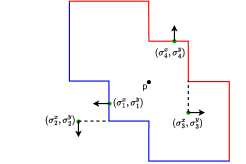
Figure 1: A 2-worm with lower boundary colored in blue and upper boundary colored in red. The figure also shows the possible cases of constraining simplex coordinates; $\sigma_{1}$ is a case of lower $x$-constraining simplex coordinate because the $x$-coordinate $\sigma_{1}^{x}$ constrains the lower boundary of the worm and prevents the worm from expanding further to the left; $\sigma_{2}$ is an example of lower $y$-constraining simplex coordinate because $\sigma_{2}^{y}$ also constrains the lower boundary of the worm and prevents the worm from expanding downwards. Similarly, $\sigma_{3}$ and $\sigma_{4}$ are upper $x$-constraining and upper $y$-constraining respectively. The arrows depict the gradient directions as described in Theorem 4.7.

In the following we prove that $\mathcal{G}$ is a piecewise affine map relative to this arrangement, meaning that it is affine on each stratum of $\mathcal{S}_{\mathcal{H}}$. To this end, we introduce the notions of upper boundary, lower boundary, and constraining simplex coordinate for an $\ell$-worm. These notions will allow us to characterize the strata of $\mathcal{S}_{\mathcal{H}}$ in terms of conditions on the bifiltration function. We give an intuitive explanation of these concepts below using Figure 1. Formal definitions are given in Appendix A.

In Figure 1, a $2$-worm is shown with its lower boundary colored in blue and its upper boundary in red. As depicted, the lower boundary consists of the part of the boundary that is in the lower half of the worm, while the upper boundary consists of the rest of the boundary. More precisely, a point belongs to the lower boundary (resp. upper boundary) if the open lower-set (resp. upper-set) of the point does not intersect the worm.

For an intuitive understanding of constraining simplex coordinate, consider the Gril value $d$ of an $\ell$-worm centered at $\mathbf{p}$ for a given rank $k$. It follows from Definition 4.2 that there exists at least one simplex $\sigma$ such that $\sigma^{x}$ or $\sigma^{y}$ prevents the worm from expanding any further to have a Gril value more than $d$ at $\mathbf{p}$. The coordinate in question (either $\sigma^{x}$ or $\sigma^{y}$) is called a constraining simplex coordinate for the $\ell$-worm centered at $\mathbf{p}$. Here, by preventing the worm from expanding, we mean that if the worm were to expand then the value of the generalized rank over the worm would drop below the given value of rank $k$. Note that an $\ell$-worm can have multiple constraining simplex coordinates, including some coming from the same simplex $\sigma$.

We can characterize the top-dimensional ($2n$-dimensional) strata of $\mathcal{S}_{\mathcal{H}}$ in terms of conditions on constraining simplex coordinates for $\ell$-worms, and consequently, in terms of conditions on the bifiltration functions.

Proposition 4.4.

The top-dimensional strata of $\mathcal{S}_{\mathcal{H}}$ consist precisely of those bifiltration functions that have a unique constraining simplex coordinate for each $\ell$-worm.

We state the main theorem of this subsection.

Theorem 4.5.

Let $K$ be a simplicial complex with $n$ simplices. Let $k,\ell\in\mathbb{N}$, and let $\{\mathbf{p}_{j}\}_{j=1}^{s}$ be the $s$ sampled center points for the $\ell$-worms. Then, $\mathcal{G}$, as defined in Eq.(2), is a piecewise affine map relative to the arrangement $\mathcal{H}$.

Overview of the proof: $\mathcal{G}$ depends affinely on the simplex coordinates in each top-dimensional stratum, because there is a unique constraining simplex coordinate for each $\ell$-worm. By continuity of $\mathcal{G}$ (Proposition 4.3), the restriction of $\mathcal{G}$ to each (affine) lower dimensional stratum is affine.

4.2 Stochastic sub-gradient descent

In our machine learning pipeline, the Gril map $\mathcal{G}$ is post-composed with a loss function $N\colon\mathbb{R}^{s}\to\mathbb{R}$, derived e.g. from some neural network. In the corollary below, we give sufficient conditions on $N$ that ensure the convergence of stochastic sub-gradient descent on $N\circ\mathcal{G}$.

Corollary 4.6.

If $N\colon\mathbb{R}^{s}\to\mathbb{R}$ is definable and locally Lipschitz continuous, then, under the assumptions of Proposition 3.5 and Theorem 4.5, stochastic sub-gradient descent on $N\circ\mathcal{G}$ converges almost surely to critical points of $N\circ\mathcal{G}$.

Overview of the proof: In the discussion towards the end of section 3.2, we saw that any piecewise affine map is definable. Since $\mathcal{G}$ is piecewise affine, it is locally Lipschitz and definable. We know that the composition of two definable functions is definable, and that the composition of two locally Lipschitz functions is locally Lipschitz. These facts, put together with Proposition 3.5, immediately lead to the fact that stochastic sub-gradient descent converges almost surely to critical points of $N\circ\mathcal{G}$.

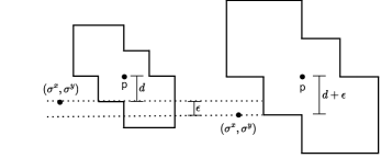
Figure 2: An intuitive understanding of the gradient assignment described in Theorem 4.7. The $y$-coordinate $\sigma^{y}$ is at a distance of $d$ from the $y$-coordinate of $\mathbf{p}$ in the left figure; $\sigma$ is the only constraining simplex for the $2$-worm. In the figure on the right, $\sigma^{y}$ has reduced by $\epsilon$ and is now at a distance $d+\epsilon$ from $\mathbf{p}^{y}$. As a consequence, the value of Gril increases from $d$ to $d+\epsilon$. Thus, $\frac{\partial\Lambda^{\mathbf{p}}_{k,\ell}(\mathbf{v}_{f})}{\partial\sigma^{y}}=-1$ as described in Theorem 4.7.

4.3 Differential of Gril

In order to back-propagate gradients through the Gril computation, we need an explicit formula for the differential of $\mathcal{G}$. Such a formula is needed only in the top-dimensional strata, where $\mathcal{G}$ is actually smooth. In lower-dimensional strata, sub-gradients can be approximated using, e.g., gradient sampling Burke et al. (2020).

In section 4.1, we saw that $\mathcal{G}$ is piecewise affine, which implies that its differential is constant in each top-dimensional stratum. In order to compute it, we need to determine the sign of the gradient at different simplex coordinates. To do so, given a worm, we distinguish between simplex coordinates that constrain the lower boundary of the worm and those that constrain its upper boundary. Since each simplex has two coordinates, $x$ and $y$, and these can be constraining either the upper boundary or the lower boundary, we get four different cases: lower $x$-constraining, lower $y$-constraining, upper $x$-constraining and upper $y$-constraining. All these cases are shown in Figure 1.

We deduce an explicit formula for the differential of $\mathcal{G}$ in the top-dimensional strata.

Theorem 4.7.

Let $K$ be a simplicial complex with $n$ simplices. Let $k,\ell\in\mathbb{N}$ and $\{\mathbf{p}_{j}\}_{j=1}^{s}$ be the $s$ sampled center points for the $\ell$-worms. Then, the differential of $\mathcal{G}$ at any $\mathbf{v}_{f}$ in a top-dimensional stratum is given by:

$$\begin{pmatrix}\frac{\partial\Lambda^{\mathbf{p}_{1}}_{k,\ell}(\mathbf{v}_{f})}{\partial\sigma_{1}^{x}}&\frac{\partial\Lambda^{\mathbf{p}_{1}}_{k,\ell}(\mathbf{v}_{f})}{\partial\sigma_{1}^{y}}&\frac{\partial\Lambda^{\mathbf{p}_{1}}_{k,\ell}(\mathbf{v}_{f})}{\partial\sigma_{2}^{x}}&\ldots&\frac{\partial\Lambda^{\mathbf{p}_{1}}_{k,\ell}(\mathbf{v}_{f})}{\partial\sigma_{n}^{y}}\\ \vdots&&&&\vdots\\ \frac{\partial\Lambda^{\mathbf{p}_{s}}_{k,\ell}(\mathbf{v}_{f})}{\partial\sigma_{1}^{x}}&\ldots&\ldots&&\frac{\partial\Lambda^{\mathbf{p}_{s}}_{k,\ell}(\mathbf{v}_{f})}{\partial\sigma_{n}^{y}}\end{pmatrix}_{s\times 2n}$$

where,

$$\frac{\partial\Lambda^{\mathbf{p}_{j}}_{k,\ell}(\mathbf{v}_{f})}{\partial\sigma_{i}^{x}}=\begin{cases}-1,&\text{if }\sigma_{i}\text{ is lower x-constraining for }\boxed{\mathbf{p}_{j}}^{\ell}_{d_{j}},\\ +1,&\text{if }\sigma_{i}\text{ is upper x-constraining for }\boxed{\mathbf{p}_{j}}^{\ell}_{d_{j}},\\ 0,&\text{otherwise},\end{cases}$$

$$\frac{\partial\Lambda^{\mathbf{p}_{j}}_{k,\ell}(\mathbf{v}_{f})}{\partial\sigma_{i}^{y}}=\begin{cases}-1,&\text{if }\sigma_{i}\text{ is lower y-constraining for }\boxed{\mathbf{p}_{j}}^{\ell}_{d_{j}}\\ +1,&\text{if }\sigma_{i}\text{ is upper y-constraining for }\boxed{\mathbf{p}_{j}}^{\ell}_{d_{j}}\\ 0,&\text{otherwise},\end{cases}$$

and $d_{j}$ is the Gril value at $\mathbf{p}_{j}$.

Recall that each $\mathbf{v}_{f}$ in a top-dimensional stratum of $\mathcal{S}_{\mathcal{H}}$ corresponds to a bifiltration function $f$ with a unique constraining simplex. Refer to Figure 2 for an intuitive explanation about the sign of the gradient and the different cases in Theorem 4.7, as shown by the arrows in Figure 1.

Corollary 4.8.

Given the conditions of Theorem 4.7, partial derivatives of $\mathcal{G}$ with respect to $\mathbf{p}_{j}^{x}$ and $\mathbf{p}_{j}^{y}$ also exist and are given by:

$$\frac{\partial\Lambda^{\mathbf{p}_{j}}_{k,\ell}(\mathbf{v}_{f})}{\partial\mathbf{p}_{j}^{x}}=\begin{cases}+1,&\text{if there exists a lower x-constraining simplex for }\boxed{\mathbf{p}_{j}}^{\ell}_{d_{j}},\\ -1,&\text{if there exists an upper x-constraining simplex for }\boxed{\mathbf{p}_{j}}^{\ell}_{d_{j}},\\ 0,&\text{otherwise,}\end{cases}$$

$$\frac{\partial\Lambda^{\mathbf{p}_{j}}_{k,\ell}(\mathbf{v}_{f})}{\partial\mathbf{p}_{j}^{y}}=\begin{cases}+1,&\text{if there exists a lower y-constraining simplex for }\boxed{\mathbf{p}_{j}}^{\ell}_{d_{j}},\\ -1,&\text{if there exists an upper y-constraining simplex for }\boxed{\mathbf{p}_{j}}^{\ell}_{d_{j}},\\ 0,&\text{otherwise}.\end{cases}$$

4.4 Practical Considerations

In section 4.1 we saw that $\mathcal{G}$ is piecewise affine and in section 4.2 we deduced that stochastic sub-gradient descent converges almost surely to critical points of $N\circ\mathcal{G}$ for any definable and locally Lipschitz loss function $N$. We gave an explicit formula for the differential of Gril in the top-dimensional strata in section 4.3, and at the beginning of that section we argued that gradient sampling can be used to approximate sub-gradients in lower-dimensional strata. In practice, for the sake of computational efficiency, we use a simple variant of gradient sampling, which consists of sampling a single nearby point and taking its gradient.

So far, we considered a bifiltration function on the entire simplicial complex $K$. However, in practice, we may need to extend the filtration function to the entire simplicial complex based on filtration function values on certain simplices. For example, in a lower-star filtration, the filtration function values on the higher dimensional simplices are dictated by the filtration function values on the vertices of the simplicial complex. In a Rips filtration, the filtration function values on the vertices are 0, while the filtration function values on higher dimensional simplices are dictated by the filtration function values on the edges.

In such scenarios, the bifiltration function $f$ is given on a subcomplex $L$ of the simplicial complex $K$. This is extended to a bifiltration function $\bar{f}$ on the entire simplicial complex in a piecewise constant manner. We use the example of lower-star bifiltration to show how our framework fits to this type of scenario. Let $f\colon K^{0}\to\mathbb{R}^{2}$ be a function on the vertices of the simplicial complex $K$ with $m$ vertices and $n$ simplices. The map $f$ is extended to a piecewise constant map $\bar{f}\colon K\to\mathbb{R}^{2}$ as follows: for an edge $e=(u,v)$, we let $\bar{f}_{x}(e)=\max\{f_{x}(u),f_{x}(v)\}$ and $\bar{f}_{y}(e)=\max\{f_{y}(u),f_{y}(v)\}$; the values on higher dimensional simplices are defined inductively. Notice that for each simplex $\sigma\in K$, there is a maximal $x$-vertex and a maximal $y$-vertex, the vertices that give the $x$ and $y$-values to the simplex respectively. We know that $f$ can be represented as a vector $\mathbf{v}_{f}\in\mathbb{R}^{2m}$ and $\bar{f}$ as a vector $\mathbf{v}_{\bar{f}}\in\mathbb{R}^{2n}$ after ordering the simplices of $K$. Consider the map $q\colon\mathbb{R}^{2m}\to\mathbb{R}^{2n}$ given by $q(\mathbf{v}_{f})=\mathbf{v}_{\bar{f}}$. The map $q$ is piecewise affine and thus, $\mathcal{G}\circ q$ is piecewise affine as well. Therefore, we can apply stochastic sub-gradient descent on $N\circ\mathcal{G}\circ q$ with analogous convergence guarantees.

Observe that we get an arrangement of hyperplanes on $\mathbb{R}^{2m}$, $\mathcal{H}_{q}$, analogous to $\mathcal{H}$ on $\mathbb{R}^{2n}$ that we saw in the previous subsections. On the top-dimensional cells of $\mathcal{H}_{q}$, the differential of $q$ is well-defined and constant and expressions analogous to the ones in Theorem 4.7 can be derived, and the chain rule can be used for back-propagating gradients. As mentioned previously, we use a simple form of gradient sampling to approximate sub-gradients when the gradient is not well-defined. For the experimental section that follows, $N$ is a neural network with one of the standard choices for loss functions, which is definable as discussed towards the end of section 3.3.

5 Experiments

In this section, we present the experimental results on various bio-activity prediction datasets and benchmark graph datasets. We begin the section by describing our experimental setup and then move on to a brief description of bio-activity prediction datasets followed by experimental results on those datasets. Towards the end of the section, we show that D-Gril can be, more generally, applied in the context of bifiltration learning on standard benchmark graph datasets. We compare with existing multiparameter persistent homology methods on these datasets. All the reported accuracy/ROC-AUC scores, in this section, are $5$-fold cross-validated scores.

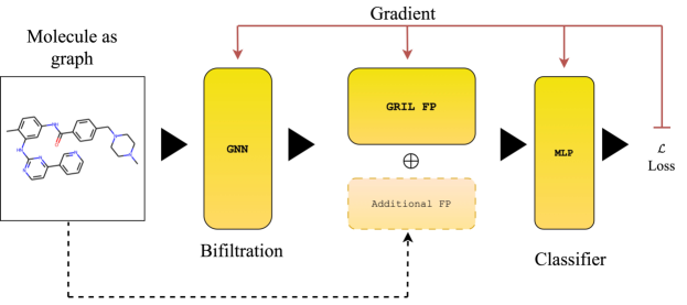
Figure 3: Architecture choice for bio-activity prediction; the bifiltration fuction $f$ is learnt compared to the standard multiparameter pipeline; $\oplus$ denotes concatenation of vectors.

5.1 Experimental Setup

Every instance in each dataset is an attributed graph with a label associated with it. We use a Graph Isomorphism Network (GIN) Xu et al. (2019) to obtain a bifiltration function over the vertices. We consider the lower-star bifiltration of this function. This gives us a bifiltration function on the entire graph, which we denote as $f$. Let $\mathbf{v}_{f}$ denote the vector representation of $f$ which we get after ordering the simplices of the graph. We divide the range of $f$ into a grid of size $100\times 100$. We randomly initialize the $s$ center points from this grid and compute the vector $\mathcal{G}_{k,\ell}(\mathbf{v}_{f})$ (Eq. (2)) for $k=1,2,3$ and $\ell=2$ at these center points. For computational efficiency, we restrict the center points and the boundaries of the worms to the grid. Note that the bifiltration function values are not restricted to the grid. This ensures that the differential of Gril is computed in $\mathbb{R}^{2n}$ and the steps of stochastic sub-gradient descent are updated in $\mathbb{R}^{2n}$. This vector $\mathcal{G}_{k,\ell}(\mathbf{v}_{f})$ is fed to a $3$-layer Multilayer Perceptron (MLP) classifier and the loss is back-propagated through the Gril computation according to the gradient described in Section 4. Note that the positions of the $s$ center points are also optimized as the gradient can be backpropagated to the coordinates the center points as well. Additional details and hyperparameter choices are given in Appendix B.

5.2 Bio-activity Prediction Datasets

The data is extracted from the ChEMBL database Gaulton et al. (2012); Davies et al. (2015). Each dataset contains the SMILES Weininger (1988) encoding of a novel drug (compound), and activity pairs for a target of interest. For example, the EGFR dataset contains all the molecules that have been tested against epidermal growth factor receptor (EGFR) kinase, and their measured bio-activity. The SMILES encodings of the molecules are then converted to graphs with Molfeat Noutahi et al. (2023). Bio-activity is measured in half maximal inhibitory concentration $(IC_{50})$, which qualitatively indicates how much a drug is needed, in vitro, to inhibit a particular process by $50\%$. To facilitate the comparison of $IC_{50}$ values, it is common practice to convert $IC_{50}$ to $pIC_{50}=-\log_{10}(IC_{50})$, expressed in molar units. Threshold for activity cutoff $pIC_{50}=6.3$ is used throughout the paper. More details about the datasets are given in Appendix B.

Dataset	GIN	GIN-Gril	D-Gril
EGFR	$55.60\pm 8.61$	$58.39\pm 2.51$	$\mathbf{65.38\pm 5.34}$
ERRB2	$57.06\pm 8.58$	$61.28\pm 3.66$	$\mathbf{69.24\pm 5.06}$
CHEMBL1163125	$58.48\pm 4.37$	$54.13\pm 1.09$	$\mathbf{65.69\pm 1.57}$
CHEMBL2148	$52.88\pm 0.91$	$50.24\pm 0.18$	$\mathbf{53.13\pm 3.70}$
CHEMBL4005	$55.90\pm 4.63$	$51.85\pm 3.55$	$\mathbf{59.34\pm 5.70}$

Table 1: Test ROC-AUC on ChEMBL datasets. D-Gril performs better than GIN with sum pooling and Gril with bifiltration obtained from pre-trained GIN.

In the first set of experiments, we compare D-Gril with (i) a standard GNN model–GIN with sum-pooling, (ii) with GIN and Gril as a readout layer. Note that for the results on GIN-Gril, Gril is used as a passive readout layer, i.e., we obtain a bifiltration function from a pre-trained GIN (pre-trained for graph classification on the same dataset) and compute Gril on it. We use the exact same pipeline as GIN-Gril and train it end-to-end using D-Gril and report the results in the last column. The classifier, $3$-layer MLP, is the same for all the experiments. Refer to Figure 3 for the pipeline. From Table 1, we can see that adding topological information after GIN has been trained can improve the performance in some cases and need not be beneficial in others. However, it is clear from the table that adding topological information in an end-to-end framework appears to be beneficial for bio-activity prediction.

Further, we perform a series of experiments where we augment other popular molecular fingerprints such as ECFP and Morgan3 (Rogers & Hahn, 2010; Morgan, 1965) with the D-Gril framework. In these experiments, we compare the performance of the model with and without D-Gril augmentation. We report the results in Table 2. We can see from the table that augmenting with D-Gril seems to, generally, increase the performance of the model. Indeed, fingerprints such as ECFP and Morgan3 can essentially represent an infinite number of different molecular features, including stereochemical information (Rogers & Hahn, 2010) but they are not effective in capturing global features of molecules such as size and shape (Capecchi et al., 2020). Combining D-Gril with these fingerprints augments the model with topological information, leading to an improved performance.

Dataset	ECFP	ECFP+D-Gril	Morgan3	Morgan3+D-Gril
EGFR	$83.27\pm 1.10$	$\mathbf{84.37\pm 1.22}$	$82.39\pm 1.35$	$\mathbf{83.57\pm 1.40}$
ERRB2	$83.53\pm 1.31$	$\mathbf{86.24\pm 2.27}$	$83.19\pm 1.26$	$\mathbf{85.51\pm 1.47}$
CHEMBL1163125	$83.94\pm 1.23$	$\mathbf{86.33\pm 0.67}$	$83.55\pm 1.20$	$\mathbf{84.85\pm 0.82}$
CHEMBL203	$81.74\pm 0.90$	$\mathbf{81.86\pm 0.90}$	$80.85\pm 1.32$	$\mathbf{81.64\pm 0.45}$
CHEMBL2148	$73.96\pm 2.59$	$\mathbf{74.13\pm 2.33}$	$72.79\pm 1.97$	$\mathbf{74.50\pm 2.61}$
CHEMBL279	$76.72\pm 1.34$	$\mathbf{78.75\pm 0.77}$	$76.76\pm 0.50$	$\mathbf{78.05\pm 1.18}$
CHEMBL2815	$73.69\pm 1.53$	$\mathbf{76.51\pm 1.48}$	$73.42\pm 0.56$	$\mathbf{75.22\pm 2.85}$
CHEMBL4005	$\mathbf{80.45\pm 1.30}$	$80.41\pm 0.97$	$79.95\pm 1.30$	$\mathbf{80.55\pm 0.82}$
CHEMBL4722	$78.05\pm 1.64$	$\mathbf{78.51\pm 1.83}$	$78.76\pm 1.37$	$\mathbf{79.17\pm 1.30}$

Table 2: Test ROC-AUC scores on ChEMBL datasets; augmenting ECFP and Morgan3 fingerprints with D-Gril increases the classification performance for most of the datasets.

Dataset	D-Gril	Gril	MP-I	MP-L	MP-K	P
MUTAG	$\mathbf{85.09\pm 5.99}$	$83.49\pm 3.64$	$74.99\pm 2.79$	$82.42\pm 3.72$	$79.27\pm 2.45$	$66.50\pm 0.87$
PROTEINS	$69.45\pm 4.11$	$66.31\pm 2.34$	$70.80\pm 3.09$	$\mathbf{70.80\pm 1.31}$	$61.70\pm 2.98$	$59.57\pm 0.08$
DHFR	$61.24\pm 4.37$	$\mathbf{61.64\pm 1.66}$	$60.98\pm 0.10$	$61.11\pm 0.25$	$60.98\pm 0.10$	$60.98\pm 0.10$
COX2	$78.16\pm 0.41$	$78.16\pm 0.41$	$78.16\pm 0.41$	$78.16\pm 0.41$	$78.16\pm 0.41$	$78.16\pm 0.41$
IMDB-BINARY	$\mathbf{58.90\pm 1.90}$	$50.00\pm 0.00$	$56.60\pm 2.94$	$50.00\pm 0.00$	$50.30\pm 1.12$	$50.00\pm 0.00$

Table 3: Test accuracies of D-Gril on benchmark graph datasets.

5.3 Benchmark Graph Datasets

D-Gril can be used more generally for filtration learning on graph datasets. We perform a series of experiments with benchmark graph datasets such as Mutag, Proteins, Dhfr, Cox2 Morris et al. (2020) and compare with existing multiparameter persistence methods. Details about the datasets are given in Appendix B. We report the results in Table 3. For a valid comparison, we use a $3$-layer MLP as the classifier for all the multiparameter signatures. Hence, the numbers reported look different from the ones in Xin et al. (2023), Carrière & Blumberg (2020) where the authors consider XGBoost (Chen & Guestrin, 2016). In fact, in Xin et al. (2023), the authors show that XGBoost performs much better than a $3$-layer MLP classifier for Gril vectors on these datasets. We can see from the table that learning the bifiltration function seems to perform better than multiparameter persistence methods on popular choices of bifiltration functions on most datasets. We can also see that D-Gril performs better than Gril, supporting our argument for an end-to-end learning framework. We report the training times in Table 4. We can see from the table that the approach is feasible and can be used in practice.

Dataset	Time(hh:mm:ss)
MUTAG	00:05:08
COX2	00:11:34
DHFR	00:16:48
PROTEINS	00:30:03

Table 4: Reported times are training times per fold averaged over 5 folds that we used for training. All the experiments have been performed on a machine with AMD EPYC 7313 16-Core Processor and NVIDIA A10 GPU.

In order to visualize the learnt bifiltration function, we plot it and the D-Gril vectors for $H_{0}$ and $H_{1}$ and compare it with the plots of Heat-Kernel Signature-Ricci Curvature (HKS-RC) bifiltration function and corresponding Gril vectors on two randomly selected graph instances from the Proteins dataset. The figures are shown in Appendix B.

6 Conclusion

In this paper, we propose a differentiable framework using Gril, a $2$-parameter persistent homology based vectorization. We show that stochastic sub-gradient descent converges almost surely on Gril, and we compute an explicit formula for the differential of Gril. We use this formula to back-propagate gradients through the Gril computation, yielding the differentiable framework D-Gril. We use D-Gril to show that adding topological information in an end-to-end manner is beneficial for bio-activity prediction. Further, we show that D-Gril can be used in a more general setting, for filtration learning on graphs. Our results indicate that learnt bifiltration functions on graphs, generally, give a better performance than the standard choices for bifiltration functions. This indicates, and we believe, that learning filtration functions can prove to be more informative for topological methods in machine learning. We hope that this work sparks interest and motivates research in this direction.

7 Acknowledgement

This work is supported partially by NSF grants CCF 2049010 and DMS 2301360.

Appendix A Formal Definitions and Proofs

Definition A.1 (Interval in $\mathbb{R}^{2}$).

An interval in ${\mathbb{R}^{2}}$ is a subset $\emptyset\neq I\subseteq{\mathbb{R}^{2}}$ that satisfies the following:

1. If $\mathbf{u},\mathbf{v}\in I$ and $\mathbf{u}\leq\mathbf{w}\leq\mathbf{v}$, then $\mathbf{w}\in I$;

2. If $\mathbf{u},\mathbf{v}\in I$, then there exists a finite sequence ($\mathbf{u}=\mathbf{u}_{0},\mathbf{u}_{1},,...,\mathbf{u}_{m}=\mathbf{v})\in I$ so that every consecutive points $\mathbf{u}_{i},\mathbf{u}_{i+1}$ are comparable in the partial order for $i\in\{0,\ldots,m-1\}$.

Definition A.2 (Upper-set and lower-set).

Given a poset $(P,\leq)$, the upper-set of $x\in P$ is defined as

$$x^{\uparrow P}\coloneqq\{y\in P\colon x\leq y\}.$$

Similarly, the lower-set of $x\in P$ is defined as

$$x^{\downarrow P}\coloneqq\{y\in P\colon y\leq x\}.$$

Definition A.3 (Upper and lower boundary of $\ell$-worm).

Let an $\ell$-worm centered at $\mathbf{p}$ with width $d$, denoted as $\boxed{\mathbf{p}}_{d}^{\ell}$, be given. A point $\mathbf{t}$ is said to be on the upper boundary of the worm if $\mathring{\mathbf{t}}^{(\uparrow\mathbb{R}^{2})}\cap\boxed{\mathbf{p}}_{d}^{\ell}=\emptyset$ where $\mathring{\mathbf{t}}^{(\uparrow\mathbb{R}^{2})}$ denotes the open upper-set of $\mathbf{t}$ in $\mathbb{R}^{2}$. The collection of all such points constitutes the upper boundary of the worm. Similarly, a point $t$ is on the lower boundary if $\mathring{\mathbf{t}}^{(\downarrow\mathbb{R}^{2})}\cap\boxed{\mathbf{p}}_{d}^{\ell}=\emptyset$ and the collection of all such points constitutes the lower boundary of the worm.

Definition A.4 (Constraining Simplex Coordinate).

Given a bifiltration function $f$, $k\in\mathbb{N}$, $\ell\in\mathbb{N},\mathbf{p}\in\mathbb{R}^{2}$ let $\lambda^{M_{f}}(\mathbf{p},k,\ell)=d$. Let $\sigma$ be a simplex with $\boxed{\mathbf{p}}^{\ell}_{d}\cap f(\sigma)^{\uparrow\mathbb{R}^{2}}\neq\emptyset$ such that one of the following two conditions holds:

1. $f_{x}(\sigma)=\mathbf{p}_{x}\pm j\cdot d$

2. $f_{y}(\sigma)=\mathbf{p}_{y}\pm j\cdot d$

for some $j\in\{1,\ldots,\ell-1\}$. Then $\sigma$ is called a constraining simplex for $\boxed{\mathbf{p}}^{\ell}_{d}$. If $\sigma$ satisfies (1), $\sigma^{x}(=f_{x}(\sigma))$ is the constraining simplex coordinate or equivalently, $\sigma$ is called x-constraining and if it satisfies (2), $\sigma^{y}(=f_{y}(\sigma))$ is the constraining simplex coordinate or equivalently $\sigma$ is called y-constraining.

Definition A.5.

Let $f$ be a bifiltration function. Let $\sigma$ be a constraining simplex for $\boxed{\mathbf{p}}^{\ell}_{d}$. $\sigma$ is said to be an upper constraining simplex if $f(\sigma)^{\uparrow\mathbb{R}^{2}}$ intersects only the upper boundary of $\boxed{\mathbf{p}}^{\ell}_{d}$. $\sigma$ is called a lower constraining simplex if $f(\sigma)^{\uparrow\mathbb{R}^{2}}$ intersects both lower and upper boundary of $\boxed{\mathbf{p}}^{\ell}_{d}$. $\sigma$ is said to be lower $x$-constraining if $\sigma$ is lower constraining and $\sigma^{x}$ is the constraining simplex coordinate. The notions of upper $x$-constraining, lower $y$-constraining and upper $y$-constraining are similarly defined.

Formulae for the arrangement of hyperplanes. Here, we provide the formulae for the different hyperplanes that form the arrangement of hyperplanes described in section 4. Recall that we have $s$ sampled center points and a bifiltration function on $n$ simplices, $\sigma_{1},\ldots,\sigma_{n}$.

1. $$\left\{\mathbf{v}\in\mathbb{R}^{2n}\colon|\mathbf{v}[i]-\mathbf{p}_{j}^{x}|=m\cdot|\mathbf{v}[k]-\mathbf{p}_{j}^{x}|\begin{aligned} &\text{ ~{} for some }j\in\{1,\ldots,s\},\\ &\text{ ~{} }i,k\equiv 0(\textrm{mod }2),\\ &\text{ ~{} }m\in\{0,\ldots,\ell\}\end{aligned}\right\}$$

2. $$\left\{\mathbf{v}\in\mathbb{R}^{2n}\colon|\mathbf{v}[i]-\mathbf{p}_{j}^{y}|=m\cdot|\mathbf{v}[k]-\mathbf{p}_{j}^{y}|\begin{aligned} &\text{ ~{} for some }j\in\{1,\ldots,s\},\\ &\text{ ~{} }i,k\equiv 1(\textrm{mod }2),\\ &\text{ ~{} }m\in\{0,\ldots,\ell\}\end{aligned}\right\}$$

3. $$\left\{\mathbf{v}\in\mathbb{R}^{2n}\colon|\mathbf{v}[i]-\mathbf{p}_{j}^{x}|=m\cdot|\mathbf{v}[k]-\mathbf{p}_{j}^{y}|\begin{aligned} &\text{ ~{} for some }j\in\{1,\ldots,s\},\\ &\text{ ~{} }i\equiv 0(\textrm{mod }2),\\ &\text{ ~{} }k\equiv 1(\textrm{mod }2),\\ &\text{ ~{} }m\in\{1,\ldots,\ell\}\end{aligned}\right\}$$

4. $$\left\{\mathbf{v}\in\mathbb{R}^{2n}\colon|\mathbf{v}[i]-\mathbf{p}_{j}^{y}|=m\cdot|\mathbf{v}_{k}-\mathbf{p}_{j}^{x}|\begin{aligned} &\text{ ~{} for some }j\in\{1,\ldots,s\},\\ &\text{ ~{} }i\equiv 1(\textrm{mod }2),\\ &\text{ ~{} }k\equiv 0(\textrm{mod }2),\\ &\text{ ~{} }m\in\{1,\ldots,\ell\}\end{aligned}\right\}$$

The first two sets correspond to the conditions where two simplices are $x$-constraining and $y$-constraining respectively. The last two sets correspond to the condition where one simplex is $x$-constraining and one simplex is $y$-constraining.

Remark A.6.

The stratification $\mathcal{S}_{\mathcal{H}}$ associated with the arrangement of hyperplanes is affine. In each stratum of this stratification, the relative ordering of the simplices along each coordinate is fixed. This is because, the equations of the hyperplanes ensure that no two simplices have equal coordinate values as that would mean that the distance of one of the simplices to any center point along that coordinate would be equal to (hence an integral multiple of) the distance of the other simplex. Hence, the relative ordering is fixed in each stratum. This property is important to prove that $\mathcal{G}$ is affine in each stratum similar to the case in $1$-parameter persistent homology setting.

Proof of Theorem 4.5.

It is sufficient to prove that $\mathcal{G}$ is piecewise affine on the top-dimensional strata of $\mathcal{S}_{\mathcal{H}}$. This is because, $\mathcal{G}$ being affine on each top-dimensional stratum put together with the facts that $\mathcal{S}_{\mathcal{H}}$ is affine and $\mathcal{G}$ is continuous, immediately gives us that $\mathcal{G}$ is also affine on lower dimensional strata of $\mathcal{S}_{\mathcal{H}}$. We prove that each coordinate function of $\mathcal{G}$ is piecewise affine. For that purpose, let us consider only one $\ell$-worm centered at $\mathbf{p}$. Let $\mathcal{F}$ be a top-dimensional stratum of $\mathcal{S}_{\mathcal{H}}$. Let $\mathbf{v}_{f},\mathbf{v}_{f^{\prime}}\in\mathcal{F}$ be the vector representations of two bifiltration functions. Note that they have the same unique constraining simplex coordinate, $r$, for $\boxed{\mathbf{p}}^{\ell}_{d}$ and $\boxed{\mathbf{p}}^{\ell}_{d^{\prime}}$ respectively. Without loss of generality, assume that $r$ is a lower $x$- constrained coordinate. Clearly, $\mathcal{G}(\mathbf{v}_{f})=d$ and $\mathcal{G}(\mathbf{v}_{f^{\prime}})=d^{\prime}$. We observe that in any stratum of $\mathcal{S}_{\mathcal{H}}$, the relative ordering of the simplices is fixed. This is because, the equations of the hyperplanes ensure that no two simplex coordinates are equal inside a stratum. As a consequence, the relative ordering among the simplices gets fixed along each coordinate in each stratum. For the relative order to change, one has to cross one of the neighboring hyperplanes. Let $\mathbf{v}_{f}+\mathbf{v}_{f^{\prime}}=\mathbf{v}_{f^{\prime\prime}}$. Since the relative ordering is among the simplices is fixed, adding two vectors with the same relative ordering will not change the ordering in the resultant vector. Thus, the constraining simplex coordinate for $\mathbf{v}_{f^{\prime\prime}}$ is also $r$. Thus, the value of $\mathcal{G}$ at $\mathbf{v}_{f^{\prime\prime}}$ would be determined by the value of the $r$th coordinate of $\mathbf{v}_{f^{\prime\prime}}$. Now, $\mathbf{p}^{x}-\mathbf{v}_{f}[r]=d$ and $\mathbf{p}^{x}-\mathbf{v}_{f^{\prime}}[r]=d^{\prime}$. Thus,

$$\mathcal{G}(\mathbf{v}_{f})+\mathcal{G}(\mathbf{v}_{f^{\prime}}) =d+d^{\prime}$$

$$=2\mathbf{p}^{x}-\mathbf{v}_{f}[r]-\mathbf{v}_{f^{\prime}}[r]$$

$$=\mathbf{p}^{x}+\mathbf{p}^{x}-\mathbf{v}_{f^{\prime\prime}}[r]$$

$$=\mathbf{p}^{x}+\mathcal{G}(\mathbf{v}_{f^{\prime\prime}}).$$

We note that $\mathbf{p}^{x}$ is a constant because the sampled center points are fixed. Hence, each coordinate function of $\mathcal{G}$ is affine on each top-dimensional stratum of $\mathcal{S}_{\mathcal{H}}$. Thus, $\mathcal{G}$ is a piecewise affine map. ∎

Proof of Theorem 4.7.

For a given rank $k$, let us consider the worm $\boxed{\mathbf{p}_{j}}_{d_{j}}^{\ell}$ with $\sigma_{i}$ as the constraining simplex. WLOG assume that $\sigma_{i}$ is lower $x$-constraining. Then, we have $d_{j}=\mathbf{p}_{j}^{x}-\sigma_{i}^{x}$ and $\mathsf{rk}^{M_{f}}\left(\boxed{\mathbf{p}_{j}}_{d}^{\ell}\right)<k$ for $d>d_{j}$ and $\mathsf{rk}^{M_{f}}\left(\boxed{\mathbf{p}_{j}}_{d}^{\ell}\right)\geq k$ for $d\leq d_{j}$. Now, consider the interval $\mathcal{I}_{j}=(d_{j}-\epsilon,d_{j}+\epsilon)$ where $\epsilon=\min(\min\limits_{t\neq i}(|\sigma_{i}^{x}-\sigma_{t}^{x}|),\mathbf{p}_{j}^{x}-\sigma_{i}^{x})$. Consider another bifiltration function $f^{\prime}$ such that $f^{\prime}(\sigma_{t})=f(\sigma_{t})$ for all $t\neq i$, $f^{\prime}_{x}(\sigma_{i})\in\mathcal{I}_{j}$ and $f^{\prime}_{y}(\sigma_{i})=f_{y}(\sigma_{i})$. Let $\mathbf{v}_{f}$ and $\mathbf{v}_{f^{\prime}}$ denote the vector representations of bifiltration functions $f$ and $f^{\prime}$ respectively. Let $d^{\prime}_{j}$ denote the value of Gril corresponding to the worms at $\mathbf{p}_{j}$ for the bifiltration function $f^{\prime}$. Then, we can see that $\mathsf{rk}^{M_{f^{\prime}}}\left(\boxed{\mathbf{p}}_{d^{\prime}}^{\ell}\right)<k$ for $d^{\prime}>d_{j}^{\prime}$ and $\mathsf{rk}^{M_{f^{\prime}}}\left(\boxed{\mathbf{p}}_{d^{\prime}}^{\ell}\right)\geq k$ for $d^{\prime}\leq d_{j}^{\prime}$. This is because, $\sigma_{i}$ is moved in a small interval such that its relative order with respect to other simplices or the center point $\mathbf{p}_{j}$ does not change. Now, let $d_{j}=d^{\prime}_{j}-\eta$ where $\eta<\epsilon$. Then, by definition of $d^{\prime}_{j}$ and $d_{j}$, we have $\mathbf{p}_{j}^{x}-\sigma_{i}^{x}=\mathbf{p}_{j}^{x}-(\sigma_{i}^{{}^{\prime}x}+\eta)$. Thus, we have $\Lambda^{\mathbf{p}_{j}}_{k,\ell}(\mathbf{v}_{f^{\prime}})-\Lambda^{\mathbf{p}_{j}}_{k,\ell}(\mathbf{v}_{f})=-(\sigma_{i}^{{}^{\prime}x}-\sigma_{i}^{x})$ which gives us the formula $\frac{\partial\Lambda^{\mathbf{p}_{j}}_{k,\ell}(\mathbf{v}_{f})}{\partial\sigma_{i}^{x}}=-1$ if $\sigma_{i}$ is lower x-constraining. One can similarly argue about upper x-constraining and about y-constraining simplices. For $\boxed{\mathbf{p}_{j}}_{d_{j}}^{\ell}$, only $\sigma_{i_{j}}$ is participating and no other simplex is and thus, the derivative $\frac{\partial\Lambda^{\mathbf{p}_{j}}_{k,\ell}(\mathbf{v}_{f})}{\partial\sigma_{t}^{x}}=0$ for $t\neq i$. ∎

Appendix B More on Experiments

Benchmark graph datasets: In Table 5, we provide information about benchmark graph datasets.

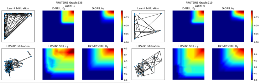
Figure 4: The figure compares the learnt bifiltration function with the Heat-Kernel Signature-Ricci Curvature (HKS-RC) bifiltration on two randomly selected graph instances (838 and 219) of Proteins dataset. These two instances have different labels, 1 and 0 respectively. In the first column, bifiltration function on the vertices of these graphs are plotted. We can see that the learnt bifiltration function is very different from the HKS-RC bifiltration. In the second and third column, Gril vectors are shown using a heatmap for $H_{0}$ and $H_{1}$ respectively. We can observe that these signatures are very different in nature. This provides some evidence that the model is learning a totally different bifiltration function as compared to HKS-RC, which is one of the common choices for bifiltration function on graphs.

Dataset	Num Graphs	Num Classes	Avg. No. Nodes	Avg. No. Edges
Proteins	$1113$	$2$	$39.06$	$72.82$
Cox2	$467$	$2$	$41.22$	$43.45$
Dhfr	$756$	$2$	$42.43$	$44.54$
Mutag	$188$	$2$	$17.93$	$19.79$
Imdb-Binary	$1000$	$2$	$19.77$	$96.53$

Table 5: Description of Benchmark Graph Datasets

Bio-activity Prediction Datasets: The datasets are publicly available in ChEMBL website and can be downloaded following the tutorial mentioned in Sydow et al. (2022). Details about the datasets are given in Table 6. We convert the molecules to graphs with Molfeat. The initial $82$ dimensional node features that is fed to the GNN to get the input bifiltration function are (i) atom-one-hot, (ii) atom-degree-one-hot, (iii) atom-implicit-valence-one-hot, (iv) atom-hybridization-one-hot, (v) atom-is-aromatic, (vi) atom-formal-charge, (vii) atom-num-radical-electrons, (viii) atom-is-in-ring, (ix) atom-total-num-H-one-hot, (x) atom-chiral-tag-one-hot and (xi) atom-is-chiral-center. This is the default setting of Molfeat and we do not claim, in any way, that these are the optimal node features that are to be used.

Dataset	Num Graphs	Active	Inactive	Avg. Num Nodes	Avg. Num Edges
EGFR	4635	2631	2004	28.97	31.73
ERRB2	1818	1140	678	33.33	36.70
CHEMBL1163125	2719	1507	1212	30.77	34.23
CHEMBL203	6816	4234	2582	31.88	34.98
CHEMBL2148	3200	2380	820	29.89	33.28
CHEMBL279	7461	5104	2357	31.82	35.11
CHEMBL2815	3143	2484	659	33.72	37.30
CHEMBL4005	4790	3195	1595	31.79	35.26
CHEMBL4282	3004	2112	892	33.81	37.69
CHEMBL4722	2565	1750	815	31.93	35.29

Table 6: Details of the ChEMBL datasets. Note that compounds with $pIC_{50}>=6.3$ are considered as active molecules.

Experimental Setup:

For the ChEMBL datasets, we used $1$ layer of GIN with a hidden dimension of $64$ to limit the information gained from message passing. The final $3$-layer MLP had hidden dimension of $32$. We ran the experiment for $50$ epochs with an initial learning rate set to be $1e^{-2}$, halved every $10$ epochs. For experiments with additional fingerprints (See Table 2), we used a total of $25$ epochs with an initial learning rate of $1e^{-4}$, halved every $10$ epochs. For all the experiments, we sample every $10$th point in the $100\times 100$ grid resulting in a total of $100$ center points.

References

- Adams et al. (2017) Adams, H., Emerson, T., Kirby, M., Neville, R., Peterson, C., Shipman, P., Chepushtanova, S., Hanson, E., Motta, F., and Ziegelmeier, L. Persistence images: A stable vector representation of persistent homology. Journal of Machine Learning Research, 18(8):1–35, 2017. URL http://jmlr.org/papers/v18/16-337.html.
- Bubenik (2015) Bubenik, P. Statistical topological data analysis using persistence landscapes. J. Mach. Learn. Res., 16:77–102, 2015. doi: 10.5555/2789272.2789275. URL https://dl.acm.org/doi/10.5555/2789272.2789275.
- Burke et al. (2020) Burke, J. V., Curtis, F. E., Lewis, A. S., Overton, M. L., and Simões, L. E. Gradient sampling methods for nonsmooth optimization. Numerical nonsmooth optimization: State of the art algorithms, pp. 201–225, 2020. URL https://link.springer.com/chapter/10.1007/978-3-030-34910-3_6.
- Capecchi et al. (2020) Capecchi, A., Probst, D., and Reymond, J.-L. One molecular fingerprint to rule them all: drugs, biomolecules, and the metabolome. Journal of Cheminformatics, 12(1):43, June 2020. ISSN 1758-2946. doi: 10.1186/s13321-020-00445-4. URL https://jcheminf.biomedcentral.com/articles/10.1186/s13321-020-00445-4.
- Carlsson et al. (2009) Carlsson, G., Singh, G., and Zomorodian, A. Computing multidimensional persistence. In International Symposium on Algorithms and Computation, pp. 730–739. Springer, 2009. URL https://link.springer.com/chapter/10.1007/978-3-642-10631-6_74.
- Carrière & Blumberg (2020) Carrière, M. and Blumberg, A. Multiparameter persistence image for topological machine learning. In Larochelle, H., Ranzato, M., Hadsell, R., Balcan, M., and Lin, H. (eds.), Advances in Neural Information Processing Systems, volume 33, pp. 22432–22444. Curran Associates, Inc., 2020. URL https://proceedings.neurips.cc/paper/2020/file/fdff71fcab656abfbefaabecab1a7f6d-Paper.pdf.
- Carrière et al. (2020) Carrière, M., Chazal, F., Ike, Y., Lacombe, T., Royer, M., and Umeda, Y. Perslay: A neural network layer for persistence diagrams and new graph topological signatures. In Chiappa, S. and Calandra, R. (eds.), Proceedings of the Twenty Third International Conference on Artificial Intelligence and Statistics, volume 108 of Proceedings of Machine Learning Research, pp. 2786–2796. PMLR, 26–28 Aug 2020. URL https://proceedings.mlr.press/v108/carriere20a.html.
- Carrière et al. (2021) Carrière, M., Chazal, F., Glisse, M., Ike, Y., Kannan, H., and Umeda, Y. Optimizing persistent homology based functions. In International conference on machine learning, pp. 1294–1303. PMLR, 2021. URL http://proceedings.mlr.press/v139/carriere21a/carriere21a.pdf.
- Chen & Guestrin (2016) Chen, T. and Guestrin, C. XGBoost: A scalable tree boosting system. In Proceedings of the 22nd ACM SIGKDD International Conference on Knowledge Discovery and Data Mining, KDD ’16, pp. 785–794, New York, NY, USA, 2016. Association for Computing Machinery. ISBN 9781450342322. doi: 10.1145/2939672.2939785. URL https://doi.org/10.1145/2939672.2939785.
- Chen et al. (2023) Chen, Y., Segovia-Dominguez, I., Akcora, C. G., Zhen, Z., Kantarcioglu, M., Gel, Y., and Coskunuzer, B. Emp: Effective multidimensional persistence for graph representation learning. In The Second Learning on Graphs Conference, 2023. URL https://openreview.net/pdf?id=WScCJnX4ek.
- Corbet et al. (2019) Corbet, R., Fugacci, U., Kerber, M., Landi, C., and Wang, B. A kernel for multi-parameter persistent homology. Computers & Graphics: X, 2:100005, 2019. ISSN 2590-1486. doi: https://doi.org/10.1016/j.cagx.2019.100005. URL https://www.sciencedirect.com/science/article/pii/S2590148619300056.
- Davies et al. (2015) Davies, M., Nowotka, M., Papadatos, G., Dedman, N., Gaulton, A., Atkinson, F., Bellis, L., and Overington, J. P. ChEMBL web services: streamlining access to drug discovery data and utilities. Nucleic acids research, 43(W1):W612–W620, 2015. URL https://academic.oup.com/nar/article/43/W1/W612/2467881.
- Davis et al. (2020) Davis, D., Drusvyatskiy, D., Kakade, S., and Lee, J. D. Stochastic subgradient method converges on tame functions. Foundations of computational mathematics, 20(1):119–154, 2020. URL https://link.springer.com/article/10.1007/s10208-018-09409-5.
- Dehmamy et al. (2019) Dehmamy, N., Barabási, A.-L., and Yu, R. Understanding the Representation Power of Graph Neural Networks in Learning Graph Topology. Curran Associates Inc., Red Hook, NY, USA, 2019. URL https://proceedings.neurips.cc/paper/2019/file/73bf6c41e241e28b89d0fb9e0c82f9ce-Paper.pdf.
- Demir et al. (2022) Demir, A., Coskunuzer, B., Gel, Y., Segovia-Dominguez, I., Chen, Y., and Kiziltan, B. Todd: Topological compound fingerprinting in computer-aided drug discovery. Advances in Neural Information Processing Systems, 35:27978–27993, 2022. URL https://openreview.net/pdf?id=8hs7qlWcnGs.
- Dey & Wang (2022) Dey, T. K. and Wang, Y. Computational Topology for Data Analysis. Cambridge University Press, 2022. doi: 10.1017/9781009099950. URL https://www.cs.purdue.edu/homes/tamaldey/book/CTDAbook/CTDAbook.pdf.
- Dey et al. (2024) Dey, T. K., Kim, W., and Mémoli, F. Computing generalized rank invariant for 2-parameter persistence modules via zigzag persistence and its applications. Discret. Comput. Geom., 71(1):67–94, 2024. doi: 10.1007/S00454-023-00584-Z. URL https://doi.org/10.1007/s00454-023-00584-z.
- Edelsbrunner et al. (2002) Edelsbrunner, Letscher, and Zomorodian. Topological persistence and simplification. Discrete & Computational Geometry, 28:511–533, 2002. URL https://link.springer.com/content/pdf/10.1007/s00454-002-2885-2.pdf.
- Edelsbrunner & Harer (2010) Edelsbrunner, H. and Harer, J. Computational Topology: An Introduction. Applied Mathematics. American Mathematical Society, 2010. ISBN 9780821849255.
- Federer (2014) Federer, H. Geometric measure theory. Springer, 2014.
- Gaulton et al. (2012) Gaulton, A., Bellis, L. J., Bento, A. P., Chambers, J., Davies, M., Hersey, A., Light, Y., McGlinchey, S., Michalovich, D., Al-Lazikani, B., et al. ChEMBL: a large-scale bioactivity database for drug discovery. Nucleic acids research, 40(D1):D1100–D1107, 2012. URL https://academic.oup.com/nar/article/40/D1/D1100/2903401?login=false.
- Giunti et al. (2022) Giunti, B., Lazovskis, J., and Rieck, B. Donut: Database of original & non-theoretical uses of topology, 2022. URL https://donut.topology.rocks.
- Goodman & O’Rourke (2004) Goodman, J. E. and O’Rourke, J. Handbook of Discrete and Computational Geometry, Second Edition. Graduate Texts in Mathematics, Vol. 5. CRC Press, Boca Raton, FL, 2004.
- Hofer et al. (2017) Hofer, C. D., Kwitt, R., Niethammer, M., and Uhl, A. Deep learning with topological signatures. In Advances in Neural Information Processing Systems 30: Annual Conference on Neural Information Processing Systems 2017, December 4-9, 2017, Long Beach, CA, USA, pp. 1634–1644, 2017. URL https://proceedings.neurips.cc/paper_files/paper/2017/file/883e881bb4d22a7add958f2d6b052c9f-Paper.pdf.
- Hofer et al. (2019) Hofer, C. D., Kwitt, R., and Niethammer, M. Learning representations of persistence barcodes. J. Mach. Learn. Res., 20(126):1–45, 2019. URL https://www.jmlr.org/papers/volume20/18-358/18-358.pdf.
- Hofer et al. (2020) Hofer, C. D., Graf, F., Rieck, B., Niethammer, M., and Kwitt, R. Graph filtration learning. In Proceedings of the 37th International Conference on Machine Learning, ICML 2020, 13-18 July 2020, Virtual Event, volume 119 of Proceedings of Machine Learning Research, pp. 4314–4323. PMLR, 2020. URL http://proceedings.mlr.press/v119/hofer20b.html.
- Horn et al. (2022) Horn, M., Brouwer, E. D., Moor, M., Moreau, Y., Rieck, B., and Borgwardt, K. M. Topological graph neural networks. In The Tenth International Conference on Learning Representations, ICLR 2022, Virtual Event, April 25-29, 2022. OpenReview.net, 2022. URL https://openreview.net/forum?id=oxxUMeFwEHd.
- Kim et al. (2020) Kim, K., Kim, J., Zaheer, M., Kim, J., Chazal, F., and Wasserman, L. PLLay: Efficient topological layer based on persistent landscapes. In Larochelle, H., Ranzato, M., Hadsell, R., Balcan, M., and Lin, H. (eds.), Advances in Neural Information Processing Systems, volume 33, pp. 15965–15977. Curran Associates, Inc., 2020. URL https://proceedings.neurips.cc/paper/2020/file/b803a9254688e259cde2ec0361c8abe4-Paper.pdf.
- Kim & Mémoli (2021) Kim, W. and Mémoli, F. Generalized persistence diagrams for persistence modules over posets. Journal of Applied and Computational Topology, 5(4):533–581, 12 2021. ISSN 2367-1734. doi: 10.1007/s41468-021-00075-1. URL https://doi.org/10.1007/s41468-021-00075-1.
- Lesnick & Wright (2015) Lesnick, M. and Wright, M. Interactive visualization of 2-d persistence modules. CoRR, abs/1512.00180, 2015. URL http://arxiv.org/abs/1512.00180.
- Leygonie et al. (2021) Leygonie, J., Oudot, S., and Tillmann, U. A framework for differential calculus on persistence barcodes. Foundations of Computational Mathematics, pp. 1–63, 2021. URL https://link.springer.com/article/10.1007/s10208-021-09522-y.
- Loiseaux et al. (2023) Loiseaux, D., Scoccola, L., Carrière, M., Botnan, M. B., and Oudot, S. Stable vectorization of multiparameter persistent homology using signed barcodes as measures. In Thirty-seventh Conference on Neural Information Processing Systems, 2023. URL https://proceedings.neurips.cc/paper_files/paper/2023/hash/d75c474bc01735929a1fab5d0de3b189-Abstract-Conference.html.
- MacLane (1971) MacLane, S. Categories for the working mathematician. Graduate Texts in Mathematics, Vol. 5. Springer-Verlag, New York-Berlin, 1971.
- Morgan (1965) Morgan, H. L. The generation of a unique machine description for chemical structures-a technique developed at chemical abstracts service. Journal of chemical documentation, 5(2):107–113, 1965. URL https://pubs.acs.org/doi/pdf/10.1021/c160017a018.
- Morris et al. (2020) Morris, C., Kriege, N. M., Bause, F., Kersting, K., Mutzel, P., and Neumann, M. TUDataset: A collection of benchmark datasets for learning with graphs. In ICML 2020 Workshop on Graph Representation Learning and Beyond (GRL+ 2020), 2020. URL www.graphlearning.io.
- Noutahi et al. (2023) Noutahi, E., Wognum, C., Mary, H., Hounwanou, H., Kovary, K. M., Gilmour, D., thibaultvarin r, Burns, J., St-Laurent, J., t, DomInvivo, Maheshkar, S., and rbyrne momatx. datamol-io/molfeat: 0.9.4, September 2023. URL https://doi.org/10.5281/zenodo.8373019.
- Reininghaus et al. (2015) Reininghaus, J., Huber, S., Bauer, U., and Kwitt, R. A stable multi-scale kernel for topological machine learning. In Proceedings of the IEEE conference on computer vision and pattern recognition, pp. 4741–4748, 2015. URL https://ieeexplore.ieee.org/abstract/document/7299106.
- Rogers & Hahn (2010) Rogers, D. and Hahn, M. Extended-connectivity fingerprints. Journal of chemical information and modeling, 50(5):742–754, 2010. URL https://pubs.acs.org/doi/abs/10.1021/ci100050t.
- Scoccola et al. (2024) Scoccola, L., Setlur, S., Loiseaux, D., Carrière, M., and Oudot, S. Differentiability and optimization of multiparameter persistent homology. In Forty-first International Conference on Machine Learning, 2024.
- Sydow et al. (2022) Sydow, D., Rodríguez-Guerra, J., Kimber, T. B., Schaller, D., Taylor, C. J., Chen, Y., Leja, M., Misra, S., Wichmann, M., Ariamajd, A., and Volkamer, A. TeachOpenCADD 2022: open source and fair python pipelines to assist in structural bioinformatics and cheminformatics research. Nucleic Acids Research, 50(W1):W753–W760, 2022. URL https://www.ncbi.nlm.nih.gov/pmc/articles/PMC9252772/.
- Van den Dries & Miller (1996) Van den Dries, L. and Miller, C. Geometric categories and o-minimal structures. 1996. URL https://people.math.osu.edu/miller.1987/newg.pdf.
- Vipond (2020) Vipond, O. Multiparameter persistence landscapes. Journal of Machine Learning Research, 21(61):1–38, 2020. URL http://jmlr.org/papers/v21/19-054.html.
- Weininger (1988) Weininger, D. Smiles, a chemical language and information system. 1. introduction to methodology and encoding rules. Journal of chemical information and computer sciences, 28(1):31–36, 1988. URL https://pubs.acs.org/doi/pdf/10.1021/ci00057a005.
- Wilkie (1996) Wilkie, A. Model completeness results for expansions of the ordered field of real numbers by restricted pfaffian functions and the exponential function. Journal of the American Mathematical Society, 9(4):1051–1094, 1996. URL https://community.ams.org/journals/jams/1996-09-04/S0894-0347-96-00216-0/S0894-0347-96-00216-0.pdf.
- Xin et al. (2023) Xin, C., Mukherjee, S., Samaga, S. N., and Dey, T. K. GRIL: a 2-parameter persistence based vectorization for machine learning. In Proceedings of 2nd Annual Workshop on Topology, Algebra, and Geometry in Machine Learning (TAG-ML), volume 221 of Proceedings of Machine Learning Research, pp. 313–333. PMLR, 7 2023. URL https://proceedings.mlr.press/v221/xin23a.html.
- Xu et al. (2019) Xu, K., Hu, W., Leskovec, J., and Jegelka, S. How powerful are graph neural networks? In International Conference on Learning Representations, 2019. URL https://openreview.net/forum?id=ryGs6iA5Km.
- Zomorodian & Carlsson (2004) Zomorodian, A. and Carlsson, G. Computing persistent homology. In Proceedings of the twentieth annual symposium on Computational geometry, pp. 347–356, 2004. URL https://link.springer.com/content/pdf/10.1007/s00454-004-1146-y.pdf.