The Influence of Placement on Transmission in Distributed Computing of Boolean Functions

Abstract

In this paper, we explore a distributed setting, where a user seeks to compute a linearly-separable Boolean function of degree $M$ from $N$ servers, each with a cache size $M$. Exploiting the fundamental concepts of sensitivity and influences of Boolean functions, we devise a novel approach to capture the interplay between dataset placement across servers and server transmissions and to determine the optimal solution for dataset placement that minimizes the communication cost. In particular, we showcase the achievability of the minimum average joint sensitivity, $\frac{N}{2^{M-1}}$, as a measure for the communication cost.

I Introduction

Over the past few decades, technological advancements have significantly increased the demand for high-performance distributed computing to divide a computationally heavy task into multiple subtasks with lower computation load over workers across a network, e.g., machine learning algorithms over distributed servers [1], and cloud computing platforms [2]. Even though there exist heuristic approaches to the problem of distributed computing in the literature, such as MapReduce [3], managing the ever-increasing demands requires a deep understanding of distributed placement, compression, and transmission of datasets towards realizing various computations, which is our key focus in this paper.

I-A Related Work

We first review functional compression literature. We then provide the existing algorithms for distributed placement of datasets to achieve various computation tasks.

From source compression to functional compression

While the fundamental limits for the problem of data compression, either centralized [4] or distributed [5], has been explored, the general problem of compression for computing, or functional compression, requires different tools that can exploit the structure of the computation task. To that end, Körner introduced the notion of graph entropy for distinguishing source symbols that produce different function outcomes [6], and the concept of graph coloring was later used in various distributed functional compression settings, including but not limited to [7, 8, 9]. However, this technique may not apply to general functions. Other works, e.g., [10, 11], to exploit the characteristics of functions, devised structured coding schemes, which require different encoding functions for different tasks and hence may not be practical.

Following the coded distributed computing scheme in [12], several works investigated the storage-computation-communication tradeoffs, e.g., for the class of linearly-separable functions, using cyclic placement [13], or with linear coding for optimizing placement and transmissions [14], using placement delivery arrays [15], and tessellations [16].

The role of placement in distributed computation

The most common placement of datasets across servers in distributed setting’s literature is the “cyclic placement” scheme on datasets, e.g., as in [13]. The placement on distributed servers is conducted in a cyclic manner, in the amount of some circular shifts between two consecutive servers. As a result of cyclic placement, any subset of servers covers the set of all datasets to compute the requested functions from the user.

While the main focus in the related literature is on encoding, transmission, and decoding phases with a given assignment of data, the placement configuration of datasets across servers could significantly affect the communication cost [14, 16].

I-B Motivation and Contributions

Motivated by the impact of dataset placement on transmission in distributed computing systems [14, 16], we utilize the concept of sensitivity and influence of Boolean functions [17], [18] to designate an optimal placement configuration that achieves the minimum communication cost. Specifically, we focus on the linearly-separable Boolean functions.

In this paper, we present a novel distributed computing approach that involves a master node, a set of distributed servers, and a user demanding the error-free computation of a linearly-separable Boolean function. The master node distributes datasets across servers, where each server then performs subcomputations of datasets. Our approach captures the joint influences of subsets of distributed datasets in computing the user demand for any given number of servers with identical cache sizes. This enables us to show the fundamental interplay between the placement and transmission for distributed computation of linearly-separable Boolean functions, where the function structure reveals an optimal placement configuration.

I-C Organization

The rest of the paper is organized as follows. In Section II, we present the proposed scheme for distributed computing of a Boolean function, and the relation between dataset placement and transmissions. Next, in Section III, exploiting the notions of sensitivity and influences of Boolean functions given placement configurations, we propose a novel approach for analyzing the communication cost for distributed computing of linearly separable Boolean functions. Finally, in Section IV, we discuss potential future directions toward extending the influence-based concept to a general class of functions.

Notation. The notation $\mathbb{F}_{2}^{L}$ represents the binary field of length $L$, where $\mathbb{F}_{2}=\{0,1\}$. We use square brackets to represent a set of integers, where $[K]\triangleq\{1,2,\dots,K\}$, given $K\in\mathbb{Z}^{+}$, and curly brackets to denote a set of subsets, e.g., $\{\mathcal{S}_{n}\}$, where $\mathcal{S}_{n}$ is a subset of datasets. For a random variable $X$, $\mathbb{E}[X]$ is its expected value. We denote by $\mathbf{W}=(W_{1},\ldots,W_{K})$ the vector of all datasets. The basis vector notation $e_{k}\triangleq(0,\dots,0,1,0,\dots,0)$ represents a binary vector with cardinality $K$ such that $e_{k}(k)=1$ and $e_{k}(l)=0$, $\forall$ $l\neq k$. The notations $\oplus$ and $\bigoplus$ indicate the modulo two addition and the summation symbol in $\mathbb{F}_{2}$, respectively. Hence, $\mathbf{w}\oplus e_{k}$ represents $\mathbf{w}$ with the $k^{th}$ entry flipped. We denote the indicator function by $1_{\{.\}}$.

II System Model

We consider a distributed computing setup consisting of a master node, a set of distributed servers, and a user. In this setting, there are $K$ independent and identically distributed (i.i.d.) datasets, where each dataset $k\in[K]$ is a Bernoulli distributed random variable, denoted by $W_{k}\sim{\rm Bern}(\frac{1}{2})$. The master node assigns (possibly not disjoint) subsets of datasets $N$ servers indexed by $[N]$, where each server has an identical cache size that allows storing up to $M$ datasets. Finally, the user seeks to compute a Boolean function $f:\mathbb{F}_{2}^{K}\longrightarrow\mathbb{F}_{2}$ of the input vector of all $K$ datasets, i.e., $\mathbf{W}=(W_{1},W_{2},\ldots,W_{k})$.

In this paper, we use the below representation for a Boolean function in general polynomial form [18]:

$$f(\mathbf{W})=\bigoplus_{\mathcal{P}\subseteq[K]}c_{\mathcal{P}}\prod_{k\in\mathcal{P}}W_{k}$$ (1)

for some subsets $\mathcal{P}$ of $K$ datasets and coefficients $c_{\mathcal{P}}\in\mathbb{F}_{2}$.

II-A Phases of Distributed Computing

In this setting, we have three phases for distributed computing of $f(\mathbf{W})$ given the input vector $\mathbf{W}$, as described next.

Dataset Placement

In this phase, the master node will assign a subset of datasets to each server node without coding across different datasets, known as uncoded placement in the literature, see e.g., [19]. In particular, given a cache size of $M$ for each server, the master node will assign subsets of $K$ datasets to the servers according to a placement function $\rho_{n}$, $n\in[N]$ which is described as

$$\rho_{n}:\mathbb{F}_{2}^{K}\longrightarrow\mathbb{F}_{2}^{M}\ ,\quad\forall n\in[N]\ ,$$ (2)

where the assigned subset to the $n^{th}$ server is specified as

$$S_{n}=\rho_{n}(\mathbf{W})\subseteq\{\mathbf{W}\}\ ,\quad|S_{n}|=M\ ,\quad\forall n\in[N]\ .$$ (3)

In other words, the placement phase assigns subsets with a cardinality $M$ of possibly overlapping datasets to the servers. We also denote the set of the assigned subsets, i.e., placement configuration by $\mathcal{S}=\{S_{n}\,|\,n\in[N]\}$.

Encoding and Transmissions

Given the subsets $S_{n},n\in[N]$ from the placement phase, we next detail the encoding phase. Given the subset $S_{n}$ and the computation task $f(\mathbf{W})$, server $n\in[N]$ will conduct subcomputations to determine its transmitted information. Here we note that the servers know the task $f(\mathbf{W})$ a priori and design the subcomputations accordingly. We model the encoding and transmission process at server $n\in[N]$ by the function

$$E_{n}^{f}:\mathbb{F}_{2}^{M}\longrightarrow\mathbb{F}_{2}^{|Z_{n}|}\ ,$$ (4)

where we denote the set of computed data by server $n$ by

$$Z_{n}=E_{n}^{f}(S_{n})=\{Z_{ni}\,|\,i\in[|Z_{n}|]\}\ ,\quad n\in[N]$$ (5)

which is then transmitted to the user. We also denote by $Z=\{Z_{n}\,|\,n\in[N]\}$ the set of all transmitted data by all servers to measure the total number of transmissions. The user, as we describe next, will aggregate the transmissions $Z$ from all servers to determine the output of $f(\mathbf{W})$.

Decoding

We assume that for any given placement configuration and given input vector $\mathbf{W}$, once the user receives the subcomputations from each server, it will be able to calculate the outcome of the Boolean function, i.e., $f(\mathbf{W})$, represented by the general polynomial form in (1). The decoding procedure should be designed based on the placement scheme and the encoding process. The decoding function for the recovery of the function by the user is specified as

$$D:\mathbb{F}_{2}^{|Z|}\longrightarrow\mathbb{F}_{2}\ .$$ (6)

We assume that the user can recover the function without any error. Hence, for error-free recovery of the computation task, the decoding procedure must satisfy $D(Z)=f$.

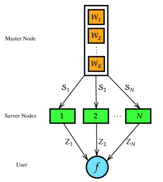
Figure 1: A generic distributed computing system model.

We illustrate the system model for our distributed computing scheme in Figure 1. In this work, we focus on linearly-separable Boolean function of degree $d$ as

$$f(\mathbf{W})=\bigoplus_{n=1}^{N}f_{n}\ ,$$

$$f_{n}=\underset{k\in\mathcal{K}_{\mathcal{P}_{n},d}}{\prod}W_{k}\ ,$$ (7)

where $\mathcal{K}_{\mathcal{P},d}$ is a subset $\mathcal{P}$ with cardinality $d$ of $K$ datasets:

$$\mathcal{K}_{\mathcal{P},d}\triangleq\{\mathcal{P}\subseteq{[K]}\ |\ |\mathcal{P}|=d\}\ ,$$ (8)

where $d=M$. We also assume that $K=NM$, implying $N$ servers each with cache size $M$.

We refer to our system model as a $(K,N,M,\mathcal{S},f)$ distributed computing scheme. We next define an achievable scheme for error-free distributed computing of $f$ at the user.

Definition 1.

(An achievable distributed computing scheme.) A $(K,N,M,\mathcal{S},f)$ distributed computing scheme is called achievable if the function $f$ can be recovered in an error-free manner by the user with the given cache configuration, i.e., $D(Z)=f$, where $Z$ is possibly a nonlinear combination of the encoded data $Z_{n}=E_{n}^{f}(\mathcal{S}_{n})$, $n\in[N]$, which is placement-dependent and function-aware.

Exploiting the definition of $Z=\{Z_{n}\,|\,n\in[N]\}$, we denote the total number of transmissions by all servers as

$$T^{(\mathcal{S})}\triangleq|Z|=\sum_{n=1}^{N}|Z_{n}|\ .$$ (9)

We next consider an example to demonstrate the interplay between the placement configuration and the value of $T^{(\mathcal{S})}$ for the given $(K,N,M,\mathcal{S},f)$ distributed computing scheme. We will then show the connection between our model for communication cost and $T^{(\mathcal{S})}$ in Section III.

II-B The Interplay between Placement and Transmission

In this subsection, we first present an example, with two different placement configurations, namely $\mathcal{S}^{(1)}$ which is cyclic, and $\mathcal{S}^{(2)}$, for computing a Boolean function. We next contrast the total number of transmissions needed in each configuration to demonstrate the role of placement and transmissions.

Example 1.

Consider a $(K=9,\ N=3,\ M=6,\ \mathcal{S},\ f)$ distributed computing system, where

$$f(\mathbf{W})=W_{1}W_{4}W_{7}\oplus W_{2}W_{5}W_{8}W_{7}\oplus W_{3}W_{6}W_{9}\ .$$ (10)

1. Configuration $\mathcal{S}^{(1)}:$ The dataset assignment is cyclic such that $\mathcal{S}^{(1)}_{1}=\{W_{1},W_{2},W_{3},W_{4},W_{5},W_{6}\}$, $\mathcal{S}^{(1)}_{2}=\{W_{4},W_{5},W_{6},W_{7},W_{8},W_{9}\}$, and $\mathcal{S}^{(1)}_{3}=\{W_{1},W_{2},W_{3},W_{7},W_{8},W_{9}\}$, satisfying the cache size constraint with equality. To successfully compute (10) in this configuration, it suffices that the servers need to compute and transmit data as shown in Table I. Hence, this scenario requires $T^{\mathcal{S}^{(1)}}=6$ transmissions in total.

   Assigned subsets	Transmitted data
   $S_{1}^{(1)}$	$Z_{11}^{(1)}=W_{1}W_{4}$, $Z_{12}^{(1)}=W_{3}W_{6}$, $Z_{13}^{(1)}=W_{2}$
   $S_{2}^{(1)}$	$Z_{21}^{(1)}=W_{5}W_{8}W_{7}$, $Z_{22}^{(1)}=W_{7}$, $Z_{23}^{(1)}=W_{9}$
   $S_{3}^{(1)}$	No transmissions

   TABLE I: Server-transmission details for $\mathcal{S}^{(1)}$.

2. Configuration $\mathcal{S}^{(2)}:$ The dataset assignment satisfies $\mathcal{S}^{(2)}_{1}=\{W_{1},W_{2},W_{4},W_{5},W_{6},W_{7}\}$, $\mathcal{S}^{(2)}_{2}=\{W_{3},W_{4},W_{5},W_{6},W_{8},W_{9}\}$, and $\mathcal{S}^{(2)}_{3}=\{W_{1},W_{2},W_{3},W_{7},W_{8},W_{9}\}$. To successfully compute (10) in this setting, without the presence of stragglers, a viable transmission scheme is shown in Table II. Thanks to a better arrangement of the datasets that is sensitive to the function in $\mathcal{S}^{(2)}$ versus $\mathcal{S}^{(1)}$, the total number of transmissions is $T^{\mathcal{S}^{(2)}}=4<T^{\mathcal{S}^{(1)}}=6$.

   Assigned subsets	Transmitted data
   $S_{1}^{(2)}$	$Z_{11}^{(2)}=W_{1}W_{4}W_{7}$, $Z_{12}^{(2)}=W_{2}W_{5}W_{7}$
   $S_{2}^{(2)}$	$Z_{21}^{(2)}=W_{3}W_{6}W_{9}$, $Z_{22}^{(2)}=W_{8}$
   $S_{3}^{(2)}$	No transmissions

   TABLE II: Server-transmission details for $\mathcal{S}^{(2)}$.

We infer from Example 1 how a cleverly conducted placement phase in distributed computing settings could dramatically reduce the total number of transmissions needed for error-free recovery of the Boolean function at the user.

To evaluate the communication cost of the $(K,N,M,\mathcal{S},f)$ distributed computing scheme, we will next detail a novel approach that relies on the average joint sensitivity of the computation task abstracted by the Boolean function.

III Main Results

In this section, to determine the role of the placement configuration on the communication cost, we first provide a primer on the sensitivity of a Boolean function on its input, and the influence of a set of input variables on the outcome of the function. We then present our main results.

III-A Joint Sensitivity and Influences

Building on the classical notions of sensitivity, influence, and average sensitivity tailored for capturing the sensitivity of a Boolean function by modifying one dataset at each time [17, 18], we will exploit the joint behavior of datasets across servers, as in [20]. A Boolean function $f(\mathbf{W})$ depends on its $k^{th}$ input variable if there exists at least one $\mathbf{W}\in\mathbb{F}_{2}^{K}$ such that $f(\mathbf{W}\oplus e_{k})\neq f(\mathbf{W})$. To that end, we next define the sensitivity of $f(\mathbf{W})$ on a set of $W_{k}$’s.

Definition 2.

(Joint sensitivity.) The joint sensitivity of $f(\mathbf{W})$ to the set $\mathcal{S}$ of subsets of datasets is defined as

$${\rm Sen}_{\mathcal{S}}(f,\mathbf{W})=\sum\limits_{n=1}^{|\mathcal{S}|}{\rm Sen}_{\mathcal{S}_{n}}(f,\mathbf{W})\ ,$$ (11)

where $e_{\mathcal{S}_{n}}\triangleq\underset{\{k|w_{k}\in\mathcal{S}_{n}\}}{\bigoplus}e_{k}$ describes the multi-dataset flipped vector, the measure ${\rm Sen}_{\mathcal{S}_{n}}(f,\mathbf{W})=1_{f(\mathbf{W}\oplus e_{\mathcal{S}_{n}})\neq f(\mathbf{W})}$ captures the sensitivity of $f(\mathbf{W})$ on input $\mathbf{W}$ with the jointly flipped entry datasets with indices $k$ such that $W_{k}\in\mathcal{S}_{n}\subseteq\mathcal{S}$.

Definition 3.

(Joint influence.) The joint influence of the datasets of $\mathcal{S}_{n}$ on the function $f$ is defined as

$${\rm Inf}_{\mathcal{S}_{n}}(f) =\mathbb{P}[f(\mathbf{W}\oplus e_{\mathcal{S}_{n}})\neq f(\mathbf{W})]$$

$$=\mathbb{E}_{\mathbf{W}}[{\rm Sen}_{\mathcal{S}_{n}}(f,\mathbf{W})]\ .$$ (12)

Definitions 2-3 allow us to introduce our next key metric.

Definition 4.

(Average joint sensitivity.) The average joint sensitivity of $f(\mathbf{W})$ to the set $\mathcal{S}=\{S_{n}|n\in[N]\}$ of all possible datasets specified by $\rho_{n}$ given a cache size constraint $M$ is given as follows:

$${\rm as_{\mathcal{S}}}(f) =\mathbb{E}_{\mathbf{W}}[{\rm Sen}_{\mathcal{S}}(f,\mathbf{W})]$$

$$=\sum\limits_{n=1}^{|\mathcal{S}|}{\rm Inf}_{\mathcal{S}_{n}}(f)\ .$$ (13)

Utilizing Definitions 2-4, we can next present our approach for formulating an optimal dataset placement configuration from a communication cost perspective.

III-B The Communication-Optimal Placement Configuration

To evaluate the tradeoff between placement and communication cost for computing a Boolean function $f$, we first present a Lemma that focuses on each product subfunction $f_{n}$ given in (II-A) to obtain the joint influence of datasets on $f_{n}$.

Lemma 1.

(Joint influence on a product subfunction.) The joint influence of multiple datasets in a subset $\mathcal{S}_{n}$ with an arbitrary size from a product subfunction $f_{n}(\mathbf{W})=\underset{{k\in\mathcal{K}_{\mathcal{P},d}}}{\prod}W_{k}$ of degree $d$ equals the influence of each dataset on $f_{n}$, i.e.,

$${\rm Inf}_{\mathcal{S}_{n}}(f)={\rm Inf}_{k}(f)=\frac{1}{2^{d-1}}\ .$$ (14)

Proof.

See Appendix -A. ∎

Towards determining the joint influence of datasets on $f$ in (II-A), we next present another Lemma that contrasts the joint influence of datasets for the summation of two product subfunctions, namely $f_{n}$ and $f_{n^{\prime}}$ where $n^{\prime}\neq n$, for different dataset placement configurations. To that end, we denote the set of variables included in the subfunction $f_{n}$ as

$$\mathcal{I}_{f_{n}}\triangleq\{W_{k}\,|\,f_{n}=\underset{k\in\mathcal{K}_{\mathcal{P}_{n},d}}{\prod}W_{k}\},\quad\forall n\in[N]\ .$$ (15)

Lemma 2.

(Increase in joint influence due to summation.) Let $f=f_{n}\oplus f_{n^{\prime}}$, where $n\neq n^{\prime}$. Consider two different subsets of datasets denoted by $\mathcal{S}_{1}=\{W_{k}|W_{k}\in\mathcal{I}_{f_{n}}\}$ and $\mathcal{S}^{\prime}_{1}=\{W_{k}|W_{k}\in\mathcal{I}_{f_{n}}\cup\mathcal{I}_{f_{n^{\prime}}}\}$. We then have:

$${\rm Inf}_{\mathcal{S}^{\prime}_{1}}(f)\geq{\rm Inf}_{\mathcal{S}_{1}}(f)\ .$$ (16)

Proof.

See Appendix -B. ∎

From Lemma 2, the subsets with the lowest joint influence include datasets from the same $f_{n}$. We next derive a lower bound on the average joint sensitivity for the proposed setting using Lemmas 1-2, and present the communication-optimal placement configuration in Theorem 1.

Theorem 1.

(A communication-optimal placement configuration.) Given a $(K,N,M,\mathcal{S},f)$ distributed computing scheme, the average joint sensitivity and the total number of transmissions are lower bounded by

$${\rm as_{\mathcal{S}}}(f)\geq{\rm as_{\mathcal{S}^{*}}}(f)=\frac{N}{2^{M-1}}\ ,$$

$$T^{(\mathcal{S})}\geq T^{(\mathcal{S}^{*})}=N\ ,$$ (17)

respectively, corresponding to $\mathcal{S}^{*}=\{\mathcal{S}^{*}_{n}\,|\,n\in[N]\}$, where $\mathcal{S}^{*}_{n}=\{W_{k}\,|\,W_{k}\in\mathcal{I}_{f_{n}}\}$.

Proof.

See Appendix -C. ∎

Corollary 1.

The number of transmissions by server $n$ is a monotonically increasing function in terms of the joint influence of datasets in each subset on Boolean function $f$, i.e., $|Z_{n}|\leq|Z_{n^{\prime}}|$ if and only if ${\rm Inf}_{\mathcal{S}_{n}}(f)\leq{\rm Inf}_{\mathcal{S}_{n^{\prime}}}(f),\,\forall n\neq n^{\prime}$.

From Corollary 1, it is easy to observe that $T^{(\mathcal{S})}$ is a monotonically increasing function of the average joint sensitivity, i.e., $T^{(\mathcal{S})}\leq T^{(\mathcal{S}^{\prime})}$ if and only if ${\rm as}_{\mathcal{S}}(f)\leq{\rm as}_{\mathcal{S}^{\prime}}(f)$.

IV Conclusions

In this work, using the concept of sensitivity and influence, we introduced a novel approach for determining the interplay between communication cost and placement configuration for distributed computing of Boolean functions. In particular, we specified the optimal placement configuration from a communication cost perspective for a class of linearly-separable Boolean functions. Our approach is based on grouping the datasets to minimize the summation of their joint influences. As a future direction, we will extend our approach to distributed computing of nonlinear Boolean functions.

-A Proof of Lemma 1

Using Definition 3 and its probabilistic nature, we have:

$${\rm Inf}_{\mathcal{S}_{n}}(f) =\mathbb{P}\Big{[}f(\mathbf{W}\oplus e_{\mathcal{S}_{n}})\neq f(\mathbf{W})\Big{]}$$

$$\overset{(*)}{=}\frac{2}{2^{d}}=\frac{1}{2^{d-1}}\ ,$$

where $(*)$ holds since only two sequences $11\ldots 1$ and $00\ldots 0$ out of $2^{d}$ possible sequences are feasible. Similarly, for the individual variable $W_{k}$, the influence is calculated as

$${\rm Inf}_{k}(f)=\mathbb{P}\Big{[}\underset{i\in\mathcal{K}_{\mathcal{P}\backslash k,d-1}}{\prod}W_{i}\neq 0\Big{]}=\Big{(}\frac{1}{2}\Big{)}^{d-1}\ ,$$ (18)

where the last step follows when all the $d-1$ datasets $W_{k}\sim{\rm Bern}(\frac{1}{2})$, $k\in\mathcal{K}_{\mathcal{P}\backslash k,d-1}$ are equal to $1$. Therefore, (14) holds.

-B Proof of Lemma 2

According to Lemma 1, ${\rm Inf}_{\mathcal{S}_{1}}(f)=\frac{1}{2^{d-1}}$. To find the joint influence of subset $\mathcal{S}^{\prime}_{1}$ on $f=f_{n}\oplus f_{n^{\prime}}$, we first consider only one dataset difference between $\mathcal{S}_{1}$ and $\mathcal{S}^{\prime}_{1}$, i.e., we assume $\mathcal{S}^{\prime}_{1}=\{W_{k}|W_{k}\in\mathcal{I}_{f_{n}}\backslash W_{n}\cup W_{n^{\prime}}\}$. We then decompose the respective product subfunctions as

$$f_{j}=\underset{k\in\mathcal{K}_{\mathcal{P}_{j}\backslash j,d-1}}{\prod}W_{k}W_{j}\ ,\quad j\in\{n,\,n^{\prime}\}\ .$$

Using Definition 3, we can rewrite ${\rm Inf}_{\mathcal{S}^{\prime}_{1}}(f)$ as

$${\rm Inf}_{\mathcal{S}^{\prime}_{1}}(f) =\mathbb{P}[\underset{k\in\mathcal{K}_{\mathcal{P}_{n}\backslash n,d-1}}{\prod}(W_{k}\oplus 1)W_{n}$$

$$\oplus\underset{k\in\mathcal{K}_{\mathcal{P}_{n^{\prime}}\backslash n^{\prime},d-1}}{\prod}W_{k}(W_{n^{\prime}}\oplus 1)$$

$$\neq\underset{k\in\mathcal{K}_{\mathcal{P}_{n}\backslash n,d-1}}{\prod}W_{k}W_{n}\oplus\underset{k\in\mathcal{K}_{\mathcal{P}_{n^{\prime}}\backslash n^{\prime},d-1}}{\prod}W_{k}W_{n^{\prime}}]$$

$$=\mathbb{P}\Big{[}\bigoplus_{i=0}^{d-2}\underset{k\in\mathcal{K}_{\mathcal{P}_{n}\backslash n,i}}{\prod}W_{k}W_{n}\oplus\underset{k\in\mathcal{K}_{\mathcal{P}_{n^{\prime}}\backslash n^{\prime},d-1}}{\prod}W_{k}\neq 0\Big{]}\ .$$ (19)

Let $\Delta f\triangleq\bigoplus_{i=0}^{d-2}\underset{k\in\mathcal{K}_{\mathcal{P}_{n}\backslash n,i}}{\prod}W_{k}W_{n}\oplus\underset{k\in\mathcal{K}_{\mathcal{P}_{n^{\prime}}\backslash n^{\prime},d-1}}{\prod}W_{k}$. Considering the law of total probability and i.i.d. datasets:

$$\mathbb{P}[\Delta f=1] =\frac{1}{2}\left(\mathbb{P}[\Delta f=1\,|\,W_{n}=1]\right.$$

$$\left.+\mathbb{P}[\Delta f=1\,|\,W_{n}=0]\right)\ ,$$

where using Lemma 1, we obtain:

$$\mathbb{P}[\Delta f=1\,|\,W_{n}=0] =\mathbb{P}[\underset{k\in\mathcal{K}_{\mathcal{P}_{n^{\prime}}\backslash n^{\prime},d-1}}{\prod}W_{k}=1]$$

$$=\Big{(}\frac{1}{2}\Big{)}^{d-1}\ ,$$

$$\mathbb{P}[\Delta f=1\,|\,W_{n}=1]$$

$$=\mathbb{P}\Big{[}\bigoplus_{i=0}^{d-2}\underset{k\in\mathcal{K}_{\mathcal{P}_{n}\backslash n,i}}{\prod}W_{k}\oplus\underset{k\in\mathcal{K}_{\mathcal{P}_{n^{\prime}}\backslash n^{\prime},d-1}}{\prod}W_{k}=1\Big{]}$$

$$=\mathbb{P}\Big{[}\bigoplus_{i=0}^{d-2}\underset{k\in\mathcal{K}_{\mathcal{P}_{n}\backslash n,i}}{\prod}W_{k}=0,\underset{k\in\mathcal{K}_{\mathcal{P}_{n^{\prime}}\backslash n^{\prime},d-1}}{\prod}W_{k}=1\Big{]}$$

$$+\mathbb{P}\Big{[}\bigoplus_{i=0}^{d-2}\underset{k\in\mathcal{K}_{\mathcal{P}_{n}\backslash n,i}}{\prod}W_{k}=1,\underset{k\in\mathcal{K}_{\mathcal{P}_{n^{\prime}}\backslash n^{\prime},d-1}}{\prod}W_{k}=0\Big{]}$$

$$=\Big{[}1-\Big{(}\frac{1}{2}\Big{)}^{d-2}\Big{]}\Big{(}\frac{1}{2}\Big{)}^{d-1}+\Big{(}\frac{1}{2}\Big{)}^{d-2}\Big{[}1-\Big{(}\frac{1}{2}\Big{)}^{d-1}\Big{]}\ .$$ (20)

After rearranging (-B) and applying it to (-B), we obtain:

$${\rm Inf}_{\mathcal{S}^{\prime}_{1}}(f)=2\Big{(}\frac{1}{2}\Big{)}^{d-1}\Big{[}1-\Big{(}\frac{1}{2}\Big{)}^{d-1}\Big{]}\ .$$ (21)

It is obvious that ${\rm Inf}_{\mathcal{S}^{\prime}_{1}}(f)\geq(\frac{1}{2})^{d-1}={\rm Inf}_{\mathcal{S}_{1}}(f)$. By induction, it follows that for any subset $\mathcal{S}^{\prime}_{1}$ with more difference than one dataset compared to $\mathcal{S}_{1}$, (16) holds.

-C Proof of Theorem 1

We prove this theorem in two parts:

Achievability

For distributed computing of a linearly-separable Boolean function $f$ of degree $M$, there exists an achievable scheme with a placement configuration $\mathcal{S}^{*}$.

According to Lemma 1, ${\rm Inf_{\mathcal{S}_{n}^{*}}}(f)=\frac{1}{2^{M-1}},\forall n\in[N]$. The average joint sensitivity in this case is therefore:

$${\rm as_{\mathcal{S}^{*}}}(f) =\sum_{n=1}^{N}\frac{1}{2^{M-1}}$$

$$=\frac{N}{2^{M-1}}\ .$$ (22)

According to Definition 1, the $(K,N,M,\mathcal{S}^{*},f)$ distributed computing scheme is achievable since the user with cache configuration $\mathcal{S}^{*}$ would be able to recover the function in an error-free manner with only summing $Z^{*}_{n}$’s together, i.e.,

$$D(Z^{*}) =\bigoplus_{n=1}^{N}Z^{*}_{n}$$

$$=\bigoplus_{n=1}^{N}\underset{k\in\mathcal{K}_{\mathcal{P}^{*}_{n},M}}{\prod}W_{k}$$

$$=\bigoplus_{n=1}^{N}f_{n}=f\ .$$ (23)

Optimality (converse)

Based on Lemma 2, the minimum joint influence happens when we group the datasets from the same product subfunction. We then use it to show the optimality of our proposed placement configuration.

We then examine a placement scheme $\mathcal{S}$, where we consider similar placement as $\mathcal{S}^{*}$ for $N-2$ servers. For simplicity, we only swap two datasets between the two first servers. They will therefore contain subsets $\mathcal{S}_{1}=\{W_{k}\,|\,W_{k}\in\mathcal{I}_{f_{n}}\backslash W_{n}\cup W_{n^{\prime}}\}$ and $\mathcal{S}_{2}=\{W_{k}\,|\,W_{k}\in\mathcal{I}_{f_{n^{\prime}}}\backslash W_{n^{\prime}}\cup W_{n}\}$, respectively. In other words, we group $M-1$ datasets from $\mathcal{I}_{f_{n}}$ and one variable ($W_{n^{\prime}}$) from $\mathcal{I}_{f_{n^{\prime}}}$ in $\mathcal{S}_{1}$ and vice versa in $\mathcal{S}_{2}$. According to Lemma 1 and Lemma 2, we have:

$${\rm Inf}_{\mathcal{S}_{n}}(f)\geq{\rm Inf}_{\mathcal{S}^{*}_{n}}(f)=\frac{1}{2^{M-1}},\ \forall n=1,2\ .$$ (24)

For other $N-2$ subsets, we also have:

$${\rm Inf}_{\mathcal{S}_{n}}(f)={\rm Inf}_{\mathcal{S}^{*}_{n}}(f)=\frac{1}{2^{M-1}}\ .$$ (25)

Using Definition 4 and summing the joint influences together for both $\mathcal{S}$ and $\mathcal{S}^{*}$ completes the proof. By induction, it follows that for any placement configuration $\mathcal{S}$ with more swapped datasets between subsets compared to $\mathcal{S}^{*}$, (1) holds. We also note that the minimum value of $T^{(\mathcal{S})}$ corresponds to $\mathcal{S}^{*}$ and equals to $N$, i.e., the transmission of $N$ units of data.

References

• [1] H. Li, Y. Chen, K. W. Shum, and C. W. Sung, “Data allocation for approximate gradient coding in edge networks,” in Proc., IEEE ISIT, Taipei, Taiwan, 2023, pp. 2541–2546.
• [2] X. Xu, M. Tang, and Y.-C. Tian, “Theoretical results of QoS-guaranteed resource scaling for cloud-based MapReduce,” IEEE Trans. Cloud Comput., vol. 6, no. 3, pp. 879–889, 2018.
• [3] J. Dean and S. Ghemawat, “MapReduce: Simplified data processing on large clusters,” Commun. ACM, vol. 51, no. 1, p. 107–113, Jan. 2008.
• [4] C. E. Shannon, “A mathematical theory of communication,” Bell Syst. Tech. J., vol. 27, no. 3, pp. 379–423, Jul. 1948.
• [5] D. Slepian and J. Wolf, “Noiseless coding of correlated information sources,” IEEE Trans. Inf. Theory, vol. 19, no. 4, pp. 471–480, 1973.
• [6] J. Körner, “Coding of an information source having ambiguous alphabet and the entropy of graphs,” in Proc., 6th Prague Conf. Inf. Theory, Prague, Czech Republic, Sep. 1973, pp. 411–425.
• [7] A. Orlitsky and J. R. Roche, “Coding for computing,” IEEE Trans. Inf. Theory, vol. 47, no. 3, pp. 903–17, Mar. 2001.
• [8] S. Feizi and M. Médard, “On network functional compression,” IEEE Trans. Inf. Theory, vol. 60, no. 9, pp. 5387–5401, Jun. 2014.
• [9] D. Malak, “Distributed computing of functions of structured sources with helper side information,” in Proc., IEEE SPAWC, Shanghai, China, Sep. 2023, pp. 276–280.
• [10] J. Körner and K. Marton, “How to encode the modulo-two sum of binary sources (corresp.),” IEEE Trans. Inf. Theory, vol. 25, no. 2, pp. 219–221, Mar. 1979.
• [11] T. Han and K. Kobayashi, “A dichotomy of functions F (X, Y) of correlated sources (X, Y),” IEEE Trans. Inf. Theory, vol. 33, no. 1, pp. 69–76, Jan. 1987.
• [12] S. Li, M. A. Maddah-Ali, Q. Yu, and A. S. Avestimehr, “A fundamental tradeoff between computation and communication in distributed computing,” IEEE Trans. Inf. Theory, vol. 64, no. 1, pp. 109–128, 2018.
• [13] K. Wan, H. Sun, M. Ji, and G. Caire, “Distributed linearly separable computation,” IEEE Trans. Inf. Theory, vol. 68, no. 2, pp. 1259–1278, Feb. 2022.
• [14] A. Khalesi and P. Elia, “Multi-user linearly-separable distributed computing,” IEEE Trans. Inf. Theory, vol. 69, no. 10, pp. 6314–6339, 2023.
• [15] Q. Yan, S. Yang, and M. Wigger, “Storage-computation-communication tradeoff in distributed computing: Fundamental limits and complexity,” IEEE Trans. Inf. Theory, vol. 68, no. 8, pp. 5496–5512, 2022.
• [16] A. Khalesi and P. Elia, “Tessellated distributed computing,” 2024. [Online]. Available: https://arxiv.org/abs/2404.14203
• [17] J. Bourgain, J. Kahn, G. Kalai, and et. al., “The influence of variables in product spaces,” Isr. J. Math., vol. 77, pp. 55–64, 1992.
• [18] S. Jukna, Boolean function complexity: advances and frontiers.   Springer, 2012, vol. 5.
• [19] S. Jin, Y. Cui, H. Liu, and G. Caire, “Uncoded placement optimization for coded delivery,” in Proc., IEEE WiOpt, Shanghai, China, May 2018.
• [20] A. Biswas and P. Sarkar, “Influence of a set of variables on a Boolean function,” SIAM J. Discrete Math., vol. 37, no. 3, pp. 2148–2171, 2023.