Constraining $\nu$SMEFT coefficients: the case of the extra $\text{U}(1)^{\prime}$

Abstract

We study the constraints on low-energy coefficients of the $\nu$SMEFT generalization of the Standard Model effective theory in the simple case of a $\text{U}(1)^{\prime}$ enlargement of the Standard Model gauge group. In particular, we analyse the constraints imposed by the requirement that the extended theory remains free of gauge anomalies. We present the cases of explicit realisations, showing the obtained correlations among the coefficients of $d=6$ operators.

I Introduction

The search for physics beyond the Standard Model (SM) is justified by several motivations. There are conceptual issues and cosmological observations suggesting the existence of a more fundamental theory beyond SM. Tensions between SM predictions and experimental results, in particular in the flavour sector, reinforce such a widespread conviction. However, direct searches at colliders have not produced evidence of new particles and/or mediators of new interactions, yet, hence the alternative way to gain evidence of physics beyond the Standard Model (BSM) is investigating virtual effects of possible new heavy degrees of freedom, as done in flavour physics [1].

In this framework, two approaches can be followed towards BSM. The first one consists in formulating a specific extended theory and deriving predictions to be contrasted with experiment for a validation or a discrimination with respect to different new physics (NP) scenarios. The second approach consists in extending the SM at the electroweak (EW) scale in the most general way compatible with the SM gauge symmetry, investigating the constraints imposed by the experiments on the resulting generalization.

A remarkable example of the second approach is the Standard Model effective field theory (SMEFT) [2, 3, 4, 5], widely used in the quest for BSM physics. The SM is considered as an effective field theory describing physics at and below the EW scale. At higher scales a new gauge theory (the UV completion) should exist, with a gauge group extending the SM one and undergoing spontaneous symmetry breaking (SSB) to it. If $\Lambda$ is the NP scale, at the EW scale the SMEFT Lagrangian consists of an expansion in the small parameter $v/\Lambda$, with $v$ the SM Higgs vacuum expectation value. The first term of the expansion is the SM Lagrangian density containing operators of canonical dimension up to $d=4$. Subsequent terms are suppressed by powers of $v/\Lambda$ and comprise operators of increasing dimension:

$${\cal L}_{\rm SMEFT}={\cal L}_{\rm SM}^{(4)}+{\cal L}^{(5)}+{\cal L}^{(6)}+\dots\;.$$ (1)

The apex $(d)$ indicates the canonical dimension of the operators entering in each term ${\cal L}^{(d)}$ written as

$${\cal L}^{(d)}=\sum_{i}\frac{C_{i}}{\Lambda^{d-4}}\,{\cal O}_{i}^{(d)}\;,$$ (2)

with dimensionless Wilson coefficients $C_{i}$. The operators are constructed in terms of the SM fields and satisfy the SM gauge symmetry. SM accidental symmetries are allowed to be violated: for example, baryon and lepton number violating operators are included in (2), namely odd-dimension operators violating $B$ and/or $L$ conservation [6]. The operators contain no reference to the field content of the UV theory. However, their coefficients depend of the details of such a theory, i.e. the couplings and masses of the new particles that, supposed to be $M\simeq{\cal O}(\Lambda)$, are integrated out in the effective field theory (EFT) Lagrangian at the EW scale. A few assumptions concern the UV theory. It should contain only particles with spin $J\leq 1$; new vector fields could be either gauge fields (massless before SSB in the UV theory) or massive Proca fields; new fermions can be introduced provided that they are vector-like with respect to the SM gauge group, to maintain the SM free of gauge anomalies.

One can use the construction in two ways. Choosing the UV completion, the Wilson coefficients of the SMEFT operators can be determined through matching and running procedure [7, 8, 9]. On the other hand, without assumptions on the UV completion, the coefficients are treated as parameters. These two steps are complementary to each other. Having gained model independent information on the coefficients in the effective theory, it is possible to contrast them with the features required in a specific scenario in order to validate or discard it.

The phenomenological evidence that neutrinos have nonvanishing mass induces to consider the $\nu$SMEFT extension of SMEFT, which comprises three right-handed sterile neutrino fields in the sub-TeV mass range [10, 11, 12, 13, 14, 15]. The inclusion does not invalidate the requirement that the SM gauge group is free of gauge anomalies. In the extension, ${\cal L}^{(5)}$ consists of three operators, while only the Weinberg operator appears at this order in the absence of $\nu_{R}$ [16]. The choice of the $d=6$ operators is not unique, and different bases have been proposed, i.e. complete sets of independent, non redundant operators.​​​​ A popular basis is the Warsaw one [3]. In each basis the operators are collected in classes according to their field content.

In our study we focus on the UV completion represented by the simplest extension of the SM gauge group comprising a new $\text{U}(1)^{\prime}$ gauge group, featured by the gauge coupling $g_{Z}$ [17, 18, 19, 20]. $Z^{\prime}$ is the corresponding gauge field, and the $z$-hypercharge is the quantum number associated to the new symmetry. Many NP models introduce such a mediator with specific $z$-hypercharge assignments. Experimental searches for $Z^{\prime}$ rely on the assumptions for the hypercharges, and produce exclusion plots in the plane of the $Z^{\prime}$ production cross section versus $M_{Z^{\prime}}$. ​​​​​​ The NP scale can be identified with $M_{Z^{\prime}}$ acquired after spontaneous breaking of the new symmetry. We do not need to specify how such SSB occurs, we only assume that it happens at a much higher scale than the SM Higgs vev. We neglect the mixing with other neutral gauge bosons.​​​

In the chosen extension we work out the coefficients of the $\nu$SMEFT operators of dimension up to $d=6$, aiming at the relations among them.​​​​ While the gauge structure of the theory already imposes nontrivial relations among various coefficients, further relations can be established requiring that the extended gauge group is anomaly free. We obtain results holding for a generic $\text{U}(1)^{\prime}$ extension. We also consider specific cases: universal $Z^{\prime}$ couplings to the three generations or only to the third generation; $Z^{\prime}$ only coupled to left- or right-handed fermions; lepto- or hadrophobic $Z^{\prime}$; the $z$-hypercharge assignment of the ABCD model [23]. In all cases, we find that the number of independent coefficients is reduced and remarkable correlations can be established among them, which are peculiar of each extension. The experimental test of such correlations would shed light on the particular completion, providing the widest information using measurements.

The plan of the paper is as follows. After Sec. II with the notations, in Sec. III we list the $\nu$SMEFT operators generated at the EW scale when the UV theory contains the new gauge boson $Z^{\prime}$. The impact of the new gauge boson on the SMEFT Lagrangian density is considered in Sec. IV, with the list of the operators obtained when the $Z^{\prime}$ field is integrated out, the expressions of their Wilson coefficients and the relations due to the gauge structure of the extension. In Sec. V we consider the relations that the fermion $z$-hypercharges must satisfy to fulfil the requirement of gauge anomaly cancellation in the SM gauge group extension, and how such relations can be translated into analogous ones among the SMEFT coefficients. We than discuss the results for the selected $z$-hypercharge assignments. The last section comprises the conclusions.

II Notations, $Z^{\prime}$ couplings to fermions and to the Higgs field

We denote by $q_{L}^{i}$ and $\ell_{L}^{i}$ the $\text{SU}(2)_{L}$ left-handed quark and lepton doublets, respectively, with generation index $i=\{1,2,3\}$. $u_{R}^{i},\,d_{R}^{i},\,\nu_{R}^{i},\,e_{R}^{i}$ are right-handed singlets.

Before the electroweak SSB the $Z^{\prime}$ couplings to fermions are flavour conserving, hence for a generic fermion $\psi$ we can write

$${\cal L}_{\rm int}^{Z^{\prime}}=g_{Z}\,z_{\psi}\,\bar{\psi}\,\gamma^{\mu}\,\psi\,Z_{\mu}^{\prime}\;.$$ (3)

$Z_{\mu}^{\prime}$ is the gauge boson field, $g_{Z}$ the $\text{U}(1)^{\prime}$ gauge coupling, and $z_{\psi}$ the $z$-hypercharge of the fermion $\psi$, i.e. the fermion quantum number related to the new symmetry group. In SM the fermions are chiral, hence it is useful to write (3) in terms of the left- and right-handed fermion fields $\psi_{L(R)}$:

$${\cal L}_{\rm int}^{Z^{\prime}}=\big{[}(\Delta_{L}^{\psi})^{ij}\,\bar{\psi}_{L}^{i}\,\gamma^{\mu}\,\psi_{L}^{j}+(\Delta_{R}^{\psi})^{ij}\,\bar{\psi}_{R}^{i}\,\gamma^{\mu}\,\psi_{R}^{j}\big{]}\,Z_{\mu}^{\prime}\;,$$ (4)

with

$$(\Delta_{L,R}^{\psi})^{ij}=g_{Z}\,z_{\psi_{L,R}}\,\delta^{ij}\;.$$ (5)

The $Z^{\prime}$ coupling to the SM Higgs field $\varphi$ is described by

$${\cal L}_{\varphi}^{Z^{\prime}}=g_{H}\,\big{(}\varphi^{\dagger}\,i\,\overset{\leftrightarrow}{D}_{\mu}\,\varphi\big{)}\,Z^{\prime\mu}\;,$$ (6)

with $\varphi^{\dagger}\,i\,\overset{\leftrightarrow}{D}_{\mu}\,\varphi=\varphi^{\dagger}\,(i\,D_{\mu}\,\varphi)-(i\,D_{\mu}\,\varphi^{\dagger})\,\varphi$, and the covariant derivative $D$ only containing the SM gauge fields. Denoting by $z_{H}$ the Higgs $z$-hypercharge, one has

$$g_{H}=g_{Z}\,z_{H}\;.$$ (7)

III $\nu$SMEFT operators generated in the $\text{U}(1)^{\prime}$ extension of SM

In the Warsaw basis the operators are collected in classes according to their field content. The scalar field is denoted by $\varphi$, with $\tilde{\varphi}$ defined as $\tilde{\varphi}^{j}=\epsilon_{jk}(\varphi^{k})^{*}$ ($j,k$ are $\text{SU}(2)_{L}$ indices). The gauge field strengths are indicated by $X$, $\tilde{X}$ being their duals. Fermions are denoted by $\psi$. Among the various terms in ${\cal L}^{(6)}$ in Eq. (1), we focus on ${\cal L}^{(6)}_{Z^{\prime}}$, the set of operators generated at the EW scale when the SM group is extended including $\text{U}(1)^{\prime}$ and the gauge boson $Z^{\prime}$ is integrated out. ${\cal L}^{(6)}_{Z^{\prime}}$ consists of the terms 

$${\cal L}^{(6)}_{Z^{\prime}} = C_{\ell\ell}\,{\cal O}_{\ell\ell}+C_{qq}^{(1)}\,{\cal O}_{qq}^{(1)}$$

$$+ C_{ee}\,{\cal O}_{ee}+C_{uu}\,{\cal O}_{uu}+C_{dd}\,{\cal O}_{dd}+C^{(6)}_{\nu\nu}\,{\cal O}^{(6)}_{\nu\nu}$$

$$+ C_{\ell q}^{(1)}\,{\cal O}_{\ell q}^{(1)}+C_{ud}^{(1)}\,{\cal O}_{ud}^{(1)}+C_{eu}\,{\cal O}_{eu}+C_{ed}\,{\cal O}_{ed}$$

$$+ C_{\ell e}\,{\cal O}_{\ell e}+C_{\ell u}\,{\cal O}_{\ell u}+C_{\ell d}\,{\cal O}_{\ell d}+C_{qe}\,{\cal O}_{qe}+$$

$$+ C_{qu}^{(1)}\,{\cal O}_{qu}^{(1)}+C_{qd}^{(1)}\,{\cal O}_{qd}^{(1)}+C_{\nu e}\,{\cal O}_{\nu e}+C_{\nu u}\,{\cal O}_{\nu u}$$

$$+ C_{\nu d}\,{\cal O}_{\nu d}+C_{\ell\nu}\,{\cal O}_{\ell\nu}+C_{q\nu}\,{\cal O}_{q\nu}$$

$$+ C_{\varphi\Box}\,{\cal O}_{\varphi\Box}+C_{\varphi D}\,{\cal O}_{\varphi D}$$

$$+ C_{e\varphi}\,{\cal O}_{e\varphi}+C_{u\varphi}\,{\cal O}_{u\varphi}+C_{d\varphi}\,{\cal O}_{d\varphi}+C_{\nu\varphi}\,{\cal O}_{\nu\varphi}$$

$$+ C_{\varphi\ell}^{(1)}\,{\cal O}_{\varphi\ell}^{(1)}+C_{\varphi e}\,{\cal O}_{\varphi e}+C_{\varphi q}^{(1)}\,{\cal O}_{\varphi q}^{(1)}$$

$$+ C_{\varphi u}\,{\cal O}_{\varphi u}+C_{\varphi d}\,{\cal O}_{\varphi d}+C_{\varphi\nu}\,{\cal O}_{\varphi\nu}+\text{h.c.}\;.$$

The various operators can be classified in the following classes defined in [3, 13]:

• four-fermion operators ${\cal O}_{\psi_{1}\psi_{2}}$ (denoted as ${\cal O}_{\psi\psi}$ if $\psi_{1}=\psi_{2}$) with structure $({\bar{L}}L)({\bar{L}}L)$:

  $$\big{[}{\cal O}_{\ell\ell}\big{]}_{ijkp} = \big{(}{\bar{\ell}}_{L}^{i}\,\gamma_{\mu}\,\ell_{L}^{j}\big{)}\,\big{(}{\bar{\ell}}_{L}^{k}\,\gamma^{\mu}\,\ell_{L}^{p}\big{)}$$

  $$\big{[}{\cal O}_{qq}^{(1)}\big{]}_{ijkp} = \big{(}{\bar{q}}_{L}^{i}\,\gamma_{\mu}\,q_{L}^{j}\big{)}\,\big{(}{\bar{q}}_{L}^{k}\,\gamma^{\mu}\,q_{L}^{p}\big{)}$$ (9)

  $$\big{[}{\cal O}_{\ell q}^{(1)}\big{]}_{ijkp} = \big{(}{\bar{\ell}}_{L}^{i}\,\gamma_{\mu}\,\ell_{L}^{j}\big{)}\,\big{(}{\bar{q}}_{L}^{k}\,\gamma^{\mu}\,q_{L}^{p}\big{)}\;;$$

• four-fermion operators ${\cal O}_{\psi_{1}\psi_{2}}$ with structure $({\bar{R}}R)({\bar{R}}R)$:

  $$\big{[}{\cal O}_{ee}\big{]}_{ijkp} = \big{(}{\bar{e}}_{R}^{i}\,\gamma_{\mu}\,e_{R}^{j}\big{)}\,\big{(}{\bar{e}}_{R}^{k}\,\gamma^{\mu}\,e_{R}^{p}\big{)}$$

  $$\big{[}{\cal O}_{uu}\big{]}_{ijkp} = \big{(}{\bar{u}}_{R}^{i}\,\gamma_{\mu}\,u_{R}^{j}\big{)}\,\big{(}{\bar{u}}_{R}^{k}\,\gamma^{\mu}\,u_{R}^{p}\big{)}$$

  $$\big{[}{\cal O}_{dd}\big{]}_{ijkp} = \big{(}{\bar{d}}_{R}^{i}\,\gamma_{\mu}\,d_{R}^{j}\big{)}\,\big{(}{\bar{d}}_{R}^{k}\,\gamma^{\mu}\,d_{R}^{p}\big{)}$$

  $$\big{[}{\cal O}_{ud}^{(1)}\big{]}_{ijkp} = \big{(}{\bar{u}}_{R}^{i}\,\gamma_{\mu}\,u_{R}^{j}\big{)}\,\big{(}{\bar{d}}_{R}^{k}\,\gamma^{\mu}\,d_{R}^{p}\big{)}$$

  $$\big{[}{\cal O}_{eu}\big{]}_{ijkp} = \big{(}{\bar{e}}_{R}^{i}\,\gamma_{\mu}\,e_{R}^{j}\big{)}\,\big{(}{\bar{u}}_{R}^{k}\,\gamma^{\mu}\,u_{R}^{p}\big{)}$$

  $$\big{[}{\cal O}_{ed}\big{]}_{ijkp} = \big{(}{\bar{e}}_{R}^{i}\,\gamma_{\mu}\,e_{R}^{j}\big{)}\,\big{(}{\bar{d}}_{R}^{k}\,\gamma^{\mu}\,d_{R}^{p}\big{)}$$ (10)

  $$\big{[}{\cal O}_{\nu\nu}^{(6)}\big{]}_{ijkp} = \big{(}{\bar{\nu}}_{R}^{i}\,\gamma_{\mu}\,\nu_{R}^{j}\big{)}\,\big{(}{\bar{\nu}}_{R}^{k}\,\gamma^{\mu}\,\nu_{R}^{p}\big{)}$$

  $$\big{[}{\cal O}_{\nu e}\big{]}_{ijkp} = \big{(}{\bar{\nu}}_{R}^{i}\,\gamma_{\mu}\,\nu_{R}^{j}\big{)}\,\big{(}{\bar{e}}_{R}^{k}\,\gamma^{\mu}\,e_{R}^{p}\big{)}$$

  $$\big{[}{\cal O}_{\nu u}\big{]}_{ijkp} = \big{(}{\bar{\nu}}_{R}^{i}\,\gamma_{\mu}\,\nu_{R}^{j}\big{)}\,\big{(}{\bar{u}}_{R}^{k}\,\gamma^{\mu}\,u_{R}^{p}\big{)}$$

  $$\big{[}{\cal O}_{\nu d}\big{]}_{ijkp} = \big{(}{\bar{\nu}}_{R}^{i}\,\gamma_{\mu}\,\nu_{R}^{j}\big{)}\,\big{(}{\bar{d}}_{R}^{k}\,\gamma^{\mu}\,d_{R}^{p}\big{)}\;;$$

• four-fermion operators ${\cal O}_{\psi_{1}\psi_{2}}$ with structure $({\bar{L}}L)({\bar{R}}R)$:

  $$\big{[}{\cal O}_{\ell e}\big{]}_{ijkp} = \big{(}{\bar{\ell}}_{L}^{i}\,\gamma_{\mu}\,\ell_{L}^{j}\big{)}\,\big{(}{\bar{e}}_{R}^{k}\,\gamma^{\mu}\,e_{R}^{p}\big{)}$$

  $$\big{[}{\cal O}_{qe}\big{]}_{ijkp} = \big{(}{\bar{q}}_{L}^{i}\,\gamma_{\mu}\,q_{L}^{j}\big{)}\,\big{(}{\bar{e}}_{R}^{k}\,\gamma^{\mu}\,e_{R}^{p}\big{)}$$

  $$\big{[}{\cal O}_{\ell u}\big{]}_{ijkp} = \big{(}{\bar{\ell}}_{L}^{i}\,\gamma_{\mu}\,\ell_{L}^{j}\big{)}\,\big{(}{\bar{u}}_{R}^{k}\,\gamma^{\mu}\,u_{R}^{p}\big{)}$$

  $$\big{[}{\cal O}_{\ell d}\big{]}_{ijkp} = \big{(}{\bar{\ell}}_{L}^{i}\,\gamma_{\mu}\,\ell_{L}^{j}\big{)}\,\big{(}{\bar{d}}_{R}^{k}\,\gamma^{\mu}\,d_{R}^{p})$$

  $$\big{[}{\cal O}_{qu}^{(1)}\big{]}_{ijkp} = \big{(}{\bar{q}}_{L}^{i}\,\gamma_{\mu}\,q_{L}^{j}\big{)}\,\big{(}{\bar{u}}_{R}^{k}\,\gamma^{\mu}\,u_{R}^{p})$$ (11)

  $$\big{[}{\cal O}_{qd}^{(1)}\big{]}_{ijkp} = \big{(}{\bar{q}}_{L}^{i}\,\gamma_{\mu}\,q_{L}^{j}\big{)}\,\big{(}{\bar{d}}_{R}^{k}\,\gamma^{\mu}\,d_{R}^{p})$$

  $$\big{[}{\cal O}_{\ell\nu}\big{]}_{ijkp} = \big{(}{\bar{\ell}}_{L}^{i}\,\gamma^{\mu}\,\ell_{L}^{j}\big{)}\,\big{(}{\bar{\nu}}_{R}^{k}\,\gamma_{\mu}\,\nu_{R}^{p}\big{)}$$

  $$\big{[}{\cal O}_{q\nu}\big{]}_{ijkp} = \big{(}{\bar{q}}_{L}^{i}\,\gamma^{\mu}\,q_{L}^{j}\big{)}\,\big{(}{\bar{\nu}}_{R}^{k}\,\gamma_{\mu}\,\nu_{R}^{p}\big{)}\;;$$

• operators ${\cal O}_{\varphi\partial}$ involving the Higgs field $\varphi$, classified as $\varphi^{4}D^{2}$ in the Warsaw basis:

  $${\cal O}_{\varphi\square} = \big{(}\varphi^{\dagger}\,\varphi\big{)}\,\square\,\big{(}\varphi^{\dagger}\,\varphi\big{)}$$

  $${\cal O}_{\varphi D} = \big{(}\varphi^{\dagger}\,D^{\mu}\,\varphi\big{)}\,\big{(}(D_{\mu}\,\varphi)^{\dagger}\,\varphi\big{)}\;;$$ (12)

• operators ${\cal O}_{\psi\varphi}$ involving the Higgs field $\varphi$ and the fermion fields, classified as $\psi^{2}\varphi^{3}$:

  $$\big{[}{\cal O}_{e\varphi}\big{]}_{ij} = \big{(}\varphi^{\dagger}\,\varphi\big{)}\,\big{(}{\bar{\ell}}_{L}^{i}\,\varphi\,e_{R}^{j}\big{)}$$

  $$\big{[}{\cal O}_{u\varphi}\big{]}_{ij} = \big{(}\varphi^{\dagger}\,\varphi\big{)}\,\big{(}{\bar{q}}_{L}^{i}\,\tilde{\varphi}\,u_{R}^{j}\big{)}$$

  $$\big{[}{\cal O}_{d\varphi}\big{]}_{ij} = \big{(}\varphi^{\dagger}\,\varphi\big{)}\,\big{(}{\bar{q}}_{L}^{i}\,\varphi\,d_{R}^{j}\big{)}$$ (13)

  $$\big{[}{\cal O}_{\nu\varphi}\big{]}_{ij} = \big{(}\varphi^{\dagger}\,\varphi\big{)}\,\big{(}{\bar{\ell}}^{i}_{L}\,{\tilde{\varphi}}\,\nu^{j}_{R}\big{)}\;;$$

• operators ${\cal O}_{\varphi\psi}$ comprising the Higgs field $\varphi$ and the fermion fields, classified as $\psi^{2}\varphi^{2}D$:

  $$\big{[}{\cal O}_{\varphi\ell}^{(1)}\big{]}_{ij} = \big{(}\varphi^{\dagger}\,i\,\overset{\leftrightarrow}{D}_{\mu}\,\varphi\big{)}\,\big{(}{\bar{\ell}}_{L}^{i}\,\gamma^{\mu}\,\ell_{L}^{j}\big{)}$$

  $$\big{[}{\cal O}_{\varphi e}\big{]}_{ij} = \big{(}\varphi^{\dagger}\,i\,\overset{\leftrightarrow}{D}_{\mu}\,\varphi\big{)}\,\big{(}{\bar{e}}_{R}^{i}\,\gamma^{\mu}\,e_{R}^{j}\big{)}$$

  $$\big{[}{\cal O}_{\varphi q}^{(1)}\big{]}_{ij} = \big{(}\varphi^{\dagger}\,i\,\overset{\leftrightarrow}{D}_{\mu}\,\varphi\big{)}\,\big{(}{\bar{q}}_{L}^{i}\,\gamma^{\mu}\,q_{L}^{j}\big{)}$$

  $$\big{[}{\cal O}_{\varphi u}\big{]}_{ij} = \big{(}\varphi^{\dagger}\,i\,\overset{\leftrightarrow}{D}_{\mu}\,\varphi\big{)}\,\big{(}{\bar{u}}_{R}^{i}\,\gamma^{\mu}\,u_{R}^{j}\big{)}$$ (14)

  $$\big{[}{\cal O}_{\varphi d}\big{]}_{ij} = \big{(}\varphi^{\dagger}\,i\,\overset{\leftrightarrow}{D}_{\mu}\,\varphi\big{)}\,\big{(}{\bar{d}}_{R}^{i}\,\gamma^{\mu}\,d_{R}^{j}\big{)}$$

  $$\big{[}{\cal O}_{\varphi\nu}\big{]}_{ij} = \big{(}\varphi^{\dagger}\,i\,\overset{\leftrightarrow}{D}_{\mu}\,\varphi\big{)}\,\big{(}{\bar{\nu}}^{i}_{R}\,\gamma^{\mu}\,\nu^{j}_{R}\big{)}\;.$$

$i,j,k,p$ are generation indices.

IV Relations among the Wilson coefficients

The coefficients of the operators in Sec.III can be expressed in terms of the couplings in Eq. (4) [24]. For four-fermion operators they read:

$$\big{[}C_{\ell\ell}\big{]}_{ijkp} = -\frac{(\Delta_{L}^{\ell})^{ij}\,(\Delta_{L}^{\ell})^{kp}}{2\,M_{Z^{\prime}}^{2}}$$ (15)

$$\big{[}C_{qq}^{(1)}\big{]}_{ijkp} = -\frac{(\Delta_{L}^{q})^{ij}\,(\Delta_{L}^{q})^{kp}}{2\,M_{Z^{\prime}}^{2}}$$ (16)

$$\big{[}C_{ee}\big{]}_{ijkp} = -\frac{(\Delta_{R}^{e})^{ij}\,(\Delta_{R}^{e})^{kp}}{2\,M_{Z^{\prime}}^{2}}$$ (17)

$$\big{[}C_{uu}\big{]}_{ijkp} = -\frac{(\Delta_{R}^{u})^{ij}\,(\Delta_{R}^{u})^{kp}}{2\,M_{Z^{\prime}}^{2}}$$ (18)

$$\big{[}C_{dd}\big{]}_{ijkp} = -\frac{(\Delta_{R}^{d})^{ij}\,(\Delta_{R}^{d})^{kp}}{2\,M_{Z^{\prime}}^{2}}$$ (19)

$$\big{[}C^{(6)}_{\nu\nu}\big{]}_{ijkp} = -\frac{(\Delta_{R}^{\nu})^{ij}\,(\Delta_{R}^{\nu})^{kp}}{2\,M_{Z^{\prime}}^{2}}$$ (20)

$$\big{[}C_{\ell q}^{(1)}\big{]}_{ijkp} = -\frac{(\Delta_{L}^{\ell})^{ij}\,(\Delta_{L}^{q})^{kp}}{M_{Z^{\prime}}^{2}}$$ (21)

$$\big{[}C_{ud}^{(1)}\big{]}_{ijkp} = -\frac{(\Delta_{R}^{u})^{ij}\,(\Delta_{R}^{d})^{kp}}{M_{Z^{\prime}}^{2}}$$ (22)

$$\big{[}C_{eu}\big{]}_{ijkp} = -\frac{(\Delta_{R}^{e})^{ij}\,(\Delta_{R}^{u})^{kp}}{M_{Z^{\prime}}^{2}}$$ (23)

$$\big{[}C_{ed}\big{]}_{ijkp} = -\frac{(\Delta_{R}^{e})^{ij}\,(\Delta_{R}^{d})^{kp}}{M_{Z^{\prime}}^{2}}$$ (24)

$$\big{[}C_{\ell e}\big{]}_{ijkp} = -\frac{(\Delta_{L}^{\ell})^{ij}\,(\Delta_{R}^{e})^{kp}}{M_{Z^{\prime}}^{2}}$$ (25)

$$\big{[}C_{\ell u}\big{]}_{ijkp} = -\frac{(\Delta_{L}^{\ell})^{ij}\,(\Delta_{R}^{u})^{kp}}{M_{Z^{\prime}}^{2}}$$ (26)

$$\big{[}C_{\ell d}\big{]}_{ijkp} = -\frac{(\Delta_{L}^{\ell})^{ij}\,(\Delta_{R}^{d})^{kp}}{M_{Z^{\prime}}^{2}}$$ (27)

$$\big{[}C_{qe}\big{]}_{ijkp} = -\frac{(\Delta_{L}^{q})^{ij}\,(\Delta_{R}^{e})^{kp}}{M_{Z^{\prime}}^{2}}$$ (28)

$$\big{[}C_{qu}^{(1)}\big{]}_{ijkp} = -\frac{(\Delta_{L}^{q})^{ij}\,(\Delta_{R}^{u})^{kp}}{M_{Z^{\prime}}^{2}}$$ (29)

$$\big{[}C_{qd}^{(1)}\big{]}_{ijkp} = -\frac{(\Delta_{L}^{q})^{ij}\,(\Delta_{R}^{d})^{kp}}{M_{Z^{\prime}}^{2}}$$ (30)

$$\big{[}C_{\nu e}\big{]}_{ijkp} = -\frac{(\Delta_{R}^{\nu})^{ij}\,(\Delta_{R}^{e})^{kp}}{M_{Z^{\prime}}^{2}}$$ (31)

$$\big{[}C_{\nu u}\big{]}_{ijkp} = -\frac{(\Delta_{R}^{\nu})^{ij}\,(\Delta_{R}^{u})^{kp}}{M_{Z^{\prime}}^{2}}$$ (32)

$$\big{[}C_{\nu d}\big{]}_{ijkp} = -\frac{(\Delta_{R}^{\nu})^{ij}\,(\Delta_{R}^{d})^{kp}}{M_{Z^{\prime}}^{2}}$$ (33)

$$\big{[}C_{\ell\nu}\big{]}_{ijkp} = -\frac{(\Delta_{L}^{\ell})^{ij}\,(\Delta_{R}^{\nu})^{kp}}{M_{Z^{\prime}}^{2}}$$ (34)

$$\big{[}C_{q\nu}\big{]}_{ijkp} = -\frac{(\Delta_{L}^{q})^{ij}\,(\Delta_{R}^{\nu})^{kp}}{M_{Z^{\prime}}^{2}}\;.$$ (35)

The coefficients of the operators ${\cal O}_{\varphi\square}$ and ${\cal O}_{\varphi D}$ are given by

$$C_{\varphi\square} = -\frac{{\rm Re}(g_{H}^{2})}{2\,M_{Z^{\prime}}^{2}}$$ (36)

$$C_{\varphi D} = -\frac{{\rm Re}(g_{H}^{2})}{M_{Z^{\prime}}^{2}}-\frac{|g_{H}|^{2}}{M_{Z^{\prime}}^{2}}\;,$$ (37)

leading to

$${\rm Re}(g_{H}) = \pm\frac{M_{Z^{\prime}}}{\sqrt{2}}\,\sqrt{-C_{\varphi D}}$$ (38)

$${\rm Im}(g_{H}) = \pm\frac{M_{Z^{\prime}}}{\sqrt{2}}\,\sqrt{-\left(C_{\varphi D}-4\,C_{\varphi\Box}\right)}\;.$$ (39)

The couplings to fermions enter in the coefficients of ${\cal O}_{e\varphi}$, ${\cal O}_{u\varphi}$ and ${\cal O}_{d\varphi}$:

$$\big{[}C_{e\varphi}\big{]}_{ij} = a\,y^{e*}_{ji}+b^{e}_{ij}$$ (40)

$$\big{[}C_{u\varphi}\big{]}_{ij} = a^{*}\,y^{u*}_{ji}+b^{u}_{ij}$$ (41)

$$\big{[}C_{d\varphi}\big{]}_{ij} = a\,y^{d*}_{ji}+b^{d}_{ij}$$ (42)

where $y^{e,u,d}_{ij}$ are Yukawa coefficients. We have:

$$a=-i\,\frac{{\rm Im}(g_{H}^{2})}{2\,M_{Z^{\prime}}^{2}}=-i\,\frac{{\rm Re}(g_{H})\,{\rm Im}(g_{H})}{M_{Z^{\prime}}^{2}}$$ (43)

and

$$b^{e}_{ij} = i\,\frac{{\rm Im}(g_{H})}{M_{Z^{\prime}}^{2}}\,\big{[}y^{e*}_{jk}\,(\Delta_{L}^{\ell})^{ik}-y^{e*}_{ki}\,(\Delta_{R}^{e})^{kj}\big{]}$$

$$b^{u}_{ij} = i\,\frac{{\rm Im}(g_{H})}{M_{Z^{\prime}}^{2}}\,\big{[}y^{u*}_{jk}\,(\Delta_{L}^{q})^{ik}-y^{u*}_{ki}\,(\Delta_{R}^{u})^{kj}\big{]}$$ (44)

$$b^{d}_{ij} = i\,\frac{{\rm Im}(g_{H})}{M_{Z^{\prime}}^{2}}\,\big{[}y^{d*}_{jk}\,(\Delta_{L}^{q})^{ik}-y^{d*}_{ki}\,(\Delta_{R}^{d})^{kj}\big{]}\;.$$

Therefore, the matrices $C_{e\varphi}$, $C_{u\varphi}$, $C_{d\varphi}$ and $C_{\nu\varphi}$ can be expressed in terms of the Yukawa matrices and $\Delta_{L,R}^{\psi}$:

$$C_{e\varphi} = -i\,\frac{{\rm Im}(g_{H})}{M_{Z^{\prime}}^{2}}\,\big{[}{\rm Re}(g_{H})\,Y^{e\dagger}-\Delta_{L}^{\ell}\,Y^{e\dagger}+Y^{e\dagger}\,\Delta_{R}^{e}\big{]}$$

$$C_{u\varphi} = i\,\frac{{\rm Im}(g_{H})}{M_{Z^{\prime}}^{2}}\,\big{[}{\rm Re}(g_{H})\,Y^{u\dagger}+\Delta_{L}^{q}\,Y^{u\dagger}-Y^{u\dagger}\,\Delta_{R}^{u}\big{]}$$

$$C_{d\varphi} = -i\,\frac{{\rm Im}(g_{H})}{M_{Z^{\prime}}^{2}}\,\big{[}{\rm Re}(g_{H})\,Y^{d\dagger}-\Delta_{L}^{q}\,Y^{d\dagger}+Y^{d\dagger}\,\Delta_{R}^{d}\big{]}$$

$$C_{\nu\varphi} = i\,\frac{{\rm Im}(g_{H})}{M_{Z^{\prime}}^{2}}\,\big{[}{\rm Re}(g_{H})\,Y^{\nu\dagger}+\Delta_{L}^{\ell}\,Y^{\nu\dagger}-Y^{\nu\dagger}\,\Delta_{R}^{\nu}\big{]}.$$

The coefficients of ${\cal O}_{\varphi\ell}^{(1)}$, ${\cal O}_{\varphi e}$, ${\cal O}_{\varphi q}^{(1)}$, ${\cal O}_{\varphi u}$ and ${\cal O}_{\varphi d}$ are given by

$$\big{[}C_{\varphi\ell}^{(1)}\big{]}_{ij} = -\frac{(\Delta_{L}^{\ell})^{ij}\,{\rm Re}(g_{H})}{M_{Z^{\prime}}^{2}}$$ (46)

$$\big{[}C_{\varphi e}\big{]}_{ij} = -\frac{(\Delta_{R}^{e})^{ij}\,{\rm Re}(g_{H})}{M_{Z^{\prime}}^{2}}$$ (47)

$$\big{[}C_{\varphi q}^{(1)}\big{]}_{ij} = -\frac{(\Delta_{L}^{q})^{ij}\,{\rm Re}(g_{H})}{M_{Z^{\prime}}^{2}}$$ (48)

$$\big{[}C_{\varphi u}\big{]}_{ij} = -\frac{(\Delta_{R}^{u})^{ij}\,{\rm Re}(g_{H})}{M_{Z^{\prime}}^{2}}$$ (49)

$$\big{[}C_{\varphi d}\big{]}_{ij} = -\frac{(\Delta_{R}^{d})^{ij}\,{\rm Re}(g_{H})}{M_{Z^{\prime}}^{2}}$$ (50)

$$\big{[}C_{\varphi\nu}\big{]}_{ij} = -\frac{(\Delta_{R}^{\nu})^{ij}\,{\rm Re}(g_{H})}{M_{Z^{\prime}}^{2}}\;.$$ (51)

For $N$ generations, the coefficients in Eqs. (15)-(35) are generally complex matrices in a $N^{4}$ dimensional space. However, the coefficients in (15)-(20) correspond to Hermitian operators, hence they are real and have $N^{4}$ components. In principle, the coefficients in Eqs. (40)-(42) and those in (46)-(51) involve $2N^{2}$ independent parameters. This parameter counting changes for the UV completion obtained extending the SM gauge group with the new $\text{U}(1)^{\prime}$. We derive relations among the coefficients before SSB, with unrotated fermion fields and diagonal $Z^{\prime}$ couplings to fermions. Moreover, in this case all coefficients are real, since they are expressed in terms of the (real) $z$-hypercharges and of $g_{H}$ which is real as from (7). In particular, we have

$$C_{\varphi D} = 4\,C_{\varphi\square}\;$$ (52)

$$C_{\nu\varphi} = C_{e\varphi}=C_{u\varphi}=C_{d\varphi}=0\;$$ (53)

and, considering Eq. (38), $C_{\varphi D}<0$.

Relations exist among the remaining coefficients. We denote by $C_{\psi\psi}$ a generic coefficient among those in Eqs. (15)-(20), and by $C_{\psi_{1}\psi_{2}}$ a coefficient among those in Eqs. (21)-(35). The coefficients in Eqs. (46)-(51) are generically denoted as $C_{\varphi\psi}$ (in all cases $\psi=\ell,\,q,\,\nu,\,e,\,u,\,d$). We have:

$$\big{[}C_{\psi_{1}\psi_{2}}\big{]}_{ijkp} = \pm 2\,\sqrt{\big{[}C_{\psi_{1}\psi_{1}}\big{]}_{ijij}\,\big{[}C_{\psi_{2}\psi_{2}}\big{]}_{kpkp}}\qquad$$ (54)

$$\big{[}C_{\psi\psi}\big{]}_{ijkp} = \frac{\big{[}C_{\varphi\psi}\big{]}_{ij}\,\big{[}C_{\varphi\psi}\big{]}_{kp}}{C_{\varphi D}}\;$$ (55)

$$\big{[}C_{\psi_{1}\psi_{2}}\big{]}_{ijkp} = 2\,\frac{\big{[}C_{\varphi\psi_{1}}\big{]}_{ij}\,\big{[}C_{\varphi\psi_{2}}\big{]}_{kp}}{C_{\varphi D}}\;.$$ (56)

Considering Eq. (5), only the components $C_{iikk}$ are nonvanishing among the coefficients in (15)-(35). Moreover, the coefficients in (15)-(20) are symmetric under the exchange ${ii}\leftrightarrow{kk}$, so they comprise only six independent components. It is convenient to use the notation ${\underline{i}}={ii}\,,{\underline{k}}={kk}$. As for the coefficients $\left[C_{\varphi\psi}\right]_{ij}$ in Eqs. (46)-(51), they are nonvanishing only for $i=j$. We denote them as $\left[C_{\varphi\psi}\right]_{\underline{i}}$.​​​

Summarizing, the following structures of coefficients are realized:

$$C_{\varphi\psi}=\left(\begin{array}[]{ccc}\phantom{-}\big{[}C_{\varphi\psi}\big{]}_{{\underline{1}}}&\phantom{-}\big{[}C_{\varphi\psi}\big{]}_{{\underline{2}}}&\phantom{-}\big{[}C_{\varphi\psi}\big{]}_{{\underline{3}}}\phantom{-}\\ \end{array}\right)\;$$ (57)

$$C_{\psi\psi}=\frac{1}{C_{\varphi D}}\,\left(\begin{array}[]{ccc}\phantom{-}\Big{(}\big{[}C_{\varphi\psi}\big{]}_{\underline{1}}\Big{)}^{2}&\phantom{-}\big{[}C_{\varphi\psi}\big{]}_{\underline{1}}\,\big{[}C_{\varphi\psi}\big{]}_{\underline{2}}&\phantom{-}\big{[}C_{\varphi\psi}\big{]}_{\underline{1}}\,\big{[}C_{\varphi\psi}\big{]}_{\underline{3}}\phantom{-}\\ \vspace{-0.2cm}\hfil\\ \phantom{-}\big{[}C_{\varphi\psi}\big{]}_{\underline{2}}\,\big{[}C_{\varphi\psi}\big{]}_{\underline{1}}&\phantom{-}\Big{(}\big{[}C_{\varphi\psi}\big{]}_{\underline{2}}\Big{)}^{2}&\phantom{-}\big{[}C_{\varphi\psi}\big{]}_{\underline{2}}\,\big{[}C_{\varphi\psi}\big{]}_{\underline{3}}\phantom{-}\\ \vspace{-0.2cm}\hfil\\ \phantom{-}\big{[}C_{\varphi\psi}\big{]}_{\underline{3}}\,\big{[}C_{\varphi\psi}\big{]}_{\underline{1}}&\phantom{-}\big{[}C_{\varphi\psi}\big{]}_{\underline{3}}\,\big{[}C_{\varphi\psi}\big{]}_{\underline{2}}&\phantom{-}\Big{(}\big{[}C_{\varphi\psi}\big{]}_{\underline{3}}\Big{)}^{2}\phantom{-}\end{array}\right)\;$$ (58)

$$C_{\psi_{1}\psi_{2}}=\frac{2}{C_{\varphi D}}\,\left(\begin{array}[]{ccc}\phantom{-}\big{[}C_{\varphi\psi_{1}}\big{]}_{\underline{1}}\,\big{[}C_{\varphi\psi_{2}}\big{]}_{\underline{1}}&\phantom{-}\big{[}C_{\varphi\psi_{1}}\big{]}_{\underline{1}}\,\big{[}C_{\varphi\psi_{2}}\big{]}_{\underline{2}}&\phantom{-}\big{[}C_{\varphi\psi_{1}}\big{]}_{\underline{1}}\,\big{[}C_{\varphi\psi_{2}}\big{]}_{\underline{3}}\phantom{-}\\ \vspace{-0.2cm}\hfil\\ \phantom{-}\big{[}C_{\varphi\psi_{1}}\big{]}_{\underline{2}}\,\big{[}C_{\varphi\psi_{2}}\big{]}_{\underline{1}}&\phantom{-}\big{[}C_{\varphi\psi_{1}}\big{]}_{\underline{2}}\,\big{[}C_{\varphi\psi_{2}}\big{]}_{\underline{2}}&\phantom{-}\big{[}C_{\varphi\psi_{1}}\big{]}_{\underline{2}}\,\big{[}C_{\varphi\psi_{2}}\big{]}_{\underline{3}}\phantom{-}\\ \vspace{-0.2cm}\hfil\\ \phantom{-}\big{[}C_{\varphi\psi_{1}}\big{]}_{\underline{3}}\,\big{[}C_{\varphi\psi_{2}}\big{]}_{\underline{1}}&\phantom{-}\big{[}C_{\varphi\psi_{1}}\big{]}_{\underline{3}}\,\big{[}C_{\varphi\psi_{2}}\big{]}_{\underline{2}}&\phantom{-}\big{[}C_{\varphi\psi_{1}}\big{]}_{\underline{3}}\,\big{[}C_{\varphi\psi_{2}}\big{]}_{\underline{3}}\phantom{-}\end{array}\right)\;.$$ (59)

The number of independent coefficients in the dimension-six Lagrangian density (III) is reduced to 19. They can be the 18 coefficients $\big{[}C_{\psi\psi}\big{]}_{{\underline{i}}\,{\underline{i}}}$ for ${\underline{i}}={\underline{1}},{\underline{2}},{\underline{3}}$ and the six $\psi=\ell,\,q,\,\nu,\,e,\,u,\,d$, and $C_{\varphi D}$; alternatively, they can be the 18 coefficients $\big{[}C_{\varphi\psi}\big{]}_{\underline{i}}$ and $C_{\varphi D}$. In the next Section we describe the constraints for such coefficients obtained requiring that the extended gauge group is free of gauge anomalies.

V Constraints from gauge anomaly cancellation

The issue of gauge anomaly cancellation in presence of a new $\text{U}(1)^{\prime}$ symmetry has been considered in many studies [25, 26, 27, 28, 29, 30, 31, 23]. In case of a new $Z^{\prime}$ gauge boson, six gauge anomalies are generated. They can be expressed in terms of the sums

$$z_{\psi}^{(n)} = \sum_{i=1}^{3}\,z_{\psi_{i}}^{n}\,\,,$$ (60)

with $\psi_{i}$ a fermion in the $i$ generation [25]. The $[\text{SU(3)}_{C}]^{2}\,\text{U(1)}^{\prime}$, $[\text{SU(2)}_{L}]^{2}\,\text{U(1)}^{\prime}$ and $[\text{U(1)}_{Y}]^{2}\,\text{U(1)}^{\prime}$ anomaly cancellation conditions involve the linear combinations of hypercharges in (60), and read:

$$A_{33z} = 2\,z_{q}^{(1)}-z_{u}^{(1)}-z_{d}^{(1)}=0\;$$ (61)

$$A_{22z} = 3\,z_{q}^{(1)}+z_{\ell}^{(1)}=0\;$$ (62)

$$A_{11z} = \frac{1}{6}\,z_{q}^{(1)}-\frac{4}{3}\,z_{u}^{(1)}-\frac{1}{3}\,z_{d}^{(1)}+\frac{1}{2}\,z_{\ell}^{(1)}-z_{e}^{(1)}=0.\qquad$$ (63)

The triangular graph involving two gravitons and $Z^{\prime}$ also produces a relation linear in the $z$-hypercharges:

$$A_{GGz}=3\,[2\,z_{q}^{(1)}-z_{u}^{(1)}-z_{d}^{(1)}]+2\,z_{\ell}^{(1)}-z_{e}^{(1)}-z_{\nu}^{(1)}=0$$ (64)

which can be simplified using Eq. (61):

$$A_{GGz}=2\,z_{\ell}^{(1)}-z_{e}^{(1)}-z_{\nu}^{(1)}=0\;.$$ (65)

The $\text{U(1)}_{Y}\,[\text{U(1)}^{\prime}]^{2}$ anomaly cancellation condition involves the quadratic sums in (60):

$$A_{1zz}=[z^{(2)}_{q}-2\,z^{(2)}_{u}+z^{(2)}_{d}]-[z^{(2)}_{\ell}-z^{(2)}_{e}]=0\;.$$ (66)

The $[\text{U(1)}^{\prime}]^{3}$ anomaly cancellation condition involves the cubic sums in (60):

$$A_{zzz}=3\,[2\,z^{(3)}_{q}-z^{(3)}_{u}-z^{(3)}_{d}]+[2\,z^{(3)}_{\ell}-z^{(3)}_{\nu}-z^{(3)}_{e}]=0\;.$$ (67)

The previous equations provide constraints to the coefficients in (III). We define

$${\tilde{C}}_{\varphi\psi}^{(n)} = \sum_{{\underline{i}}={\underline{1}}}^{{\underline{3}}}\,\Big{(}\big{[}C_{\varphi\psi}\big{]}_{{\underline{i}}}\Big{)}^{n}\;,$$ (68)

denoting for simplicity ${\tilde{C}}_{\varphi\psi}^{(1)}={\tilde{C}}_{\varphi\psi}$. Using Eqs. (46)-(51) we have

$$z_{\psi_{i}}=-\frac{M_{Z^{\prime}}^{2}}{g_{Z}}\,\frac{1}{{\rm Re}(g_{H})}\,\big{[}C_{\varphi\psi}\big{]}_{\underline{i}}\;,$$ (69)

and Eq. (60) becomes

$$z_{\psi}^{(n)} = \left(-\frac{M_{Z^{\prime}}^{2}}{g_{Z}}\,\frac{1}{{\rm Re}(g_{H})}\right)^{n}\,{\tilde{C}}_{\varphi\psi}^{(n)}\;.$$ (70)

With such definitions, the equations of the gauge anomaly cancellation conditions read:

$$A_{33z} \to 2\,{\tilde{C}}_{\varphi q}-{\tilde{C}}_{\varphi u}-{\tilde{C}}_{\varphi d}=0\;$$ (71)

$$A_{22z} \to 3\,{\tilde{C}}_{\varphi q}+{\tilde{C}}_{\varphi\ell}=0\;$$ (72)

$$A_{11z} \to {\tilde{C}}_{\varphi q}-8\,{\tilde{C}}_{\varphi u}-2\,{\tilde{C}}_{\varphi d}+3\,{\tilde{C}}_{\varphi\ell}-6\,{\tilde{C}}_{\varphi e}=0\;\,\,\,\,\,\,\,\,\,\,$$ (73)

$$A_{GGz} \to 2\,{\tilde{C}}_{\varphi\ell}-{\tilde{C}}_{\varphi e}-{\tilde{C}}_{\varphi\nu}=0\;.$$ (74)

They produce the relations:

$${\tilde{C}}_{\varphi q} = \frac{{\tilde{C}}_{\varphi u}+{\tilde{C}}_{\varphi d}}{2}\;$$ (75)

$${\tilde{C}}_{\varphi\ell} = -3\,{\tilde{C}}_{\varphi q}=-3\,\frac{{\tilde{C}}_{\varphi u}+{\tilde{C}}_{\varphi d}}{2}\;$$ (76)

$${\tilde{C}}_{\varphi e} = -2\,{\tilde{C}}_{\varphi u}-{\tilde{C}}_{\varphi d}\;$$ (77)

$${\tilde{C}}_{\varphi\nu} = -{\tilde{C}}_{\varphi u}-2\,{\tilde{C}}_{\varphi d}\;.$$ (78)

We also have

$$\hskip-8.5359ptA_{1zz}\to{\tilde{C}}_{\varphi q}^{(2)}-2\,{\tilde{C}}_{\varphi u}^{(2)}+{\tilde{C}}_{\varphi d}^{(2)}-{\tilde{C}}_{\varphi\ell}^{(2)}+{\tilde{C}}_{\varphi e}^{(2)}=0\quad$$ (79)

$$\hskip-8.5359ptA_{zzz}\to 3\,[2\,{\tilde{C}}_{\varphi q}^{(3)}-{\tilde{C}}_{\varphi u}^{(3)}-{\tilde{C}}_{\varphi d}^{(3)}]$$

$$\hskip 22.76228pt+[2\,{\tilde{C}}_{\varphi\ell}^{(3)}-{\tilde{C}}_{\varphi\nu}^{(3)}-{\tilde{C}}_{\varphi e}^{(3)}]=0\;.$$ (80)

Examples on how the equations representing the anomaly cancellation conditions (ACE) can be exploited are discussed below, considering models with specific $z$-hypercharge assignments.

VI Applications to models with specific $z$-hypercharge assignments

The anomaly cancellation equations involve 18 parameters: $\big{[}C_{\varphi\psi}\big{]}_{{\underline{i}}}$ for $\psi=q_{i},\,\ell_{i},\,u_{i},\,d_{i},\nu_{i},\,\,e_{i},$ and ${\underline{i}}={\underline{1}},{\underline{2}},{\underline{3}}$. Taking into account the constraints from the 6 ACE, there are 12 independent parameters. With other assumptions, further constraints can be imposed, as discussed below for selected cases.

VI.1 $Z^{\prime}$ only coupled to the third generation, and $Z^{\prime}$ universally coupled to the three generations

If $Z^{\prime}$ only couples to one of the generations, e.g. the third one, we have $z_{\psi_{3}}=z_{\psi}$ and $z_{\psi_{1}}=z_{\psi_{2}}=0$. The number of parameters involved in the ACE is 6, denoted ${\bar{C}}_{\varphi\psi}$:

$$\big{[}C_{\varphi\psi}\big{]}_{{\underline{3}}} = {\bar{C}}_{\varphi\psi}\,\,\,,\hskip 14.22636pt\big{[}C_{\varphi\psi}\big{]}_{{\underline{1}}}=\big{[}C_{\varphi\psi}\big{]}_{{\underline{2}}}=0\,.$$ (81)

It follows that

$${\tilde{C}}_{\varphi\psi}^{(n)} = \big{(}{\bar{C}}_{\varphi\psi}\big{)}^{n}\;.$$ (82)

Before discussing the ACE, let us consider the scenario in which $Z^{\prime}$ universally couples to the three generations: $z_{\psi_{1}}=z_{\psi_{2}}=z_{\psi_{3}}=z_{\psi}$, as in models where the $z$-hypercharge is a linear combination of the SM hypercharge $Y$ and of $B-n\,L$, with $B$ and $L$ the baryon and total lepton number and $n$ an integer number [25, 32, 33].​​​ The 6 parameters involved in the ACE are denoted again by ${\bar{C}}_{\varphi\psi}$:

$$\big{[}C_{\varphi\psi}\big{]}_{{\underline{1}}} = \big{[}C_{\varphi\psi}\big{]}_{{\underline{2}}}=\big{[}C_{\varphi\psi}\big{]}_{{\underline{3}}}={\bar{C}}_{\varphi\psi}\;,$$ (83)

and the relation holds:

$${\tilde{C}}_{\varphi\psi}^{(n)} = 3\,\big{(}{\bar{C}}_{\varphi\psi}\big{)}^{n}\;.$$ (84)

The factor 3 factorises in the ACE, hence the two cases are identical from the viewpoint of solving the equations and can be discussed together.

Since Eqs. (79)-(80) are automatically satisfied, they do not represent additional constraints, hence there are two independent coefficients. One can express all coefficients in terms of ${\bar{C}}_{\varphi d}$ and ${\bar{C}}_{\varphi e}$:

$${\bar{C}}_{\varphi q} = \frac{{\bar{C}}_{\varphi d}-{\bar{C}}_{\varphi e}}{4}$$

$${\bar{C}}_{\varphi u} = -\frac{{\bar{C}}_{\varphi d}+{\bar{C}}_{\varphi e}}{2}$$

$${\bar{C}}_{\varphi\ell} = -\frac{3\,\big{(}{\bar{C}}_{\varphi d}-{\bar{C}}_{\varphi e}\big{)}}{4}$$ (85)

$${\bar{C}}_{\varphi\nu} = \frac{-3\,{\bar{C}}_{\varphi d}+{\bar{C}}_{\varphi e}}{2}\;.$$

Correlations among the four coefficients depending on the two independent ones are obtained, as shown in Fig. 1 varying ${\bar{C}}_{\varphi d}$ and ${\bar{C}}_{\varphi e}$.

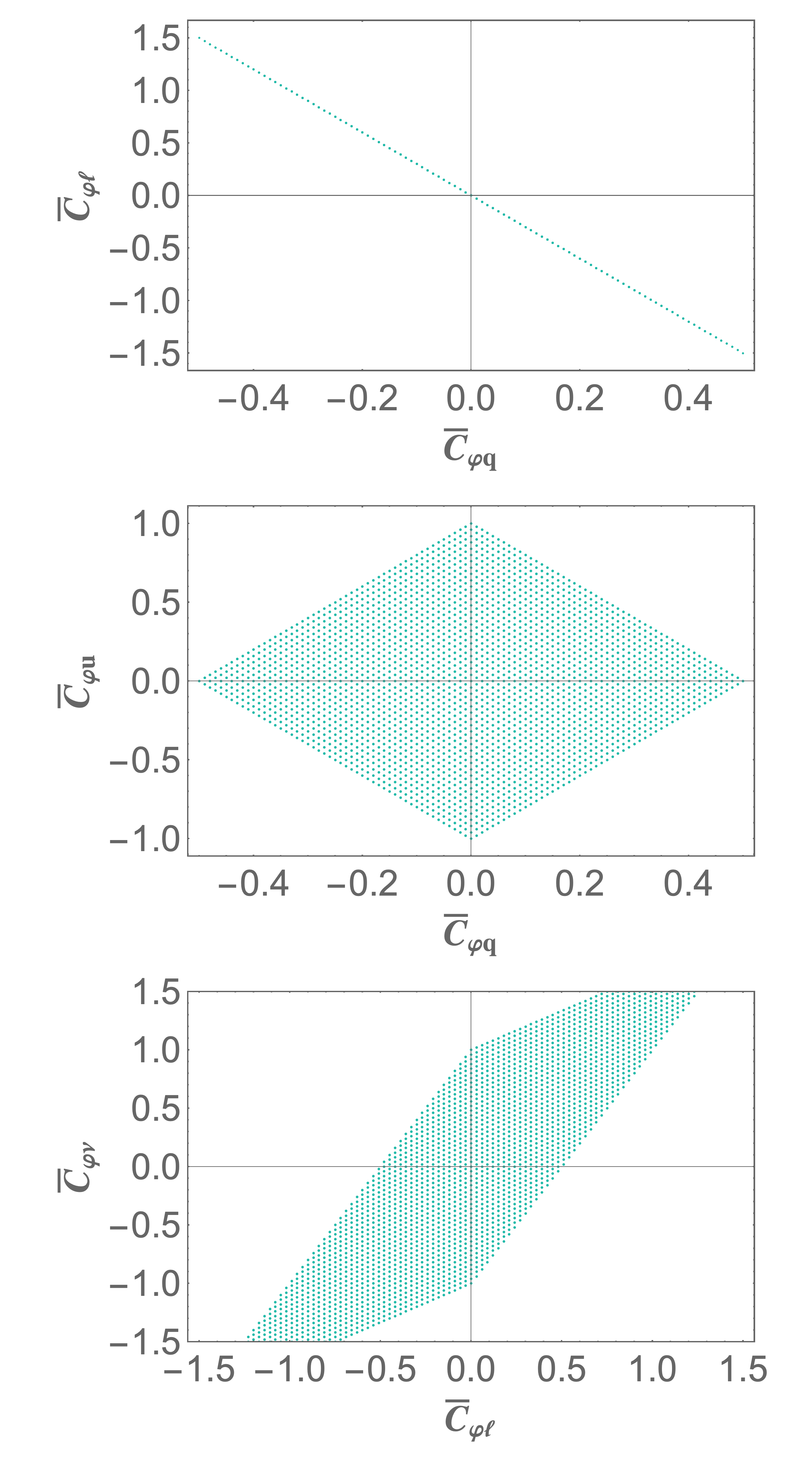
Figure 1: $Z^{\prime}$ only coupled to the third fermion generation: Correlations among nonvanishing coefficients, varying ${\bar{C}}_{\varphi d}$ and ${\bar{C}}_{\varphi e}$ in the range $[-1,1]$.

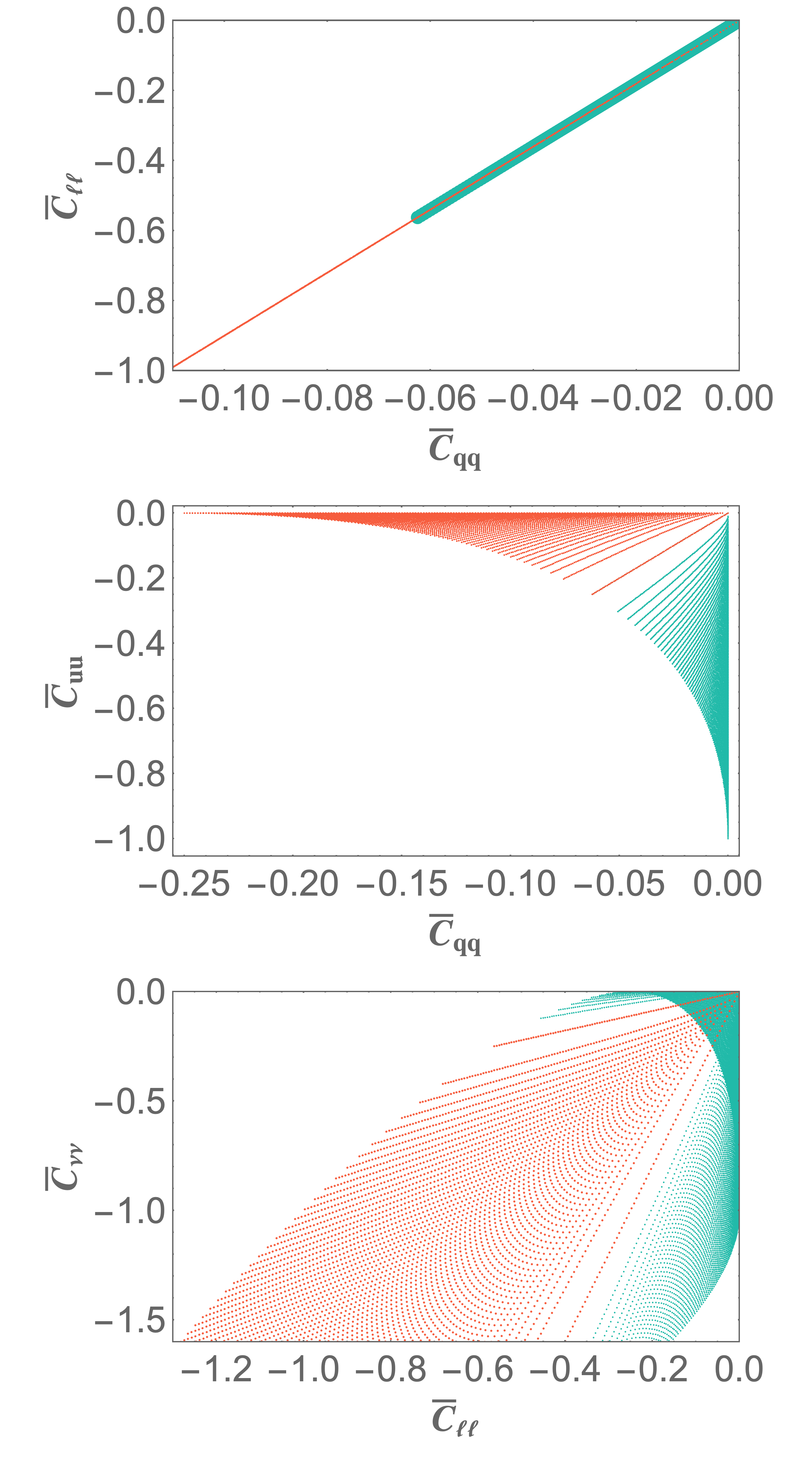
Figure 2: $Z^{\prime}$ only coupled to the third generation: Correlation among nonvanishing coefficients, varying ${\bar{C}}_{dd}$ and ${\bar{C}}_{ee}$ in the range $[-1,0]$. The green points refer to same-sign ${\bar{C}}_{dd}$ and ${\bar{C}}_{ee}$, the orange points to the case of opposite signs.

In this specific scenario, information can also be obtained on $\left[C_{\psi\psi}\right]_{\underline{3}\,\underline{3}}$. Indeed, Eqs. (15)-(19) imply

$$z_{\psi_{i}}=\pm\left(2\,\frac{M_{Z^{\prime}}^{2}}{g_{Z}^{2}}\right)^{1/2}\,\Big{(}-\big{[}C_{\psi\psi}\big{]}_{{\underline{i}}\,{\underline{i}}}\Big{)}^{1/2}\;.$$ (86)

As done for $C_{\varphi\psi}$ we define $\left[C_{\psi\psi}\right]_{\underline{3}\,\underline{3}}={\bar{C}_{\psi\psi}}.$ The ACE can be used to relate the nonvanishing $z$-hypercharges:

$$z_{q_{3}} = \frac{1}{4}\,\big{(}z_{d_{3}}-z_{e_{3}}\big{)}\,$$

$$z_{u_{3}} = -\frac{1}{2}\,\big{(}z_{d_{3}}+z_{e_{3}}\big{)}\,$$

$$z_{\ell_{3}} = -{3\over 4}\,\big{(}z_{d_{3}}-z_{e_{3}}\big{)}\,$$ (87)

$$z_{\nu_{3}} = {1\over 2}\,\big{(}z_{e_{3}}-3\,z_{d_{3}}\big{)}\;.$$

Two different cases can be analyzed, depending whether $z_{d_{3}}$ and $z_{e_{3}}$ have same or opposite signs:

• $z_{d_{3}}>0,\,\,z_{e_{3}}>0$ and $z_{d_{3}}<0,\,\,z_{e_{3}}<0$: we have

  $${\bar{C}_{qq}} = -\left({\sqrt{-{\bar{C}_{dd}}}-\sqrt{-{\bar{C}_{ee}}}\over 4}\right)^{2}\,$$

  $${\bar{C}_{uu}} = -\left({\sqrt{-{\bar{C}_{dd}}}+\sqrt{-{\bar{C}_{ee}}}\over 2}\right)^{2}\,$$

  $${\bar{C}_{\ell\ell}} = -{9\over 16}\,\left(\sqrt{-{\bar{C}_{dd}}}-\sqrt{-{\bar{C}_{ee}}}\right)^{2}\,$$ (88)

  $${\bar{C}_{\nu\nu}} = -\left({\sqrt{-{\bar{C}_{ee}}}-3\,\sqrt{-{\bar{C}_{dd}}}\over 2}\right)^{2}\;,$$

• $z_{d_{3}}<0$, $z_{e_{3}}>0$, and $z_{d_{3}}>0$, $z_{e_{3}}<0$: we have

  $${\bar{C}_{qq}} = -\left({\sqrt{-{\bar{C}_{dd}}}+\sqrt{-{\bar{C}_{ee}}}\over 4}\right)^{2}\,$$

  $${\bar{C}_{uu}} = -\left({\sqrt{-{\bar{C}_{dd}}}-\sqrt{-{\bar{C}_{ee}}}\over 2}\right)^{2}\,$$

  $${\bar{C}_{\ell\ell}} = -{9\over 16}\,\left(\sqrt{-{\bar{C}_{dd}}}+\sqrt{-{\bar{C}_{ee}}}\right)^{2}\,$$ (89)

  $${\bar{C}_{\nu\nu}} = -\left({\sqrt{-{\bar{C}_{ee}}}+3\sqrt{-{\bar{C}_{dd}}}\over 2}\right)^{2}\;.$$

Correlations among the four coefficients are obtained varying ${\bar{C}}_{dd}$ and ${\bar{C}}_{ee}$, as shown in Fig. 2.

VI.2 $Z^{\prime}$ only coupled to left-handed fermions

The possibility that $Z^{\prime}$ only couples to fermions of a given chirality has been considered, e.g., in [35]. If $Z^{\prime}$ only couples to left-handed fermions the nonvanishing coefficients are $\big{[}C_{\varphi\psi}\big{]}_{\underline{i}}$ for $\psi=\{q_{i},\,\ell_{i}\}$, hence 6 parameters. The number of constraints is reduced to 4 since Eqs. (72) and (73) are redundant. The linear equations (71) and (74) provide the relations

$${\tilde{C}}_{\varphi q}={\tilde{C}}_{\varphi\ell}=0\;.$$ (90)

The quadratic and cubic ACE provide further relations, hence the number of independent coefficients is 2. Varying $[C_{\varphi\ell}]_{\underline{3}}$ and $[C_{\varphi q}]_{\underline{3}}$, correlations are obtained among the remaining coefficients. They are shown in Fig. 3.

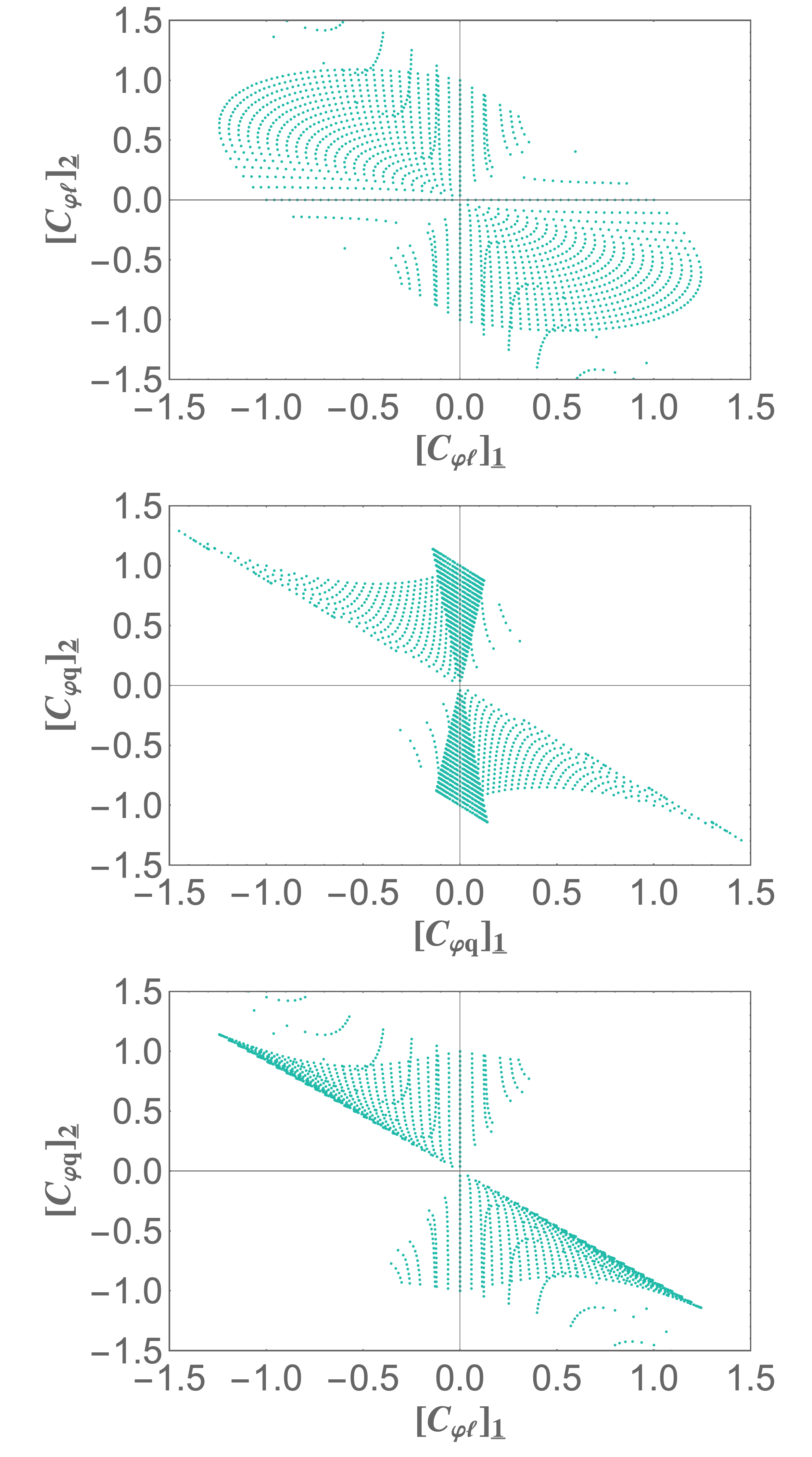
Figure 3: $Z^{\prime}$ only coupled to left-handed fermions: Correlation among nonvanishing coefficients, varying $[C_{\varphi\ell}]_{\underline{3}}$ and $[C_{\varphi q}]_{\underline{3}}$ in the range $[-1,1]$.

Also in this case the ACE can be exploited to derive correlations among $\left[C_{\psi\psi}\right]$, choosing $\left[C_{\ell\ell}\right]_{\underline{3}\,\underline{3}},\,\left[C_{qq}\right]_{\underline{3}\,\underline{3}}$ as independent coefficients, for same-sign or opposite-sign $z_{\ell_{3}}$ and $z_{q_{3}}$. The correlations between the remaining coefficients $\left[C_{\ell\ell}\right]_{\underline{3}\,\underline{3}}$ and $\left[C_{qq}\right]_{\underline{3}\,\underline{3}}$ are shown in Fig. 4.

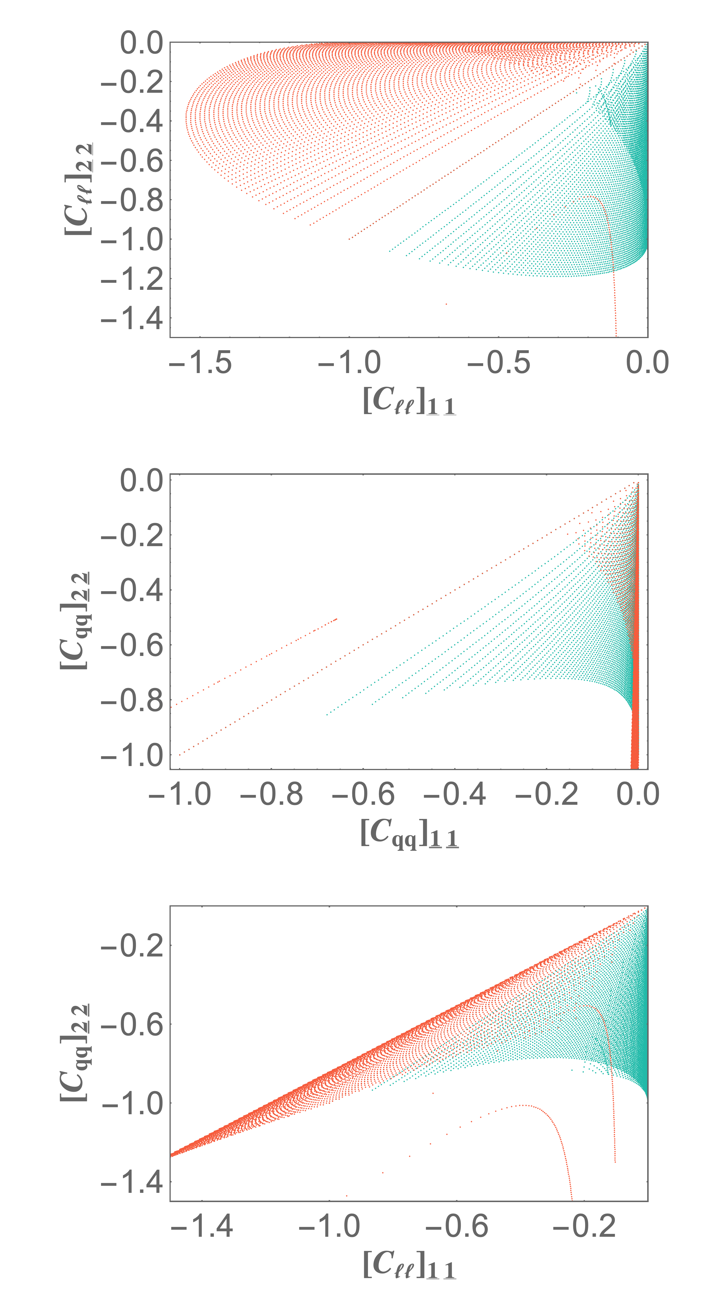
Figure 4: $Z^{\prime}$ coupled only to left-handed fermions: Correlations among coefficients, varying $\left[C_{\ell\ell}\right]_{\underline{3}\,\underline{3}}$ and $\left[C_{qq}\right]_{\underline{3}\,\underline{3}}$ in the range $[-1,0]$. The color code is the same as in Fig. 2.

VI.3 $Z^{\prime}$ only coupled to right-handed fermions

If $Z^{\prime}$ only couples to right-handed fermions, the nonvanishing coefficients are $\big{[}C_{\varphi\psi}\big{]}_{\underline{i}}$ for $\psi=\{u_{i},\,d_{i},e_{i},\nu_{i}\}$, hence 12 parameters. The number of constraints is reduced to 5 since Eq. (72) is automatically satisfied. Eqs. (71), (73) and (74) provide the relations

$${\tilde{C}}_{\varphi u}=-{\tilde{C}}_{\varphi d}=-{\tilde{C}}_{\varphi e}={\tilde{C}}_{\varphi\nu}\;.$$ (91)

The quadratic and cubic ACE give further relations, so that the number of independent coefficients is 7.

VI.4 Leptophobic $Z^{\prime}$

If $Z^{\prime}$ only couples to quarks, the nonvanishing coefficients are $\big{[}C_{\varphi\psi}\big{]}_{\underline{i}}$ for $\psi=\{q_{i},\,u_{i},\,d_{i}\}$, therefore 9 parameters. The number of constraints is 5, since Eq. (74) is automatically verified. The other linear equations provide the relations

$${\tilde{C}}_{\varphi q}={\tilde{C}}_{\varphi u}={\tilde{C}}_{\varphi d}=0\;,$$ (92)

while the quadratic and cubic ACE read

$${\tilde{C}}_{\varphi q}^{(2)}-2\,{\tilde{C}}_{\varphi u}^{(2)}+{\tilde{C}}_{\varphi d}^{(2)}=0\;$$ (93)

$$2\,{\tilde{C}}_{\varphi q}^{(3)}-{\tilde{C}}_{\varphi u}^{(3)}-{\tilde{C}}_{\varphi d}^{(3)}=0\;.$$ (94)

Consequently, there are 4 independent coefficients.

VI.5 Hadrophobic $Z^{\prime}$

The situation is specular to the leptophobic $Z^{\prime}$. The expressions of the ACE are

$${\tilde{C}}_{\varphi\ell}={\tilde{C}}_{\varphi\nu}={\tilde{C}}_{\varphi e}=0\;$$

$$-{\tilde{C}}_{\varphi\ell}^{(2)}+{\tilde{C}}_{\varphi e}^{(2)}=0\;$$ (95)

$$2\,{\tilde{C}}_{\varphi\ell}^{(3)}-{\tilde{C}}_{\varphi\nu}^{(3)}-{\tilde{C}}_{\varphi e}^{(3)}=0\;.$$

The number of independent coefficients is 4.

For such models the experimental bounds are weaker than in previous cases, and allow a relatively light $Z^{\prime}$. Moreover, $Z^{\prime}$ can contribute to lepton-flavour violating decays and to the lepton anomalous magnetic moments [36, 37, 38, 39, 40, 41, 42, 43], an issue of great interest at present [44, 45]. Models gauging $L_{a}-L_{b}$ ($a,b$ being the lepton flavours) belong to this class, namely models gauging $L_{\mu}-L_{\tau}$ [46, 47, 48, 49, 50, 51].

As an example of a hadrophobic model, we can also consider the $Z^{\prime}$ only coupled to right-handed neutrinos, a scenario belonging to the class of neutrinophilic NP models [52, 53, 54]. As for the ACE, setting all z-hypercharges to $0$ but for right-handed neutrinos, we have that Eq. (95) is satisfied only if at least one of the three right-handed neutrinos is sterile under $\text{U}(1)^{\prime}$. Choosing $z_{\nu_{3}}=0$, the ACE imply $\left[C_{\varphi\nu}\right]_{\underline{3}}=0$ and $\left[C_{\varphi\nu}\right]_{\underline{1}}=-\left[C_{\varphi\nu}\right]_{\underline{2}}$.

VI.6 ABCD model [23]

A model with a heavy gauge boson $Z^{\prime}$ with flavour nonuniversal quark and lepton couplings has been considered in [23]. The assignment of the $z$-hypercharge to a generic fermion $\psi_{i}=\{q_{i},\,u_{i},\,d_{i},\,\ell_{i},\,\nu_{i},\,e_{i}\}$ ($i$ a generation index) is

$$z_{\psi_{i}}=y_{\psi}+\epsilon_{i}\;.$$ (96)

$y_{\psi}$ denote the generation universal SM hypercharges, $\epsilon_{i}$ are parameters generation dependent, but universal within a given generation. This construction produces quark-lepton correlations. As shown in [23], all ACE are satisfied provided

$$\sum_{i=1}^{3}\epsilon_{i}=0\;.$$ (97)

The assignment implies the relation

$${\tilde{C}}_{\varphi\psi} = 3\,\left(-{g_{Z}^{2}\,C_{\varphi D}\over 2\,M_{Z^{\prime}}^{2}}\right)^{1/2}\,y_{\psi}\;.$$ (98)

For right-handed neutrinos one has ${\tilde{C}}_{\varphi\nu}=0$ since $y_{\nu}=0$. Nontrivial relations among the SMEFT coefficients are predicted:

$$-6\,\frac{{\tilde{C}}_{\varphi q}}{{\tilde{C}}_{\varphi e}}=-\frac{3}{2}\,\frac{{\tilde{C}}_{\varphi u}}{{\tilde{C}}_{\varphi e}}=3\,\frac{{\tilde{C}}_{\varphi d}}{{\tilde{C}}_{\varphi e}}=2\,\frac{{\tilde{C}}_{\varphi\ell}}{{\tilde{C}}_{\varphi e}}\;.$$ (99)

VII Conclusions

The possibility of gaining information on possible extensions of the SM, in a bottom-up approach, is largely based on the SM effective field theory framework. It is important to obtain the widest information from the phenomenological analysis of the coefficients of the operators in the effective field theory Lagrangian. We have discussed the set of constraints and relations among the coefficients of the $d=6$ operators if the SM extension includes a non-anomalous $\text{U}(1)^{\prime}$. In particular, we have investigated how the anomaly cancellation equations, involving the $z$-hypercharges, can be translated into constraints for the $\nu$SMEFT Wilson coefficients. Such constraints become more stringent if particular features are assumed for the $Z^{\prime}$ couplings to fermions. We have discussed examples on how the constraints can be exploited, and which correlations among the coefficients emerge. The search for such correlations in experimental measurements is a way for accessing the long-sighted extension of the Standard Model.