GridPE: Unifying Positional Encoding in Transformers with a Grid Cell-Inspired Framework

Abstract

Understanding spatial location and relationships is a fundamental capability for modern artificial intelligence systems. Insights from human spatial cognition provide valuable guidance in this domain. Recent neuroscientific discoveries have highlighted the role of grid cells as a fundamental neural component for spatial representation, including distance computation, path integration, and scale discernment. In this paper, we introduce a novel positional encoding scheme inspired by Fourier analysis and the latest findings in computational neuroscience regarding grid cells. Assuming that grid cells encode spatial position through a summation of Fourier basis functions, we demonstrate the translational invariance of the grid representation during inner product calculations. Additionally, we derive an optimal grid scale ratio for multi-dimensional Euclidean spaces based on principles of biological efficiency. Utilizing these computational principles, we have developed a Grid-cell inspired Positional Encoding technique, termed GridPE, for encoding locations within high-dimensional spaces. We integrated GridPE into the Pyramid Vision Transformer architecture. Our theoretical analysis shows that GridPE provides a unifying framework for positional encoding in arbitrary high-dimensional spaces. Experimental results demonstrate that GridPE significantly enhances the performance of transformers, underscoring the importance of incorporating neuroscientific insights into the design of artificial intelligence systems.

1 Introduction

Understanding how the mammalian brain represents spatial characteristics and relationships remains a critical question in cognitive science and neuroscience. Specifically, the focus is on identifying the neural bases and their roles in self-localization, navigation, and path planning. Scholars have conducted extensive research to address this question. [1] designed an animal experiment where rats performed a wayfinding task in a radial maze, introducing the concept of the cognitive map to describe the internal environmental representation that supports flexible spatial behavior. Subsequent discoveries identified the neural cellular basis of the cognitive map in the mammalian brain, a line of research that earned the Nobel Prize in 2014. Place cells activate when a mammal enters an area near a specific spatial location [2, 3], and are believed to distinguish and represent different places. Grid cells in the medial entorhinal cortex (MEC), on the other hand, exhibit periodic, hexagonal, and grid-like firing fields [4]. These cells are thought to define distance metrics in Euclidean space, support multi-scale self-localization, and facilitate path integration and vector-based navigation [5, 6, 7]. In other words, grid cells represent spatial relationships independently of the agent’s current visual sensory input and head direction (referred to as "allocentric" representation). Due to their close association with spatial representation, the principles of grid cell firing have been widely adopted by artificial intelligence researchers beyond neuroscience, including in robotics navigation system design [8], reinforcement learning agent trajectory planning [9], and positional encoding for geospatial data [10, 11].

There are at least two approaches to incorporating grid cells into AI systems. For bottom-up approach, agents can learn from trajectory experience (i.e., model training in the context of machine learning), and grid-like firing patterns can often emerge from certain neuron activations in the architecture [7, 12]. While these agent architectures validate the existence of grid cells, they struggle to directly encode spatial positions from knowledge of the model. For the top-down methods, researchers intentionally design computational models to simulate grid cell firing and integrate them into the agent for navigation. Two commonly adopted techniques are the continuous attractor network (CAN) and the velocity-controlled oscillator (VCO). The CAN model constructs a recurrent neural network that takes velocity input to compute a steady state from this neural dynamic system, simulating grid cells [13]. However, CAN presumes symmetric connections and regular cellular arrangement in the network, which rarely hold true in authentic neural anatomical structure [14]. VCO models assume that grid cell firing patterns arise from the interference of oscillations with distinct frequencies [15]. A grid cell’s activation pattern can be the summation of three planar waves with respective frequency direction vectors, each separated by 120°[16]. VCO models encode location with high simplicity and are theoretically supported by neuroscience evidence such as band cells [17] and phase precession phenomena in bats [18, 19].

Building on the advantages of the VCO model for explaining grid cells, this paper mathematically models grid cells based on VCO model assumptions. The activation intensity of a grid cell within a high-dimensional Euclidean space can be derived as the summation of Fourier basis functions. For example, a one-dimensional Euclidean space can be represented by one Fourier basis, while a two-dimensional Euclidean space can be represented by three Fourier bases. We first prove that the inner product of two grid cells can map to the metric endowed on Euclidean space, and we further demonstrate that grid cells can be represented as multi-dimensional vectors through Random Fourier Feature (RFF) computation. Following the economic principle of achieving the highest spatial resolution with the fewest cells, we derived the theoretically optimal scale ratio.

Inspired by the spatial encoding properties of grid cells, we designed a positional encoding scheme named GridPE for representing multi-dimensional spatial positions in self-attention architectures. To compare GridPE with classical positional encoding techniques, we conducted experiments using the Pyramid Vision Transformer (PVT) architecture [20] on the ImageNet-1000 image classification task [21]. The results demonstrate its effectiveness in enhancing the self-attention mechanism by providing both absolute and relative positional information, highlighting the potential of integrating neuroscience findings into AI system design.

2 Preliminaries

We model the grid cell on the theoretical basis of VCO theory [15, 22]. Under this assumption, presynaptic cells of the grid cell (sometimes referred to as "simple cells" [14]) perform oscillations similar to two-dimensional planar waves, forming parallel band "strips" along specific directions. The oscillation frequency of the presynaptic dendrites is sensitive to the agent’s current velocity, which is why the theory is named "velocity-controlled." The frequency can be expressed as the result of modulating the somatic oscillation base frequency, with the modulation magnitude depending on the velocity vector and the presynaptic preferred direction (or wave vector of the planar wave) [9].

$$\frac{d}{dt}\varphi=\omega_{d}=\omega_{s}+\beta\boldsymbol{v}^{T}\boldsymbol{k}$$ (1)

where $\omega_{s}$ is the somatic base frequency, usually experimentally measured as theta wave frequency (4-11 Hz) [9]. $\boldsymbol{v},\boldsymbol{k}\in\mathbb{R}^{2}$ are the velocity vector and wave vector in the two-dimensional space, the latter indicating preferred direction and wave length. $\beta$ is a position factor deciding sensitivity to velocity. The velocity-modulated dendrite frequency $\omega_{d}$ is the derivative of oscillation phase $\phi$. Here, we do not differentiate between angular velocity and frequency due to their constant ratio of $2\pi$. When we integrate the modulated frequency over the time $t$, we obtain the oscillation phase:

$$\varphi(t)-\varphi(0)=\int_{0}^{t}(\omega_{s}+\beta\boldsymbol{v}^{T}\boldsymbol{k})\,dt=\omega_{s}t+\beta\boldsymbol{k}^{T}\boldsymbol{x}$$ (2)

where $\boldsymbol{x}$ is the displacement vector from time $0$ to time $t$. Clearly, at a given time, locations with the same projection onto the wave vector correspond to the same oscillation phase, thus form a parallel activation bands across the environments when we calculate amplitude. If we overlap multiple such presynaptic firing fields with weights, we can obtain grid cell hexagonal firing patterns. The oscillation is expressed as Fourier basis function, and grid cell activation at any location can be expressed as [23]:

$$g =\sum_{i=0}^{n}c_{i}\,e^{j\omega_{s}t}\cdot e^{j\beta\boldsymbol{k}_{i}^{T}\boldsymbol{x}}$$ (3)

$$=\sum_{i=0}^{n}c_{i}(t)e^{j\boldsymbol{k}_{i}^{T}\boldsymbol{x}}$$

Imagery unit is denoted as $j$, and the number of presynampic cells is denoted as $n$. We omit the $\beta$ which can be integrated into wave vector $k$. For the second equality, the time-dependent function $c_{i}(t)$ combine the information of synaptic weight and somatic base oscillation, while the factor of Fourier basis only depend on location $x$. That means the temporal fluctuation of the activation is only driven by the intrinsic theta waves evolving as time progresses, which is independent from spatial representation. Therefore, we can fix to a certain time point and discuss the grid cell representation across the space from a static viewpoint, for which we omit the time variable $t$ in the following derivation. In previous research, three Fourier bases with their directional preferences forming angles of 120° between each other are commonly used [23, 16], as illustrated in Figure 1.

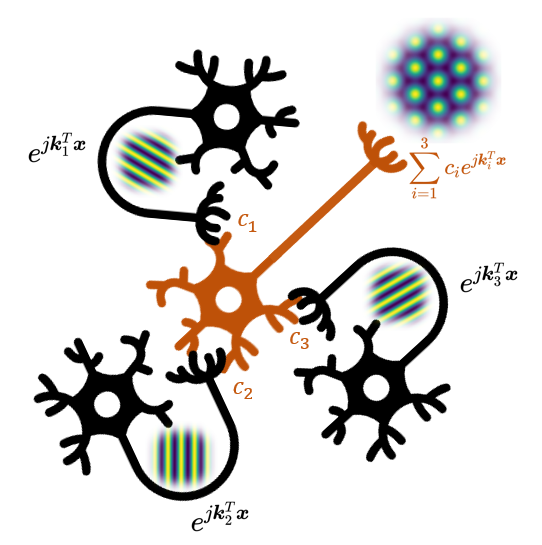
Figure 1: Illustration of VCO theory. The black neurons are presynaptic neurons with simple oscillation in their dendrites. The orange neuron is the grid cell, whose grid firing pattern results from the summation of the three oscillation with different preferred direction.

3 Derivation of Grid Cell Positional Encoding

3.1 Inner Product Translational Invariance

Grid cells are not only responsible for representing absolute locations in Euclidean space but are also expected to encode relative spatial shifts between locations. This allows for the representation of free vectors from any starting location within the space, thereby facilitating vector-based navigation. The inner product of grid cell representations provides valuable insights into this capability. For a single grid cell, its representation at location $\boldsymbol{x}$ is given by:

$$g(\boldsymbol{x})=\sum_{i=0}^{n}c_{i}e^{j\boldsymbol{k}_{i}^{T}\boldsymbol{x}}$$ (4)

Assume that $\boldsymbol{x}$ deviates from $\boldsymbol{y}$ by a fixed vector $\boldsymbol{d}$ (i.e., $\boldsymbol{x}-\boldsymbol{y}=\boldsymbol{d}$). We then compute the functional inner product of $g(\boldsymbol{x})$ with itself over the Euclidean space, that is.

$$\left\langle g(\boldsymbol{x}),g(\boldsymbol{y})\right\rangle_{\mathcal{H}} =\int_{\mathcal{X}}\sum_{i=0}^{n}\sum_{m=0}^{n}c_{i}c_{m}^{*}e^{j(\boldsymbol{k}_{i}-\boldsymbol{k}_{m})^{T}\boldsymbol{x}}e^{j\boldsymbol{k}_{m}^{T}(\boldsymbol{x}-\boldsymbol{y})}$$ (5)

$$=\sum_{i=0}^{n}|c_{i}|^{2}e^{j\boldsymbol{k}_{i}^{T}\boldsymbol{d}}$$

That means for a given grid cell, the inner product of its activation map and its shifted version can represent the shift vector without consideration of any certain locations. Apparently, the inner product form a tranlational invariant kernel function $\kappa_{0}(\boldsymbol{x},\boldsymbol{y})=\left\langle g(\boldsymbol{x}),g(\boldsymbol{y})\right\rangle_{\mathcal{H}}=h(\boldsymbol{x}-\boldsymbol{y})$. There are countless grid cells in the mammal’s brain. The collective representation to the offset vector $\boldsymbol{d}$ can be expressed as follow as the summation of grid cell inner products:

$$\sum_{g\in\mathcal{G}}\left\langle g(\boldsymbol{x}),g(\boldsymbol{y})\right\rangle_{\mathcal{H}}=\sum_{i}|c_{i}|^{2}e^{j\boldsymbol{k}_{i}^{T}\boldsymbol{d}}\propto\int_{\mathbb{R}^{2}}p(\boldsymbol{k})|c(\boldsymbol{k})|^{2}e^{j\boldsymbol{k}^{T}\boldsymbol{d}}\,d\boldsymbol{k}$$ (6)

Note this function is also a translational invariant kernel for $\boldsymbol{x}$ and $\boldsymbol{y}$. Simultaneuously, in its form it scale to the inverse Fourier transformation of the probability distribution of wave vectors. According to Bochner theorem [24], we know this kernel, as the inverse Fourier transformation of a non-nagative measurement, is positive definite. Therefore, we can apply random Fourier feature (RFF) [25] technique on this shift-invariant kernel, which demands positive definite kernel as the prerequisite. We denote the $\kappa(\boldsymbol{x},\boldsymbol{y})$ as this kernel and we can know:

$$\kappa(\boldsymbol{x},\boldsymbol{y}) =\int_{\mathbb{R}^{2}}p(\boldsymbol{k})|c(\boldsymbol{k})|^{2}e^{j\boldsymbol{k}^{T}\boldsymbol{d}}\,d\boldsymbol{k}$$ (7)

$$=\mathbb{E}_{\boldsymbol{k}}\left[|c(\boldsymbol{k})|^{2}e^{j\boldsymbol{k}^{T}\boldsymbol{d}}\right]$$

$$\approx\frac{1}{D}\sum_{i=1}^{D}\left(|c_{i}|^{2}e^{j\boldsymbol{k}_{i}^{T}\boldsymbol{x}}\cdot e^{-j\boldsymbol{k}_{i}^{T}\boldsymbol{y}}\right)$$

$$=\frac{1}{\sqrt{D}}\left(\begin{array}[]{c}e^{j\boldsymbol{k}_{1}^{T}\boldsymbol{x}}\\ e^{j\boldsymbol{k}_{2}^{T}\boldsymbol{x}}\\ \vdots\\ e^{j\boldsymbol{k}_{D}^{T}\boldsymbol{x}}\end{array}\right)^{T}\begin{bmatrix}|c_{1}|^{2}&&&\\ &|c_{2}|^{2}&&\\ &&\ddots&\\ &&&|c_{D}|^{2}\end{bmatrix}\left(\begin{array}[]{c}e^{-j\boldsymbol{k}_{1}^{T}\boldsymbol{y}}\\ e^{-j\boldsymbol{k}_{2}^{T}\boldsymbol{y}}\\ \vdots\\ e^{-j\boldsymbol{k}_{D}^{T}\boldsymbol{y}}\end{array}\right)\frac{1}{\sqrt{D}}$$

When considering the population activity of grid cells, we can disregard the constant $\frac{1}{\sqrt{D}}$ that represents the population size. In this context, grid cells can be seen as the product of diagonalized input weights and a vector whose entries are Fourier bases with preferred directional preferences. This is analogous to Fourier analysis, where a function is decomposed into orthogonal bases and their corresponding coefficients. Consequently, the inner product of spatial-domain representation functions in the functional space is replaced by the inner product of frequency-domain vectors in a finite-dimensional vector space.

We propose that the brain represents Euclidean space using multi-dimensional Fourier analysis, akin to the auditory system’s information processing. By integrating oscillations of various spatial frequencies, the grid cell encoding system can efficiently represent spatial information with high resolution. Furthermore, the Random Fourier Features (RFF) approach imposes no constraints on the dimensionality of locations $\boldsymbol{x}$ and $\boldsymbol{y}$. This suggests that the Fourier representation of grid cells can encode location information in arbitrarily high-dimensional spaces.

3.2 Optimal Ratio of Grid Scale under Economy Principle

In the derivation above, we assumed the wave vector (i.e., the preferred direction) follows a probability distribution, such as the uniform distribution often used in RFF. However, neuroscience evidence shows that the medial entorhinal cortex consists of several modules. Within the same module, the direction and period scale of the cell grids remain consistent, but these discretized scales shrink along the ventral-dorsal axis [26], representing a transition from coarse, low-frequency to granular, high-frequency spatial information. The periodic ratio of the adjacent scale remains around 1.5, as estimated by both animal measurements and computational simulations [26, 7]. This hierarchical spatial representation demands significantly fewer grid cells while maintaining fine spatial resolution, or say the economy principle [27].

The challenge now is to determine the optimal ratio of the grid scale, which is crucial for constructing a positional encoding system. Recall that in the original positional encoding of the Transformer architecture [28], the encoding spatial frequency is calculated as $\omega_{k}=\frac{1}{10000^{2k/d}}$, forming a geometric series of wavelengths. The rationale behind this choice remains unclear, and we anticipate that computational theories of grid cells can provide insights into frequency determination.

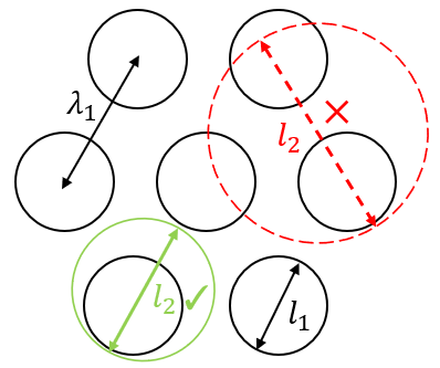
Figure 2: Illastration of relationship between firing fields diameter and periodicity. For two grid cells with adjacent discrete scale, the periodcity of the smaller scale must be less than the diameter of the larger one, otherwise the system cannot distinguish two locations.

Here we provide a generalized derivation based on the proof in [27]. We aim to represent p-dimensional Euclidean space with the least number of grid cells, reflecting the principle of economy. Assume there are $m$ scales (or layers) of the grid cells. The period of the $i$-th module layer ($i=1,2,\ldots,m$), or the distance between the adjacent grid vertices, is denoted as $\lambda_{i}$. The period increase as $i$ becomes larger. The scale ratio of the adjacent layers is $r=\lambda_{i+1}/\lambda_{i}>1$. A grid field is a hyperspherical area centered around a grid vertex in the space, with its diameter denoted as $l_{i}$. For 2D space, a grid field is a circular-plate area activating the grid cell. Clearly, to cover the whole space without omissions, more than one grid cell with different phases are required. The larger the ratio of $\lambda_{i}$ to $l_{i}$, the more grid cells are needed. If there must be at least $d$ cells responding to a spatial location, the total number of grid cells across all layers can be expressed as $N$:

$$N=\sum_{i=1}^{m}d\left(\frac{\lambda_{i}}{l_{i}}\right)^{p}$$ (8)

Apart from that, the condition $l_{i}\leq\lambda_{i-1}$ must be satisfied. If not, the grid cell system cannot ascertain current location when cells from both layer $i$ and $i+1$ fire simultaneously, because the larger firing field contains more than one smaller fields, as shown in Figure 2. The condition derives $l_{i}\leq\lambda_{i}/r$. If the grid cell system must represent the space at a given constant spatial resolution $R$, that is, we predefined the measurement relationship between the largest scale and the smallest firing field unit:

$$R=\left(\frac{\lambda_{m}}{l_{1}}\right)^{p}=\left(\prod_{i=0}^{m-1}\frac{\lambda_{i+1}}{\lambda_{i}}\right)^{p}=\left(r^{p}\right)^{m}$$ (9)

Here we set the $\lambda_{0}=l_{1}$. When we denote $r^{p}=\rho$ we get:

$$N=d\sum_{i=1}^{m}\left(\frac{\lambda_{i}}{l_{i}}\right)^{p}\geq dmr^{p}=d\rho\log_{\rho}R$$ (10)

By differentiation, we find that when $\rho=e$, which means $r=\sqrt[p]{e}$, we achieve the minimal number of grid cells, adhering to the principle of economy. In summary, a hierarchical grid cell representation can, with a limited population number, efficiently cover the space. The theoretically optimal scale ratio for $p$-dimensional space is $r=\sqrt[p]{e}$.

3.3 Proposal of Grid-cell Positional Encoding (GridPE)

After demonstrating the capability of representing relative movement in space through inner product calculations and determining the optimal ratio of encoding periods, we introduce a novel positional encoding scheme for attention-based architectures. Inspired by neuroscientific principles of grid cells, our method extends the foundational ideas presented by  [29]. While Su’s model combines absolute and relative positional encodings within a fixed framework, our schema advances this by incorporating grid cell-inspired encodings that inherently support extrapolation to higher dimensions and maintain translational invariance. Notably, in one-dimensional space, where GridPE can be expressed using a single Fourier basis, our encoding scheme is equivalent to rotational positional encoding. This demonstrates the flexibility of our approach and its alignment with established encoding strategies, further enhancing its applicability across various architectural contexts. According to Su’s model, to accommodate both absolute and relative positional encoding, the inner product of the query $\boldsymbol{q}$ and key $\boldsymbol{k}$, which represents their similarity, can be modified as follows:

$$\left\langle\boldsymbol{q}^{\prime},\boldsymbol{k}^{\prime}\right\rangle=\boldsymbol{q}^{T}\boldsymbol{W}_{m}^{T}\boldsymbol{W}_{n}\boldsymbol{k}$$ (11)

Here $m$ and $n$ refer to the position of the query and key respectively. The multiplication of $\boldsymbol{W_{m}}$ and $\boldsymbol{W_{n}}$ is the function of the relative position $m-n$. We can encode the position $m$ based on the grid cell encoding rationale. Assume there are $d$ dimensions for the embedded queries and keys, we also set $d$ layers of different scale of grid cell. Then we can set the positional code as below:

$$\boldsymbol{W}_{m}=\left[\sum_{i}c_{i}e^{j\boldsymbol{\omega}_{i,1}^{T}m},\sum_{i}c_{i}e^{j\boldsymbol{\omega}_{i,2}^{T}m},\dots,\sum_{i}c_{i}e^{j\boldsymbol{\omega}_{i,d}^{T}m}\right]^{T}$$ (12)

Here we substitute the symbol of the wave vector $\boldsymbol{k}$ with $\boldsymbol{\omega}$ in case of confusion of key. We can see the inner product of the two positional codes $\boldsymbol{W}_{m}^{T}\boldsymbol{W}_{n}$ preserve the translational invariance. To fulfill the positional encoding in the neural network, we proposed several strategies as the variants to integrate the position information into the queries or keys.

Representing Encodings as Rotation Matrices

If the information to be encoded (query or key) is a $d$-dimensional vector, and $d$ is even, then the positional codes can be calculated as follows:

$$\boldsymbol{R}_{m}=\begin{bmatrix}\Re\left(e^{j\boldsymbol{\omega}_{1,1}^{T}m}\right)&-\Im\left(e^{j\boldsymbol{\omega}_{1,1}^{T}m}\right)&0&\dots&0&0\\ \Im\left(e^{j\boldsymbol{\omega}_{1,1}^{T}m}\right)&\Re\left(e^{j\boldsymbol{\omega}_{1,1}^{T}m}\right)&0&\dots&0&0\\ \vdots&\vdots&\ddots&\vdots\\ 0&0&0&\dots&\Re\left(e^{j\boldsymbol{\omega}_{d/2,1}^{T}m}\right)&-\Im\left(e^{j\boldsymbol{\omega}_{d/2,1}^{T}m}\right)\\ 0&0&0&\dots&\Im\left(e^{j\boldsymbol{\omega}_{d/2,1}^{T}m}\right)&\Re\left(e^{j\boldsymbol{\omega}_{d/2,1}^{T}m}\right)\\ \end{bmatrix}$$ (13)

$$\left\langle\boldsymbol{q}^{\prime},\boldsymbol{k}^{\prime}\right\rangle=\boldsymbol{q}^{T}\boldsymbol{R}_{m}^{T}\boldsymbol{R}_{n}\boldsymbol{k}$$ (14)

The $\Re(\cdot)$ and $\Im(\cdot)$ respectively means the extraction of the real and imagery part. The purpose of this strategy is to encode the position by constructing the rotation matrix. The rotation angles comes from the grid cell Fourier functions.

Incorporating Real and Imaginary Parts into Information Vectors

We can also extract the real and imagery part and add them into the information vectors, similar to the original Transformer architecture:

$$\boldsymbol{q}^{\prime}=\Re\left(\boldsymbol{W}_{m}\right)+\Im\left(\boldsymbol{W}_{m}\right)+\boldsymbol{q}$$ (15)

After the encoding, the similarity of encoded queries and key can be calculated as vector dot product.

Preserving the Complex Form

We can directly use the real part of the inner product between two sets of "complex" position encoding as the encoding product.

$$\left\langle\boldsymbol{q}^{\prime},\boldsymbol{k}^{\prime}\right\rangle=\boldsymbol{q}^{T}\Re\left(\boldsymbol{W}_{m}^{H}\boldsymbol{W}_{n}\right)\boldsymbol{k}$$ (16)

The Hermite operator means the conjugate transpose of the complex matrix.

Feature Mapping of Positional Encoding Using Deep Learning

Finally, we can transform the original positional encoding by applying a trained deep neural network.

$$\left\langle\boldsymbol{q}^{\prime},\boldsymbol{k}^{\prime}\right\rangle=\boldsymbol{q}^{T}f_{\theta}(\boldsymbol{W}_{m}^{T})f_{\theta}(\boldsymbol{W}_{n})\boldsymbol{k}$$ (17)

where $f_{\theta}(\cdot)$ is a neural network projection (e.g. a multi-layer perceptrons) parameterized by $\theta$. The projection does not change the dimension of the encoding.

4 Experiments

4.1 Property of Distance Decay

We firstly display that our positional encoding approach exhibits the property of distance decay in any high-dimensional space. This implies that the association between two positions diminishes as the distance between them increases. We select a square area in two-dimensional space, calculating the positional encoding vector within the area as Equation (12), and compute the inner products between the central "core" point and uniformly sampled points. Given that we have proven the translational invariance of the inner product, our findings remain valid when any other point is chosen as the core. Figure 3 presents the inner product surface plot and a profile plot with $x$ fixed at $0.5$.

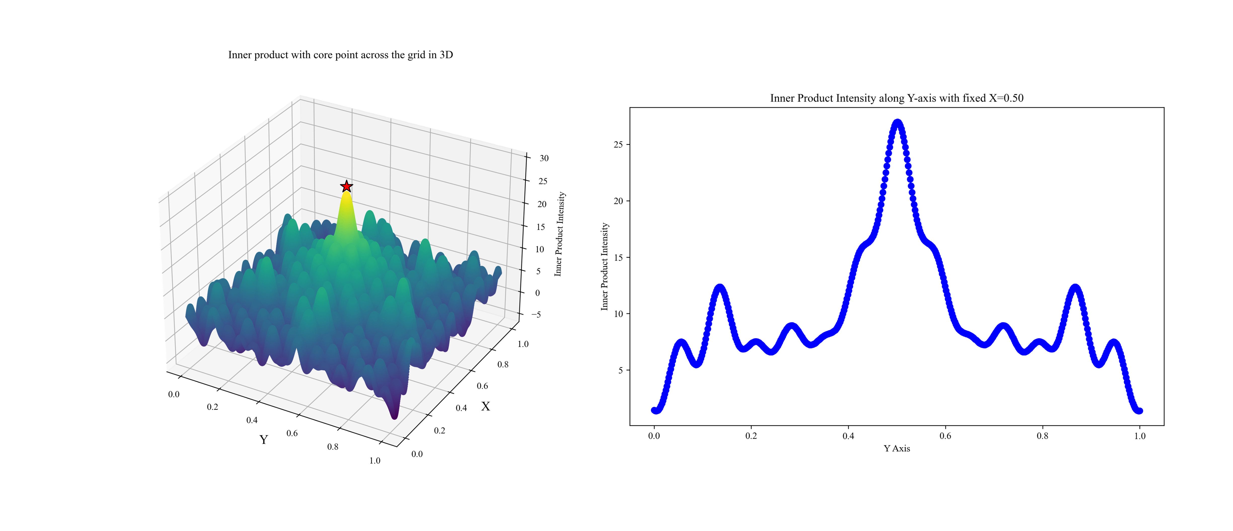
Figure 3: The inner products intensity with the core points $(0.5,0.5)$ of points in the unit square area. Left: the distribution of inner products is shown as a surface plot across the area. Right: a profile plot showing the inner products between core points and points with fixed $x=0.5$.

We observe that the inner product exhibits an overall decreasing trend as the spatial distance increases, with points near the core having relatively larger inner products. Despite this, local sinusoidal fluctuations, resulting from the Fourier function form, are still evident. These calculations corroborate the effectiveness of our encoding method in representing spatial distance relationships.

4.2 Performance of GridPE on Visual Task

To empirically validate the capability of GridPE strategies to encode positional information, we draw on previous research [30, 31] and design a image classification task to evaluate neural network architectures with different positional encodings. We select the Pyramid Vision Transformer (PVT) as the base architecture [20]. PVT, a classic variant of the Vision Transformer, introduces a pyramid structure that reduces input resolution and computation cost, thereby enhancing task performance.

We utilize the ImageNet-100 dataset to design the classification task. We evenly select ten classes, and for each class, we pick 250 images. Among them, 50 evenly chosen images are partitioned as the validation set, while the other 200 are used for training. We compare seven models with different positional encoding choices. All positional encoding approaches are applied to the base attention-based structure. PVT-o refers to the original PVT architecture with no explicit two-dimensional positional encoding. PVT-abs refers to applying classical and sinusoidal two-dimensional positional encoding to image pixels [28]. CPVT is a variant of PVT with conditional positional encoding [31]. GridPVT-rotate, GridPVT-merge, GridPVT-complex, and GridPVT-deep correspond to the models enhanced with the four aforementioned GridPE encoding methods, respectively. We train the neural networks on a device with a Ubuntu 22.04 operation system, an Intel Xeon Platinum 8352V CPU, and an NVIDIA RTX 4090 GPU. The model are trained on the training set for 200 epochs, with AdamW optimizer.

The performance of all trained models on the validation set is shown in Table 1. We can see that our proposed GridPVT model supported by GridPE enhances classification performance to some extent. Although GridPVTs display similar performance to CPVT in the top-1 prediction task, for top-5 classification, the accuracy of GridPVT models generally surpasses that of the other three models. Among the four GridPVTs, the model with positional code merging and neural network projection achieves better accuracy scores than the others.

Table 1: Comparative Analysis of Different Position Encoding Methods in Image Classification Tasks

Model Name	Acc@1 (%)	Acc@5 (%)	Loss
PVT-o	58.6	92.8	1.467
CPVT	60.6	91.8	1.498
PVT-abs	58.6	92.8	1.483
GridPVT-rotate	54.2	93.4	1.511
GridPVT-merge	56.0	94.8	1.507
GridPVT-complex	56.4	93.6	1.514
GridPVT-deep	59.2	94.2	1.445

5 Conclusion

Positional encoding is crucial for artificial intelligence as it elucidates how information is effectively organized within neural networks. This study introduces GridPE, a novel positional encoding framework inspired by the neural strategies of grid cells in the mammalian brain, to enhance transformer architectures for high-dimensional data process. GridPE models the position encoding inspired by VCO theory of grid cells, which not only captures the absolute positioning within high-dimensional spaces but also preserves the relative positioning essential for tasks that require an understanding of spatial relationships. The image classification experiment showcase the performance of the model enhanced by GridPE, with classification accuracy not worse than state-of-art positional encoding apporaches. The versatility and scalability of GridPE, evident from its effective application across high dimensions of input data , pave the way for future exploration in natural language processing, robotics, and spatial cognition. By framing spatial understanding as an inverse Fourier transform, GridPE not only enhances artificial intelligence with neuroscience principles but also offers a sophisticated, biologically inspired framework for positional encoding.

References

- [1] Edward C Tolman. Cognitive maps in rats and men. Psychological review, 55(4):189, 1948.
- [2] John O’keefe and Lynn Nadel. The hippocampus as a cognitive map. Oxford university press, 1978.
- [3] Trygve Solstad, Edvard I Moser, and Gaute T Einevoll. From grid cells to place cells: a mathematical model. Hippocampus, 16(12):1026–1031, 2006.
- [4] Torkel Hafting, Marianne Fyhn, Sturla Molden, May-Britt Moser, and Edvard I Moser. Microstructure of a spatial map in the entorhinal cortex. Nature, 436(7052):801–806, 2005.
- [5] Anatoli Gorchetchnikov and Stephen Grossberg. Space, time and learning in the hippocampus: how fine spatial and temporal scales are expanded into population codes for behavioral control. Neural Networks, 20(2):182–193, 2007.
- [6] Edvard I Moser, Emilio Kropff, and May-Britt Moser. Place cells, grid cells, and the brain’s spatial representation system. Annu. Rev. Neurosci., 31:69–89, 2008.
- [7] Andrea Banino, Caswell Barry, Benigno Uria, Charles Blundell, Timothy Lillicrap, Piotr Mirowski, Alexander Pritzel, Martin J Chadwick, Thomas Degris, Joseph Modayil, et al. Vector-based navigation using grid-like representations in artificial agents. Nature, 557(7705):429–433, 2018.
- [8] Miaolong Yuan, Bo Tian, Vui Ann Shim, Huajin Tang, and Haizhou Li. An entorhinal-hippocampal model for simultaneous cognitive map building. In Proceedings of the AAAI Conference on Artificial Intelligence, volume 29, 2015.
- [9] Changmin Yu, Timothy EJ Behrens, and Neil Burgess. Prediction and generalisation over directed actions by grid cells. arXiv preprint arXiv:2006.03355, 2020.
- [10] Gengchen Mai, Krzysztof Janowicz, Bo Yan, Rui Zhu, Ling Cai, and Ni Lao. Multi-scale representation learning for spatial feature distributions using grid cells. arXiv preprint arXiv:2003.00824, 2020.
- [11] Gengchen Mai, Yao Xuan, Wenyun Zuo, Yutong He, Jiaming Song, Stefano Ermon, Krzysztof Janowicz, and Ni Lao. Sphere2vec: A general-purpose location representation learning over a spherical surface for large-scale geospatial predictions. ISPRS Journal of Photogrammetry and Remote Sensing, 202:439–462, 2023.
- [12] James CR Whittington, David McCaffary, Jacob JW Bakermans, and Timothy EJ Behrens. How to build a cognitive map. Nature neuroscience, 25(10):1257–1272, 2022.
- [13] Yoram Burak and Ila R Fiete. Accurate path integration in continuous attractor network models of grid cells. PLoS computational biology, 5(2):e1000291, 2009.
- [14] Fabio Anselmi, Micah M Murray, and Benedetta Franceschiello. A computational model for grid maps in neural populations. Journal of computational neuroscience, 48(2):149–159, 2020.
- [15] Neil Burgess, Caswell Barry, and John O’keefe. An oscillatory interference model of grid cell firing. Hippocampus, 17(9):801–812, 2007.
- [16] Hugh T Blair, Adam C Welday, and Kechen Zhang. Scale-invariant memory representations emerge from moire interference between grid fields that produce theta oscillations: a computational model. Journal of Neuroscience, 27(12):3211–3229, 2007.
- [17] Julija Krupic, Neil Burgess, and John O’Keefe. Neural representations of location composed of spatially periodic bands. Science, 337(6096):853–857, 2012.
- [18] Tamir Eliav, Maya Geva-Sagiv, Michael M Yartsev, Arseny Finkelstein, Alon Rubin, Liora Las, and Nachum Ulanovsky. Nonoscillatory phase coding and synchronization in the bat hippocampal formation. Cell, 175(4):1119–1130, 2018.
- [19] Michael M Yartsev, Menno P Witter, and Nachum Ulanovsky. Grid cells without theta oscillations in the entorhinal cortex of bats. Nature, 479(7371):103–107, 2011.
- [20] Wenhai Wang, Enze Xie, Xiang Li, Deng-Ping Fan, Kaitao Song, Ding Liang, Tong Lu, Ping Luo, and Ling Shao. Pyramid vision transformer: A versatile backbone for dense prediction without convolutions. In Proceedings of the IEEE/CVF international conference on computer vision, pages 568–578, 2021.
- [21] Jia Deng, Wei Dong, Richard Socher, Li-Jia Li, Kai Li, and Li Fei-Fei. Imagenet: A large-scale hierarchical image database. In 2009 IEEE conference on computer vision and pattern recognition, pages 248–255. Ieee, 2009.
- [22] Michael E Hasselmo. Grid cell mechanisms and function: contributions of entorhinal persistent spiking and phase resetting. Hippocampus, 18(12):1213–1229, 2008.
- [23] Suogui Dang, Yining Wu, Rui Yan, and Huajin Tang. Why grid cells function as a metric for space. Neural Networks, 142:128–137, 2021.
- [24] Salomon Bochner. Harmonic analysis and the theory of probability. Courier Corporation, 2005.
- [25] Ali Rahimi and Benjamin Recht. Random features for large-scale kernel machines. Advances in neural information processing systems, 20, 2007.
- [26] Hanne Stensola, Tor Stensola, Trygve Solstad, Kristian Frøland, May-Britt Moser, and Edvard I Moser. The entorhinal grid map is discretized. Nature, 492(7427):72–78, 2012.
- [27] Xue-Xin Wei, Jason Prentice, and Vijay Balasubramanian. A principle of economy predicts the functional architecture of grid cells. Elife, 4:e08362, 2015.
- [28] Ashish Vaswani, Noam Shazeer, Niki Parmar, Jakob Uszkoreit, Llion Jones, Aidan N Gomez, Łukasz Kaiser, and Illia Polosukhin. Attention is all you need. Advances in neural information processing systems, 30, 2017.
- [29] Jianlin Su, Murtadha Ahmed, Yu Lu, Shengfeng Pan, Wen Bo, and Yunfeng Liu. Roformer: Enhanced transformer with rotary position embedding. Neurocomputing, 568:127063, 2024.
- [30] Xiangxiang Chu, Zhi Tian, Yuqing Wang, Bo Zhang, Haibing Ren, Xiaolin Wei, Huaxia Xia, and Chunhua Shen. Twins: Revisiting the design of spatial attention in vision transformers. In NeurIPS 2021, 2021.
- [31] Xiangxiang Chu, Zhi Tian, Bo Zhang, Xinlong Wang, and Chunhua Shen. Conditional positional encodings for vision transformers. In ICLR 2023, 2023.