Photo-induced dynamics with continuous and discrete quantum baths

Abstract

The ultrafast quantum-dynamics of photophysical processes in complex molecules is an extremely challenging computational problem with a broad variety of fascinating applications in quantum chemistry and biology. Inspired by recent developments in open quantum systems, we introduce a pure-state unraveled hybrid-bath method that describes a continuous environment via a set of discrete, effective bosonic degrees of freedom using a Markovian embedding. Our method is capable of describing both, a continuous spectral density and sharp peaks embedded into it. Thereby, we overcome the limitations of previous methods, which either capture long-time memory effects using the unitary dynamics of a set of discrete vibrational modes or use memoryless Markovian environments employing a Lindblad or Redfield master equation. We benchmark our method against two paradigmatic problems from quantum chemistry and biology. We demonstrate that compared to unitary descriptions, a significantly smaller number of bosonic modes suffices to describe the excitonic dynamics accurately, yielding a computational speed-up of nearly an order of magnitude. Furthermore, we take into account explicitly the effect of a $\delta$-peak in the spectral density of a light-harvesting complex, demonstrating the strong impact of the long-time memory of the environment on the dynamics.

I Introduction

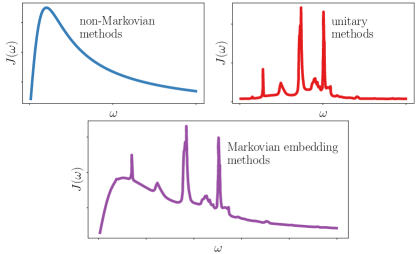
Figure 1: Current methods for simulating the quantum dynamics of excited states coupled to vibrational degrees of freedom target different types of environments. (Non-)Markovian methods are well-suited to describe continuous spectral densities (upper-left panel), while unitary methods work best for discrete spectral densities (upper-right panel), which capture long-memory effects in the environment. We introduce a pure-state unraveled hybrid-bath scheme using a Markovian-embedding (lower panel) to efficiently treat both types of environments.

The capability to simulate the ultrafast quantum dynamics of photophysical processes in complex molecules is essential to understanding phenomena such as exciton transfer and energy conversion, whose practical control is the foundation of the design of functional compounds with fascinating properties. Their possible applications range from tailored chemical catalysts to synthetic light-harvesting materials and solar cells with efficiencies beyond the Shockley-Queisser limit [1, 2, 3, 4, 5]. However, the corresponding computational problems involve the dynamics of excitonic states coupled to vibrational modes, each of which is a challenging problem on its own. Exploiting various simplifications, the computational task can be reduced to faithfully describe excitonic degrees of freedom (DOFs) representing electronic excited states, which are (non-locally) coupled to a manifold of vibrational DOFs. Here, especially the vibrational system of complex molecules poses various numerical challenges and there has been a great effort to deal with the exponential scaling of the computational complexity. In general, two conceptually different approaches were established. (i) A discretization of the vibrational DOFs is combined with selection rules to choose the most relevant modes, such that the unitary dynamics of the resulting, closed quantum system can be described using efficient state representations and integration schemes [6, 7, 8, 9, 10]. (ii) The excitonic DOFs are treated exactly while the vibrational DOFs are traced out and encoded in an effective environment. The complexity of the resulting, open quantum-system dynamics then mainly depends on the choice of the environment [11, 12]. The dynamics in the presence of memoryless, Markovian environments can be treated efficiently using Lindblad master quations[13, 14, 15, 16, 17]. Structured, non-Markovian environments introduce time-non-local correlations between system and environment, which increase the computational cost [18, 19, 20, 21, 22, 23, 24, 25, 26, 27, 28, 29] but are crucial to simulate the inherently mesoscopic vibrational systems of molecules, exhibiting long-time memory effects.

To efficiently simulate the quantum dynamics of both, coupled electronic and vibrational, as well as environmental DOFs, the decomposition of the many-body wavefunction into local tensors has proven to be an extremely fruitful approach[30, 31, 32, 33, 34, 35, 36, 37, 38]. The unitary evolution of excitonic states coupled to $\mathcal{O}(100)$ discrete vibrational DOFs is a remarkable milestone facilitating, for instance, the unbiased investigation of ultrafast photo-induced dynamics of large molecules [39, 40, 41]. Recently, wavefunction-based tensor network (TN) methods for open quantum-systems with both Markovian and non-Markovian environments have been developed [42, 43, 44] to describe continuous and smooth spectral densities.

However, these approaches leave a methodological gap, if the system’s spectral density contains both aspects, discrete peaks immersed into a smooth background. This situation, generated for instance by non-vanishing memory effects, is inevitable in realistic materials, such as organic semiconductors, which involve both dispersive modes with continuous spectral densities and local vibrational modes with sharp peaks. While in these cases the unitary approach would require a daunting amount of discrete vibrational modes, generic open-quantum system methods become unstable in the presence of discrete peaks [45]. To fill this gap, pseudomode approaches have been introduced in order to approximate the spectral density by introducing damped auxiliary modes [46, 22, 47, 48, 49] and solving the equations of motion for the density operator [50, 51]. Here, we propose a TN -based pure-state unraveled hybrid-bath (PS-HyB) scheme computing quantum trajectories in terms of matrix-product state (MPS) of an enlarged system with Markovian embedding, where both continuous and discrete contributions to the spectral density can be handled (see  Fig. 1). Simulating two paradigmatic examples, i.e., singlet fission in a three-state model with Debye spectral density, as well as finite-temperature exciton-dynamics in an Fenna–Matthews–Olson (FMO) complex with an additional sharp peak in the spectral density, we demonstrate that PS-HyB -MPS can efficiently capture the regime of long-time memory effects at significantly smaller computational cost than unitary methods, while it circumvents instabilities from a direct evolution of the density operator. This is achieved by exploiting recent advances for TN -representations of systems with large local Hilbert spaces, rendering a pure-state unravelling practically feasible, also in the presence of strong exciton-phonon couplings [52, 53, 40, 54, 55].

II Methodology

We aim to describe the dynamics of $L$ excitonic states, each interacting with a set of vibrational DOFs, acting as independent environments. For this system-environment partitioning, the spectral density $J^{I}(\omega)$ ($I=1,2,\dots L)$ is the key quantity encoding the relevant information about the coupling between excitonic and the vibrational DOFs. Our goal is to capture the general situation of a continuous background and discrete, sharp peaks describing long-time memory effects, as pictured in Fig. 1. For that purpose, we adopt a method called mesoscopic leads or extended reservoirs[22, 23, 24, 25, 26, 27, 28]. In this framework, the general idea is to approximate each bath spectral density $J^{I}(\omega)=\pi/2\sum_{k}|g^{I}_{k}|^{2}\delta(\omega-\omega_{k})$ by fitting it with $N^{I}$ Lorentzians:

$$J^{I}(\omega)=\sum_{m=1}^{N^{I}}\frac{\gamma^{I}_{m}\absolutevalue{g^{I}_{m}/2}^{2}}{(\omega-\omega^{I}_{m})+(\gamma^{I}_{m}/2)^{2}}\;,$$ (1)

where the couplings between excitonic and vibrational DOFs are given by $g^{I}_{m}=\sqrt{2J^{I}(\omega)\gamma^{I}_{m}/\pi}$, and we have introduced a discrete spacing $\gamma^{I}_{m}=\omega^{I}_{m+1}-\omega^{I}_{m}$. Each Lorentzian contributing to the spectral density can be represented by a harmonic oscillator with frequency $\omega^{I}_{m}$ coupled to a memoryless environment, where the spectral broadening is given by the potentially non-uniform discretization $\gamma^{I}_{m}$. This way, we can represent a continuous spectral density with sharp features by a set of $\sum_{I}N^{I}$ bosonic modes coupled to Markovian environments.

Let us now work with the explicit Hamiltonian for the combined excitonic and vibrational system

$$\hat{H}=\hat{H}_{\mathrm{exc}}+\hat{H}_{\mathrm{vib}}+\hat{H}_{\mathrm{ex-vib}}\;.$$ (2)

Here, $\hat{H}_{\mathrm{exc}}$ is an arbitrary excitonic Hamiltonian. In the following, we set $k_{B},\,\hbar=1$. The vibrational modes are described by harmonic oscillators with frequencies $\omega^{I}_{m}$: $\hat{H}_{\mathrm{vib}}=\sum_{m,I}\omega^{I}_{m}\hat{b}^{I\dagger}_{m}\hat{b}^{I}_{m}$, where $\hat{b}^{I(\dagger)}_{m}$ are the bosonic annihilation (creation) operators. The interaction between excitons and vibrational modes takes the form $\hat{H}_{\mathrm{ex-vib}}=\sum_{m,I}g^{I}_{m}\hat{n}^{I}(\hat{b}^{I}_{m}+\hat{b}^{I\dagger}_{m})/\sqrt{2}$.

Upon introducing a sufficient number of oscillators $N^{I}$, the dynamics of the combined system obeys the Lindblad equation [13, 14]

$$\frac{\mathrm{d}\hat{\rho}}{\mathrm{d}t}=\mathcal{L}(\hat{\rho})=-i\commutator{\hat{H}}{\hat{\rho}}+\sum_{I}\mathcal{D}^{I}(\hat{\rho})\;.$$ (3)

The sum on the right-hand side models the interaction of the system with a Markovian environment. In our case, these terms describe the thermalization of each vibrational subsystem $I$ via the Davies map [56, 57]

$$\mathcal{D}^{I}(\hat{\rho})=\sum_{m=1}^{N^{I}}\gamma^{I}_{m}\left[f^{I}_{m}\mathcal{D}(\hat{\rho},\hat{L}_{1})+(1+f^{I}_{m})\mathcal{D}(\hat{\rho},\hat{L}_{2})\right],$$ (4)

where the thermalization rate is proportional to the spacing and $f^{I}_{m}(\beta)=1/(\exp(\beta\omega^{I}_{m})-1)$ is the Bose-Einstein distribution function at inverse temperature $\beta$. Here, we introduced the dissipator

$$\mathcal{D}(\hat{\rho},\hat{L}_{l})=\hat{L}^{\phantom{\dagger}}_{l}\hat{\rho}\hat{L}^{\dagger}_{l}-\frac{1}{2}\left\{\hat{L}^{\dagger}_{l}\hat{L}^{\phantom{\dagger}}_{l},\hat{\rho}\right\}\;;$$ (5)

specifying the couplings to the environment via the jump operators $\hat{L}_{1}=\hat{b}^{I\dagger}_{m}$ and $\hat{L}_{2}=\hat{b}^{I}_{m}$.

For a large number of bath modes $N^{I}$, the dissipative evolution of the excitonic subsystem Eq. 3 becomes equivalent to the unitary evolution with discretized bath spectral densities [58], described for instance via a chain mapping [28]. We will show the mesoscopic leads approach to be numerically much more efficient when solving the dynamics using TN methods. This is based on the observation that one obtains the unitary case from taking the zero-broadening limit of Eq. 3. In fact, when $J(\omega)$ is continuous and smooth (upper left panel of Fig. 1) a large number of discrete modes would be required to accurately fit $J(\omega)$. Moreover, unitary dynamics suffer from severe finite-size errors caused by the scattering of excitations at the systems’ boundaries, which limits the reachable simulation time [28].

Nonetheless, compared to unitary time evolution, Lindblad dynamics pose challenges to numerical treatments not only because of the dimension but also because the truncation of a mixed state requires particular care [59, 60]. It is thus convenient to resort to so-called pure-state unravelings, which consist of reconstructing the Lindblad dynamics from an ensemble of stochastic pure-state time evolutions. Different pure-state unraveling schemes, such as quantum state diffusion (QSD) [61] and the quantum jumps (QJ) [16, 17] approach have been developed. Here, we apply the QJ scheme, which is the more widely used variant due to its good stability and convergence properties. The starting point for the QJ scheme is to rewrite Eq. 3 in terms of jump operators $\hat{L}^{(\dagger)}_{l}$

$$\frac{\mathrm{d}\hat{\rho}(t)}{\mathrm{d}t}=-i\commutator{\hat{H}_{\mathrm{eff}}}{\hat{\rho}(t)}+\sum_{l}\hat{L}^{\phantom{\dagger}}_{l}\hat{\rho}(t)\hat{L}^{\dagger}_{l}\;,$$ (6)

where $\hat{H}_{\mathrm{eff}}=\hat{H}-i/2\sum_{l}\hat{L}^{\dagger}_{l}\hat{L}^{\phantom{\dagger}}_{l}$ is an effective, non-Hermitian Hamiltonian. If the initial state is pure ($\hat{\rho}(0)=\ket{\Psi(0)}\bra{\Psi(0)}$) the first term of Eq. 14 describes a simple (non-unitary) Schrödinger evolution. The action of the second term can be mapped to the stochastic application of $\hat{L}_{l}$ to a pure state. This is achieved by introducing a collection of random numbers defining trajectories $q(t)$ (see for instance 16) such that at any time $t$ the ensemble average $\mathcal{E}$ over many pure-state evolutions yields the Lindblad-evolved density matrix $\mathcal{E}\left[\ket{\Psi(t)_{q}}\bra{\Psi(t)_{q}}\right]=\hat{\rho}(t)$. Usually, one avoids computing the density matrix explicitly and evaluates the expectation value of an observable of interest directly as $\langle\hat{O}\rangle(t)=\mathcal{E}[\bra{\Psi(t)_{q}}\hat{O}\ket{\Psi(t)_{q}}]$.

We represent the excitonic-vibronic system as a MPS [6, 8]. This allows us to employ efficient truncation schemes for $\ket{\Psi}$ that are controlled by the bond dimension and/or the truncated weight. Representing the vibrational modes as an MPS is an arduous task because one has to truncate the formally infinite bosonic Hilbert space. Moreover, the interaction Hamiltonian breaks the $U(1)$ symmetry for the bosonic excitations. Both challenges can be addressed by the projected-purification (PP) method [52, 53], which was successfully applied to simulate unitary photo-induced dynamics in different setups [40, 54, 55]. To calculate the time-evolution of an MPS, one of the most efficient methods is the time-dependent variational principle (TDVP) [62, 9, 10], which is based on the Dirac-Frenkel variational principle [63]. For bosonic degrees of freedom, we choose the single-site variant of TDVP with a local subspace expansion [64, 65], which exhibits the computationally most favorable scaling. It combines single-site TDVP updates with local basis expansions, increasing the states’ bond dimension. In this way, it captures the spread of correlations during the time evolution, while the dominating contractions scale only quadratically in the cutoff dimension of the local bosonic Hilbert spaces. Finally, in order to describe vibrational environments at finite temperatures, we perform a thermofield doubling of the bosonic system and map the bosonic thermal state to the vacuum via a Bogoljubov transformation [66].

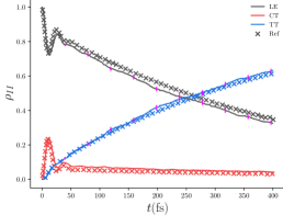
(a)

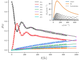
(b)

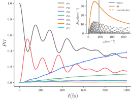
(c)

Figure 2: Dynamics of the excitonic populations $\rho_{II}=\braket{I}{\hat{\rho}}{I}$ for a three-state model of SF LABEL:sub@fig:example:sf at $T=0\mathrm{K}$ and a photo-excited FMO complex at $T=300\mathrm{K}$ LABEL:sub@fig:example:fmo:300k and $T=77\mathrm{K}$ LABEL:sub@fig:example:fmo:77k+peak, using a Debye spectral density, which in LABEL:sub@fig:example:fmo:77k+peak is extended by a vibrational mode of the FMO pigments. The solid lines are obtained using PS-HyB -MPS with a QJ pure state unravelling using $1000$ independent trajectories; error bars are shown only every $50\mathrm{fs}$ LABEL:sub@fig:example:sf and $100\mathrm{fs}$ LABEL:sub@fig:example:fmo:300k, LABEL:sub@fig:example:fmo:77k+peak. Reference values are denoted by crosses, extracted from Ref. 34 for LABEL:sub@fig:example:sf and Ref. 12 for LABEL:sub@fig:example:fmo:300k. In the insets, we display the fitting of the spectral density at the example of FMO. We find excellent agreement with the reference data using a rather small number of Lorentzians $N^{I}=10$ for LABEL:sub@fig:example:sf and $N^{I}=19$ for LABEL:sub@fig:example:fmo:300k, LABEL:sub@fig:example:fmo:77k+peak.

III Example 1: Singlet fission

In order to benchmark the capability of PS-HyB -MPS to reduce the necessary complexity of a faithful description of vibrational subsystems, we first studied a paradigmatic, minimal model for singlet fission at zero temperature [34, 31, 54]. The excitonic part of the Hamiltonian consists of $L=3$ excitonic states usually referred to as the (i) locally excited (LE), (ii) charge transfer (CT), and (iii) two-triplet (TT) states. Each state is coupled to its own bath of harmonic oscillators characterized by a Debye spectral density

$$J^{D}(\omega)=\frac{2\lambda\omega\omega_{c}}{(\omega^{2}+\omega_{c}^{2})}\;.$$ (7)

We set $\lambda=807\mathrm{cm}^{-1}$, $\omega_{c}=1452\mathrm{cm}^{-1}$ and draw the explicit model parameter of $\hat{H}_{\mathrm{exc}}$ from [34]. The details on the numerical implementation together with a convergence analysis can be found in Apps. A, B and C. Following Sec. II, for each excitonic state we fit the corresponding spectral density $J^{D}(\omega)$ and we found $N^{I}=10$ vibrational modes to be sufficient to faithfully reproduce $J^{D}(\omega)$. At $t=0$, we prepared the excitonic system in the LE state and the vibrational environment in the $T=0\mathrm{K}$ vacuum state. Choosing a timestep $\delta t=5\;\mathrm{fs}$ and a cutoff dimension $d=16$ for the bosonic sites, we evaluated the time-dependent excitonic populations, averaging over $1000$ independent trajectories. In Fig. 2a we show the resulting dynamics (solid lines, error bars indicated every $50\mathrm{fs}$) compared to reference data (crosses) extracted from Ref. 34. We find an excellent agreement also at very long simulation times using only $N^{I}=10$ bosonic modes per excitonic state, which should be compared to $N^{I}=61$ modes per excitonic state used in the unitary time-evolution scheme of Ref. 34. Small deviations can be attributed to the number of sample trajectories, which is discussed in more detail in App. B.

IV Example 2: Light-harvesting complex

Simulating complex excitonic dynamics at finite temperatures is an even more challenging problem, in particular when using wavefunction-based methods. As a second example, we therefore studied the photo-induced dynamics of the FMO -complex at finite temperature. It is a pigment-protein complex found in green sulfur bacteria, which is involved in the early stages of photosynthesis [67].

Following the literature, we used $L=7$ excitonic states for the FMO complex. Each state is coupled to an independent vibrational environment [12], which we initialized at a finite temperature [66] (see App. D). The excitonic Hamiltonian is given by

$$\hat{H}_{\mathrm{exc}}=\sum_{I,J=1}^{7}t_{IJ}\ket{I}\bra{J}\;,$$ (8)

where we adopted the couplings $t_{IJ}$ from Ref. 12. The standard approach to describe the vibrational system is by assuming a Debye spectral density Eq. 7, which we fit with $N^{I}=19$ Lorentzians per vibrational environment. We extend this approach by adding a sharp peak at a frequency $\omega_{0}=29\mathrm{cm}^{-1}$, which is generated from a vibrational mode of the individual pigments. We emphasize that this modification introduces long-time memory effects in the environment that can significantly alter the photo-induced dynamics. Moreover, previous studies which used a non-Markovian description of the environments, only considered finite broadenings [12] of this mode, drastically reducing memory-effects. We performed simulations of the photo-induced dynamics at the practically relevant temperatures $T=77\mathrm{K}$ and $300\mathrm{K}$ measuring the time-dependent exciton population, starting from an initial exciton configuration $n_{1}=1,n_{I>1}=0$, and using $1000$ independent trajectories.

In Fig. 2b we show the resulting dynamics for the case of a pure Debye spectral density, i.e. without the additional peak at $\omega_{0}$, at $T=300\mathrm{K}$. The solid lines represent the time-dependent excitonic state occupations and the error bars are now indicated every $100\mathrm{fs}$. We again find excellent agreement with the reference data (crosses), reaching a very long simulation time of $1\mathrm{ps}$. In the inset, we show the quality of the fit of the Debye spectral density Eq. 7, using $N^{I}=19$ Lorentzians. We checked that the small oscillations around the exact shape of $J^{D}(\omega)$ have no impact on the obtained dynamics.

Taking into account the additional $\delta$-peak in $J^{D}(\omega)$, we performed computations at $T=77\mathrm{K}$. The resulting, time-dependent excitonic occupations are depicted in Fig. 2c. Note the additional $\delta$-peak in the spectral density indicated by the green dashed line of the inset. The effect of the long-term memory induced by the dissipationless additional mode immediately translates into the excitonic dynamics. Compared to the Debye-only case, we find long-lived oscillations in the excitonic occupations, with an increased coherence time compared to Ref. 12, due to the exact treatment of the $\delta$-peak.

V Benchmark

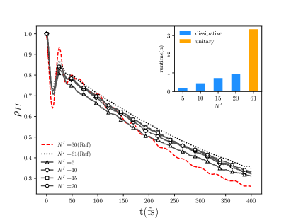
Figure 3: Convergence of the LE population $\braket{\mathrm{LE}}{\hat{\rho}}{\mathrm{LE}}$ for the SF -example obtained from unitary evolution using $N^{I}=30$ (red dashed) and $N^{I}=61$(black dotted) modes, representing the most relevant vibrational modes [68] compared to the dynamics obtained from PS-HyB -MPS. For the case of $N^{I}=30$ modes, the unitary dynamics exhibit stronger oscillations caused by finite-size effect. Note that using PS-HyB -MPS, the unitary dynamics with $N^{I}=61$ modes is well-reproduced but with a significantly smaller number of bosonic modes $N^{I}=10$. In the inset, we show a runtime comparison of the unitary dynamics (red bar) with PS-HyB -MPS (blue bars). The computational speed up is nearly an order of magnitude, due to the drastically reduced number of bosonic modes required.

Besides ensuring the consistency of PS-HyB -MPS, we also performed benchmark computations to compare the efficiency of PS-HyB -MPS to that of standard, unitary dynamics, here at the example of SF Sec. III. In Fig. 3 we show the dynamics of the LE state (solid lines), computed using different numbers of $N^{I}=5,10,15,20$ Lorentzians to approximate Eq. 7. The unitary dynamics was calculated taking into account $N^{I}=30$ (dashed line) and $N^{I}=61$ (dotted line) relevant vibrational modes where it has been shown that $N^{I}=61$ is required to faithfully describe the excitonic dynamics [68]. Due to the discrete nature of the vibrational environment in the unitary approach, finite-size effects are observed that translate to stronger oscillations in the initial dynamics. Nevertheless, PS-HyB -MPS reproduces both, the initial and long-time dynamics but with a much smaller number of bosonic modes. This translates into a significant reduction of the runtime, which is shown in the inset. Using only $N^{I}=10$ modes, the observed computational speedup is a factor of $\sim 7.5$. We also note that the finite lifetime of the bosonic excitations generated by the dissipative evolution in PS-HyB continuously decreases both, the bond and effective bosonic Hilbert space dimensions, in the scope of the dynamics.

Summary and Outlook

In this work we introduced PS-HyB -MPS, a method that allows us to efficiently describe the influence of both continuous and discrete vibrational quantum baths on exciton dynamics. To this end, we combine a Markovian-embedding scheme with a pure-state unraveling and state-of-the-art tensor network techniques to represent and evolve bosonic baths with very large Hilbert space dimensions. PS-HyB -MPS is capable of describing both short-and long-time memory effects in exciton dynamics at finite temperatures while requiring a much smaller amount of bosonic modes compared to commonly used unitary descriptions. The resulting reduction in computational complexity translates into significantly lower numerical costs; for instance, we obtain a speedup of nearly an order of magnitude for a paradigmatic model of singlet fission. We believe that PS-HyB -MPS will be a valuable tool to tackle the description of intricated excitonic dynamics in vibrational environments, opening the possibility to describe mesoscopic environments efficiently by using wavefunction-based time-evolution schemes. Moreover, the prospect of overcoming the current limitation of independent vibronic baths using non-Markovian descriptions of the environment (see App. E) opens the possibility to increase the computational efficiency of more complex problems, such as photo-induced excitonic dynamics in the presence of coupled vibrational modes.

Appendix A Numerical details

Table 1: Parameters of 19 optimized modes for FMO

$\omega/\mathrm{eV}$	$\kappa/\mathrm{eV}$	$\gamma/\mathrm{eV}$
2.30099e-03	6.88515e-04	9.50196e-04
3.28506e-03	9.58415e-04	1.21617e-03
4.33189e-03	1.20018e-03	1.47447e-03
5.47123e-03	1.43038e-03	1.74525e-03
6.72464e-03	1.65352e-03	2.04209e-03
9.67419e-03	2.08386e-03	2.77137e-03
8.11579e-03	1.87114e-03	2.37871e-03
1.14380e-02	2.29190e-03	3.24048e-03
1.34576e-02	2.49578e-03	3.81300e-03
1.57994e-02	2.69633e-03	4.52527e-03
1.85530e-02	2.89496e-03	5.42731e-03
2.18399e-02	3.09376e-03	6.58909e-03
2.58265e-02	3.29575e-03	8.10986e-03
3.07445e-02	3.50484e-03	1.01299e-02
3.69172e-02	3.72623e-03	1.28428e-02
4.47954e-02	3.96608e-03	1.64867e-02
5.49886e-02	4.23097e-03	2.12190e-02
6.82436e-02	4.51903e-03	2.64008e-02
8.52510e-02	4.74554e-03	2.68574e-02

In this appendix, we provide additional details on the numerical methods used in the main text. We represent the state of the excitonic and of the vibrational degrees of freedom as an MPS [8]. We use the PP mapping  [52] for the vibrational modes, which allows us to determine the optimal local dimensions for the vibrational modes at every time evolution step. For all results presented in the main text, we allowed for a maximum local dimension $d_{\mathrm{max}}$ of $=16$. For the time evolution, we used the TDVP algorithm [62, 9]. Specifically, we employed the local subspace expansion time-dependent variational principle (LSE-TDVP) [64, 65], which is very efficient, especially for systems with large local dimensions, like the vibrational modes in our case. This consists of single-site TDVP steps with some maximal bond dimension $m$ alternated by expansions that increase the state’s bond dimension by $m_{e}$. Unless otherwise stated, we set $m=50$ and $m_{e}=10$. For the TN calculations, we used the SyTen toolkit [72, 73].

We unraveled the Lindblad equation using the QJ method (see also App. C) with a time step of $dt=5$ fs and either $N_{\mathrm{trajs}}=500$ or $N_{\mathrm{trajs}}=1000$ trajectories (see the figure captions). The QJ method was implemented in evos, a Python package for open quantum system dynamics that uses SyTen as the backend. All computations were performed on an Intel Xeon Gold 6130 CPU (2.10GHz) with 16 threads. For all singlet fission calculations, we fitted the spectral density using an equally spaced discretization. Instead, for the FMO dynamics we found it more convenient to use a non-equally-spaced discretization, as shown in LABEL:table:7x19.

Appendix B Singlet fission with different number of trajectories

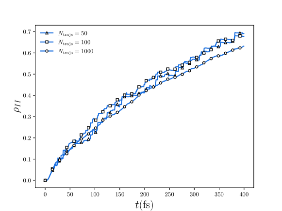
Figure 4: Population of TT state in Markovian embedding dissipative dynamics(equally spaced $N^{I}=10$) with different numbers of trajectories.

In the main text, we computed the time evolution of a singlet fission model using Markovian embedding dissipative dynamics. We showed that accurate results for the dynamics can be obtained by replacing a large closed system ($N^{I}=61$) with a much smaller open system ($N^{I}=10$). The disadvantage of the dissipative approach is that one time evolution is replaced by an ensemble of trajectories. However, we argue that this is only a minor disadvantage for the following reasons:

• Although reproducing smooth dynamics can require up to $\mathcal{O}(1000)$ trajectories, a very small number of trajectories already suffices to reproduce the qualitatively correct dynamics, i.e. the generation of TT state( see Fig. 4). Therefore, a quick estimation of the dynamics can be easily achieved using this scheme instead of performing a fine discretization for each subregion of the spectrum [34, 31].

• Each quantum trajectory is completely independent of the others. This enables a trivial, perfect parallelization over trajectories which enhances and simplifies high-performance computations.

• For isolated many-body, strongly-correlated systems with bosonic DOFs, TDVP requires large bond dimensions $m$ and large local dimensions $d$. Instead, as we demonstrate in App. C, dissipatively coupling the vibrational modes to a bath suppresses both the bond dimension and the physical dimension.

Appendix C Comparing Markovian embedding and unitary evolution

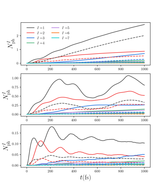
Figure 5: Total phononic occupation in the bath of each site($N_{ph}^{I}=\sum_{k}\langle\hat{b}^{I\dagger}_{k}b^{I}_{k}\rangle$) using equally spaced $N^{I}=30$ unitary evolution (upper panel), equally spaced $N^{I}=6$ unitary evolution (middle panel) and equally spaced $N^{I}=6$ Markovian embedding scheme (lower panel). The phononic occupations of the unitary evolutions are larger than the ones of the Markovian embedding scheme by one order of magnitude. Here, solid lines indicate positive-frequency modes and dashed lines for negative-frequency modes in the thermofield doubling scheme [66] (see App. D).

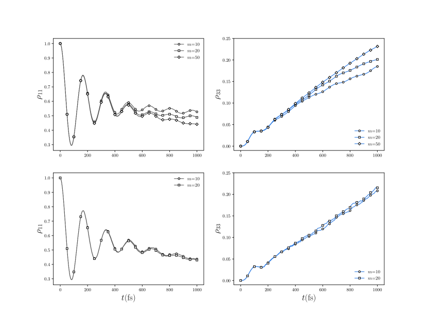
Figure 6: Bond dimension $m$ convergence of the unitary evolution (upper) and Markovian embedding (lower) using equally spaced $N^{I}=30$. We show the populations of site $1$ (black, left panels) and site $3$ (blue, right panels). The local dimensions of dissipative dynamics are fixed to $d=2$.

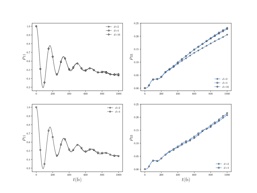
Figure 7: Local dimension $d$ convergence of the unitary evolution (upper) and Markovian embedding (lower) using equally spaced $N^{I}=30$. We show the populations of site $1$ (black, left panels) and site $3$ (blue, right panels). The bond dimensions of dissipative dynamics are fixed to $m=10$.

In this section, we explain similarities and differences between unitary and (non-unitary)Markovian embedding schemes based on MPS we performed in the main text. First, they share the equivalent decomposition of a continuous spectral density into discrete modes. For simplicity, we assume the spectral densities $J^{I}(\omega)$ are discretized into $N^{I}$ modes, equally spaced by $\Delta\omega$. The $k$-th mode evolves with frequency $\omega_{k}$ and couples to the excitonic system via $g_{k}^{I}\hat{n}^{I}(\hat{b}^{I}_{k}+\hat{b}^{I\dagger}_{k})/\sqrt{2}$. In the unitary scheme, the system and these discrete modes together form a large closed system where the coupling coefficients are

$$g^{I}_{k}=\sqrt{\frac{2}{\pi}J^{I}(\omega_{k})\Delta\omega}.$$ (9)

In the Markovian embedding scheme, the mesoscopic leads method [22, 23, 24, 25, 26, 27, 28] decomposes the spectral densities into Lorentzians (with center $\tilde{\omega}_{m}$ and width $\gamma$). In analogy to Eq. 9, the coupling between an excitonic mode $I$ and a vibrational mode with frequency $\tilde{\omega}_{m}$ is given by

$$\tilde{g}^{I}_{m}=\sqrt{\frac{2}{\pi}J^{I}(\tilde{\omega}_{m})\gamma},$$ (10)

where the Lorentzian widths are chosen to be $\gamma=\tilde{\omega}_{m+1}-\tilde{\omega}_{m}=\Delta\tilde{\omega}$. The vibrational system is embedded in Markovian environments characterized by a dissipation strength $\gamma$. Therefore, if the same discrete frequencies are chosen, these two schemes evolve the same excitonic-vibrational system either unitarily as a closed system where the rest of the continuous bath is completely ignored (namely, the broadening is completely absorbed into the discrete peak) or as an open system with the Markovian embedding.

In the following, we compare the unitary dynamics to the dissipative Markovian-embedding dynamics unraveled with QJ. The evolution of a closed system with initial pure state $|\Psi(0)\rangle$ obeys the Schrödinger equation

$$\frac{\partial}{\partial t}|\Psi(t)\rangle=-i\hat{H}|\Psi(t)\rangle,$$ (11)

where $\hat{H}$ is the Hermitian Hamiltonian of the enlarged system discussed above (exctions and vibrational modes). The induced time-dependence is given by

$$|\Psi(t+\delta t)\rangle=e^{-i\hat{H}\delta t}|\Psi(t)\rangle,$$ (12)

and in practical numerical computations, one typically splits the unitary time evolution operator into several time steps

$$|\Psi(t)\rangle=e^{-i\hat{H}\delta t}\cdots e^{-i\hat{H}\delta t}|\Psi(0)\rangle.$$ (13)

In the Markovian embedding scheme, the evolution of the enlarged system obeys the Lindblad master equation

$$\frac{\partial\hat{\rho}(t)}{\partial t}=-i\commutator{\hat{H}_{\mathrm{eff}}}{\hat{\rho}(t)}+\sum_{l}\hat{L}^{\vphantom{\dagger}}_{l}\hat{\rho}(t)\hat{L}^{\dagger}_{l},$$ (14)

where $\hat{H}_{\mathrm{eff}}=\hat{H}-i/2\sum_{l}\hat{L}^{\dagger}_{l}\hat{L}_{l}\equiv\hat{H}-i\hat{H}^{\prime}$. The QJ method unravels the evolution of the density matrix $\hat{\rho}(t)$ into an ensemble of quantum trajectories [16]. Each trajectory follows a non-unitary evolution, accompanied by quantum jumps happening at random times. At every timestep, with a probability of $1-\delta p$, a trajectory either evolves under a non-Hermitian Hamiltonian

$$|\Psi(t+\delta t)\rangle=e^{-i\hat{H}_{\mathrm{eff}}\delta t}|\Psi(t)\rangle,$$ (15)

or undergoes a jump with a probability $\delta p$

$$|\Psi(t+\delta t)\rangle=\hat{L}_{l}|\Psi(t)\rangle.$$ (16)

Here, the probability of having a quantum jump is determined by the norm loss during non-unitary evolution

$$\delta p=1-\langle\Psi(t)|e^{+i\hat{H}^{\dagger}_{\mathrm{eff}}\delta t}e^{-i\hat{H}_{\mathrm{eff}}\delta t}|\Psi(t)\rangle.$$ (17)

Up to first order in $\delta t$, the norm loss can be decomposed as

$$\delta p\approx\delta t\langle\Psi(t)|i(\hat{H}_{\mathrm{eff}}-\hat{H}_{\mathrm{eff}}^{\dagger})|\Psi(t)\rangle=\delta t\sum_{l}\langle\Psi(t)|\hat{L}^{\dagger}_{l}\hat{L}_{l}|\Psi(t)\rangle\equiv\sum_{l}\delta p_{l}.$$ (18)

Note that the Hermitian part of the effective Hamiltonian $\hat{H}$ is nothing but the Hamiltonian of the closed system in a unitary scheme. At zero temperature, the jump operators used in the mesoscopic leads method are

$$\hat{L}_{l}=\sqrt{\gamma}\;\hat{b}_{k}^{I}$$ (19)

where $\gamma$ is the decay rate of the vibrational modes. Thus, the probability of each decay channel is proportional to its phononic occupation

$$\delta p_{l}=\gamma\delta t\langle\Psi(t)|\hat{b}^{I\dagger}_{k}\hat{b}^{I}_{k}|\Psi(t)\rangle.$$ (20)

To compare with the unitary evolution more straightforwardly, we trotterize the evolution of $\hat{H}_{\mathrm{eff}}$ into the evolution of Hermitian $\hat{H}$ and anti-Hermitian part $-i\hat{H}^{\prime}$:

$$|\Psi(t+\delta t)\rangle=e^{-i\hat{H}_{\mathrm{eff}}\delta t}|\Psi(t)\rangle\approx e^{-\hat{H}^{\prime}\delta t}e^{-i\hat{H}\delta t}|\Psi(t)\rangle.$$ (21)

Following 13, the evolution is split into time steps

$$|\Psi(t)\rangle=e^{-\hat{H}^{\prime}\delta t}e^{-i\hat{H}\delta t}\cdots e^{-\hat{H}^{\prime}\delta t}e^{-i\hat{H}\delta t}|\Psi(0)\rangle.$$ (22)

22 can be seen as an alternating sequence of imaginary evolution steps $e^{-\hat{H}^{\prime}\delta t}$ and real-time evolution steps $e^{-i\hat{H}\delta t}$. The imaginary time evolution can be expressed in terms of jump operators 19

$$e^{-\hat{H}^{\prime}\delta t}=e^{-\gamma\delta t/2\sum_{k}\hat{b}^{I\dagger}_{k}\hat{b}_{k}^{I}}.$$ (23)

23 indicates an exponential suppression of the phononic occupation with strength $\gamma\delta t$ at each unitary (real) time evolution step (see Fig. 5). Such suppression results in a loss of norm 17 and can lower the local dimensions (Fig. 7) and the bond dimensions (Fig. 6) of TDVP calculations. Thus, an expensive unitary evolution can be substituted by much cheaper evolutions of multiple trajectories. Note that at finite temperatures, the creation operators are also the jump operators in the mesoscopic leads method. However, the prefactor of the annihilation jump operators is always larger than that of the creation operators, typically resulting in a decrease in the bond dimension and the local dimension compared to the unitary evolution at any temperature.

Appendix D Finite temperature: Thermofield doubling vs unraveling

For the simulations of the exciton dynamics of the FMO complex discussed in the main text, we initialized the system in a tensor product state between a pure excitonic state and a thermal state of the vibrational system

$$\hat{\rho}(0)=\ket{\psi(0)}_{\mathrm{ex}}\bra{\psi(0)}_{\mathrm{ex}}\otimes\hat{\rho}^{\beta}_{\mathrm{vib}}.$$ (24)

In order to represent the mixed state $\hat{\rho}^{\beta}_{\mathrm{vib}}$ as an MPS, there are different possible strategies: for instance to double the Hilbert space for the vibrational degrees of freedom or to unravel the thermal state.

The first method, known as thermofield doubling, is widely used in MPS calculations [74, 8]. For Hamiltonians as the one considered in the main text, where the vibrational modes are described by independent harmonic oscillators and the coupling to the excitonic system is linear, de Vega and Bañuls in Ref. 66 introduced a useful trick that simplifies the calculations. In short, the idea is to introduce a new set of bosonic operators $\hat{a}_{k}$, linked to the original operators $\hat{b}_{k}$ by a unitary transformation, that annihilates the thermal state $\hat{\rho}^{\beta}_{\mathrm{vib}}$. By transforming the Hamiltonian to the new basis, the thermal state can be represented as a vacuum state. This not only decreases the bond dimension of the initial state, but most importantly it reduces the number of quantum jumps from the environment to the vibrational modes, strongly improving the convergence of the  QJ method, as shown in Fig. 8.

The second method consists in unraveling the thermal state $\hat{\rho}^{\beta}_{\mathrm{vib}}=\sum_{k}p(k)\ket{\psi^{k}}_{\mathrm{vib}}\bra{\psi^{k}}_{\mathrm{vib}}$, by sampling pure states $\ket{\psi^{k}}_{\mathrm{vib}}$ according to the probability distribution $p(k)$. This additional sampling of the initial state, which adds to the sampling of the QJ method, increases the total number of trajectories required to converge the simulations. Since the vibrational degrees of freedom are described by independent harmonic oscillators, the thermal state in Eq. 24 can be written as

$$\hat{\rho}^{\beta}_{\mathrm{vib}}=e^{-\beta\hat{H}_{\mathrm{vib}}}/Z=e^{-\beta\sum_{I,m}\omega^{I}_{m}\hat{n}^{I}_{m}}/Z=\prod_{I,m}e^{-\beta\omega^{I}_{m}n^{I}_{m}}/Z,$$ (25)

where $\hat{n}^{I}_{m}$ is the bosonic number operator and $Z=\Tr(e^{-\beta\hat{H}_{\mathrm{vib}}})$ is the partition function, and thus the sampling of the full thermal state factorizes into a simple sampling from the Boltzmann distribution for each mode.

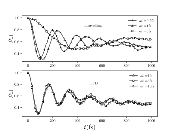
Figure 8: Thermal state unraveling vs. thermofield doubling (TFD). The population of the first FMO excitonic site at 77K was computed using Markovian embedding dissipative dynamics with 50 trajectories. The finite temperature is treated either by unraveling the thermal equilibrium state (upper panel) or via TFD (lower panel).

In Fig. 8 we compare the performance of the thermofield doubling against the unraveling of the thermal state. We simulate the occupation of the first excitonic site of the FMO at $77K$ using 50 trajectories for different timesteps $dt$. It can be seen that while the thermofield method yields good results for $dt=5$fs the unraveling method is not converged even for a ten times smaller timestep. This comes from the fact that at $77K$ the probability of quantum jumps happening between the thermal environment and the vibrational modes is much higher than at zero temperature, and the increased number of jumps strongly slows down the real-time evolution. Therefore, the mapping of the thermal state to a vacuum state [66] is crucial.

Appendix E Markovian embedding vs non-Markovian methods

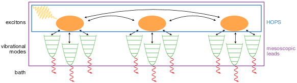
Figure 9: Two equivalent descriptions of exciton dynamics in a vibrational environment. Non-Markovian methods like HOPS consider only the exciton subsystem explicitly, while Markovian-embedding techniques as the mesoscopic leads method include also the vibrational modes.

In the main text, we have described the photo-induced dynamics of exciton systems strongly coupled to vibrational degrees of freedom by applying the Markovian-embedding-based mesoscopic leads method [22, 23, 24, 25, 26, 27, 28].

This consists of evolving the full excitonic-vibrational Hamiltonian exactly and damping the vibrational modes through a Lindblad dissipator. Here we outline an alternative, non-Markovian description and explore its connection to the mesoscopic leads method.

Instead of evolving the combined excitonic-vibronic state $\ket{\Psi}$ with the full Hamiltonian

$$\hat{H}=\hat{H}_{\mathrm{ex}}+\hat{H}_{\mathrm{vib}}+\hat{H}_{\mathrm{ex-vib}},$$ (26)

non-Markovian techniques allow us to deal directly only with $\hat{H}_{\mathrm{ex}}$ and consider the impact of the vibrational modes implicitly. The two possible system-environment bipartitions are shown in Fig. 9 For the sake of simplicity, let us consider the interaction Hamiltonian studied in the main text (although more general interactions are possible [21]):

$$\hat{H}_{\mathrm{ex-vib}}=\sum_{m,I}g^{I}_{m}\hat{n}^{I}(\hat{b}^{I}_{m}+\hat{b}^{I\dagger}_{m})/\sqrt{2},$$ (27)

where $g$ is the coupling strength, $\hat{n}$ is the excitonic number operator, and $\hat{b}^{\dagger}$ ($\hat{b}$) creates (annihilates) one vibrational mode. Differently from the mesoscopic leads approach, one describes the system-bath interaction by working in the time domain and considering the bath correlation function

$$\alpha^{I}(t-t^{\prime})=\int_{0}^{\infty}\mathrm{d}\omega J^{I}(\omega)\left[\coth(2\beta\omega)\cos(\omega(t-t^{\prime}))-i\sin(\omega(t-t^{\prime}))\right].$$ (28)

Here $J^{I}(\omega)$ is the frequency-dependent bath spectral density, the superscript $I$ labels the different baths, and $\beta$ is the inverse bath temperature. Instead of of fitting $J^{I}(\omega)$ with Lorentzians, we approximate $\alpha^{I}(t-t^{\prime})$ with a sum of complex exponentials, for instance via the Laplace-Pade method [75], as:

$$\alpha^{I}(t-t^{\prime})\approx\sum_{m}^{N}g^{I}_{m}e^{\gamma^{I}_{m}\absolutevalue{t-t^{\prime}}-i\omega^{I}_{m}(t-t^{\prime})},$$ (29)

where $\gamma$ and $\omega$ are the damping rate and the vibrational frequency, respectively.

In the following, we will denote a pure state on the combined exciton-phonon system by $\ket{\Psi}$ and for the excitons only with $\ket{\psi}$. In analogy to the Markovian case [61], it is possible to formulate a stochastic equation of motion for pure-state trajectories $q$ (see main text), so that the ensemble average

$$\mathcal{E}[\ket{\psi^{q}(t)}\bra{\psi^{q}(t)}]=\hat{\rho}^{\mathrm{ex}}(t)$$ (30)

yields the correct time-evolved mixed state $\hat{\rho}^{\mathrm{ex}}$ for the excitons.

Here, $z(t)$ is a time-dependent complex colored noise with mean zero and correlations $\mathcal{E}[z(t)z^{*}(t^{\prime})]=\alpha(t-t^{\prime})$ and $\mathcal{E}[z(t)z(t^{\prime})]=0$ [76]. The time evolution for each trajectory is described by the so-called non-Markovian quantum state diffusion (NMQSD)

$$\partial_{t}\ket{\psi(t)}=-i\hat{H}_{\mathrm{ex}}\ket{\psi(t)}+\sum_{m,I}g^{I}_{m}z^{I*}_{m}(t)\hat{n}^{I}\ket{\psi(t)}-\sum_{m,I}g^{I}_{m}\hat{n}^{I}\int_{0}^{t}\mathrm{d}t^{\prime}\alpha^{I*}_{m}(t-t^{\prime})\frac{\delta\ket{\psi(t)}}{\delta z^{I*}_{m}(t^{\prime})},$$ (31)

where $\delta/\delta z^{I*}_{m}$ indicates a functional derivative. In practice, solving this equation directly is unfeasible because the third term is time non-local.

An efficient strategy for solving Eq. 31 was put forward by Suess, Eisfeld, and Strunz, who introduced the HOPS method [21]. The main idea of HOPS consists of approximating the time non-local  Eq. 31 with a hierarchy of time-local equations, which are simpler to solve. In [43, 44], the authors showed that these hierarchies can be mapped to bosonic modes, facilitating their representation as MPS. For every trajectory $q$, the time evolution for the state on the combined excitonic-auxiliary moded $\ket{\Psi}$ reduces to

$$\partial_{t}\ket{\Psi(t)}=\hat{H}^{q}_{\mathrm{eff}}(t)\ket{\Psi},$$ (32)

where $\hat{H}^{q}_{\mathrm{eff}}(t)$ is a non-Hermitian, time-dependent effective Hamiltonian [43, 42].

In [17], a systematic comparison of a Markovian-embedding QJ description with HOPS was carried out for the Hubbard-Holstein model, which describes the interaction of electrons with locally-coupled Einstein phonons. Interestingly, HOPS was found to perform best in the presence of strong dissipation (i.e. strong damping $\gamma$), where the non-Markovian effects and thus the hierarchy depth are strongly suppressed. Instead, QJ was the method of choice in the case of weak dissipation, which is because for $\gamma\to 0$ it reduces to simple unitary dynamics for the enlarged system. Based on this, we believe that in the context of optically-induced exciton dynamics, HOPS can prove to be beneficial compared to QJ when large damping rates $\gamma$ are considered, i.e. either when few vibrational modes are used to discretize the bath or for large bath temperatures. A comparison between the mesoscopic leads and the HOPS methods for these setups, as well as their extension to correlated baths, will be the topic of future investigations.

References

- Zhou et al. [2020] X. Zhou, Y. Zeng, Y. Tang, Y. Huang, F. Lv, L. Liu, and S. Wang, “Artificial regulation of state transition for augmenting plant photosynthesis using synthetic light-harvesting polymer materials,” Science Advances 6, eabc5237 (2020), https://www.science.org/doi/pdf/10.1126/sciadv.abc5237 .
- Proppe et al. [2020] A. H. Proppe, Y. C. Li, A. Aspuru-Guzik, C. P. Berlinguette, C. J. Chang, R. Cogdell, A. G. Doyle, J. Flick, N. M. Gabor, R. van Grondelle, S. Hammes-Schiffer, S. A. Jaffer, S. O. Kelley, M. Leclerc, K. Leo, T. E. Mallouk, P. Narang, G. S. Schlau-Cohen, G. D. Scholes, A. Vojvodic, V. W.-W. Yam, J. Y. Yang, and E. H. Sargent, “Bioinspiration in light harvesting and catalysis,” Nature Reviews Materials 5, 828–846 (2020).
- Hanna and Nozik [2006] M. C. Hanna and A. J. Nozik, “Solar conversion efficiency of photovoltaic and photoelectrolysis cells with carrier multiplication absorbers,” Journal of Applied Physics 100, 074510 (2006), https://pubs.aip.org/aip/jap/article-pdf/doi/10.1063/1.2356795/14977645/074510_1_online.pdf .
- Congreve et al. [2013] D. N. Congreve, J. Lee, N. J. Thompson, E. Hontz, S. R. Yost, P. D. Reusswig, M. E. Bahlke, S. Reineke, T. V. Voorhis, and M. A. Baldo, “External quantum efficiency above 100% in a singlet-exciton-fission–based organic photovoltaic cell,” Science 340, 334–337 (2013), https://www.science.org/doi/pdf/10.1126/science.1232994 .
- Wang et al. [2021] Z. Wang, H. Liu, X. Xie, C. Zhang, R. Wang, L. Chen, Y. Xu, H. Ma, W. Fang, Y. Yao, H. Sang, X. Wang, X. Li, and M. Xiao, “Free-triplet generation with improved efficiency in tetracene oligomers through spatially separated triplet pair states,” Nature Chemistry 13, 1–9 (2021).
- White [1992] S. R. White, “Density matrix formulation for quantum renormalization groups,” Phys. Rev. Lett. 69, 2863–2866 (1992).
- Schollwöck [2005] U. Schollwöck, “The density-matrix renormalization group,” Reviews of modern physics 77, 259 (2005).
- Schollwöck [2011] U. Schollwöck, “The density-matrix renormalization group in the age of matrix product states,” Annals of Physics 326, 96–192 (2011), january 2011 Special Issue.
- Haegeman et al. [2016] J. Haegeman, C. Lubich, I. Oseledets, B. Vandereycken, and F. Verstraete, “Unifying time evolution and optimization with matrix product states,” Phys. Rev. B 94, 165116 (2016).
- Paeckel et al. [2019] S. Paeckel, T. Köhler, A. Swoboda, S. R. Manmana, U. Schollwöck, and C. Hubig, “Time-evolution methods for matrix-product states,” Annals of Physics 411, 167998 (2019).
- Mirjani et al. [2014] F. Mirjani, N. Renaud, N. Gorczak, and F. C. Grozema, “Theoretical investigation of singlet fission in molecular dimers: The role of charge transfer states and quantum interference,” J. Phys. Chem. C 118, 14192–14199 (2014).
- Nalbach, Braun, and Thorwart [2011] P. Nalbach, D. Braun, and M. Thorwart, “Exciton transfer dynamics and quantumness of energy transfer in the fenna-matthews-olson complex,” Phys. Rev. E 84, 041926 (2011).
- Lindblad [1976] G. Lindblad, “On the generators of quantum dynamical semigroups,” Communications in Mathematical Physics 48, 119–130 (1976).
- Pearle [2012] P. Pearle, “Simple derivation of the Lindblad equation,” European Journal of Physics 33, 805 (2012).
- Dalibard, Castin, and Mølmer [1992] J. Dalibard, Y. Castin, and K. Mølmer, “Wave-function approach to dissipative processes in quantum optics,” Phys. Rev. Lett. 68, 580–583 (1992).
- Daley [2014] A. J. Daley, “Quantum trajectories and open many-body quantum systems,” Advances in Physics 63, 77–149 (2014), https://doi.org/10.1080/00018732.2014.933502 .
- Moroder et al. [2023] M. Moroder, M. Grundner, F. Damanet, U. Schollwöck, S. Mardazad, S. Flannigan, T. Köhler, and S. Paeckel, “Stable bipolarons in open quantum systems,” Phys. Rev. B 107, 214310 (2023).
- Makri and Makarov [1995a] N. Makri and D. E. Makarov, “Tensor propagator for iterative quantum time evolution of reduced density matrices. i. theory,” The Journal of chemical physics 102, 4600–4610 (1995a).
- Makri and Makarov [1995b] N. Makri and D. E. Makarov, “Tensor propagator for iterative quantum time evolution of reduced density matrices. ii. numerical methodology,” The Journal of chemical physics 102, 4611–4618 (1995b).
- Tanimura and Kubo [1989] Y. Tanimura and R. Kubo, “Time evolution of a quantum system in contact with a nearly gaussian-markoffian noise bath,” Journal of the Physical Society of Japan 58, 101–114 (1989).
- Suess, Eisfeld, and Strunz [2014] D. Suess, A. Eisfeld, and W. T. Strunz, “Hierarchy of stochastic pure states for open quantum system dynamics,” Phys. Rev. Lett. 113, 150403 (2014).
- Imamoglu [1994] A. Imamoglu, “Stochastic wave-function approach to non-markovian systems,” Phys. Rev. A 50, 3650–3653 (1994).
- Garraway [1997a] B. M. Garraway, “Nonperturbative decay of an atomic system in a cavity,” Phys. Rev. A 55, 2290–2303 (1997a).
- Ajisaka et al. [2012] S. Ajisaka, F. Barra, C. Mejía-Monasterio, and T. Prosen, “Nonequlibrium particle and energy currents in quantum chains connected to mesoscopic fermi reservoirs,” Phys. Rev. B 86, 125111 (2012).
- Elenewski, Gruss, and Zwolak [2017] J. E. Elenewski, D. Gruss, and M. Zwolak, “Communication: Master equations for electron transport: The limits of the Markovian limit,” The Journal of Chemical Physics 147, 151101 (2017), https://pubs.aip.org/aip/jcp/article-pdf/doi/10.1063/1.5000747/15534440/151101_1_online.pdf .
- Wójtowicz et al. [2020] G. Wójtowicz, J. E. Elenewski, M. M. Rams, and M. Zwolak, “Open-system tensor networks and kramers’ crossover for quantum transport,” Phys. Rev. A 101, 050301 (2020).
- Brenes et al. [2020] M. Brenes, J. J. Mendoza-Arenas, A. Purkayastha, M. T. Mitchison, S. R. Clark, and J. Goold, “Tensor-network method to simulate strongly interacting quantum thermal machines,” Phys. Rev. X 10, 031040 (2020).
- Lacerda et al. [2023a] A. M. Lacerda, A. Purkayastha, M. Kewming, G. T. Landi, and J. Goold, “Quantum thermodynamics with fast driving and strong coupling via the mesoscopic leads approach,” Phys. Rev. B 107, 195117 (2023a).
- Lacerda et al. [2023b] A. Lacerda, M. J. Kewming, M. Brenes, C. Jackson, S. R. Clark, M. T. Mitchison, and J. Goold, “Entropy production in the mesoscopic-leads formulation of quantum thermodynamics,” (2023b), arXiv:2312.12513 [quant-ph] .
- Meyer, Manthe, and Cederbaum [1990] H.-D. Meyer, U. Manthe, and L. Cederbaum, “The multi-configurational time-dependent Hartree approach,” Chemical Physics Letters 165, 73–78 (1990).
- Xie et al. [2019a] X. Xie, Y. Liu, Y. Yao, U. Schollwöck, C. Liu, and H. Ma, “Time-dependent density matrix renormalization group quantum dynamics for realistic chemical systems,” The Journal of Chemical Physics 151, 224101 (2019a), https://pubs.aip.org/aip/jcp/article-pdf/doi/10.1063/1.5125945/13331146/224101_1_online.pdf .
- Shi et al. [2018] Q. Shi, Y. Xu, Y. Yan, and M. Xu, “Efficient propagation of the hierarchical equations of motion using the matrix product state method,” The Journal of Chemical Physics 148, 174102 (2018), https://pubs.aip.org/aip/jcp/article-pdf/doi/10.1063/1.5026753/15539991/174102_1_online.pdf .
- Strathearn et al. [2018] A. Strathearn, P. Kirton, D. Kilda, J. Keeling, and B. W. Lovett, “Efficient non-markovian quantum dynamics using time-evolving matrix product operators,” Nature communications 9, 3322 (2018).
- Zheng et al. [2016] J. Zheng, Y. Xie, S. Jiang, and Z. Lan, “Ultrafast nonadiabatic dynamics of singlet fission: Quantum dynamics with the multilayer multiconfigurational time-dependent Hartree (ML-MCTDH) method,” J. Phys. Chem. C 120, 1375–1389 (2016).
- Broch et al. [2018] K. Broch, J. Dieterle, F. Branchi, N. J. Hestand, Y. Olivier, H. Tamura, C. Cruz, V. M. Nichols, A. Hinderhofer, D. Beljonne, F. C. Spano, G. Cerullo, C. J. Bardeen, and F. Schreiber, “Robust singlet fission in pentacene thin films with tuned charge transfer interactions,” Nature Communications 9, 954 (2018).
- Reddy, Coto, and Thoss [2018] S. R. Reddy, P. B. Coto, and M. Thoss, “Intramolecular singlet fission: Insights from quantum dynamical simulations,” J. Phys. Chem. Lett. 9, 5979–5986 (2018).
- Schulze et al. [2016] J. Schulze, M. F. Shibl, M. J. Al-Marri, and O. Kühn, “Multi-layer multi-configuration time-dependent Hartree (ML-MCTDH) approach to the correlated exciton-vibrational dynamics in the FMO complex,” The Journal of Chemical Physics 144, 185101 (2016), https://pubs.aip.org/aip/jcp/article-pdf/doi/10.1063/1.4948563/13823190/185101_1_online.pdf .
- Jiang et al. [2020] T. Jiang, W. Li, J. Ren, and Z. Shuai, “Finite temperature dynamical density matrix renormalization group for spectroscopy in frequency domain,” The Journal of Physical Chemistry Letters 11, 3761–3768 (2020), pMID: 32316732, https://doi.org/10.1021/acs.jpclett.0c00905 .
- Schröder et al. [2019] F. A. Y. N. Schröder, D. H. P. Turban, A. J. Musser, N. D. M. Hine, and A. W. Chin, “Tensor network simulation of multi-environmental open quantum dynamics via machine learning and entanglement renormalisation,” Nature Communications 10, 1062 (2019).
- Mardazad et al. [2021] S. Mardazad, Y. Xu, X. Yang, M. Grundner, U. Schollwöck, H. Ma, and S. Paeckel, “Quantum dynamics simulation of intramolecular singlet fission in covalently linked tetracene dimer,” The Journal of Chemical Physics 155, 194101 (2021), https://pubs.aip.org/aip/jcp/article-pdf/doi/10.1063/5.0068292/15810223/194101_1_online.pdf .
- Xie et al. [2019b] X. Xie, A. Santana-Bonilla, W. Fang, C. Liu, A. Troisi, and H. Ma, “Exciton–Phonon interaction model for singlet fission in prototypical molecular crystals,” J. Chem. Theory Comput. 15, 3721–3729 (2019b).
- Hartmann and Strunz [2017] R. Hartmann and W. T. Strunz, “Exact open quantum system dynamics using the hierarchy of pure states (HOPS),” J. Chem. Theory Comput. 13, 5834–5845 (2017).
- Flannigan, Damanet, and Daley [2022] S. Flannigan, F. Damanet, and A. J. Daley, “Many-body quantum state diffusion for non-Markovian dynamics in strongly interacting systems,” Phys. Rev. Lett. 128, 063601 (2022).
- Gao et al. [2022] X. Gao, J. Ren, A. Eisfeld, and Z. Shuai, “Non-Markovian stochastic schrödinger equation: Matrix-product-state approach to the hierarchy of pure states,” Phys. Rev. A 105, L030202 (2022).
- Dunn, Tempelaar, and Reichman [2019] I. S. Dunn, R. Tempelaar, and D. R. Reichman, “Removing instabilities in the hierarchical equations of motion: Exact and approximate projection approaches,” The Journal of Chemical Physics 150, 184109 (2019), https://pubs.aip.org/aip/jcp/article-pdf/doi/10.1063/1.5092616/13943242/184109_1_online.pdf .
- Garg, Onuchic, and Ambegaokar [1985] A. Garg, J. N. Onuchic, and V. Ambegaokar, “Effect of friction on electron transfer in biomolecules,” The Journal of Chemical Physics 83, 4491–4503 (1985), https://pubs.aip.org/aip/jcp/article-pdf/83/9/4491/18955467/4491_1_online.pdf .
- Garraway [1997b] B. M. Garraway, “Nonperturbative decay of an atomic system in a cavity,” Phys. Rev. A 55, 2290–2303 (1997b).
- Dalton, Barnett, and Garraway [2001] B. J. Dalton, S. M. Barnett, and B. M. Garraway, “Theory of pseudomodes in quantum optical processes,” Phys. Rev. A 64, 053813 (2001).
- Tamascelli et al. [2018] D. Tamascelli, A. Smirne, S. F. Huelga, and M. B. Plenio, “Nonperturbative treatment of non-markovian dynamics of open quantum systems,” Phys. Rev. Lett. 120, 030402 (2018).
- Somoza et al. [2019] A. D. Somoza, O. Marty, J. Lim, S. F. Huelga, and M. B. Plenio, “Dissipation-assisted matrix product factorization,” Phys. Rev. Lett. 123, 100502 (2019).
- Mascherpa et al. [2020] F. Mascherpa, A. Smirne, A. D. Somoza, P. Fernández-Acebal, S. Donadi, D. Tamascelli, S. F. Huelga, and M. B. Plenio, “Optimized auxiliary oscillators for the simulation of general open quantum systems,” Phys. Rev. A 101, 052108 (2020).
- Köhler, Stolpp, and Paeckel [2021] T. Köhler, J. Stolpp, and S. Paeckel, “Efficient and flexible approach to simulate low-dimensional quantum lattice models with large local Hilbert spaces,” SciPost Phys. 10, 058 (2021).
- Stolpp et al. [2021] J. Stolpp, T. Köhler, S. R. Manmana, E. Jeckelmann, F. Heidrich-Meisner, and S. Paeckel, “Comparative study of state-of-the-art matrix-product-state methods for lattice models with large local hilbert spaces without u(1) symmetry,” Computer Physics Communications 269, 108106 (2021).
- Xu, Liu, and Ma [2023] Y. Xu, C. Liu, and H. Ma, “Hierarchical mapping for efficient simulation of strong System-Environment interactions,” J. Chem. Theory Comput. 19, 426–435 (2023).
- Moroder et al. [2024] M. Moroder, M. Mitrano, U. Schollwöck, S. Paeckel, and J. Sous, “Phonon state tomography of electron correlation dynamics in optically excited solids,” (2024), arXiv:2403.04209 [cond-mat.str-el] .
- Davies [1979] E. Davies, “Generators of dynamical semigroups,” J. Funct. Anal. 34, 421–432 (1979).
- Roga, Fannes, and Życzkowski [2010] W. Roga, M. Fannes, and K. Życzkowski, “Davies maps for qubits and qutrits,” Rep. Math. Phys. 66, 311–329 (2010).
- de Vega, Schollwöck, and Wolf [2015] I. de Vega, U. Schollwöck, and F. A. Wolf, “How to discretize a quantum bath for real-time evolution,” Phys. Rev. B 92, 155126 (2015).
- Cui, Cirac, and Bañuls [2015] J. Cui, J. I. Cirac, and M. C. Bañuls, “Variational matrix product operators for the steady state of dissipative quantum systems,” Phys. Rev. Lett. 114, 220601 (2015).
- Werner et al. [2016] A. H. Werner, D. Jaschke, P. Silvi, M. Kliesch, T. Calarco, J. Eisert, and S. Montangero, “Positive tensor network approach for simulating open quantum many-body systems,” Phys. Rev. Lett. 116, 237201 (2016).
- Gardiner and Zoller [2000] C. W. Gardiner and P. Zoller, Quantum Noise, 2nd ed., edited by H. Haken (Springer, 2000).
- Haegeman et al. [2011] J. Haegeman, J. I. Cirac, T. J. Osborne, I. Pižorn, H. Verschelde, and F. Verstraete, “Time-dependent variational principle for quantum lattices,” Phys. Rev. Lett. 107, 070601 (2011).
- Lubich [2004] C. Lubich, “On variational approximations in quantum molecular dynamics,” Math. Comput. 74, 765–779 (2004).
- Yang and White [2020] M. Yang and S. R. White, “Time-dependent variational principle with ancillary Krylov subspace,” Phys. Rev. B 102, 094315 (2020).
- Grundner et al. [2023] M. Grundner, T. Blatz, J. Sous, U. Schollwöck, and S. Paeckel, “Cooper-paired bipolaronic superconductors,” (2023), arXiv:2308.13427 [cond-mat.supr-con] .
- de Vega and Bañuls [2015] I. de Vega and M.-C. Bañuls, “Thermofield-based chain-mapping approach for open quantum systems,” Phys. Rev. A 92, 052116 (2015).
- R. E. Fenna [1975] B. W. M. R. E. Fenna, Nature 258, 573–577 (1975).
- Xie et al. [2019c] X. Xie, A. Santana-Bonilla, W. Fang, C. Liu, A. Troisi, and H. Ma, “Exciton–Phonon interaction model for singlet fission in prototypical molecular crystals,” J. Chem. Theory Comput. 15, 3721–3729 (2019c).
- Note [1] The case of the FMO complex is discussed in App. C.
- Note [2] The calculations were performed on an Intel®Xeon®Gold 6130 CPU (2.10GHz) with 16 threads.
- Note [3] See App. C for a comparison w.r.t. bond dimension and local Hilbert space dimension.
- [72] C. Hubig, F. Lachenmaier, N.-O. Linden, T. Reinhard, L. Stenzel, A. Swoboda, M. Grundner, and S. M. add other contributors here, “The SyTen toolkit,” .
- Hubig [2017] C. Hubig, Symmetry-Protected Tensor Networks, Ph.D. thesis, LMU München (2017).
- Feiguin and White [2005] A. E. Feiguin and S. R. White, “Finite-temperature density matrix renormalization using an enlarged hilbert space,” Phys. Rev. B 72, 220401 (2005).
- Shams Es-haghi and Gardner [2021] S. Shams Es-haghi and D. J. Gardner, “A critical evaluation and modification of the padé–laplace method for deconvolution of viscoelastic spectra,” Molecules 26 (2021), 10.3390/molecules26164838.
- de Vega, Alonso, and Gaspard [2005] I. de Vega, D. Alonso, and P. Gaspard, “Two-level system immersed in a photonic band-gap material: A non-markovian stochastic schrödinger-equation approach,” Phys. Rev. A 71, 023812 (2005).