On inertial Levenberg-Marquardt type methods for solving nonlinear ill-posed operator equations

Abstract

In these notes we propose and analyze an inertial type method for obtaining stable approximate solutions to nonlinear ill-posed operator equations. The method is based on the Levenberg-Marquardt (LM) iteration. The main obtained results are: monotonicity and convergence for exact data, stability and semi-convergence for noisy data. Regarding numerical experiments we consider: i) a parameter identification problem in elliptic PDEs, ii) a parameter identification problem in machine learning; the computational efficiency of the proposed method is compared with canonical implementations of the LM method.

Keywords. Ill-posed problems; Nonlinear equations; Two-point methods; Inertial methods; Levenberg Marquardt method.

AMS Classification: 65J20, 47J06.

1 Introduction

In a standard inverse problem scenario [4, 10, 17], consider Hilbert spaces $X$ and $Y$ and contemplate the challenge of deducing an unknown quantity $x\in X$ from provided data $y\in Y$. In other words, the task is to identify an unknown quantity of interest $x$ (which cannot be directly accessed) relying on information derived from a set of measured data $y$.

An essential aspect to note is that, in real-world applications, the precise data $y\in Y$ is not accessible. Instead, only approximate measured data $y^{\delta}\in Y$ is at our disposal, meeting the criteria of

$$\|y^{\delta}-y\|\ \leq\ \delta\,.$$ (1)

Here, $\delta>0$ represents the level of noise and we assume that $\delta$ (or an estimate thereof) is known. The available noisy data $y^{\delta}\in Y$ are obtained by indirect measurements of $x\in X$, this process being represented by the model

$$F(x)\ =\ y^{\delta},$$ (2)

where $F:X\to Y$, is a nonlinear, Fréchet differentiable, ill-posed operator.

1.1 State of the art

The Levenberg-Marquardt (LM) method

We recall a family of implicit iterative type methods for obtaining stable approximate solutions to nonlinear ill-posed type operator equations as in (2). The Levenberg-Marquardt (LM) type methods are defined by

$$x_{k+1}^{\delta}\ :={\rm argmin}_{x}\ \big{\{}\|F(x_{k}^{\delta})+F^{\prime}(x_{k}^{\delta})(x-x_{k}^{\delta})-y^{\delta}\|^{2}+\lambda_{k}\|x-x_{k}^{\delta}\|^{2}\big{\}}\,,\ k=0,1,\dots\,,$$ (3a)

what corresponds to defining $$x_{k+1}^{\delta}$$ as the solution of the optimality condition

$$\big{(}A^{*}_{k}A_{k}+\lambda_{k}I\big{)}\,(x-x_{k}^{\delta})\ =\ A^{*}_{k}\,\big{(}y^{\delta}-F(x_{k}^{\delta})\big{)}\,,\ k=0,1,\dots$$ (3b)

where $A_{k}:=F^{\prime}(x_{k}^{\delta}):X\to Y$ is the Fréchet derivative of $F$ evaluated at $x_{k}^{\delta}$ and $A^{*}_{k}:Y\to X$ is the adjoint operator to $A_{k}$. Additionally, $(\lambda_{k})$ is a positive sequence of Lagrange multipliers. The iteration starts at a given initial guess $x_{0}\in X$.

In the case of linear ill-posed operator equations (i.e. $F(x)=Ax$; notice that (2) becomes $Ax=y^{\delta}$) the LM method reduces to the iterated Tikhonov method [13, 6] (or proximal point method [19, 27]), which correspond to defining $x_{k+1}^{\delta}:=\operatorname{arg\,min}_{x}\big{\{}\|Ax-y^{\delta}\|^{2}+\lambda_{k}\|x-x_{k}^{\delta}\|^{2}\big{\}}$. The parameters $\lambda_{k}$ are appropriately chosen Lagrange multipliers [6].

The literature on LM type methods for inverse problems is extensive, exploring various aspects, including regularization properties [9, 12, 16, 15], convergence rates [13, 28], a posteriori strategies for choosing the Lagrange multipliers [6], a cyclic version of the LM method [8], among others.

Inertial iterative methods

Inertial iterative methods have been introduced by Polyak in [23] for the minimization of a smooth convex function $f$. The algorithm is written as a two step method

$$w_{k} =x_{k}+\alpha_{k}(x_{k}-x_{k-1})$$

$$x_{k+1} =w_{k}-\lambda_{k}\nabla f(x_{k})$$

where $\alpha_{k}$ is an extrapolation between $0$ and $1$ and $\lambda_{k}$ is a stepsize. The method is called the heavy-ball method as the extrapolation can be motivated by a discretization of the dynamical system $\ddot{x}(t)+\gamma\dot{x}(t)=-\nabla f(x(t))$ which models the dynamics of a mass with friction driven by a potential $f$. The method has also been extended to monotone operators, e.g. by Alvarez and Attouch in [1] for the proximal point method and by Moudafi and Oliny in [20] for the forward-backward method.

The heavy ball method achieves the optimal lower complexity bounds for first order methods for smooth strongly convex functions [22]. For merely smooth function, a simple modification proposed by Nesterov in [21] achieves the lower complexity bounds also in this case. The method reads as

$$w_{k} =x_{k}+\alpha_{k}(x_{k}-x_{k-1})$$

$$x_{k+1} =w_{k}-\lambda_{k}\nabla f(w_{k})$$

and the only difference to the heavy ball method is that the gradient is also evaluated at the extrapolated point. The performance relies on a clever choice of the extrapolation sequence $\alpha_{k}$ such that it approaches $1$ not too fast and not too slow. The method has been extended to the forward backward case for convex optimization by Beck and Teboulle [5] and further to monotone inclusions by Lorenz and Pock [18]. Su, Boyd and Candés [29] related Nesterov’s method to the dynamical system $\ddot{x}(t)+\tfrac{\alpha}{t}\dot{x}(t)=-\nabla f(x(t))$ which is is similar to the heavy ball method but the damping $\alpha/t$ vanishes asymptotically. The viewpoint of continuous dynamics was further elaborated by Alvarez, Attouch, Bolte and Redont [2] where the authors proposed to analyze

$$\ddot{x}(t)+(\alpha I+\beta\nabla^{2}f(x(t)))\ddot{x}(t)=-\nabla f(x(t))$$

which they called dynamic inertial Newton system (DIN). After time disretization, this leads to an inertial Levenberg-Marquardt method similar to the one we consider in this paper, but [2] only analyzed the continuous time system. Attouch, Peypoquet and Redont [3] combined the DIN method with vanishing damping

$$\ddot{x}(t)+(\tfrac{\alpha}{t}I+\beta\nabla^{2}f(x(t)))\ddot{x}(t)=-\nabla f(x(t)).$$

1.2 Contribution

In these notes, we introduce and analyze an implicit inertial iteration, here called inertial Levenberg-Marquardt method (inLM), which can be construed as an extension of the LM method. Our approach is connected to the inertial method put forth in 2001 by Alvarez and Attouch [1]. In the case of linear ill-posed operator equations an approch analog to the one addressed in this manuscript (namely the inertial iterated Tikhonov method) is treated in [24].

We suggest this implicit inertial method as a practical alternative for computing robust approximate solutions to the ill-posed operator equation (2) and explore its numerical effectiveness.

The method under consideration consists in choosing appropriate non-negative sequences $(\alpha_{k})$, $(\lambda_{k})$ and defining (at each iterative step) the extrapolation $w_{k}^{\delta}:=x_{k}^{\delta}+\alpha_{k}(x_{k}^{\delta}-x_{k-1}^{\delta})$; the next iterate $x_{k+1}$ is than defined by

$$x_{k+1}^{\delta}\ :={\rm argmin}_{x}\ \big{\{}\|F(w_{k}^{\delta})+F^{\prime}(w_{k}^{\delta})(x-w_{k}^{\delta})-y^{\delta}\|^{2}+\lambda_{k}\|x-w_{k}^{\delta}\|^{2}\big{\}}\,,\ k=0,1,\dots$$ (4)

where $x_{-1}=x_{0}\in X$ are given. For obvious reasons we refer to this implicit two-point method as inertial Levenberg-Marquardt method (inLM).

1.3 Outline

The outline of the manuscript is as follows: In Section 2 we introduce and analyze the inLM method. We prove a monotonicity result as well as convergence for exact data in Section 2.2, and discuss stability and semi-convergence results in Section 2.3. In Section 3 the inLM method is tested for two ill-posed problems: i) a parameter identification problem in elliptic PDEs, ii) a parameter identification problem in machine learning. Section 4 is devoted to final remarks and conclusions.

2 The inertial Levenberg-Marquardt method

In this section we introduce and analyze the inLM method considered in these notes. In Section 2.1 the inLM method is presented and preliminary results are derived. A convergence result (in the exact data case) is proven in Section 2.2. Stability and semi-convergence results (in the noisy data case) are proven in Section 2.3.

This is the set of main assumptions that we impose on the operator $F$ and the data $y$:

1. The operator $F:X\to Y$ is continuously Fréchet differentiable. Moreover, there exist constants $C>0$ and $\rho>0$ such that $\|F^{\prime}(x)\|\leq C$, for all $x\in B_{\rho}(x_{0})$.

2. The operator $F$ satisfies the weak Tangential Cone Condition (wTCC) at $B_{\rho}(x_{0})$ for some $\eta\in[0,1)$, i.e.
   

   $\|F(x^{\prime})-F(x)-F^{\prime}(x)(x^{\prime}-x)\|\ \leq\ \eta\,\|F(x^{\prime})-F(x)\|\,,\quad\forall\ x,\,x^{\prime}\in B_{\rho}(x_{0})$.

3. There exists $x^{\star}\in B_{\rho/2}(x_{0})$ such that $F(x^{\star})=y$, where $y\in Rg(F)$ is the exact data.

4. There exists $q\in(\eta,1)$ such that $\lambda_{k}>q\,C^{2}\,(1-q)^{-1}$, for $k=0,1,\dots$

2.1 Description of method

To emphasize the fundamental principles that underlie the definition of our method, we commence the discussion by examining the scenario with exact data $y^{\delta}=y$, i.e. $\delta=0$. Denoting the current iterate by $x_{k}\in X$, for $k\geq 0$, the step of the proposed inLM method consists in two parts: (i) compute $w_{k}\in X$, according to

$$w_{k}\ :=\ x_{k}+\alpha_{k}\,(x_{k}-x_{k-1})\,;$$ (5a)

(ii) define the subsequent iterate $$x_{k+1}\in X$$ as the solution of

$$\big{(}A^{*}_{k}A_{k}+\lambda_{k}I\big{)}\,(x-w_{k})\ =\ A^{*}_{k}\,\big{(}y-F(w_{k})\big{)}\,,$$ (5b)

for $k=0,1,\dots$, were $A_{k}:=F^{\prime}(w_{k}):X\to Y$ is the Fréchet derivative of $F$ at $w_{k}$ and $A^{*}_{k}:Y\to X$ is the adjoint operator to $A_{k}$. Here $x_{0}\in X$ plays the role of an initial guess and $x_{-1}:=x_{0}$. Moreover, $(\alpha_{k})\in[0,\alpha)$ for some $\alpha\in(0,1)$, and $(\lambda_{k})\in\mathbb{R}^{+}$ are given sequences. Notice that, if $\alpha_{k}\equiv 0$ then $w_{k}=x_{k}$ in (5a); thus, (5b) reduces to the standard LM iteration for exact data, i.e. $x_{k+1}$ is defined as the solution of $\big{(}A^{*}_{k}A_{k}+\lambda_{k}I\big{)}(x-x_{k})\,=\,A^{*}_{k}\,\big{(}y-F(x_{k})\big{)}$, for $k=0,1,\dots$.

The careful reader observes that (5b) is essentially the LM iterative step (3) starting from the extrapolation point $w_{k}$ instead of $x_{k}$. Notice that (5b) is equivalent to computing

$$s_{k}\ :=\ \big{(}A^{*}_{k}A_{k}+\lambda_{k}I\big{)}^{-1}\,A^{*}_{k}\,\big{(}y-F(w_{k})\big{)}\quad\text{ and setting }\quad x_{k+1}:=w_{k}+s_{k}$$ (6)

($s_{k}$ is the iterative step of the inLM method). It is straightforward to see that the first equation in (6) is equivalent to $G_{k}\,s_{k}=A^{*}_{k}(y-F(w_{k}))$, where $G_{k}:=(A^{*}_{k}A_{k}+\lambda_{k}I):X\to X$ is a positive definite operator with spectrum contained in the interval $[\lambda_{k},\lambda_{k}+\|A\|^{2}]$. Consequently, since $\lambda_{k}>0$, the iterate $x_{k+1}$ is uniquely defined by (5b).

We present the inLM method in algorithmic form in Algorithm 1.

$[0]$ choose an initial guess $x_{0}\in X$;  $w_{0}=x_{0}$;  $k:=0$; $[1]$ choose $\alpha\in[0,1)$  and  $(\lambda_{k})_{k\geq 0}\in\mathbb{R}^{+}$; $[2]$ for  $k=0,1,\dots$  do if  $\big{(}\|F(w_{k})-y\|>0\big{)}$  then $[2.1]$ $A_{k}:=F^{\prime}(w_{k})$;  compute  $s_{k}\in X$ as the solution of $\big{(}A^{*}_{k}A_{k}+\lambda_{k}I\big{)}\,s_{k}\ =\ A^{*}_{k}\,\big{(}y-F(w_{k})\big{)}$; $[2.2]$ $x_{k+1}:=w_{k}+s_{k}$; $[2.3]$ choose  $\alpha_{k+1}\in[0,\alpha]$;  $w_{k+1}:=x_{k+1}+\alpha_{k+1}(x_{k+1}-x_{k})$; else $[2.4]$ $s_{k}:=0$;  $x_{k+1}:=w_{k}$;  break; end if; end for;

Algorithm 1: Inertial Levenberg-Marquardt method in the exact data case.

Remark 2.1 (Comments on Algorithm 1).

This algorithm generates infinite sequences $(x_{k})_{k\in\mathbb{N}}$ and $(w_{k})_{k\in\mathbb{N}}$ if and only if $F(w_{k})\not=y$, for all $k\in\mathbb{N}$. Indeed, if $F(w_{k_{0}})=y$ for some $k_{0}\in\mathbb{N}$ in Algorithm 1, the iteration stops at Step [2.4] after computing  $x_{0},\dots,x_{k_{0}+1}$  and  $w_{0},\dots,w_{k_{0}}$.

The operators $A_{k}:=F^{\prime}(w_{k})\in\mathcal{L}(X,Y)$ and $A_{k}^{*}\in\mathcal{L}(Y,X)$ do not have to be explicitely known (see the inverse problem in Section 3.2). The linear system in Step [2.1] can be solved, e.g., using the Conjugate Gradient (CG) mehthod; in this case it is enough to know only the action of $A_{k}$ and $A_{k}^{*}$.

In the remaining of this subsection we establish preliminary properties of the sequences $(x_{k})$, $(w_{k})$ generated by Algorithm 1. The first result, stated in Lemma 2.2, follows directly from the definition of $w_{k}$ in (5a) (see also Step [2.4] of Algorithm 1), while in Lemma 2.3 some useful inequalities are derived.

Lemma 2.2.

Let (A1) hold and $(x_{k})$, $(w_{k})$ be sequences generated by Algorithm 1. Thus

$$\|w_{k}-x\|^{2}\,=\,(1+\alpha_{k})\|x_{k}-x\|^{2}-\alpha_{k}\|x_{k-1}-x\|^{2}+\alpha_{k}(1+\alpha_{k})\|x_{k}-x_{k-1}\|^{2},\ k\geq 1$$ (7)

for $x\in X$.

Proof.

See [24, Lemma 2.2] for a complete proof. ∎

Lemma 2.3.

Let (A1) hold and $(x_{k})$, $(w_{k})$ be sequences generated by Algorithm 1. Define $A_{k}:=F^{\prime}(w_{k})$ and $D_{k}:=F(w_{k})+A_{k}(x_{k+1}-w_{k})-y$. The following assertions hold true:
a) $D_{k}\,=\,\lambda_{k}(A_{k}A^{*}_{k}+\lambda_{k}I)^{-1}(F(w_{k})-y)$;
b) $w_{k}-x_{k+1}\ =\ \lambda_{k}^{-1}A^{*}_{k}\,[F(w_{k})+A_{k}(x_{k+1}-w_{k})-y]$;
c) Additionally, if (A4) holds, we have  $q\|F(w_{k})-y\|\,\leq\,\|D_{k}\|\,\leq\,\|F(w_{k})-y\|$;
d) Additionally, if (A2) holds and $w_{k}$, $x_{k+1}\in B_{\rho}(x_{0})$, we have

$(1-\eta)\|F(x_{k+1})-y\|\ \leq\ (1+\eta)\|F(w_{k})-y\|$.

Proof.

Assertions (a) and (b): From Steps [2.1] and [2.2] of Algorithm 1 follow

$$A^{*}_{k}\,[F(w_{k})+A_{k}(x_{k+1}-w_{k})-y]+\lambda_{k}(x_{k+1}-w_{k})\ =\ 0$$ (8)

(see also (4)). Consequently, $A_{k}A^{*}_{k}\,D_{k}+\lambda_{k}A_{k}(x_{k+1}-w_{k})=0$, from where we obtain

$$A_{k}A^{*}_{k}\,D_{k}+\lambda_{k}A_{k}(x_{k+1}-w_{k})+\lambda_{k}(F(w_{k})-y)-\lambda_{k}(F(w_{k})-y)\ =\ 0\,.$$

Thus, $(A_{k}A^{*}_{k}+\lambda_{k}I)\,D_{k}=\lambda_{k}(F(w_{k})-y)$ and Assertion (a) follows.

Assertion (b) is an immediate consequence of (8).

Assertion (c): If (A1) and (A4) hold, we conclude from Assertion (a) together with the fact $\sigma(A_{k}A^{*}_{k}+\lambda_{k}I)\subset[\lambda_{k},\lambda_{k}+C^{2}]$ that

$$\frac{\lambda_{k}}{\lambda_{k}+C^{2}}\|F(w_{k})-y\|\,\leq\,\|D_{k}\|\,=\,\|\lambda_{k}(A_{k}A^{*}_{k}+\lambda_{k}I)^{-1}(F(w_{k})-y)\|\,\leq\,\|F(w_{k})-y\|\,.$$

From this inequality Assertion (c) follows.

Assertion (d): From the definition of $D_{k}$ follows

$$\|F(x_{k+1})-y\|\ \leq\ \|F(x_{k+1})-F(w_{k})-A_{k}(x_{k+1}-w_{k})\|+\|D_{k}\|\,.$$

Thus, it follows from (A2) and Assertion (c)

$$\|F(x_{k+1})-y\| \leq \eta\,\|F(x_{k+1})-F(w_{k})\|+\|F(w_{k})-y\|$$

$$\leq \eta\,\|F(x_{k+1})-y\|+(1+\eta)\|F(w_{k})-y\|),$$

proving Assertion (d). ∎

Assumption 2.4.

Given $\alpha\in[0,1)$ and a convergent series $\sum_{k}\theta_{k}$ of nonnegative terms, let

$$\alpha_{k}:=\left\{\begin{array}[]{cl}\min\left\{\dfrac{\theta_{k}}{\|x_{k}-x_{k-1}\|^{2}},\dfrac{\min\{\theta_{k},\ \rho-\|x_{k}-x_{0}\|\}}{\|x_{k}-x_{k-1}\|},\alpha\right\}&,\ {\rm if}\ \|x_{k}-x_{k-1}\|>0\\[8.61108pt] 0&,\ {\rm otherwise}\end{array}\right.\,,\ k\geq 1\,.$$

For simplicity of the presentation we assume, for the rest of this section, that $\theta_{k}=1/k^{2}$.

Remark 2.5.

Should the sequence $(\alpha_{k})$ of inertial parameters be chosen in accordance with Assumption 2.4, two immediate consequences ensue, namely:
a)  If $x_{k-1}$, $x_{k}\in B_{\rho}(x_{0})$, then $w_{k}\in B_{\rho}(x_{0})$ as well. Indeed, from (5a) follows

$\|w_{k}-x_{0}\|\leq\|x_{k}-x_{0}\|+\alpha_{k}\|x_{k}-x_{k-1}\|<\|x_{k}-x_{0}\|+\dfrac{\rho-\|x_{k}-x_{0}\|}{\|x_{k}-x_{k-1}\|}\|x_{k}-x_{k-1}\|=\rho$

(if $x_{k-1}=x_{k}$ holds, then (5a) implies $w_{k}=x_{k}\in B_{\rho}(x_{0})$).

b)  $\sum_{k\geq 0}\alpha_{k}\|x_{k}-x_{k-1}\|^{2}$ is summable since by $\alpha_{k}\leq\theta_{k}/\|x_{k}-x_{k-1}\|^{2}$ it holds that $\alpha_{k}\|x_{k}-x_{k-1}\|^{2}\leq\theta_{k}$ and $\sum_{k\geq 0}\theta_{k}$ is summable by assumption.

In the next proposition we compare the squared distances $\|w_{k}-x^{*}\|^{2}$ and $\|x_{k+1}-x^{*}\|^{2}$, where $x^{*}$ is any solution of $F(x)=y$ inside the ball $B_{\rho}(x_{0})$.

Proposition 2.6.

Let (A1) – (A4) hold and $(x_{k})$, $(w_{k})$ be sequences generated by Algorithm 1 (with $(\lambda_{k})$ and $(\alpha_{k})$ chosen as in Steps [1] and [2.3] respectively). If $w_{k}\in B_{\rho}(x_{0})$ then

$$\|w_{k}-x^{*}\|^{2}-\|x_{k+1}-x^{*}\|^{2}\ \geq\ \|w_{k}-x_{k+1}\|^{2}+2(q-\eta)\lambda_{k}^{-1}\|D_{k}\|\|F(w_{k})-y\|\,,\ k\geq 0$$

for any $x^{*}\in B_{\rho}(x_{0})$ solution of $F(x)=y$,

Proof.

From Lemma 2.3 (b) follows

$$\|w_{k}-x\|^{2} \!\!\!\!\!\!\!- \!\!\!\!\!\!\!\|x_{k+1}-x\|^{2}\ =\ \|w_{k}-x_{k+1}\|^{2}+2\langle w_{k}-x_{k+1},x_{k+1}-x\rangle$$

$$= \|w_{k}-x_{k+1}\|^{2}+2\lambda_{k}^{-1}\langle A^{*}_{k}[F(w_{k})+A_{k}(x_{k+1}-w_{k})-y],x_{k+1}-x\rangle$$

$$= \|w_{k}-x_{k+1}\|^{2}+2\lambda_{k}^{-1}\langle D_{k},A_{k}(x_{k+1}-x)\rangle$$

$$= \|w_{k}-x_{k+1}\|^{2}+2\lambda_{k}^{-1}\langle D_{k},A_{k}\,(x_{k+1}-x\pm w_{k})\pm F(w_{k})\pm y\rangle$$

$$= \|w_{k}-x_{k+1}\|^{2}+2\lambda_{k}^{-1}\big{[}\|D_{k}\|^{2}+\langle D_{k},A_{k}\,(w_{k}-x)-F(w_{k})+y)\rangle\big{]}\,,$$

for $x\in X$ and $k\geq 0$. From this equation with $x=x^{*}$, (A2) and Lemma 2.3 (c) follows

$$\|w_{k}-x\|^{2}-\|x_{k+1}-x\|^{2} \!\!\!\!= \!\!\!\!\|w_{k}-x_{k+1}\|^{2}+2\lambda_{k}^{-1}\big{[}\|D_{k}\|^{2}+\langle D_{k},F(x^{*})-F(w_{k})-A_{k}\,(x^{*}-w_{k})\rangle\big{]}$$

$$\!\!\!\!\geq \!\!\!\!\|w_{k}-x_{k+1}\|^{2}+2\lambda_{k}^{-1}\|D_{k}\|\Big{[}\|D_{k}\|-\eta\|y-F(w_{k})\|\Big{]}$$

$$\!\!\!\!\geq \!\!\!\!\|w_{k}-x_{k+1}\|^{2}+2\lambda_{k}^{-1}\|D_{k}\|\,(q-\eta)\,\|y-F(w_{k})\|\,,$$

completing the proof. ∎

In the following proposition, we examine the boundedness of the sequences $(x_{k})$ and $(w_{k})$ generated by Algorithm 1.

Proposition 2.7.

Let (A1) – (A4) hold and $(x_{k})$, $(w_{k})$ be sequences generated by Algorithm 1 (with $(\lambda_{k})$ and $(\alpha_{k})$ chosen as in Steps [1] and [2.3] respectively). If $(\alpha_{k})$ satisfies Assumption 2.4 then $(x_{k})$ and $(w_{k})$ are contained in $B_{\rho}(x_{0})$.

Proof.

We present here a proof by induction, with inductive step stated as follows:

Assume that $(w_{k})_{k=0}^{l-1}$, $(x_{k})_{k=0}^{l}\in B_{\rho}(x_{0})$,  and conclude that $w_{l}$, $x_{l+1}\in B_{\rho}(x_{0})$.

For $l=1$, it holds $w_{0}=x_{0}\in B_{\rho}(x_{0})$ and $x_{1}:=w_{0}+s_{0}$, where $\big{(}A^{*}_{0}A_{0}+\lambda_{0}I\big{)}s_{0}=A^{*}_{0}[y-F(w_{0})]$. Thus, from Proposition 2.6, (A3), (A4) follows $\|w_{0}-x^{\star}\|\geq\|x_{1}-x^{\star}\|$, hence $x_{1}\in B_{\rho}(x_{0})$. Now, the fact $x_{0},x_{1}\in B_{\rho}(x_{0})$ together with Assumption 2.4 imply $w_{1}\in B_{\rho}(x_{0})$ (see Remark 2.5)).

For $l>1$, the inductive assumption ensures $x_{l-1}$, $x_{l}\in B_{\rho}(x_{0})$. Consequently, Assumption 2.4 implies $w_{l}\in B_{\rho}(x_{0})$. Thus, arguing with Proposition 2.6, (A3), (A4) and the inductive assumption we obtain $\|w_{l}-x^{\star}\|\geq\|x_{l+1}-x^{\star}\|$. Therefore, $x_{l+1}\in B_{\rho}(x_{0})$, concluding the proof. ∎

In the upcoming proposition we discuss the summability of three series related to inLM, a crucial element for proving a convergence theorem (see Theorem 2.9).

Proposition 2.8.

Assume that $\alpha_{k}$ fulfills Assumption 2.4, that (A1)-(A4) are fulfilled and that $(x_{k})$ and $(w_{k})$ are generated by Algorithm 1. Then it holds that the limit $\|x_{k}-x^{*}\|$ exist for all solutions $x^{*}$ and that

$$\sum_{k=0}^{\infty}\|x_{k+1}-w_{k}\|^{2}<\infty\,,\quad\sum_{k=0}^{\infty}\lambda_{k}^{-1}\|F(w_{k})-y\|^{2}<\infty\quad\text{and}\quad\sum_{k=0}^{\infty}\lambda_{k}^{-1}\|F(x_{k})-y\|^{2}<\infty.$$

Proof.

From (7) with $x=x^{\star}$ and Proposition  2.6 we conclude that

$$(1+\alpha_{k})\|x_{k}-x^{*}\|^{2}-\alpha_{k}\|x_{k-1}-x^{*}\|^{2}+\alpha_{k}(1+\alpha_{k})\|x_{k}-x_{k-1}\|^{2}-\|x_{k+1}-x^{*}\|^{2}=\\ =\|w_{k}-x^{*}\|^{2}-\|x_{k+1}-x^{*}\|^{2}\ \geq\ \|w_{k}-x_{k+1}\|^{2}+2\lambda_{k}^{-1}(q-\eta)\,\|D_{k}\|\,\|F(w_{k})-y\|\,,\ k\geq 0\,.$$

Thus, defining $\varphi_{k}:=\|x_{k}-x^{*}\|^{2}$  and  $\eta_{k}:=\alpha_{k}\|x_{k}-x_{k-1}\|^{2}$, we obtain

$$\alpha_{k}(\varphi_{k}-\varphi_{k-1})-(\varphi_{k+1}-\varphi_{k})+(1+\alpha_{k})\eta_{k}\ \geq\\ \ \geq\ \|x_{k+1}-w_{k}\|^{2}+2\lambda_{k}^{-1}(q-\eta)\,\|D_{k}\|\,\|F(w_{k})-y\|\,,\ k\geq 0\,.$$ (9)

Since $\alpha_{k}<1$ we get from there that

$$\varphi_{k+1}-\varphi_{k}-\alpha_{k}(\varphi_{k}-\varphi_{k-1}) \leq(1+\alpha_{k})\eta_{k}-\|w_{k}-x_{k+1}\|^{2}-\tfrac{2(q-\eta)}{\lambda_{k}}\|D_{k}\|\|F(w_{k})-y\|$$

$$\leq 2\eta_{k}.$$

We abbreviate $\zeta_{k}:=\varphi_{k}-\varphi_{k-1}$ and write $[\zeta_{k}]_{+}$ for the positive part and get

$$\zeta_{k+1}\leq\alpha_{k}[\zeta_{k}]_{+}+2\eta_{k}$$

and hence with $\alpha_{k}\leq\alpha<1$

$$[\zeta_{k+1}]_{+}\leq\alpha_{k}[\zeta_{k}]_{+}+2\eta_{k}\leq\cdots\leq\alpha^{k}[\zeta_{1}]_{+}+2\sum\limits_{j=0}^{k-1}\alpha^{j}\eta_{k-j}.$$

We sum this inequality from $k=0,\dots,\infty$ and get

$$\sum_{k=0}^{\infty}[\zeta_{k+1}]_{+}\leq\tfrac{1}{1-\alpha}[\zeta_{1}]_{+}+2\sum_{k=0}^{\infty}\sum_{j=0}^{k-1}\alpha^{j}\eta_{k-j}\,.$$ (10)

The latter sum can be calculated by swapping the order and substitution:

$$\sum_{k=0}^{\infty}\sum_{j=0}^{k-1}\alpha^{j}\eta_{k-j} =\sum_{j=0}^{\infty}\sum_{k=j+1}^{\infty}\alpha^{j}\eta_{k-j}$$

$$\sum_{j=0}^{\infty}\alpha^{j}\sum_{l=1}^{\infty}\eta_{l}=\tfrac{1}{1-\alpha}\sum_{l=1}^{\infty}\eta_{l}\,.$$

Thus (10) turns into

$$\sum_{k=0}^{\infty}[\zeta_{k+1}]_{+}\leq\tfrac{1}{1-\alpha}\left([\zeta_{1}]_{+}+2\sum_{l=1}^{\infty}\eta_{l}\right)\,.$$

The series on the right hand side is convergent by assumption and hence $\sum_{k=0}^{\infty}[\zeta_{k}]_{+}<\infty$.

Now we define $\gamma_{k}=\varphi_{k}-\sum_{j=1}^{k}[\zeta_{j}]_{+}$ which is bounded from below since $\varphi_{k}\geq 0$ and the series is convergent. Moreover we have (recalling the definition of $\zeta_{k}$)

$$\gamma_{k+1} =\varphi_{k+1}-[\zeta_{k+1}]_{+}-\sum_{j=1}^{k}[\zeta_{j}]_{+}$$

$$\leq\varphi_{k+1}-\varphi_{k+1}+\varphi_{k}-\sum_{j=1}^{k}[\zeta_{j}]_{+}=\gamma_{k}\,.$$

We see that $\gamma_{k}$ is non-increasing and bounded from below, hence convergent. This implies that the limits

$$\lim_{k\to\infty}\varphi_{k}=\lim_{k\to\infty}\gamma_{k}+\sum_{j=1}^{\infty}[\zeta_{j}]_{+}$$

all exist and since $\varphi_{k}=\|x_{k}-x^{*}\|^{2}$ we get that $\lim_{k\to\infty}\|x_{k}-x^{*}\|$ exists.

Now we start at (9) again and write it as

$$2\lambda_{k}^{-1}(q-\eta)\|D_{k}\|\,\|F(w_{k})-y\|+\|x_{k+1}-w_{k}\|^{2}\leq 2\eta_{k}+\varphi_{k}-\varphi_{k+1}+\alpha_{k}[\zeta_{k}]_{+}\,.$$

Using Lemma 2.3 c) we get

$$2\lambda_{k}^{-1}q(q-\eta)\|F(w_{k})-y\|^{2}+\|x_{k+1}-w_{k}\|^{2}\leq 2\eta_{k}+\varphi_{k}-\varphi_{k+1}+\alpha_{k}[\zeta_{k}]_{+}\,.$$

Summing from $k=0,\dots,\infty$ gives

$$\sum_{k=0}^{\infty}\left(2\lambda_{k}^{-1}q(q-\eta)\|F(w_{k})-y\|^{2}+\|x_{k+1}-w_{k}\|^{2}\right)\leq\varphi_{1}+\sum_{k=0}^{\infty}\left(\alpha_{k}[\zeta_{k}]_{+}+2\eta_{k}\right)$$

and since the right hand side of this inequality is bounded, we get that $\sum_{k}\|x_{k+1}-w_{k}\|^{2}<\infty$ and $\sum_{k}\lambda_{k}^{-1}\|F(w_{k})-y\|^{2}<\infty$. Lemma 2.3 d) implies that the last series is convergent as well. ∎

2.2 A strong convergence result

In what follows we prove a (strong) convergence result for the inLM method (Algorithm 1) in the exact data case. To prove this result we use two additional assumptions:

(A5)  There exists $\lambda_{max}>0$ s.t. $\lambda_{k}\leq\lambda_{max}$, for $k\geq 0$;

(A6)  $(\alpha_{k})$ is monotone non-increasing (see Step [2.3] of Algorithm 1).

Theorem 2.9 (Convergence).

Let (A1) – (A6) hold and $(x_{k})$, $(w_{k})$ be sequences generated by Algorithm 1 (with $(\lambda_{k})$ and $(\alpha_{k})$ chosen as in Steps [1] and [2.3] respectively). Additionally, assume that $(\alpha_{k})$ complies with Assumption 2.4. Then, either the sequences $(x_{k})$, $(w_{k}$) stop after a finite number $k_{0}\in\mathbb{N}$ of steps (in this case it holds $x_{k_{0}+1}=w_{k_{0}}$ and $F(w_{k_{0}})=y$), or there exists $\bar{x}\in B_{\rho}(x_{0})$, solution of $F(x)=y$, s.t. $\lim_{k}x_{k}=\lim_{k}w_{k}=\bar{x}$.

Proof.

We consider two cases.

Case I:  $F(w_{k_{0}})=y$ for some $k_{0}\in\mathbb{N}$.
In this case, the sequences $(x_{k})$, $(w_{k})$ read $x_{0},\dots,x_{k_{0}+1}$ and $w_{0},\dots,w_{k_{0}}$. Moreover, it holds $x_{k_{0}+1}=w_{k_{0}}$ and $F(w_{k_{0}})=y$ (see Remark 2.1).

Case II:  $F(w_{k})\neq y$, for every $k\geq 0$.
Notice that, in this case, the real sequence $\big{(}\|F(x_{k})-y\|\big{)}$ is strictly positive. Moreover, it follows from (A5) and Proposition 2.8 (see second series) that $\lim_{k}\|F(w_{k})-y\|=0$. Therefore, there exists a strictly monotone increasing sequence $(l_{j})\in\mathbb{N}$ satisfying

$$\|F(w_{l_{j}})-y\|\ \leq\ \|F(w_{k})-y\|\,,\quad\mbox{for}\quad k=0,\dots,l_{j}\,.$$ (11)

Notice that, given $k>0$ and $z\in B_{\rho}(x_{0})$, it holds

$$\|w_{k}-z\|^{2} \!\!\!\!- \!\!\!\|x_{k+1}-z\|^{2}=-\|x_{k+1}-w_{k}\|^{2}-2\langle x_{k+1}-w_{k},w_{k}-z\rangle$$

$$\!\!\!\!\!\leq \!\!\!2\langle w_{k}-x_{k+1},w_{k}-z\rangle$$

$$\!\!\!\!\!= \!\!\!2\langle\lambda_{k}^{-1}A_{k}^{*}(F(w_{k})+A_{k}(x_{k+1}-w_{k})-y),w_{k}-z\rangle$$

$$\!\!\!\!\!= \!\!\!2\lambda_{k}^{-1}\langle-F(x_{k+1})+F(w_{k})+A_{k}(x_{k+1}-w_{k})+F(x_{k+1})-y,A_{k}(w_{k}-z)\rangle$$

$$\!\!\!\!\!\leq \!\!\!2\lambda_{k}^{-1}\Big{[}\eta\|F(x_{k+1})-F(w_{k})\|+\|F(x_{k+1})-y\|\Big{]}\,\|A_{k}(w_{k}-z)\|$$

$$\!\!\!\!\!\leq \!\!\!2\lambda_{k}^{-1}(1+\eta)\Big{[}\eta\|F(x_{k+1})-F(w_{k})\pm y\|+\|F(x_{k+1})-y\|\Big{]}\,\|F(w_{k})-F(z)\pm y\|$$

$$\!\!\!\!\!\leq \!\!\!2\lambda_{k}^{-1}(1+\eta)^{2}\Big{[}\|F(x_{k+1})-y\|\|F(w_{k})-y\|+\|F(x_{k+1})-y\|\|F(z)-y\|\Big{]}$$

$$\!\!\!\!+2\lambda_{k}^{-1}\eta(1+\eta)\Big{[}\|F(w_{k})-y\|^{2}+\|F(w_{k})-y\|\|F(z)-y\|\Big{]}$$

(in the second inequality we used (A2); in the third inequality we used [10, Eq.(11.7)]). Taking $z=w_{l_{j}}$ in the last inequality and arguing with Lemma 2.3 (d) and (11) it follows

$$\|w_{k}-w_{l_{j}}\|^{2}-\|x_{k+1}-w_{l_{j}}\|^{2}\ \leq\ 2(1+\eta)\Big{[}2\frac{(1+\eta)^{2}}{1-\eta}+2\eta\Big{]}\,\lambda_{k}^{-1}\|F(w_{k})-y\|^{2}\ =:\ \mu_{k}\,,$$ (12)

for $k=0,\dots,l_{j}$. Next we estimate the second term on the left-hand-side of (12). Lemma 2.2 (with $x=w_{l_{j}}$) implies

$$\|w_{k+1}-w_{l_{j}}\|^{2}=(1+\alpha_{k+1})\|x_{k+1}-w_{l_{j}}\|^{2}-\alpha_{k+1}\|x_{k}-w_{l_{j}}\|^{2}+\alpha_{k+1}(1+\alpha_{k+1})\|x_{k+1}-x_{k}\|^{2},$$

for $k=0,1,\dots$; from where we conclude that

$$0\leq\|x_{k+1}-w_{l_{j}}\|^{2}\ \leq\ \|w_{k+1}-w_{l_{j}}\|^{2}+\alpha_{k+1}\big{(}\|x_{k}-w_{l_{j}}\|^{2}-\|x_{k+1}-w_{l_{j}}\|^{2}\big{)}\,,\ k\geq 0\,.$$ (13)

Now, combining (12) with (13), and arguing with (A6), we obtain

$$\|w_{k}-w_{l_{j}}\|^{2}-\|w_{k+1}-w_{l_{j}}\|^{2} \leq \alpha_{k+1}\big{(}\|x_{k}-w_{l_{j}}\|^{2}-\|x_{k+1}-w_{l_{j}}\|^{2}\big{)}+\mu_{k}$$ (14)

$$\leq \alpha_{k}\|x_{k}-w_{l_{j}}\|^{2}-\alpha_{k+1}\|x_{k+1}-w_{l_{j}}\|^{2}+\mu_{k}\,,$$

for $k=0,\dots,l_{j}$. Let $0\leq m\leq l_{j}$. Adding up (14) for $k=m,\ldots,l_{j}-1$ follows

$$\|w_{m}-w_{l_{j}}\|^{2}-\|w_{l_{j}}-w_{l_{j}}\|^{2}\ \leq\ \alpha_{m}\|x_{m}-w_{l_{j}}\|^{2}-\alpha_{l_{j}}\|x_{l_{j}}-w_{l_{j}}\|^{2}+\textstyle\sum\limits_{k=m}^{l_{j}-1}\mu_{k}\,,$$

from where we derive that, for any $\varepsilon>0$ it holds

$$\|w_{m}-w_{l_{j}}\|^{2} \leq \alpha_{m}\|x_{m}-w_{l_{j}}\pm w_{m}\|^{2}+\textstyle\sum\limits_{k=m}^{l_{j}-1}\mu_{k}$$

$$\leq \alpha_{m}\big{(}(1+\varepsilon)\|x_{m}-w_{m}\|^{2}+(1+\tfrac{1}{\varepsilon})\|w_{m}-w_{l_{j}}\|^{2}\big{)}+\textstyle\sum\limits_{k=m}^{l_{j}}\mu_{k}$$

$$\leq (1+\varepsilon)\textstyle\sum\limits_{k=m}^{l_{j}}\alpha_{k}\|x_{k}-w_{k}\|^{2}+(1+\tfrac{1}{\varepsilon})\alpha_{m}\|w_{m}-w_{l_{j}}\|^{2}+\textstyle\sum\limits_{k=m}^{l_{j}}\mu_{k}\,.$$

Consequently, whenever $m\leq l_{j}-1$, it holds

$$(1-\tfrac{\varepsilon+1}{\varepsilon}\alpha_{m})\|w_{m}-w_{l_{j}}\|^{2}\ \leq\ (1+\varepsilon)\textstyle\sum\limits_{k=m}^{l_{j}}\alpha_{k}\|x_{k}-w_{k}\|^{2}+\textstyle\sum\limits_{k=m}^{l_{j}}\mu_{k}\,.$$

Now we choose $\varepsilon>0$ such that $\tfrac{\varepsilon+1}{\varepsilon}\alpha_{0}<1$, define $\beta:=(1-\tfrac{\varepsilon+1}{\varepsilon}\alpha_{0})^{-1}$, it follows from (A6) and (5a)

$$\|w_{m}-w_{l_{j}}\|^{2} \leq 2\beta\textstyle\sum\limits_{k=m}^{\infty}\alpha_{k}\|x_{k}-w_{k}\|^{2}+\beta\textstyle\sum\limits_{k=m}^{\infty}\mu_{k}$$ (15)

$$\leq 2\beta\alpha^{3}\textstyle\sum\limits_{k=m}^{\infty}\|x_{k}-x_{k-1}\|^{2}+\beta\textstyle\sum\limits_{k=m}^{\infty}\mu_{k}\,,\ m<l_{j}$$

(notice that $\beta>0$ and $\alpha_{k}\leq\alpha$ due to (A6)).

Notice that (A2) together with Proposition 2.8 guarantee the summability of both series $\sum_{k}\mu_{k}$ and $\sum_{k}\|x_{k}-x_{k-1}\|^{2}$. Thus, defining $s_{m}:=2\beta\alpha^{3}\sum_{k\geq m}\|x_{k}-x_{k-1}\|^{2}+\beta\sum_{k\geq m}\mu_{k}$, for $m\in\mathbb{N}$, follows $s_{m}\to 0$ as $m\to\infty$.

Let $n>m$ be given. Choosing $l_{j}>n$, it follows from (15)

$$\|w_{n}-w_{m}\|\ \leq\ \|w_{n}-w_{l_{j}}\|+\|w_{l_{j}}-w_{m}\|\ \leq\ \sqrt{s_{n}}+\sqrt{s_{m}}\ \leq\ 2\sqrt{s_{m}}\,,$$

from where we conclude that $(w_{k})$ is a Cauchy sequence. Consequently, $(w_{k})$ converges to some $\bar{x}\in X$. From Proposition 2.8 (see first series) it follows $\lim_{k}x_{k}=\lim_{k}w_{k}=\bar{x}$.

It remais to prove that $\bar{x}$ is a solution of $F(x)=y$. It suffices to verify that $\|F(w_{k})-y\|\to 0$ as $k\to\infty$. This fact, however, is a consequence of Proposition 2.8 (see second series) together with Assumption (A5). ∎

2.3 Regularization properties

In this section we address the noisy data case, i.e. $\delta>0$, and investigate regularization properties of the inertial Levenberg-Marquardt method. For noisy data the inLM method reads is stated in Algorithm 2.

$[0]$ choose an initial guess $x_{0}\in X$;  set $w_{0}^{\delta}:=x_{0}$;  $k:=0$;  flag := ’FALSE’; $[1]$ choose $\tau>(\eta+1)(q-\eta)^{-1}$,  $\alpha\in[0,1)$  and  $(\lambda_{k})_{k\geq 0}\in\mathbb{R}^{+}$; $[2]$ repeat if  $\big{(}\|F(w_{k}^{\delta})-y^{\delta}\|>\tau\delta\big{)}$  then $[2.1]$ $A_{k}^{\delta}:=F^{\prime}(w_{k}^{\delta})$;  compute  $s_{k}^{\delta}\in X$ as the solution of $\big{(}(A_{k}^{\delta})^{*}A_{k}^{\delta}+\lambda_{k}I\big{)}\,s_{k}^{\delta}\ =\ (A_{k}^{\delta})^{*}\,\big{(}y^{\delta}-F(w_{k}^{\delta})\big{)}$; $[2.2]$ $x_{k+1}^{\delta}:=w_{k}^{\delta}+s_{k}^{\delta}$; $[2.3]$ $k:=k+1$; $[2.4]$ choose  $\alpha_{k}^{\delta}\in[0,\alpha]$;  $w_{k}^{\delta}:=x_{k}^{\delta}+\alpha_{k}^{\delta}(x_{k}^{\delta}-x_{k-1}^{\delta})$; else $[2.5]$ $s_{k}^{\delta}:=0$;  $x_{k+1}^{\delta}:=w_{k}^{\delta}$;  $k^{*}:=k$;  flag := ’TRUE’; end if until  (flag = ’TRUE’)

Algorithm 2: Inertial Levenberg-Marquardt method in the noisy data case.

Remark 2.10 (Comments regarding Algorithm 2).

The discrepancy principle is used as stopping criterion in Algorithm 2. i.e. the loop in Step [2] terminates at step $k^{*}=k^{*}(\delta,y^{\delta})$ s.t. $k^{*}:=\min\{k\in\mathbb{N}$; $\|F(w_{k}^{\delta})-y^{\delta}\|\leq\tau\delta\}$, where $\tau>1$.

Note that Algorithm 2 generate sequences $(x_{k}^{\delta})_{k=0}^{k^{*}+1}$ and $(w_{k}^{\delta})_{k=0}^{k^{*}}$. The finiteness of the stopping index $k^{*}$ in Step [2.5] is addressed in Proposition 2.13.

For each $0\leq k\leq k^{*}$, define $D_{k}^{\delta}:=F(w_{k}^{\delta})+A_{k}^{\delta}(x_{k+1}^{\delta}-w_{k}^{\delta})-y^{\delta}$. It is straightforward to verify that the results stated in Lemma 2.2 and Lemma 2.3 remain valid in the noisy data case (the corresponding proofs are analogous and will be omitted).

Additionally, if the sequence of inertial paramenters $(\alpha_{k}^{\delta})$ in Algorithm 2 is chosen in accordance with

$$\alpha_{k}^{\delta}:=\left\{\begin{array}[]{cl}\min\left\{\dfrac{\theta_{k}}{\|x_{k}^{\delta}-x_{k-1}^{\delta}\|^{2}},\dfrac{\min\big{\{}\theta_{k},\ \rho-\|x_{k}^{\delta}-x_{0}\|\big{\}}}{\|x_{k}^{\delta}-x_{k-1}^{\delta}\|},\alpha\right\}&\!\!\!\!\!\!,\ {\rm if}\ \|x_{k}^{\delta}-x_{k-1}^{\delta}\|>0\\[8.61108pt] 0&\!\!\!\!\!\!,\ {\rm otherwise}\end{array}\right.$$ (16)

(where $(\theta_{k})$ is chosen as in Assumption 2.4), then Remark 2.5 (a) holds true for $k=1,\dots,k^{*}$.

In the sequel we extend the “gain estimate” in Proposition 2.6 to the noisy data case.

Proposition 2.11.

Let (A1) – (A4) hold and $(x^{\delta}_{k})$, $(w^{\delta}_{k})$ be sequences generated by Algorithm 2 (with $(\lambda_{k})$ and $(\alpha_{k}^{\delta})$ chosen as in Steps [1] and [2.4] respectively). If $w^{\delta}_{k}\in B_{\rho}(x_{0})$ for some $0\leq k\leq k^{*}$, then

$$\|w^{\delta}_{k}-x^{*}\|^{2}-\|x^{\delta}_{k+1}-x^{*}\|^{2}\geq\|w^{\delta}_{k}-x^{\delta}_{k+1}\|^{2}+2\lambda_{k}^{-1}\|D^{\delta}_{k}\|\big{[}(q-\eta)\|y^{\delta}-F(w^{\delta}_{k})\|-(\eta+1)\delta\big{]},$$

for any $x^{*}\in B_{\rho}(x_{0})$ solution of $F(x)=y$.

Proof.

Since Lemma 2.3 remains valid in the noise data case (see Remark 2.10), we make a similar argument as in the proof of Proposition 2.6 to establish that

$$\|w^{\delta}_{k} \!\!\!\!\!- \!\!\!\!\!x^{*}\|^{2}-\|x^{\delta}_{k+1}-x^{*}\|^{2}\ =\ \|w^{\delta}_{k}-x^{\delta}_{k+1}\|^{2}+2\big{\langle}w^{\delta}_{k}-x^{\delta}_{k+1},x^{\delta}_{k+1}-x^{*}\big{\rangle}$$

$$= \|w^{\delta}_{k}-x^{\delta}_{k+1}\|^{2}+2\lambda_{k}^{-1}\big{\langle}(A^{\delta}_{k})^{*}\big{[}F(w^{\delta}_{k})+A^{\delta}_{k}(x^{\delta}_{k+1}-w^{\delta}_{k})-y^{\delta}\big{]},x^{\delta}_{k+1}-x^{*}\big{\rangle}$$

$$= \|w^{\delta}_{k}-x^{\delta}_{k+1}\|^{2}+2\lambda_{k}^{-1}\big{\langle}D^{\delta}_{k},A^{\delta}_{k}(x^{\delta}_{k+1}-x^{*})\big{\rangle}$$

$$= \|w^{\delta}_{k}-x^{\delta}_{k+1}\|^{2}+2\lambda_{k}^{-1}\big{\langle}D^{\delta}_{k},A^{\delta}_{k}({x}^{\delta}_{k+1}-x^{*})\pm A^{\delta}_{k}w^{\delta}_{k}\pm F(w^{\delta}_{k})\pm y^{\delta}\big{\rangle}$$

$$= \|w^{\delta}_{k}-x^{\delta}_{k+1}\|^{2}+2\lambda_{k}^{-1}\big{[}\|D^{\delta}_{k}\|^{2}+\big{\langle}D^{\delta}_{k},A^{\delta}_{k}(w^{\delta}_{k}-x^{*})-F(w^{\delta}_{k})+y^{\delta}\big{\rangle}\big{]}$$

$$= \|w^{\delta}_{k}-x^{\delta}_{k+1}\|^{2}+2\lambda_{k}^{-1}\big{[}\|D^{\delta}_{k}\|^{2}+\big{\langle}D^{\delta}_{k},F(x^{*})-F(w^{\delta}_{k})-A^{\delta}_{k}(x^{*}-w^{\delta}_{k})+y^{\delta}-y\big{\rangle}\big{]}$$

$$\geq \|w^{\delta}_{k}-x^{\delta}_{k+1}\|^{2}+2\lambda_{k}^{-1}\big{[}\|D^{\delta}_{k}\|^{2}-\eta\|D_{k}\|\|y-F(w^{\delta}_{k})\|-\|D^{\delta}_{k}\|\delta\big{]}$$

$$\geq \|w^{\delta}_{k}-x^{\delta}_{k+1}\|^{2}+2\lambda_{k}^{-1}\|D^{\delta}_{k}\|\big{[}\|D^{\delta}_{k}\|-\eta\|y^{\delta}-F(w^{\delta}_{k})\|-(\eta+1)\delta\big{]}$$

$$\geq \|w^{\delta}_{k}-x^{\delta}_{k+1}\|^{2}+2\lambda_{k}^{-1}\|D^{\delta}_{k}\|\big{[}(q-\eta)\|y^{\delta}-F(w^{\delta}_{k})\|-(\eta+1)\delta\big{]},$$

completing the proof. ∎

Corollary 2.12.

Due to the choice $\tau>(\eta+1)(q-\eta)^{-1}$ in Step [1] of Algorithm 2, it follows from Proposition 2.11

$\|w^{\delta}_{k}-x^{\star}\|^{2}-\|x^{\delta}_{k+1}-x^{\star}\|^{2}\ \geq\ \|w^{\delta}_{k}-x^{\delta}_{k+1}\|^{2}+2\lambda_{k}^{-1}\|D^{\delta}_{k}\|\big{[}(q-\eta)\tau\delta-(\eta+1)\delta\big{]}\ \geq\ 0$,

for $k=0,\dots k^{*}$. Consequently, under the assumptions of Proposition 2.11, if $(\alpha_{k}^{\delta})$ satisfies (16) then $x_{k}^{\delta}$, $w_{k}^{\delta}\in B_{\rho}(x_{0})$ for $k=0,\dots k^{*}$ (the proof of this assertion follows the lines of the proof of Proposition 2.7 and is omitted).

In the sequel we address the finiteness of the stopping index $k^{*}$ as defined in Step [2.5] of Algorithm 2.

Proposition 2.13.

Let (A1) – (A4) hold and $(x_{k}^{\delta})$, $(w_{k}^{\delta})$ be sequences generated by Algorithm 2 (with $(\lambda_{k})$ and $(\alpha_{k}^{\delta})$ chosen as in Steps [1] and [2.4] respectively). Assume that $(\alpha_{k}^{\delta})$ satisfies (16). If $\sum_{k}\lambda_{k}^{-1}=\infty$ the stopping index $k^{*}$ defined in Step [2.5] is finite. Additionaly, if $\lambda_{k}\leq\lambda_{\max}$ then

$k^{*}\ \leq\ \lambda_{\max}\,\Big{(}2q\tau\delta^{2}\big{[}(q-\eta)\tau-(\eta+1)\big{]}\Big{)}^{-1}\Big{[}\rho^{2}+2\sum_{k}\theta_{k}\Big{]}$.

Proof.

Recall that Lemma 2.2 and Lemma 2.3 remain valid in the noisy data case (see Remark 2.10). We claim that, if $k^{*}$ is not finite the sequence of partial sums $(\sigma_{n})$ defined by $\sigma_{n}:=\sum_{k=0}^{n}\alpha_{k}^{\delta}\big{(}\|x_{k-1}^{\delta}-x^{\star}\|^{2}-\|x_{k}^{\delta}-x^{\star}\|^{2}\big{)}$ is bounded (here $x_{-1}^{\delta}:=x_{0}^{\delta}$). Indeed, from Lemma 2.2 (with $x=x^{\star}$) and Proposition 2.11 follow

$$(1+\alpha_{k}^{\delta})\|x_{k}^{\delta}-x^{\star}\|^{2}-\alpha_{k}^{\delta}\|x_{k-1}^{\delta}-x^{\star}\|^{2}+\alpha_{k}^{\delta}(1+\alpha_{k}^{\delta})\|x_{k}^{\delta}-x_{k-1}^{\delta}\|^{2}-\|x_{k+1}-x^{\star}\|^{2}\ =\\ =\ \|w_{k}^{\delta}-x^{\star}\|^{2}-\|x_{k+1}^{\delta}-x^{\star}\|^{2}\,\geq\,0\,,\ k\geq 0\,.$$

Thus, $\alpha_{k}^{\delta}\big{(}\|x_{k}^{\delta}-x^{\star}\|^{2}-\|x_{k-1}^{\delta}-x^{\star}\|^{2}\big{)}+\|x_{k}^{\delta}-x^{\star}\|^{2}+2\alpha_{k}^{\delta}\|x_{k}^{\delta}-x_{k-1}^{\delta}\|^{2}-\|x_{k+1}^{\delta}-x^{\star}\|^{2}\geq 0$. Consequently, $\alpha_{k}^{\delta}\big{(}\|x_{k-1}^{\delta}-x^{\star}\|^{2}-\|x_{k}^{\delta}-x^{\star}\|^{2}\big{)}\leq\|x_{k}^{\delta}-x^{\star}\|^{2}-\|x_{k+1}^{\delta}-x^{\star}\|^{2}+2\alpha_{k}^{\delta}\|x_{k}^{\delta}-x_{k-1}^{\delta}\|^{2}$, for $k\geq 0$. Adding the last inequality for $k=0,\dots n$, and using (16) we obtain

$$\sigma_{n}\ \leq\ \|x_{0}^{\delta}-x^{\star}\|^{2}-\|x_{n+1}^{\delta}-x^{\star}\|^{2}+2\textstyle\sum\limits_{k=0}^{n}\alpha_{k}^{\delta}\|x_{k}^{\delta}-x_{k-1}^{\delta}\|^{2}\ \leq\ \rho^{2}+2\textstyle\sum\limits_{k=0}^{\infty}\theta_{k}\,.$$ (17)

The boundedness of sequence $(\sigma_{n})$ follows from the summability of $(\theta_{k})$, proving our claim.

For each $0\leq k\leq k^{*}$ we derive from Proposition 2.11 and Lemma 2.3 (c)

$$2\lambda^{-1}_{k}q\tau\delta^{2}[(q-\eta)\tau-(\eta+1)] \leq 2\lambda^{-1}_{k}\|D_{k}^{\delta}\|\big{[}(q-\eta)\|y^{\delta}-F(w_{k}^{\delta})\|-(\eta+1)\delta\big{]}$$

$$\leq \|w^{\delta}_{k}-x^{\star}\|^{2}-\|x^{\delta}_{k+1}-x^{\star}\|^{2}.$$

This inequality, Lemma 2.2 (with $x=x^{\star}$), (16) and Corollary 2.12 allow us to conclude that

$$2\lambda^{-1}_{k}q\tau\delta^{2}[(q-\eta)\tau-(\eta+1)] \leq \|x^{\delta}_{k}-x^{\star}\|^{2}-\|x^{\delta}_{k+1}-x^{\star}\|^{2}+\alpha_{k}^{\delta}\|x^{\delta}_{k}-x^{\star}\|^{2}$$

$$-\ \alpha_{k}^{\delta}\|x^{\delta}_{k-1}-x^{\star}\|^{2}+\alpha_{k}^{\delta}(1+\alpha_{k}^{\delta})\|x^{\delta}_{k}-x^{\delta}_{k-1}\|^{2}$$

$$\leq \|x^{\delta}_{k}-x^{\star}\|^{2}-\|x^{\delta}_{k+1}-x^{\star}\|^{2}+\alpha_{k}^{\delta}\big{(}\|x^{\delta}_{k}-x^{\star}\|^{2}-\|x^{\delta}_{k-1}-x^{\star}\|^{2}\big{)}+2\theta_{k}$$

for $0\leq k\leq k^{*}$. Summing up the last inequality for $k=0,\dots,n$ with $n\leq k^{*}$ gives us

$$2q\tau\delta^{2}\big{[}(q-\eta)\tau-(\eta+1)\big{]}\textstyle\sum\limits_{k=0}^{n}\lambda^{-1}_{k}\ \leq\ \|x_{0}-x^{\star}\|^{2}+\sigma_{n}+2\textstyle\sum\limits_{k=0}^{n}\theta_{k}\,.$$ (18)

If $k^{*}$ is not finite, it follows from the boundedness of $(\sigma_{n})$ and the summability of $(\theta_{k})$ that the right hand side of (18) is bounded. However, this contradicts the assumption $\sum_{k}\lambda_{k}^{-1}=\infty$. Thus, $k^{*}$ has to be finite. To prove last assertion, note that the additional assumption $\lambda_{k}\leq\lambda_{\max}$ together with (18) and (17) imply $2q\tau\delta^{2}\big{[}(q-\eta)\tau-(\eta+1)\big{]}\lambda^{-1}_{\max}\,k^{*}\leq 2\rho^{2}+4\sum_{k}\theta_{k}$, concluding the proof. ∎

In the sequel we present the main results of this section, namely a stability result (see Theorem 2.14) and a semi-convergence result (see Theorem 2.15).

Theorem 2.14 (Stability).

Let (A1) hold, $(\delta^{j})$ be a sequence of positive numbers converging to zero and $(y^{\delta^{j}})$ be a sequence of noisy data satisfying $\|y^{\delta^{j}}-y\|\leq\delta^{j}$, where $y\in$ Rg$(F)$. For each $j\in\mathbb{N}$, let $(x_{l}^{\delta^{j}})_{l=0}^{k^{*}_{j}+1}$ and $(w_{l}^{\delta^{j}})_{l=0}^{k^{*}_{j}}$ be the corresponding sequences generated by Algorithm 2, with $(\lambda_{k})$ and $(\alpha_{k}^{\delta^{j}})$ chosen as in Steps [1] and [2.4] respectively (here $k^{*}_{j}$ represent the stopping indices defined in Step [2.5]). Additionaly, assume that $(\alpha_{k}^{\delta^{j}})$ complies with (16).

Let $(x_{k})$ and $(w_{k})$ be the sequences generated by Algorithm 1 with $(\alpha_{k})$ satisfying Assumption 2.4. For each $k\geq 0$ it holds

$$\lim_{j\to\infty}x_{k}^{\delta^{j}}=x_{k}\quad{\it and}\quad\lim_{j\to\infty}w_{k}^{\delta^{j}}=w_{k}$$ (19)

(in view of Remark 2.1, if $(x_{k})$ and $(w_{k})$ are finite then the first limit in (19) holds for $k=0,\dots,k_{0}+1$, while the second limit holds for $k=0,\dots,k_{0}$).

Proof.

We give an inductive proof. In what follows we adopt the simplifying notation $A_{k}^{j}:=F^{\prime}(w_{k}^{\delta^{j}})$. Notice that $w_{0}^{\delta^{j}}=w_{0}=x_{0}=x_{0}^{\delta^{j}}$ for all $j\in\mathbb{N}$. Thus, (19) holds for $k=0$. Next, assume the existence of $(x_{l})_{l\leq k}$ and $(w_{l})_{l\leq k}$ generated by Algorithm 1 (and corresponding $(\alpha_{l})_{l\leq k}$ satisfying Assumption 2.4) such that $\lim_{j}x_{l}^{\delta^{j}}=x_{l}$ and $\lim_{j}w_{l}^{\delta^{j}}=w_{l}$, for $l=0,\dots,k$.

If $F(w_{k})=y$ then $k_{0}:=k$, $x_{k_{0}+1}=w_{k_{0}}$ and (19) holds only for a finite number of indexes (i.e. $(x_{k})$ and $(w_{k})$ are finite). If $F(w_{k})\not=y$, it follows from Algorithms 1 and 2 that

$s_{k}=(A_{k}^{*}A_{k}+\lambda_{k}I)^{-1}A_{k}^{*}(y-F(w_{k}))$  and  $s^{\delta^{j}}_{k}=[(A_{k}^{j})^{*}A_{k}^{j}+\lambda_{k}I]^{-1}(A_{k}^{j})^{*}(y^{\delta^{j}}-F(w^{\delta^{j}}_{k}))$.

Thus (A1), the assumption $\lim_{j}y^{\delta^{j}}=y$, the inductive assumption $\lim_{j}w_{k}^{\delta^{j}}=w_{k}$, and the fact $\min\big{\{}\|A_{k}^{*}A_{k}+\lambda_{k}I\|,\,\min_{j}\|(A_{k}^{j})^{*}A_{k}^{j}+\lambda_{k}I\|\big{\}}\geq\lambda_{k}>0$ allow us to conclude that $\lim_{j}s_{k}^{\delta^{j}}=s_{k}$. Consequently,

$$\lim_{j\to\infty}\,x_{k+1}^{\delta^{j}}\ =\ \lim_{j\to\infty}\,(w_{k}^{\delta^{j}}+s_{k}^{\delta^{j}})\ =\ w_{k}+s_{k}\ =\ x_{k+1}\,.$$ (20)

At this point, two distinct cases must be considered:
Case I: $x_{k+1}\not=x_{k}$. Choose $\alpha_{k+1}$ according to Assumption 2.4. From $\lim_{j}x_{k}^{\delta^{j}}=x_{k}$, (20) and (16) it follows that $\lim_{j}\alpha^{\delta^{j}}_{k+1}=\alpha_{k+1}$. Defining $w_{k+1}$ as in Step [2.3] of Algorithm 1, we conclude that

$$\lim_{j\to\infty}w_{k+1}^{\delta^{j}}\ =\ \lim_{j\to\infty}\big{(}x_{k+1}^{\delta^{j}}+\alpha_{k+1}^{\delta^{j}}(x_{k+1}^{\delta^{j}}-x_{k}^{\delta^{j}})\big{)}\ =\ x_{k+1}+\alpha_{k+1}(x_{k+1}-x_{k})\ =\ w_{k+1}\,.$$

Case II: $x_{k+1}=x_{k}$. Assumption 2.4 implies $\alpha_{k+1}=0$. Define $w_{k+1}$ as in Step [2.1] of Algorithm 1 (in this case $w_{k+1}=x_{k+1}$). From $\lim_{j}x_{k}^{\delta^{j}}=x_{k}$, $\sup_{j}\alpha_{k+1}^{\delta^{j}}\leq\alpha$, (20), and Step [2.4] of Algorithm 2, it follows that

$$\lim_{j\to\infty}w_{k+1}^{\delta^{j}}\ =\ \lim_{j\to\infty}\big{[}x_{k+1}^{\delta^{j}}+\alpha_{k+1}^{\delta^{j}}(x_{k+1}^{\delta^{j}}-x_{k}^{\delta^{j}})\big{]}\ =\ x_{k+1}\ =\ w_{k+1}\,.$$

Thus, in either case it holds $\lim_{j}w_{k+1}^{\delta^{j}}=w_{k+1}$, concluding the inductive proof. ∎

Theorem 2.15 (Semi-convergence).

Let (A1) - (A6) hold, $(\delta^{j})$ be a sequence of positive numbers converging to zero, and $(y^{\delta^{j}})$ be a sequence of noisy data satisfying $\|y^{\delta^{j}}-y\|\leq\delta^{j}$, where $y\in$ Rg$(F)$. For each $j\in\mathbb{N}$, let $(x_{l}^{\delta^{j}})_{l=0}^{k^{*}_{j}+1}$ and $(w_{l}^{\delta^{j}})_{l=0}^{k^{*}_{j}}$ be sequences generated by Algorithm 2, with $(\lambda_{l})$ and $(\alpha_{l}^{\delta^{j}})$ chosen as in Steps [1] and [2.4] respectively, and $(\alpha_{l}^{\delta^{j}})_{l=0}^{k^{*}_{j}}$ complying with (16) (here, $k^{*}_{j}=k^{*}(\delta^{j},y^{j})$ is the stopping index defined in Step [2.5]).

The sequence $(x_{k^{*}_{j}}^{\delta^{j}})_{j}$ converges strongly to some $\bar{x}\in B_{\rho}(x_{0})$, such that $F(\bar{x})=y$.

Proof.

Let $(x_{k})$, $(w_{k})$ be sequences generated by Algorithm 1 with exact data $y$ and $(\alpha_{k})$ satisfying Assumption 2.4. Since (A1) - (A6) hold, it follows from Theorem 2.9 the existence of $\bar{x}\in B_{\rho}(x_{0})$, solution of $F(x)=y$, s.t. $\lim_{k}x_{k}=\lim_{k}w_{k}=\bar{x}$. We aim to prove that $\lim_{j}x_{k^{*}_{j}}^{\delta^{j}}=\bar{x}$. It suffices to prove that every subsequence of $(x_{k^{*}_{j}}^{\delta^{j}})_{j}$ has itself a subsequence converging strongly to $\bar{x}$.

Denote an arbitrary subsequence of $(x_{k^{*}_{j}}^{\delta^{j}})_{j}$ again by $(x_{k^{*}_{j}}^{\delta^{j}})_{j}$, and represent by $(k^{*}_{j})_{j}\in\mathbb{N}$ the corresponding subsequence of indices. Two cases are considered:

Case 1. $(k^{*}_{j})_{j}$ has a finite accumulation point.
In this case, we can extract a subsequence $(k^{*}_{j_{m}})$ of $(k^{*}_{j})$ such that $k^{*}_{j_{m}}=n$, for some $n\in\mathbb{N}$ and all indices $j_{m}$. Applying Theorem 2.14 to $(\delta^{j_{m}})$ and $(y^{\delta^{j_{m}}})$, we conclude that $w_{k^{*}_{j_{m}}}^{\delta^{j_{m}}}=w_{n}^{\delta^{j_{m}}}\to w_{n}$ and $x_{k^{*}_{j_{m}}+1}^{\delta^{j_{m}}}=x_{n+1}^{\delta^{j_{m}}}\to x_{n+1}$, as $j_{m}\to\infty$. We claim that $F(w_{n})=y$. Indeed, $\|F(w_{n})-y\|=\lim_{j_{m}}\|F(w_{n}^{\delta^{j_{m}}})-y\|\leq\lim_{j_{m}}\big{(}\|F(w_{n}^{\delta^{j_{m}}})-y^{\delta^{j_{m}}}\|+\|y^{\delta^{j_{m}}}-y\|\big{)}\leq\lim_{j_{m}}(\tau+1)\,\delta^{j_{m}}=0$. I.e. in this case, the second assertion of Theorem 2.9 holds with $k_{0}=n$. Thus, $x_{n+1}=w_{n}=\bar{x}$.

Case 2.  $(k^{*}_{j})_{j}$ has no finite accumulation point.
In this case we can extract a monotone strictly increasing subsequence, again denoted by $(k^{*}_{j})_{j}$. Take $\varepsilon>0$. From Theorem 2.9 follows the existence of $K_{1}=K_{1}(\varepsilon)\in\mathbb{N}$ such that

$$\|x_{k}-\bar{x}\|\ <\ \textstyle\frac{1}{3}\varepsilon\,,\ k\geq K_{1}\,.$$ (21)

Since $\sum_{k}\theta_{k}$ is finite (see Assumption 2.4), there exists $K_{2}=K_{2}(\varepsilon)\in\mathbb{N}$ such that

$$\textstyle\sum\limits_{k\geq K_{2}}\theta_{k}\ \leq\ \frac{1}{3}\varepsilon\,.$$ (22)

Define $K=K(\varepsilon):=\max\{K_{1},K_{2}\}$. Due to the monotonicity of $(k^{*}_{j})_{j}$, there exists $J_{1}\in\mathbb{N}$ such that $k^{*}_{j}>K$ for $j\geq J_{1}$.

Theorem 2.14 applied to the subsequences $(\delta^{j})_{j}$ and $(y^{\delta^{j}})_{j}$, corresponding to $(k^{*}_{j})_{j}$, implies the existence of $J_{2}\in\mathbb{N}$ s.t.

$$\|x_{K}^{\delta^{j}}-x_{K}\|\ \leq\ \textstyle\frac{1}{3}\varepsilon\,,\ j>J_{2}\,.$$ (23)

Set $J:=\max\{J_{1},J_{2}\}$. From Proposition 2.11 (with $x^{*}=\bar{x}$) and Step [2.4] of Algorithm 2 follow $\|x_{k+1}^{\delta^{j}}-\bar{x}\|\leq\|w_{k}^{\delta^{j}}-\bar{x}\|\leq\|x_{k}^{\delta^{j}}-\bar{x}\|+\alpha_{k}^{\delta^{j}}\|x_{k}^{\delta^{j}}-x_{k-1}^{\delta^{j}}\|$, for $j\geq J$ and $k=0,\dots,k^{*}_{j}-1$. Consequently,

$$\|x_{k+1}^{\delta^{j}}-\bar{x}\|-\|x_{k}^{\delta^{j}}-\bar{x}\|\ \leq\ \alpha_{k}^{\delta^{j}}\|x_{k}^{\delta^{j}}-x_{k-1}^{\delta^{j}}\|\,,$$ (24)

for $j\geq J$ and $k=0,\dots,k^{*}_{j}-1$. Adding (24) for $k=K,\dots,k^{*}_{j}-1$ we obtain

$\|x_{k^{*}_{j}}^{\delta^{j}}-\bar{x}\|\ \leq\ \|x_{K}^{\delta^{j}}-\bar{x}\|\ +\ \textstyle\sum\limits_{k=K}^{k^{*}_{j}-1}\alpha_{k}^{\delta^{j}}\|x_{k}^{\delta^{j}}-x_{k-1}^{\delta^{j}}\|\,,\ j\geq J$.

Thus, arguing with (16), together with (21), (22) and (23), we obtain

$\|x_{k^{*}_{j}}^{\delta^{j}}-\bar{x}\|\ \leq\ \|x_{K}^{\delta^{j}}-\bar{x}\|+\textstyle\sum\limits_{k=K}^{k^{*}_{j}-1}\theta_{k}\ \leq\ \|x_{K}^{\delta^{j}}-x_{K}\|+\|x_{K}-\bar{x}\|+\textstyle\sum\limits_{k\geq K}\theta_{k}\ \leq\ \frac{1}{3}\varepsilon+\frac{1}{3}\varepsilon+\frac{1}{3}\varepsilon$,

for $j\geq J$. Repeating the above argument for $\varepsilon=1,\frac{1}{2},\frac{1}{3},\dots$ we generate a sequence of indices $j_{1}<j_{2}<j_{3}<\dots$ such that $\|x_{k^{*}_{j_{m}}}^{\delta^{j_{m}}}-\bar{x}\|\leq\frac{1}{m}$, for $m\in\mathbb{N}$. This concludes Case 2, and completes the proof of the theorem. ∎

3 Numerical experiments

In this section two distinct ill-posed problems are used to investigate the numerical efficiency of the inLM method.

3.1 Parameter identification in an elliptic PDE

We aim to identify the coefficient $c\geq 0$ in the elliptic PDE on the unit square $\Omega=(0,1)^{2}$ with Dirichlet boundary condition

$$-\Delta u+cu=g,\ \text{ in }\Omega\quad\quad u=\bar{u}\ \text{ on }\partial\Omega$$ (25)

from the knowledge of $u$ on the full domain $S\subset\Omega$. Here the right-hand side $g\in L^{2}(\Omega)$ and boundary conditions $\bar{u}\in H^{3/2}(\Omega)$ are known. This is a typical benchmark inverse problem, see [14, Example 4.2]. If $u$ has no zeroes in $\Omega$, then $c$ can be recovered explicitly by

$$c=(g+\Delta u)/u.$$ (26)

However, for $u$ given with noise, this operation is expected to be unstable as the application of the Laplacian is ill-conditioned. We rearrange and discretize (25) with a uniform grid of size $n\times n$ and use the standard five-point stencil $\Delta_{n}$ with fineness $1/n$ in both dimensions as a discretization of the Laplacian $\Delta$. We associate functions on $\Omega$ with column vectors by assembling its values on the grid and traversing row-wise. We state the discretized inverse problem as asking for a reconstruction of $c^{\delta}\in\mathbb{R}^{n^{2}}$ from a given noisy solution $u^{\delta}\in\mathbb{R}^{n^{2}}$ and a vector $z\in\mathbb{R}^{n^{2}}$, which contains the discretized right-hand side $g$ as well as boundary conditions $\bar{u}$ from (25), such that

$$F(c^{\delta}):=\big{(}-\Delta_{n}+\mathrm{diag}(c^{\delta})\big{)}^{-1}(z)=u^{\delta},$$ (27)

where $\mathrm{diag}(c^{\delta})$ denotes the diagonal matrix with entries from $c^{\delta}$. The mapping $F$ from (27) is known to fulfill assumption (A2) locally. For $g$ and $\bar{u}$ we set

$$g(x,y) =200\cdot e^{-10\big{(}x-\tfrac{1}{2}\big{)}^{2}-10\big{(}y-\tfrac{1}{2}\big{)}^{2}},$$

$$\bar{u}(x,y) =0,\qquad(x,y)\in\partial\Omega$$

and $c^{\dagger}=c^{\dagger}_{0}\ast\varphi$ with

$$c^{\dagger}_{0}(x,y) =\begin{cases}10,&\text{if\ }\min\big{(}\ \sqrt{(x-0.25)^{2}+(y-0.5)^{2}},\ \sqrt{(x-0.75)^{2}+(y-0.5)^{2}}\ \big{)}<\frac{1}{10},\\ 0,&\text{otherwise,}\end{cases}$$

$$\varphi(x,y) =\frac{1}{20\sqrt{\pi}}\cdot e^{-\frac{x^{2}+y^{2}}{200}},\qquad x,y\in(0,1)$$

and compute $u^{\delta}$ by a forward evaluation of the operator $F$ from (27). We choose $n=100$, which means that all vectors have size $10^{4}$. We approximate the linear solve in step [2.1] of Algorithm 2 by two steps of the conjugate gradient method with initial value zero for the $s$-variable.

We first examine the noiseless case. We depict our chosen $c^{\dagger}$ and the corresponding solution $u^{\dagger}$ of the forward problem in Figure 1. The vector $u^{\dagger}$ is everywhere nonzero and hence we could recover $c^{\dagger}$ exactly by division as in (26). The rightmost subfigure in Figure 1 shows that this is perfectly possible in our case. Nevertheless, we test how well the iterates $w^{k}$ of Algorithm 1 are able to approximate the coefficient $c^{\dagger}$. We choose $w_{0}=0$ and consider $\alpha=k/10$ for $k=0,2,...,10$, where $\alpha=0$ corresponds to the non-accelerated Levenberg-Marquardt method and $\alpha=1$ is not covered by our theory. To investigate convergence, we keep track of the residuals $\|F(w_{k})-u^{\dagger}\|$ and the distances $\|c_{k}-c^{\dagger}\|$. The corresponding results can be seen in Figure 2. We observe that all methods converge, where convergence is faster for larger acceleration parameters $\alpha$ except for $\alpha=1$. In Figure 3 we see that after 10 iterations, larger values of $\alpha$ proceed much faster in reconstruction and $\alpha=1$ gives the best guess. Figure 4 shows that after 500 iterations the reconstructions look decent for $\alpha<1$, but the peak shape is not fit for $\alpha=1$.

Next, we add $1\%$ of relative noise to the forward solution $u^{\dagger}$, which yields a noisy vector $u^{\delta}$ with no visible difference from $u^{\dagger}$ (left subfigures in Figure 1 and Figure 5). Here, the naive calculation of $c^{\delta}$ by (26) fails drastically, as one sees from the right subfigure in Figure 5. We compute reconstructions using Algorithm 2, where we again initialize by $w_{0}=0$ and choose $\alpha=k/10$ for $k=0,2,...,10$. Figure 6 shows the typical semi-convergence phenomenon. As one can see, the closest distance to the true coefficient is achieved earlier for larger values of $\alpha$, which even includes $\alpha=1$. We illustrate stopping by Morozov’s discrepancy principle with the horizontal line in the right subfigure of Figure 6 and with bullet points on the graphs, where we set $\tau=1$. From both Figure 6 (left subfigure) and from Figure 7 one can see that stopping happens too early even though we set $\tau=1$. Indeed, we see that for $\alpha<1$ the residuals decay even slightly below the absolute noise level, where the approached residual value does not depend of the concrete value of $\alpha<1$. After 100 iterations, the reconstruction looks decent for $\alpha\leq 0.8$, but breaks down for $\alpha=1$, see Figure 8. In Figure 9 we see that the reconstruction at the respective iterations where $w_{k}$ is closest to $c^{\dagger}$ in Euclidean norm do not look different for varying $\alpha$ (cf. Figure 6).

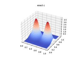
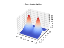
Figure 1: Left to right: exact PDE solution $u^{\dagger}$ (exact solution to the forward problem), $c^{\dagger}$ (exact solution to the inverse problem), reconstruction of $c^{\dagger}$ by (26)

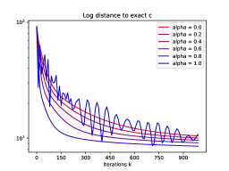
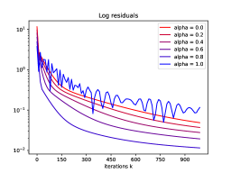
Figure 2: Results without noise: errors for $\alpha_{k}\equiv\alpha\in\{0,0.2,...,1\}$ from red to blue color. Left: distances $\|c_{k}-c^{\dagger}\|_{2}$, right: residuals $\|F(c_{k})-u^{\dagger}\|_{2}$

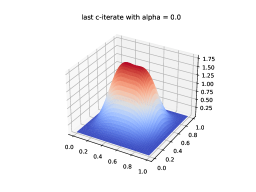
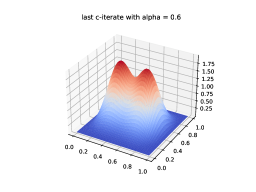
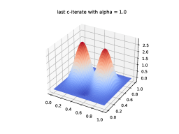
Figure 3: Results without noise, left to right: iterates $w_{10}$ for $\alpha=0$ (non-accelerated Levenberg-Marquardt method), $\alpha=0.6$ and $\alpha=1$

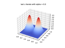
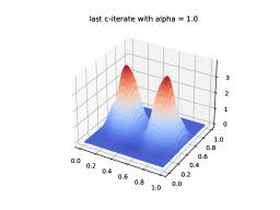
Figure 4: Results without noise, left to right: iterates $w_{500}$ for $\alpha=0$ (non-accelerated Levenberg-Marquardt method), $\alpha=0.6$ and $\alpha=1$

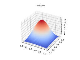
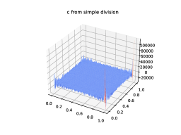
Figure 5: Left: noisy PDE solution $u^{\delta}$, right: naive approximation of $c^{\dagger}$ by (26)

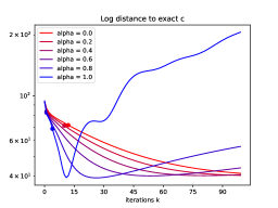
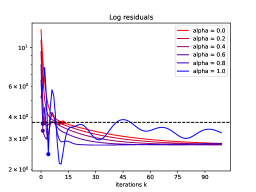
Figure 6: Results with $1\%$ of relative noise, errors for $\alpha_{k}\equiv\alpha\in\{0,0.2,...,1\}$ from red to blue color. Left: distances $\|c_{k}-c^{\dagger}\|_{2}$, right: residuals $\|F(c_{k})-u^{\dagger}\|_{2}$. Dots indicate stopping by Morozov’s discrepancy principle with $\tau=1$

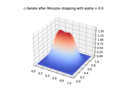
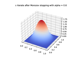
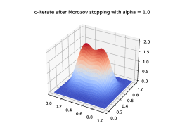
Figure 7: Results with $1\%$ of relative noise, left to right: iterates $w_{k}^{\delta}$ stopped by Morozov’s discrepancy principle with $\tau=1$ for $\alpha=0$ (non-accelerated Levenberg-Marquardt method), $\alpha=0.6$ and $\alpha=1.0$

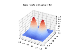
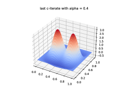
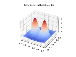
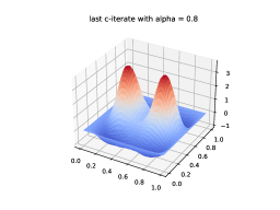
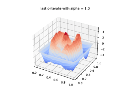
Figure 8: Results with $1\%$ of relative noise, left to right: iterates $w_{100}$ for $\alpha=k/10$ for $k=0,2,...,10$

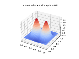
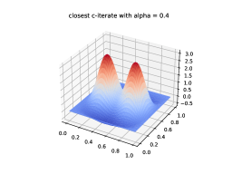
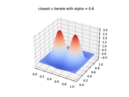
Figure 9: Results with $1\%$ of relative noise, left to right: iterates $w_{k^{*}(\alpha)}$ for $\alpha=k/10$ for $k=0,2,...,10$, where $k^{*}(\alpha)$ is the index where $w_{k}$ is closest to $c^{\dagger}$ in Euclidean norm

3.2 An inverse problem in neural network training

In this section, the problem of forecasting the concentration of CO in a gas sensor array is considered. Since we already used this model problem for numerical experiments in [25, 26], we are here brief in the description.

We utilize a dataset obtained from a gas delivery platform facility at the ChemoSignals Laboratory in the BioCircuits Institute at the University of California, San Diego (the actual data utilized here can be accessed on the UC Irvine Machine Learning Repository at https://archive.ics.uci.edu/ml/index.php, specifically under the dataset titled Gas sensor array under dynamic gas mixtures).

Formulation of the inverse problem.

This dataset comprises readings from 16 different chemical sensors exposed to varying concentrations of a mixture of Ethylene and CO in the air. The measurements were obtained through continuous acquisition of signals from the 16-sensor array over approximately 12 hours without interruption; each sensor data consists of $N=4,188,262$ scalar measurements (for a comprehensive description of the experiment, please see [11, 25]).

We address the inverse problem proposed in [25, 26] namely, to predict the reading from sensor #16, the last sensor, by leveraging the readings from the preceding sensors (see [25, Figure 3] for scatter plots of sensor $\#i$ readings against sensor #16 readings, for $i\leq 15$). As in [26], we employ a neural network (NN) in this context, which takes the readings from the first sensors as input and produces a scalar value as output, predicting the reading of the last sensor. Following [26], the structure of the NN used in our experiments reads:

— Input: $z\in\mathbb{R}^{14}$, readings of the first 14 sensors;

— Output: $NN(z;W,b)=\sigma(Wz+b)\in\mathbb{R}$.

Here $W\in R^{1\times 14}$ is a matrix of weights, $b\in R$ is a scalar bias, and $\sigma:\mathbb{R}\to\mathbb{R}$ is the activation function defined by

$$\sigma(t)=\left\{\begin{array}[]{cl}c+a(t-c)&,\ t\geq c\\ t&,\ -c<t<c\\ -c+a(t+c)&,\ t\leq-c\end{array}\right.,$$ (28)

where $0<a<1$ and $c>0$. This is a variation of the saturated linear activation function [7] (the constants $a$ and $c$ should be chosen s.t. the range of $\sigma$ contains all possible readings of sensor #16).

This is a shallow NN with only one layer (the output layer); the dimention of the corresponding parameter space is 15, the dimention of $(W,b)$. For linear $\sigma$, this NN approach simplifies to the multiple linear regression approach considered in [25]. The inverse problem under consideration is a NN training problem, i.e. one aims to find an approximate solution to the nonlinear system

$F_{i}(W,b)=y_{i}^{\delta}\,,\ \ i=0,\dots,N_{t}-1$,

where $F_{i}(W,b):=NN(z_{i};W,b)=\sigma(Wz_{i}+b)$. Here $N_{t}<N$ is the size of the training set and $z_{i}\in\mathbb{R}^{14}$ contains the readings of sensors $(\#1,\#3,\#4,\dots,\#15)$, for $i=0,\dots,N_{t}-1$. To suit our objectives, it is advantageous to express the preceding system in the form

$$\mathbf{F}(W,b)\ =\mathbf{y}^{\delta}\,,$$ (29)

where $\mathbf{F}(W,b):=\big{[}F_{i}(W,b)\big{]}_{i=0}^{N_{t}-1}$ and $\mathbf{y}^{\delta}=\big{[}y_{i}^{\delta}\big{]}_{i=0}^{N_{t}-1}$.

Remark 3.1 (On the choice of the activation function).

The real function $\sigma(t)$ in (28) is not differentiable at $t=-c$ and $t=c$. Consequently, the theoretical findings discussed in Section 2 cannot be applied to the inverse problem in (29) (indeed, the operator $\mathbf{F}$ does not satisfy (A1), (A2)). However, one observes that:

Defining $s(t):=\partial_{+}\sigma(t)$, the right derivative of $\sigma$ at $t\in\mathbb{R}$, a direct calculation shows that

$$\|\sigma(t^{\prime})-\sigma(t)-s(t)(t^{\prime}-t)\|\ \leq\ \widetilde{\eta}\|\sigma(t^{\prime})-\sigma(t)\|\ \ {\it for\ all}\ t,\,t^{\prime}\in\mathbb{R}$$ (30)

with $\widetilde{\eta}=(1-a)a^{-1}$. Therefore, for each $0\leq i<N_{t}$ the operator $F_{i}:(W,b)\mapsto\sigma(Wz_{i}+b)$, with $\sigma$ as in (28), satisfies (A2) in $\mathbb{R}^{14}\times\mathbb{R}$ with $F_{i}^{\prime}(W,b)$ replaced by $\widetilde{F}^{\prime}_{i}(W,b):\mathbb{R}^{14}\times\mathbb{R}\ni(W_{h},b_{h})\mapsto s(Wz_{i}+b)(W_{h}z_{i}+b_{h})\in\mathbb{R}$; the corresponding constant in (A2) reads $\eta_{i}=(1-a)a^{-1}\max\{\|z_{i}\|,1\}$. An immediate consequence of these facts is that $\mathbf{F}:(W,b)\mapsto\big{[}F_{i}(W,b)\big{]}_{i=0}^{N_{t}-1}$ in (29) satisfies (A2) in $\mathbb{R}^{14}\times\mathbb{R}$, with $F_{i}^{\prime}$ replaced by $\widetilde{F}^{\prime}$, for $\eta=\max_{i}\{\eta_{i}\}$.

It is well known that convergence proofs of nonlinear Landweber and LM methods can be derived under assumption (A2) where $F^{\prime}$ does not necessarily have to be the derivative of $F$ (see [15]); it only needs to be a linear operator that is uniformly bounded in a neighborhood of the initial guess $x_{0}$. We conjecture that the results obtained in Section 2 can be extended to the framework described above. This is part of our ongoing work.

For a given pair of parameters $(W,b)$, the performance $\mathcal{P}$ of the corresponding neural network $N\!N(\cdot;W,b)$ is defined by

$$\mathcal{P}(N\!N(\cdot;W,b))\ :=\ 1-\frac{1}{N_{T}}\textstyle\sum\limits_{i=N_{t}}^{N_{t}+N_{T}-1}\displaystyle\frac{\|N\!N(z_{i};W,b)-y_{i}^{\delta}\|}{\|y_{i}^{\delta}\|}\,,$$ (31)

were $N_{T}\in\mathbb{N}$ is the size of the test set. The sum in the above definition gives the average misfit betwen the predicted value $N\!N(z_{i};W,b)$ and $y_{i}^{\delta}$, evaluated over the test set $\{z_{i},\ N_{t}\leq i<N_{t}+N_{T}-1\}$. Notice that $0\leq\mathcal{P}(N\!N(\cdot;W,b))\leq 1$ for all $(W,b)$, while $\mathcal{P}(N\!N(\cdot;W,b))=1$ is the best possible performance.

Remark 3.2 (The training set and test set).

The ’training set’ and ’test set’ are comprised of samples with sizes of $N_{t}$ and $N_{T}$ respectively. In our numerical experiments we use $N_{t}=4,000,000$ and $N_{T}=100,000$ (notice that $Nt+N_{T}<N$).

Numerical implementations.

In what follows the inLM method is implemented for solving the NN training problem (29). In view of Remark 3.1 we choose $a=\frac{2}{3}$ and $c=8$ in (28). Consequently, we generate an activation function $\bar{\sigma}$ of the form (28), satisfying (30) for $\eta=0.5$.

The sensor readings $(z_{i},y_{i}^{\delta})\in\mathbb{R}^{14}\times\mathbb{R}$ on the training set are scaled by the factor $\max_{i\leq N_{t}}\|z_{i}\|$. An analogous procedure is performed on the test set. Consequently, after scaling, it holds $\|z_{i}\|\leq 1$, for $i=0,\dots,N_{t}+N_{T}$. From Remark 3.1 it follows that, for $\bar{\sigma}$ as above, all operators $F_{i}(W,b)$ satisfy (A2) (with $F^{\prime}_{i}$ replaced by $\widetilde{F}^{\prime}_{i}$) for the same constant $\eta=0.5$; the same holds for the operator $\mathbf{F}$ in (29).

In our experiments the initial guess $(W_{0},b_{0})$ is a random vector with coordinate values ranging in $(-1,1)$. We approximate the linear solve in step [2.1] of Algorithm 2 by three steps of the conjugate gradient method with zero initial value. Three different runs of the inLM method are presented, each one for a different choice of (constant) inertial parameter $\alpha_{k}$, namely $\{0.05,0,10,0.20\}$.

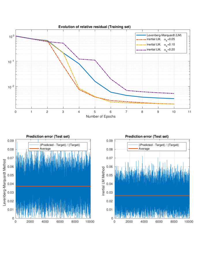
Figure 10: Neural Network training problem. (TOP) Evolution of relative residual for different methods; (BOTTOM) Prediction error of the trained NN for the test-set: LM method (left) and inLM method (right).

For comparison purposes the classical LM method ($\alpha_{k}=0$) was also implemented. Since the noise level $\delta$ is not known, all methods are computed for ten steps; after the tenth step the residual evolution stagnates for all methods. The obtained results are summarized in Figure 10:

• (TOP) Evolution of relative residual  $\sum_{i=0}^{N_{t}-1}\frac{\|N\!N(z_{i};W_{k},b_{k})-y_{i}^{\delta}\|}{\|N\!N(z_{i};W_{0},b_{0})-y_{i}^{\delta}\|}$ on the training set – all methods.

• (BOTTOM-RIGHT) inLM method: relative prediction error $\|N\!N(z_{i};W_{k^{*}},b_{k^{*}})-y_{i}^{\delta}\|/\|y_{i}^{\delta}\|$ is plotted for the test set $\{z_{i},\ N_{t}\leq i<N_{t}+N_{T}-1\}$ (BLUE); the average value (RED) is $0.026$. The performance of the trained Neural Network amounts to $\mathbf{97}$%.

• (BOTTOM-LEFT): For comparison, the prediction accuracy of the NN trained by the LM method is plotted for the same test set (BLUE), the average value is $0.037$ (RED). The performance of the trained Neural Network amounts to $\mathbf{96}$%.

Here are a few observations from our numerical experiments:

• For constant choices of $\alpha_{k}$, small values yield the best results (in our experiments $\alpha_{k}=0.05$ and $0.10$). For even smaller constant values, such as $\alpha_{k}=0.01$, the performance of the inLM method becomes very similar to that of the LM method (which corresponds to $\alpha_{k}=0$).

• For larger constant values of $\alpha_{k}$, e.g. $\alpha_{k}=0.20$, the inLM method becomes unstable and its performance deteriorates compared to that of the LM method.

• The Neural Network trained using the inLM method outperforms the one trained with the LM method. Additionally, the inLM method converges faster. The residual decay for the inLM method stagnates after 6 steps, whereas it takes 10 steps for the LM method (see Figure 10).

4 Final remarks and conclusions

In this manuscript we propose and analyze an implicit inertial type iteration, namely the inertial Levenberg Marquardt (inLM) method, as an alternative for obtaining stable approximate solutions to nonlinear ill-posed operator equations. This new method can be considered as an extension of the classical Levenberg Marquardt (LM) method (indeed, if the inertial parameters $\alpha_{k}$ are set to zero the inLM reduces to the LM method).

The main results discussed in this notes are: boundedness of the sequences $(x_{k})$ and $(w_{k})$ generated by the inLM method (Propositions 2.6 and 2.7), strong convergence for exact data (Theorem 2.9), stability and semi-convergence for noisy data (Theorems 2.14 and 2.15 respectively). We also provide a bound for the stopping index in the noisy data case (Proposition 2.13).

In Section 3 two distinct ill-posed problems are used to investigate the numerical efficiency of the proposed inLM method: A parameter identification problem in an elliptic PDE and an inverse problem in neural network training.

The preliminary results obtained in our numerical experiments indicate a better performance (faster convergence) of the inLM method when compared to the LM method. The inLM method not only converges faster than the LM method (as shown in Figures 6 and 10), but it also attains an approximate solution with a significantly smaller residual in the second inverse problem.

References

- [1] F. Alvarez and H. Attouch, An inertial proximal method for maximal monotone operators via discretization of a nonlinear oscillator with damping, Set-Valued Anal. 9 (2001), no. 1-2, 3–11.
- [2] F. Alvarez, H. Attouch, J. Bolte, and P. Redont, A second-order gradient-like dissipative dynamical system with Hessian-driven damping. Application to optimization and mechanics, J. Math. Pures Appl. (9) 81 (2002), no. 8, 747–779. MR 1930878
- [3] Hedy Attouch, Juan Peypouquet, and Patrick Redont, Fast convex optimization via inertial dynamics with Hessian driven damping, J. Differential Equations 261 (2016), no. 10, 5734–5783. MR 3548269
- [4] J. Baumeister, Stable Solution of Inverse Problems, Advanced Lectures in Mathematics, Friedr. Vieweg & Sohn, Braunschweig, 1987. MR 889048
- [5] A. Beck and M. Teboulle, A fast iterative shrinkage-thresholding algorithm for linear inverse problems, SIAM J. Imaging Sci. 2 (2009), no. 1, 183–202.
- [6] R. Boiger, A. Leitão, and B.F. Svaiter, Range-relaxed criteria for choosing the Lagrange multipliers in nonstationary iterated Tikhonov method, IMA Journal of Numerical Analysis 40 (2020), no. 1, 606–627.
- [7] P.L. Combettes and J.-C. Pesquet, Deep neural network structures solving variational inequalities, Set-Valued Var. Anal. 28 (2020), no. 3, 491–518.
- [8] A. De Cezaro, J. Baumeister, and A. Leitão, Modified iterated Tikhonov methods for solving systems of nonlinear ill-posed equations, Inverse Probl. Imaging 5 (2011), no. 1, 1–17.
- [9] H.W. Engl, On the choice of the regularization parameter for iterated Tikhonov regularization of ill-posed problems, J. Approx. Theory 49 (1987), no. 1, 55–63.
- [10] H.W. Engl, M. Hanke, and A. Neubauer, Regularization of Inverse Problems, Kluwer Academic Publishers, Dordrecht, 1996.
- [11] J. Fonollosa, S. Sheik, R. Huerta, and S. Marco, Reservoir computing compensates slow response of chemosensor arrays exposed to fast varying gas concentrations in continuous monitoring, Sensors and Actuators B: Chemical 215 (2015), 618–629.
- [12] C. W. Groetsch and O. Scherzer, Non-stationary iterated Tikhonov-Morozov method and third-order differential equations for the evaluation of unbounded operators, Math. Methods Appl. Sci. 23 (2000), no. 15, 1287–1300.
- [13] M. Hanke and C. W. Groetsch, Nonstationary Iterated Tikhonov Regularization, J. Optim. Theory Appl. 98 (1998), no. 1, 37–53.
- [14] M. Hanke, A. Neubauer, and O. Scherzer, A convergence analysis of Landweber iteration for nonlinear ill-posed problems, Numer. Math. 72 (1995), 21–37.
- [15] B. Kaltenbacher, A. Neubauer, and O. Scherzer, Iterative Regularization Methods for Nonlinear Ill-Posed Problems, Radon Series on Computational and Applied Mathematics, vol. 6, Walter de Gruyter GmbH & Co. KG, Berlin, 2008.
- [16] S. Kindermann and A. Neubauer, On the convergence of the quasioptimality criterion for (iterated) Tikhonov regularization, Inverse Probl. Imaging 2 (2008), no. 2, 291–299.
- [17] A. Kirsch, An Introduction to the Mathematical Theory of Inverse Problems, Applied Mathematical Sciences, vol. 120, Springer-Verlag, New York, 1996.
- [18] Dirk A. Lorenz and Thomas Pock, An inertial forward-backward algorithm for monotone inclusions, J. Math. Imaging Vision 51 (2015), no. 2, 311–325. MR 3314536
- [19] B. Martinet, Régularisation d’inéquations variationnelles par approximations successives, Rev. Française Informat. Recherche Opérationnelle 4 (1970), no. Sér. R-3, 154–158.
- [20] A. Moudafi and M. Oliny, Convergence of a splitting inertial proximal method for monotone operators, J. Comput. Appl. Math. 155 (2003), no. 2, 447–454.
- [21] Y.E. Nesterov, A method for solving the convex programming problem with convergence rate , Dokl. Akad. Nauk SSSR 269 (1983), no. 3, 543–547.
- [22] Yurii Nesterov, Introductory lectures on convex optimization, Applied Optimization, vol. 87, Kluwer Academic Publishers, Boston, MA, 2004, A basic course. MR 2142598
- [23] B. T. Poljak, Some methods of speeding up the convergence of iterative methods, Ž. Vyčisl. Mat i Mat. Fiz. 4 (1964), 791–803. MR 169403
- [24] J. Rabelo, A. Leitão, and A.L. Madureira, On inertial iterated-tikhonov methods for solving linear ill-posed problems, Inverse Problems 40 (2024), no. 3, 035002.
- [25] J.C. Rabelo, Y. Saporito, and A. Leitão, On stochastic Kaczmarz type methods for solving large scale systems of ill-posed equations, Inverse Problems 38 (2022), no. 2, 025003.
- [26] , On projective stochastic-gradient type methods for solving large scale systems of nonlinear ill-posed equations: Applications to machine learning, Inverse Problems (2024), submitted.
- [27] R.T. Rockafellar, Monotone operators and the proximal point algorithm, SIAM J. Control Optim. 14 (1976), no. 5, 877–898.
- [28] O. Scherzer, Convergence rates of iterated Tikhonov regularized solutions of nonlinear ill-posed problems, Numer. Math. 66 (1993), no. 2, 259–279.
- [29] Weijie Su, Stephen Boyd, and Emmanuel J. Candès, A differential equation for modeling Nesterov’s accelerated gradient method: theory and insights, J. Mach. Learn. Res. 17 (2016), Paper No. 153, 43. MR 3555044