Learning Discrete Latent Variable Structures with Tensor Rank Conditions
Abstract
Unobserved discrete data are ubiquitous in many scientific disciplines, and how to learn the causal structure of these latent variables is crucial for uncovering data patterns. Most studies focus on the linear latent variable model or impose strict constraints on latent structures, which fail to address cases in discrete data involving non-linear relationships or complex latent structures. To achieve this, we explore a tensor rank condition on contingency tables for an observed variable set , showing that the rank is determined by the minimum support of a specific conditional set (not necessary in ) that d-separates all variables in . By this, one can locate the latent variable through probing the rank on different observed variables set, and further identify the latent causal structure under some structure assumptions. We present the corresponding identification algorithm and conduct simulated experiments to verify the effectiveness of our method. In general, our results elegantly extend the identification boundary for causal discovery with discrete latent variables and expand the application scope of causal discovery with latent variables.
1 Introduction
Social scientists, psychologists, and researchers from various disciplines are often interested in understanding causal relationships between the latent variables that cannot be measured directly, such as depression, coping, and stress [1]. A common approach to grasp these latent concepts is to construct a measurement model. For instance, experts design a set of measurable items or survey questions that serve as indicators of the latent variable and then use them to infer causal relationships among latent variables [2, 3, 4].
Numerous approaches exist for addressing structure learning among latent variables. In particular, if the data generation process is assumed to be a linear relationship, known as linear latent variable models, several approaches have been developed. These include the second-order statistic-based approaches [1, 5, 6, 7], high-order moments-based ones [8, 9, 10, 11], matrix decomposition-based methods [12, 13, 14], and copula model-based approaches [4]. Moreover, the hierarchical latent variable structure has been well-studied within the linear setting [15, 16, 17, 18]. However, the linear assumption is rather restrictive and the discrete data in the real world could be more frequently encountered (e.g., responses from psychological and educational assessments or social science surveys [19, 20]), which does not satisfy the linear assumption.
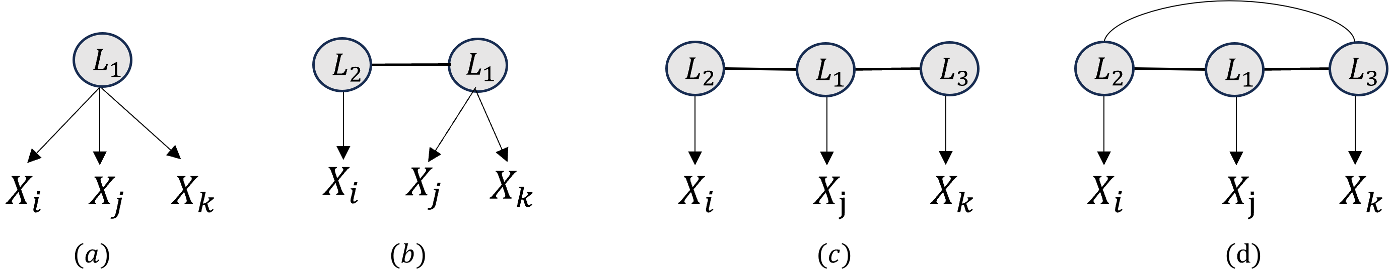
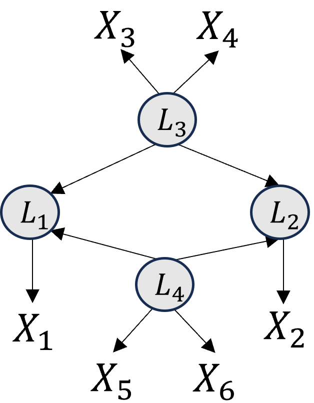
When the data generation process is discrete, however, due to the challenging nonlinear transition relationship in discrete data, few identifiability results exist and are mostly only applicable in strict cases. In particular, under some prespecified structure, the identifiability of parameters is established, such as in the hidden Markov model(HMM) [21] model, topic models [13], and multiview mixtures model [14]. By further specifying the latent variable structure as a tree, [22, 23] show that the structural model is identifiable. Recently, [24, 25] further considered the identifiability of pyramid structure under the condition that each latent variable has at least three observed children. However, challenges persist in extending identifiability to more general structures among discrete latent variables. Existing approaches, unfortunately, cannot identify the causal structure of latent variables as shown in Fig. 2(a).
In this paper, we seek to find out a general identification criteria to identify the discrete latent structure in the case where the structure is not limited to a tree-structured graph or pyramid structure. To achieve this, we explore a tensor rank condition on the contingency tables for an observed variable set , to probe the latent causal structure from observed data. Interestingly, as shown in Fig. 1, we found that the rank of the contingency tables of the joint distribution is deeply connected to the support of a variable (not necessary among ) that d-separate and . By this observation, we first develop a general tensor rank condition for the discrete causal model and show that such a rank is determined by the minimal support of a specific conditional set (not necessary in ) that d-separates all variables in . Such findings intrigue the possibility to identify the discrete latent variables structure. We further propose a discrete latent structure model that accommodates more general latent structures and shows that the discrete latent variable structure can be identified locally and iteratively through tensor rank conditions. Subsequently, we present an identification algorithm to complete the identifiability of discrete latent structure models, including the measurement model and the structure model. We theoretically show that under proper causal assumptions, such as faithfulness and the Markov assumption, the measurement model is fully identifiable and the structure model can be identified up to a Markov equivalence class.
The contributions of this work are three-fold. (1) We first establish a connection between the tensor rank condition and the graphical patterns in a general discrete causal model, including specific d-separation relations. (2) We then exploit the tensor rank condition to learn the discrete latent variable model, allowing flexible relations between latent variables. (3) We present a structure learning algorithm using tensor rank conditions and demonstrate the effectiveness of the proposed algorithm through simulation studies.
2 Discrete Latent Structure Model
For an integer , denote . Consider a discrete statistic model with latent variable set and discrete observed variable set with (), in which any marginal probabilities are non-zero. We say a discrete statistic model is a discrete causal model if and only if can be represented by a directed acyclic graph (DAG), denoted by . We use to denote the set of possible values of the random variable . Our work is in the framework of causal graphical models. Concepts used here without explicit definition, such as d-separation, which can refer to standard literature [26].
In this paper, we focus on learning causal structure among latent variables in one class of discrete causal models. The model is defined as follows.
Definition 2.1 (Discrete Latent Structure Model).
A discrete causal model is the Discrete Latent Structure Model (Discrete LSM) if it further satisfies the following three assumptions:
-
1)
[Purity Assumption] there is no direct edges between the observed variables;
-
2)
[Three-Pure Child Variable Assumption] each latent variable has at least three pure variables as children;
-
3)
[Sufficient Observation Assumption] The dimension of observed variables support is larger than the dimension of any latent variables support.
These structural constraints inherent in the discrete LSM are also widely used in linear latent variable models, e.g., [1, 5, 10, 8]. In the binary latent variable case, recently, a similar definition is also employed in [25, 24]. The key difference is that there are no constraints on the latent structure in our work. An example of a discrete LSM model is shown in Fig. 2(a), where represent discrete latent variables, and are discrete observed (measured) variables.
In general, the discrete LSM model can be divided into two sub-models [26], i.e., the measurement model and the structure model, e.g., red edge and blue edge in Fig. 2 (a). By this, one can first identify the measurement model to determine the latent variables and then use the measured variable to infer the causal structure of latent variables. As shown in Fig. 2 (b), we will respectively discuss the identification of two sub-models and show that the measurement model is fully identifiable and the structure model is identified up to a Markov equivalence class. The symbols used in our work is summarised in Table 1.
To ensure the identification of causal structure and the asymptotic correctness of identification algorithms, some common causal assumptions are required.
Assumption 2.2 (Causal Markov Assumption).
Let be a causal graph with vertex set and be probability distribution over the vertices in generated by . We say and satisfy the Causal Markov Assumption if and only if for every , .
Assumption 2.3 (Faithfulness Assumption).
Let be a causal graph with vertex set and be probability distribution over the vertices in generated by . We say satisfies the Faithfulness Assumption if and only if (i). every conditional independence relation true in is entailed by the Causal Markov Assumption applied to , and (ii). for any joint distribution , there does not exist with such that .
Assumption 2.4 (Full Rank Assumption).
For any conditional probability , the corresponding contingency table is full rank, i.e., each column of is linearly independent with the other column vectors in the parameter space.
The Causal Markov Assumption and Faithfulness Assumption are widely used in the constraint-based causal discovery methods, e.g., PC algorithm and FCI algorithm [26, 27]. One can see that we further constraint the parameter space of joint distribution cannot be reduced to a low-dimension space, for maintaining the diversity of parameter space. This is also the reason for the full rank assumption, which has also been used in related studies [24].
Our goal: The target of our work is to answer the identification of the discrete latent structure model, including the measurement model and the structure model.
: The set of variables : The set of observed variables : The set of latent variables : Conditional independence : Dimension of : the tensor form of : the joint distribution of : The rank of tensor : The parent set of : The descendant set of : The diagonal matrix of : The outer product of two vectors
3 Tensor Rank Condition with Graphical Criteria
To address the identification problem in the discrete LSM, this section introduces the building block–the tensor rank condition of the discrete causal model. Then, we establish the connection between tensor rank and d-separation relations under a general discrete causal model.
Before formalizing the tensor rank condition, we first give the explicit definition of tensor rank.
Definition 3.1 (Rank-one Tensor).
An n-way tensor is a rank-one tensor if it can be written as the outer product of vectors, i.e.,
where are vectors that each represent a dimension of the tensor, represents the outer product.
Definition 3.2 (Tensor Rank [28]).
For an n-way tensor , the rank of a tensor is defined as the smallest number of rank-one tensors that sum to exactly represent . Formally, the rank of tensor , denoted , is the smallest integer such that:
where each is a vector in the corresponding vector space associated with the -th mode of .
In other words, the tensor rank denotes the minimal number of rank-one decompositions. In the discrete causal model, the joint distribution can be represented as a tensor, e.g., the joint distribution of two random variables is a two-way contingency tensor. Interestingly, by carefully analyzing the rank-one decomposition of the joint distribution, we find that the tensor rank essentially reveals structural information within the causal graph. The result is shown below.
Theorem 3.3 (Graphical implication of tensor rank condition).
In the discrete causal model, suppose Assumption 2.2 Assumption 2.4 holds. Consider an observed variable set ( and ) and the corresponding n-way probability tensor that is the tabular representation of the joint probability mass function , then () if and only if (i) there exists a variable set with that d-separates any pair of variables in , and (ii) does no exist conditional set that satisfies .
We further provide an example to illustrate Theorem 3.3, and a more comprehensive case is provided in Appendix B.
Example 3.4 (Illustrating for the graphical criteria).
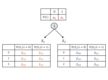
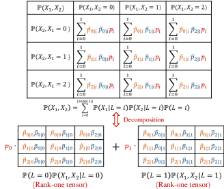
Consider a single latent variable structure as shown in Fig. 1 (a) where is a latent variable with and are observed variables with . For convenience, we denote , , and . For the joint distribution of , it can be represented by the product of conditional probability, as shown in Fig. 1(b). By applying the tensor decomposition, one can see that can be decomposed as the sum of two rank-one tensors: and , i.e., the rank of the tensor is two that related to the dimension of the latent support. The reason that is a rank-one tensor is that d-separates and , i.e., . This illustrates a connection between tensor rank and the d-separation relations.
Intuitively, the graphical criteria theorem suggests that, in the discrete causal model, the tensor rank condition implies the minimal conditional probability decomposition within the probability parameter space, which hopefully induces the structural identifiability of the discrete LSM model.
4 Structure Learning of Discrete Latent Structure Model
In this section, we address the identification problem of the discrete LSM model using a carefully designed algorithm that leverages the tensor rank condition. Specifically, we first show that latent variables can be identified by finding causal clusters among observed variables (Sec. 4.1). Then, we use these causal clusters to conduct conditional independence tests among latent variables based on the tensor rank condition, identifying the structure model (Sec. 4.2). Finally, we discuss the practical implementation of testing tensor rank (Sec. 4.3). For simplicity, we focus on the case where all latent variables have the same number of categories, with extensions provided in Appendix E.
4.1 Identification of the measurement model
To answer the identification of the measurement model, one common strategy is to find the causal cluster that shares the common latent parent, which has been well-studied within the linear model, such as [1, 10, 8]. We follow this strategy and show that, in the discrete LSM, the causal cluster can be found by testing the tensor rank conditions iteratively. The definition of a causal cluster is as follows.
Definition 4.1 (Causal cluster).
In the discrete LSM model, the observed is a causal cluster, termed , if and only if all variables in share the common latent parent.
It is not hard to see that, the measurement model can be identified if all causal cluster is found. In order to find these causal clusters by making use of the tensor rank condition, the key issue is to determine the support of latent variables in advance. This issue can be addressed by identifying the rank of the two-way tensor formed by the joint distribution of two observed variables
Proposition 4.2 (Identification of support of latent variables).
This result holds because any pair of variables in the discrete LSM model is d-separated by any one of their latent parent variables, and all latent variables have the same support. Next, we formalize the property of clusters and give the criterion for finding clusters.
Proposition 4.3 (Identification of causal cluster).
In the discrete LSM mode, suppose Assumption 2.2 Assumption 2.4 holds. Let be the dimension of latent support, for three disjoint observed variables ,
-
•
: if the rank of tensor is not equal to , i.e., , then , and belong to the different latent parent.
-
•
: for any , , the rank of tensor is , i.e., , then share the same latent parent.
Example 4.4 (Finding causal clusters).
Let’s take Fig. 2(a) as an example. One can find that for , where , the rank of tensor is . Thus, is identified as a causal cluster.
Next, we consider the practical issues involved in determining the number of latent variables by causal clusters. That is, there are some causal clusters that should be merged because they share one latent parent. We find that the overlapping clusters can be directly merged into one cluster. This is because the overlapping clusters have the same latent variable as the parent under the discrete LSM model. The validity of the merge step is guaranteed by Proposition 4.5.
Proposition 4.5 (Merging Rule).
In the discrete LSM model, for two causal clusters and , if , then and share the same latent parent.
Based on the above results, one can iteratively identify causal clusters and apply the merger rule to detect all latent variables. The identification procedure is summarized in Algorithm 1.
Input: Data from a set of measured variables , and the dimension of latent support
Output: Causal cluster
4.2 Identification of the structure model
Once the measurement model is identified, the observed children can serve as proxies for the latent variables, enabling the identification of the causal structure among them. Here, we employ constraint-based framework to learn the causal structure of latent variables.
Constraint-based structure learning algorithms find the Markov equivalence class over a set of variables by making decisions about independence and conditional independence among them. Given a pure and accurate measurement model with at least two measures per latent variable, we can test for independence and conditional independence (CI) among the latent variables. Specifically, to test statistical independence between discrete variables, one can examine whether the rank of their joint distribution contingency table is one [29]. For testing conditional independence (CI) relations among latent variables, further leveraging the algebraic properties of the tensor rank condition is required (see Theorem 4.7).
Theorem 4.7 (d-separation among latent varaible).
Intuitively, based on the graphical criteria of tensor rank condition, is a minimal conditional set in the causal graph that d-separates and and hence the rank of tensor is the dimension of support of , if and also be d-separated by . An illustrative example is given below.
Example 4.8 (CI test among latent variables).
Consider the structure in Fig. 2(a). Suppose . By selecting and to be two disjoint child set of respectively, let , one can see that the rank of tensor is four (due to is minimal conditional set that d-separates any pair variable in ), which imply that .
Based on Theorem 4.7, we introduce the PC-TENSOR-RANK algorithm. This method accepts a measurement model learned by the previous procedure, and outputs the Markov equivalence class of the structural model associated with the latent variables within the measurement model, in accordance with the PC algorithm. The implementation is summarised as Algorithm 2. Consequently, we establish the identification of the structure model as shown in Theorem 4.9.
Input: Data set and causal cluster
Output: A partial DAG .
4.3 Practical Test for Tensor Rank
In our theoretical results, the key issue is to test the rank of a tensor, which involves estimating the dimension of latent support and the rank of a tensor. Here, we aim to explore methods to (i) estimate the rank of the contingency matrix for determining the dimension of latent support, and (ii) apply the goodness-of-fit test to assess the tensor rank.
Estimate the rank of contingency matrix.
We start with the estimation of the dimension of latent variables support based on Prop. 4.2. There are many practical approaches used to estimate the rank of a general matrix , such as [31]. In our implementation, we use the characteristic root statistic, abbreviated as CR statistic [32], to test the rank of the probability contingency matrix of two observed variables. Specifically, Let be an asymptotically normal estimator of , then the CR statistic is the sum of smallest singular values of , multiplied by the sample size. Under the null hypothesis, the above statistic converges in distribution to a weighted (given by the eigenvalues) sum of independent random variables [32].
Goodness-of-fit test for tensor rank.
Once the dimension of the support of latent variables is identified, in the structure learning procedure, we perform the following hypotheses test: : v.s. : . To achieve this, we first apply the CP decomposition technology to the target tensor as a sum of rank-one tensors given specified , then we evaluate how well the reconstructed tensor from this decomposition approximates the original tensor to conduct the hypotheses test.
To perform the rank-decomposition with specified on the probability contingency tensor, one can use the non-negative CP decomposition to decompose the tensor into the sum of rank-one tensor [33]. Given the decomposition, one can obtain a reconstructed tensor, denoted by , from the outer product of decomposed vectors.
With the reconstructed tensor, we constructed square-chi goodness of fit test [34] for testing . Such a test is frequently used to summarize the discrepancy between observed values and the expected values, which measure the sum of differences between observed and expected outcome frequencies. Let be the vectorization of tensor , suppose be the asymptotic normality estimator of , we have the chi-square statistic as , which follows the distribution with freedom degrees .
5 Simulation Studies
In this section, we conducted simulation studies to assess the correctness of the proposed methods in causal structure learning tasks. The baseline approaches include Building Pure Cluster (BPC) [1], Latent Tree Model (LTM) [35], and Bayesian Pyramid Model (BayPy) [25].
In the following simulation studies, we consider the different combinations of various types of structure models(SM) and measurement models(MM). Specifically, for the structure model, we consider the following five typical cases: [SM1]: ; [SM2]: ; [SM3]: the structure of latent variables is shown in Fig. 2(a); [Collider]: ; [Star]: . For the measurement model, we consider the following two cases: [MM1]: each latent variable has three pure observed variables, i.e., ; [MM2]: each latent variable has four pure observed variables, i.e., .
In all cases, the data generation process follows the discrete LSM model: (i) we generate the probability contingency table of latent variables in advance, according to different latent structures (e.g., SM1), then (ii) we generate the conditional contingency table of observed variables (condition on their latent parent), and finally (iii) we sample the observed data according to the probability contingency table, where the dimension of latent support is set to 3 and the dimension of all observed variables support is set to 4, sample size ranged from .
For each simulation study, we randomly generate the dataset and apply the proposed algorithm and baselines to these data. We use the following scores for evaluating the performance of causal clusters from each algorithm: latent omission, latent commission, and mismeasurement. Moreover, to assess the ability of these algorithms to correctly discover the causal structure among latent variables, we use the metric like edge omission (EO), edge commission (EC), and orientation omission (OO). These metrics can be referred to [1], in which the tasks are aligned with our work. Each experiment was repeated ten times with randomly generated data, and the results were averaged.
| Latent omission | Latent commission | Mismeasurements | |||||||||||
|---|---|---|---|---|---|---|---|---|---|---|---|---|---|
| Algorithm | Our | BayPy | LTM | BPC | Our | BayPy | LTM | BPC | Our | BayPy | LTM | BPC | |
| 5k | 0.15(3) | 0.10(2) | 0.15(3) | 0.96(10) | 0.00(0) | 0.10(2) | 0.00(0) | 0.00(0) | 0.05(1) | 0.00(0) | 0.00(0) | 0.00(0) | |
| 10k | 0.05(1) | 0.05(1) | 0.10(2) | 0.90(10) | 0.00(0) | 0.05(1) | 0.00(0) | 0.00(0) | 0.00(0) | 0.00(0) | 0.00(0) | 0.00(0) | |
| 50k | 0.00(0) | 0.00(0) | 0.00(0) | 0.90(10) | 0.00(0) | 0.00(0) | 0.00(0) | 0.00(0) | 0.00(0) | 0.00(0) | 0.00(0) | 0.00(0) | |
| 5k | 0.23(5) | 0.19(6) | 0.26(6) | 0.90(10) | 0.00(0) | 0.19(6) | 0.03(1) | 0.00(0) | 0.05(2) | 0.19(6) | 0.23(6) | 0.00(0) | |
| 10k | 0.13(4) | 0.13(4) | 0.13(4) | 0.86(10) | 0.00(0) | 0.03(4) | 0.00(0) | 0.00(0) | 0.00(0) | 0.13(4) | 0.13(4) | 0.00(0) | |
| 50k | 0.06(2) | 0.10(3) | 0.10(3) | 0.86(10) | 0.00(0) | 0.13(4) | 0.00(0) | 0.00(0) | 0.00(0) | 0.13(4) | 0.10(3) | 0.00(0) | |
| 5k | 0.12(2) | 0.19(6) | 0.21(5) | 0.90(10) | 0.00(0) | 0.19(6) | 0.00(0) | 0.00(0) | 0.03(1) | 0.16(6) | 0.21(5) | 0.00(0) | |
| 10k | 0.03(1) | 0.13(4) | 0.10(3) | 0.86(10) | 0.00(0) | 0.13(4) | 0.00(0) | 0.00(0) | 0.00(0) | 0.11(4) | 0.10(3) | 0.00(0) | |
| 50k | 0.00(0) | 0.07(2) | 0.07(2) | 0.83(10) | 0.00(0) | 0.07(2) | 0.00(0) | 0.00(0) | 0.00(0) | 0.07(2) | 0.06(2) | 0.00(0) | |
| 5k | 0.25(6) | 0.30(6) | 0.55(10) | 0.86(10) | 0.00(0) | 0.30(6) | 0.00(0) | 0.00(0) | 0.12(5) | 0.20(6) | 0.55(10) | 0.00(0) | |
| 10k | 0.17(5) | 0.25(5) | 0.50(10) | 0.83(10) | 0.00(0) | 0.25(5) | 0.00(0) | 0.00(0) | 0.05(3) | 0.16(5) | 0.50(10) | 0.00(0) | |
| 50k | 0.08(3) | 0.20(4) | 0.50(10) | 0.83(10) | 0.00(0) | 0.20(4) | 0.00(0) | 0.00(0) | 0.03(2) | 0.13(4) | 0.50(10) | 0.00(0) | |
| Edge omission | Edge commission | Orientation omission | |||||||||||
|---|---|---|---|---|---|---|---|---|---|---|---|---|---|
| Algorithm | Our | BayPy | LTM | BPC | Our | BayPy | LTM | BPC | Our | BayPy | LTM | BPC | |
| 5k | 0.00(0) | 1.00(10) | 0.26(8) | 1.00(10) | 0.10(1) | 0.00(0) | 0.00(0) | 0.00(0) | 0.10(1) | 1.00(10) | – | 1.00(0) | |
| Collider+ | 10k | 0.00(0) | 1.00(10) | 0.23(6) | 1.00(10) | 0.00(0) | 0.02(1) | 0.0(0) | 0.00(0) | 0.00(0) | 1.00(10) | – | 1.00(0) |
| 50k | 0.00(0) | 1.00(10) | 0.10(3) | 1.00(10) | 0.00(0) | 0.00(0) | 0.00(0) | 0.00(0) | 0.00(0) | 1.00(10) | – | 1.00(0) | |
| 5k | 0.15(3) | 1.00(10) | 0.16(6) | 1.00(10) | 0.10(1) | 0.00(0) | 0.00(0) | 0.00(0) | 0.00(0) | 0.00(0) | – | 0.00(0) | |
| 10k | 0.05(1) | 1.00(10) | 0.13(4) | 1.00(10) | 0.01(1) | 0.00(0) | 0.00(0) | 0.00(0) | 0.00(0) | 0.00(0) | – | 0.00(0) | |
| 50k | 0.00(0) | 1.00(10) | 0.10(3) | 1.00(10) | 0.00(0) | 0.00(0) | 0.00(0) | 0.00(0) | 0.00(0) | 0.00(0) | – | 0.00(0) | |
| 5k | 0.10(3) | 1.00(10) | 0.25(5) | 1.00(10) | 0.20(5) | 0.00(0) | 0.00(0) | 0.00(0) | 0.00(0) | 0.00(0) | – | 0.00(0) | |
| 10k | 0.06(2) | 1.00(10) | 0.15(3) | 1.00(10) | 0.08(3) | 0.00(0) | 0.00(0) | 0.00(0) | 0.00(0) | 0.00(0) | – | 0.00(0) | |
| 50k | 0.03(1) | 1.00(10) | 0.15(3) | 1.00(10) | 0.05(2) | 0.00(0) | 0.00(0) | 0.00(0) | 0.00(0) | 0.00(0) | – | 0.00(0) | |
| 5k | 0.22(7) | 1.00(10) | 0.50(10) | 1.00(10) | 0.40(6) | 0.00(0) | 0.02(1) | 0.00(0) | 0.20(2) | 1.00(10) | – | 1.00(10) | |
| 10k | 0.15(5) | 1.00(10) | 0.50(10) | 1.00(10) | 0.10(2) | 0.00(0) | 0.00(0) | 0.00(0) | 0.10(1) | 1.00(10) | – | 1.00(10) | |
| 50k | 0.05(2) | 1.00(10) | 0.50(10) | 1.00(10) | 0.05(1) | 0.00(0) | 0.00(0) | 0.00(0) | 0.00(0) | 1.00(10) | – | 1.00(10) | |
The results are reported in Table 2 and Table 3. Our method consistently delivers the best outcomes across most scenarios, demonstrating its capability to identify both the causal clusters and the causal structures of latent variables. In contrast, the BPC approach performs poorly, as it is specifically designed for linear models. Additionally, the LTM and BayPy algorithms show suboptimal performance in structure learning of latent variables due to their limitations to specific structural models, such as tree structures, or assumptions that latent variables are binary. More experimental results and discussions are provided in the appendix.
6 Real Data Applications
We now briefly present the results from two real datasets. The first is the political efficacy dataset, collected by [36] through a cross-national survey designed to capture information on both conventional and unconventional forms of political participation in industrial societies. This dataset includes 1719 cases obtained in a USA sample. The second dataset, referred to as the depress dataset, is detailed by [37] and comprises twelve observed variables grouped into three latent factors: self-esteem, depression, and impulsiveness, with a total of 204 samples. Our algorithm learns the correct causal structure (including the measurement model and the structure model) for both datasets by first identifying the dimension of latent support as two in the political efficacy dataset and four in the depress dataset. See the appendix for more details.
7 Discussion and Further Work
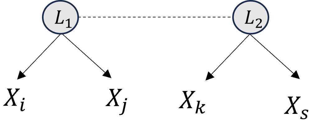
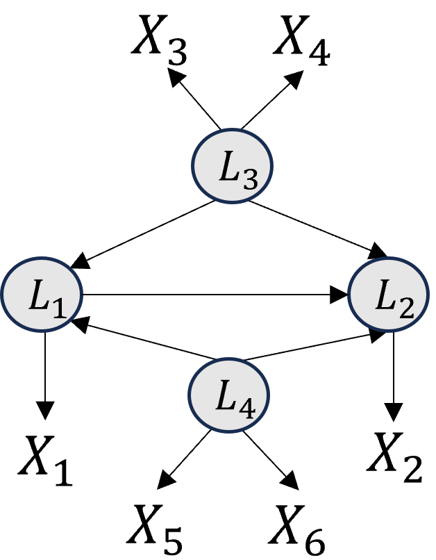
The preceding sections presented how to use tensor rank conditions to locate the latent variables and identify their causal structure in the discrete LSM model. In this section, we examine whether the impure structure (e.g., an edge between observed variables) can be detected through tensor rank conditions. For instance, consider the structure shown in Fig. 3. One can observe that for any subset where , one has . This implies and (or ) share the common latent parent. Meanwhile, we have . Moreover, we have . By the graphical criteria of tensor rank condition, one can infer that there is an edge between and , indicating the impure structure can be identified by the tensor rank condition. Developing an efficient algorithm to learn a more general discrete LSM structure that allows impure structure in a principled way is part of our future work.
8 Conclusion
We derive a nontrivial algebraic property of a particular type of discrete causal model under proper causal assumptions. We build the connection between tensor rank and the d-separation relations in the causal graph and propose the graphical criteria of tensor rank. By this, the identifiability of causal structure in discrete latent structure models is achieved based on which we proposed an identification to locate latent causal variables and identify their causal structure. We provide a practical test approach for testing the tensor rank and verifying the efficientness of the proposed algorithm via the simulated studies. The proposed theorems and the algorithms take a meaningful step in understanding the causal mechanism of discrete data. Future research along this line includes allowing casual edges between observed variables and allowing hierarchical latent structure.
References
- Silva et al. [2006] Ricardo Silva, Richard Scheine, Clark Glymour, and Peter Spirtes. Learning the structure of linear latent variable models. JMLR, 7(Feb):191–246, 2006.
- Bollen [2002] Kenneth A Bollen. Latent variables in psychology and the social sciences. Annual review of psychology, 53(1):605–634, 2002.
- Bartholomew et al. [2011] David J Bartholomew, Martin Knott, and Irini Moustaki. Latent variable models and factor analysis: A unified approach. John Wiley & Sons, 2011.
- Cui et al. [2018] Ruifei Cui, Perry Groot, Moritz Schauer, and Tom Heskes. Learning the causal structure of copula models with latent variables. In Proceedings of the Thirty-Fourth Conference on Uncertainty in Artificial Intelligence, UAI 2018, pages 188–197. AUAI Press, 2018.
- Kummerfeld and Ramsey [2016] Erich Kummerfeld and Joseph Ramsey. Causal clustering for 1-factor measurement models. In KDD, pages 1655–1664. ACM, 2016.
- Chen et al. [2024] Zhengming Chen, Jie Qiao, Feng Xie, Ruichu Cai, Zhifeng Hao, and Keli Zhang. Testing conditional independence between latent variables by independence residuals. IEEE Transactions on Neural Networks and Learning Systems, 2024.
- Sullivant et al. [2010] Seth Sullivant, Kelli Talaska, Jan Draisma, et al. Trek separation for gaussian graphical models. The Annals of Statistics, 38(3):1665–1685, 2010.
- Xie et al. [2020] Feng Xie, Ruichu Cai, Biwei Huang, Clark Glymour, Zhifeng Hao, and Kun Zhang. Generalized independent noise conditionfor estimating latent variable causal graphs. In NeurIPS, pages 14891–14902, 2020.
- Chen et al. [2022] Zhengming Chen, Feng Xie, Jie Qiao, Zhifeng Hao, Kun Zhang, and Ruichu Cai. Identification of linear latent variable model with arbitrary distribution. In Proceedings 36th AAAI Conference on Artificial Intelligence (AAAI), 2022.
- Cai et al. [2019] Ruichu Cai, Feng Xie, Clark Glymour, Zhifeng Hao, and Kun Zhang. Triad constraints for learning causal structure of latent variables. In NeurIPS, pages 12863–12872, 2019.
- Adams et al. [2021] J. Adams, N. Hansen, and K. Zhang. Identification of partially observed linear causal models: Graphical conditions for the non-gaussian and heterogeneous cases. In Advances in Neural Information Processing Systems, 2021.
- Anandkumar et al. [2013] Animashree Anandkumar, Daniel Hsu, Adel Javanmard, and Sham Kakade. Learning linear bayesian networks with latent variables. In International Conference on Machine Learning, pages 249–257, 2013.
- Anandkumar et al. [2014] Animashree Anandkumar, Rong Ge, Daniel J Hsu, Sham M Kakade, Matus Telgarsky, et al. Tensor decompositions for learning latent variable models. J. Mach. Learn. Res., 15(1):2773–2832, 2014.
- Anandkumar et al. [2015] Animashree Anandkumar, Rong Ge, and Majid Janzamin. Learning overcomplete latent variable models through tensor methods. In Conference on Learning Theory, pages 36–112. PMLR, 2015.
- Huang et al. [2022] Biwei Huang, Charles Jia Han Low, Feng Xie, Clark Glymour, and Kun Zhang. Latent hierarchical causal structure discovery with rank constraints. In Advances in Neural Information Processing Systems, 2022.
- Xie et al. [2022] Feng Xie, Biwei Huang, Zhengming Chen, Yangbo He, Zhi Geng, and Kun Zhang. Identification of linear non-gaussian latent hierarchical structure. In International Conference on Machine Learning, pages 24370–24387. PMLR, 2022.
- Chen et al. [2023] Zhengming Chen, Feng Xie, Jie Qiao, Zhifeng Hao, and Ruichu Cai. Some general identification results for linear latent hierarchical causal structure. In Proceedings of the Thirty-Second International Joint Conference on Artificial Intelligence, pages 3568–3576, 2023.
- Jin et al. [2023] Songyao Jin, Feng Xie, Guangyi Chen, Biwei Huang, Zhengming Chen, Xinshuai Dong, and Kun Zhang. Structural estimation of partially observed linear non-gaussian acyclic model: A practical approach with identifiability. In The Twelfth International Conference on Learning Representations, 2023.
- Eysenck et al. [2021] Sybil BG Eysenck, Paul T Barrett, and Donald H Saklofske. The junior eysenck personality questionnaire. Personality and Individual Differences, 169:109974, 2021.
- Skinner [2019] Chris Skinner. Analysis of categorical data for complex surveys. International Statistical Review, 87:S64–S78, 2019.
- Anandkumar et al. [2012] Animashree Anandkumar, Daniel Hsu, and Sham M Kakade. A method of moments for mixture models and hidden markov models. In Conference on learning theory, pages 33–1. JMLR Workshop and Conference Proceedings, 2012.
- Wang et al. [2017] Xiaofei Wang, Jianhua Guo, Lizhu Hao, and Nevin L Zhang. Spectral methods for learning discrete latent tree models. Statistics and Its Interface, 10(4):677–698, 2017.
- Song et al. [2013] Le Song, Mariya Ishteva, Ankur Parikh, Eric Xing, and Haesun Park. Hierarchical tensor decomposition of latent tree graphical models. In International Conference on Machine Learning, pages 334–342. PMLR, 2013.
- Gu [2022] Yuqi Gu. Blessing of dependence: Identifiability and geometry of discrete models with multiple binary latent variables. arXiv preprint arXiv:2203.04403, 2022.
- Gu and Dunson [2023] Yuqi Gu and David B Dunson. Bayesian pyramids: Identifiable multilayer discrete latent structure models for discrete data. Journal of the Royal Statistical Society Series B: Statistical Methodology, 85(2):399–426, 2023.
- Spirtes et al. [2000] Peter Spirtes, Clark Glymour, and Richard Scheines. Causation, Prediction, and Search. MIT press, 2000.
- Spirtes and Glymour [1991] Peter Spirtes and Clark Glymour. An algorithm for fast recovery of sparse causal graphs. Social science computer review, 9(1):62–72, 1991.
- Kolda and Bader [2009] Tamara G Kolda and Brett W Bader. Tensor decompositions and applications. SIAM review, 51(3):455–500, 2009.
- Sullivant [2018] Seth Sullivant. Algebraic statistics, volume 194. American Mathematical Soc., 2018.
- Meek [1995] Christopher Meek. Causal inference and causal explanation with background knowledge. In UAI, pages 403–410, 1995.
- Camba-Méndez and Kapetanios [2009] Gonzalo Camba-Méndez and George Kapetanios. Statistical tests and estimators of the rank of a matrix and their applications in econometric modelling. Econometric Reviews, 28(6):581–611, 2009.
- Robin and Smith [2000] Jean-Marc Robin and Richard J Smith. Tests of rank. Econometric Theory, 16(2):151–175, 2000.
- Shashua and Hazan [2005] Amnon Shashua and Tamir Hazan. Non-negative tensor factorization with applications to statistics and computer vision. In Proceedings of the 22nd international conference on Machine learning, pages 792–799, 2005.
- Cochran [1952] William G Cochran. The 2 test of goodness of fit. The Annals of mathematical statistics, pages 315–345, 1952.
- Choi et al. [2011] Myung Jin Choi, Vincent Y.F. Tan, Animashree Anandkumar, and Alan S. Willsky. Learning latent tree graphical models. Journal of Machine Learning Research, 12(49):1771–1812, 2011. URL http://jmlr.org/papers/v12/choi11b.html.
- Aish and Jöreskog [1990] Anne-Marie Aish and Karl G Jöreskog. A panel model for political efficacy and responsiveness: An application of lisrel 7 with weighted least squares. Quality and Quantity, 24(4):405–426, 1990.
- Jöreskog and Sörbom [1996] Karl G Jöreskog and Dag Sörbom. LISREL 8: User’s reference guide. Scientific Software International, 1996.
- Pearl [2009] Judea Pearl. Causality: Models, Reasoning, and Inference. Cambridge University Press, New York, 2nd edition, 2009.
- Leonard and Novick [1986] Tom Leonard and Melvin R Novick. Bayesian full rank marginalization for two-way contingency tables. Journal of Educational Statistics, 11(1):33–56, 1986.
- Bartolucci et al. [2007] Francesco Bartolucci, Roberto Colombi, and Antonio Forcina. An extended class of marginal link functions for modelling contingency tables by equality and inequality constraints. Statistica Sinica, pages 691–711, 2007.
- Kruskal [1977] Joseph B Kruskal. Three-way arrays: rank and uniqueness of trilinear decompositions, with application to arithmetic complexity and statistics. Linear algebra and its applications, 18(2):95–138, 1977.
- Hackbusch [2012] Wolfgang Hackbusch. Tensor spaces and numerical tensor calculus, volume 42. Springer, 2012.
- Koch and Koch [1990] Karl-Rudolf Koch and Karl-Rudolf Koch. Bayes’ theorem. Bayesian Inference with Geodetic Applications, pages 4–8, 1990.
- Salles et al. [2024] Juliette Salles, Florian Stephan, Fanny Molière, Djamila Bennabi, Emmanuel Haffen, Alexandra Bouvard, Michel Walter, Etienne Allauze, Pierre Michel Llorca, Jean Baptiste Genty, et al. Indirect effect of impulsivity on suicide risk through self-esteem and depressive symptoms in a population with treatment-resistant depression: A face-dr study. Journal of affective disorders, 347:306–313, 2024.
Supplementary Material
The supplementary material contains
-
•
Graphical Notations;
-
•
Example of Tensor Representations of Joint Distribution;
-
•
Discussion of Our Assumptions;
- •
-
•
Extension of Different Latent State Space;
-
•
Discussion with the Hierarchical Structures;
-
•
Practical Estimation of Tensor Rank;
-
•
More Experimental Results;
-
•
More Details of Real-world Dataset;
Appendix A Graphical Notations
Below, we provide some graphical notation used in our work, which is mainly derived from the [38, 26].
Definition A.1 (Path and Directed Path).
In a DAG, a path is a sequence of nodes such that and are adjacent in , where . Further, we say a path in is a directed path if it is a sequence of nodes of where there is a directed edge from to for any .
Definition A.2 (Collider).
A collider on a path is a node , , such that and are parents of .
Graphically, we also say a collider is a ‘V-structure’.
Definition A.3 (d-separation).
A path is said to be d-separated (or blocked) by a set of nodes if and only if the following two conditions hold:
-
•
contains a chain or a fork such that the middle node is in ;
-
•
contains a collider such that the middle node is not in and such that no descendant of is in .
A set is said to d-separate and if and only if blocks every path from a node in to a node in . We also denote as in the causal graph model.
Appendix B Example of Tensor Representations of Joint Distribution
Consider a single latent variable structure that has three pure observed variables, i.e., . We aim to show that the tensor representation of probability contingency table and the tensor rank condition for the joint distribution . For convenience, let and . We further denote , , , , and . For the joint distribution of , we have the tensor representation as follows:
| (1) |
where is the tensor representation of , is the tensor representation of and is the diagonalization of .
Under the Full Rank assumption, we have and are column full rank. Thus, the rank of is two, i.e., . This illustrate the Prop. 1.
Next, we consider the three-way tensor of the joint distribution . We will represent the three-way tensor as its frontal slices [28], i.e., three matrices for , and .
| (2) |
In the contingency tensor above, the element of is
| (3) | ||||
One can represent the tensor as
| (4) |
where represent the outer product, e.g., for two vector and , with and .
According to the definition of tensor rank, one can see that is a rank-one tensor. Furthermore, since , the rank of is two under Assumption 2.2 Assumption 2.4. This is because d-separates and with , which illistrate the graphical criteria of tensor rank condition.
Appendix C Discussion of Our Assumptions
To study the discrete statistical model, certain commonly-used parameter assumptions are necessary. For instance, the Full Rank assumption (Assumption 2.4), as utilized in our study, ensures diversity within the parameter space. This is crucial to prevent the contingency table of the joint distribution from collapsing into a lower-dimensional space. There are related works that also use such an assumption [39, 40, 24]. Essentially, in our work, such an assumption ensures the effectiveness of rank decomposition (e.g., minimal decomposition or unique decomposition [41]), which induces the structural identifiability of a discrete causal model. Moreover, the sufficient observation assumption that the dimension of latent support is larger than the dimension of observed support is reasonable, as it ensures sufficient measurement of the latent variable. We also discuss this assumption in the remark E.4 that demonstrates the CI relation is testable if this assumption holds.
Appendix D Proofs of Main Results
D.1 Proof of Theorem 3.3
Proof.
"If" part:
We prove this by contradiction, i.e., suppose (i). there exists a variable set in the causal graph with that d-separates any pair of variables in , and (ii).does no exist conditional set that satisfies , then . There are two cases we need to consider: Case 1: , and Case 2: .
Case 1: Due to is conditional set that d-separates all variables in , then we have . When , let ,there are
| (5) | ||||
which violates the definition of tensor rank (i.e., is not a minimal rank-one decomposition, it can be reduced to the smaller decomposition with ). Meanwhile, if there exists other conditional sets such that is minimal rank decomposition, it violates the condition (ii) that is minimal. ,
Case 2: When , let , due to is conditional set with smallest support in the causal graph, one have
| (6) | ||||
which means that there at least exist and such that for any where is a constant, i.e, the columns of the conditional contingency table are linearly dependent. This violates the assumption 2.4 (the Full Rank assumption).
Therefore, if the condition (i) and condition (ii) holds.
"Only if" part:
We will show if one of the conditions is violated, the tensor rank is not , i.e., if (i). there does not exist a variable set in the causal graph with that d-separates any pair of variables in , or (ii). exist that satisfies , then .
We first show the case that condition (i) is violated. There are two cases we need to consider, i.e., Case 1: is not a conditional set in the causal graph, and Case 2: is a variable constructed from parameter space.
Case 1: if is not a conditional set and , by the Markov assumption, . By Lemma. D.3, is not a rank-one tensor, which violates the definition of tensor rank.
If is not a conditional set and , we will show that is not a rank-one tensor, to prove such a rank-decomposition does not exist. Under the faithfulness assumption and Markov assumption, let be the a minimal conditional set with for any pair variable in , we have
| (7) | ||||
If is a rank-one tensor, i.e., , we further have
| (8) |
Note that if there exists such that is the common descendant variable of and , it will lead to a collider structure in which and is relevant (i.e., the v-structure is activated). Thus, let , is not a rank-one tensor due to the sub-tensor (a slice of tensor ) is not a rank-one tensor 111The lower bound of tensor rank is not less than the rank of any slice of tensor.[42, 41], under the faithfulness assumption. If so, one have . Let and , it violates the faithfulness assumption.
Thus, can not be the common descendant of any pair variables in . So, for any , there are according to Markov assumption ( is a d-separation set for and ).
Now, for the Eq. 8, we have
| (9) | ||||
This equality holds if the sum of the rank-one tensor can be reduced to a rank-one tensor, i.e., for any , , where and are constant. However, this equality can not hold due to the following reasons.
If , let be the parent of , we have
| (10) | ||||
in which the inequality holds because of the Full Rank assumption and all marginal distribution probabilities are not zero (see Lemma. D.4). Therefore, . Thus, is not a rank-one tensor. By the definition of tensor rank, .
If , i.e., is the root variable, (e.g., , ), we will show that the probability contingency table is full rank, and then the equality in Eq. 8 can not hold. According to the Full Rank assumption and is the parent variable of , we have the probability contingency table is full rank.
Due to and the probability in the marginal distribution is not zero, we have , where is a diagonalization of marginal distribution probability vector of . One can see that is full rank due to the diagonal matrices are all of full rank. Thus, and is not a rank-one tensor. By the definition of tensor rank, .
Case 2: we further show that for the parameter space, the tensor does not hold with , where represents any vector. Let be a rank-one tensor of due to is a constant. In other words, one can construct a variable set with . For any constructed from parameter space (i.e., is not a true node set in the causal graph), if , one can let , which violates the faithfulness assumption. Based on the above analysis, there does not exist by any constructed such that have the summation rank-one decomposition, i.e., .
Now, we analyze the condition (ii), i.e., there exists a conditional set with . Let , , we have is a smaller rank-one decomposition than . According to the definition of tensor rank, we have .
In summary, the theorem is proven.
∎
Lemma D.1.
Let is the parent of , for and , one have hold under the Full Rank assumption.
Proof.
We prove it by contradiction. For convenience of symbols, let , and and (), if the equality hold, we have
| (11) |
∎
which means that
| (12) |
That is, is a linear combination of other vectors with , i.e., the linear combination of other column vectors in the conditional probability contingency table, which is contrary to the Full Rank assumption.
Lemma D.2.
Let be the parent of , suppose the assumption 2.1 assumption 2.3 hold. can not be a linear combination of other vectors , i.e., .
Proof.
We prove it by contradiction. For convenience of symbols, let , and and , if the equality hold, one have
| (13) | ||||
there exist a vector with , such that
| (14) |
It means is a linear combination of other column vectors in the conditional probability contingency table, which is contrary to the Full Rank assumption.
∎
Lemma D.3.
For , if is not a conditional set that d-separates any pair variables in in the causal graph and , then is not a rank-one tensor.
Proof.
Let be the minimal conditional set, (e.g., ), denote , under the faithfulness assumption and the Markov assumption, , if is a rank-one tensor, we have
| (15) | ||||
which means that for any , .
If has a parent variable in the causal graph, by Lemma .D.1, the equality does not hold. Thus, is not a rank-one tensor.
If is root node in the causal graph, and is conditional set that d-separates and , we have is full rank. The reason is the following.
Since by Bayes’ theorem [43], and due to all marginal probabilities are not zero, then we have , where is inverse of matrix, and is ancestor of . By Lemma .D.2, has a parent variables and hence is full rank (one can vectorize the variable set as a variable). Now, we have is full rank due to the three matrices on the right are all full rank.
Thus, does not hold, i.e., is not a rank-one tensor.
∎
Lemma D.4.
In the discrete causal graph, for the variable , let be the vectorization of parent set of , and is descendant variable of , then is full rank.
Proof.
By Bayes’ theorem [43], we have
| (16) | ||||
Since and both are the descendant set of , we have
| (17) |
due to all marginal distribution probabilities are not zero. Then is full rank, i.e., also full rank.
Moreover, for any , we have
| (18) |
because all marginal distribution probabilities are not zero. Thus, we have
| (19) | ||||
One can see that is full rank due to three matrices on the right side being full rank.
∎
D.2 Proof of Proposition 4.2
Proof.
The proof is straightforward. In the discrete LSM model, suppose all latent variable has the same state space. Any two observed are d-separated by any one of their latent parents. According to the graphical criteria, the rank of tensor is the dimension of latent support.
∎
D.3 Proof of Proposition 4.3
Proof.
Proof of ule 1: In the discrete latent variable model and suppose the assumption 2.1 assumption 2.3 holds, if there does not exists a latent variable that d-separates any pair variables in , i.e., the rank of tensor is not (by Theorem 1), it must be the full-connection structure among latent variables, as shown in Fig. 4 (d). Otherwise, one can find one latent variable that can d-separates , as shwon in Fig. 4 (a) (c). We will show that, if only consider one of the latent variables of in Fig. 4 (d), the tensor of can not have rank-one decomposition.
According to the graphical criteria of tensor rank and , and suppose all latent variables have the same state space, for , and , there is not only one latent variable is conditional set, i.e., but there also is not one latent variable that d-separates any pair variables in . Thus, .
Proof of ule 2:
We aim to show if Rank for any then there exists a latent variable that d-separates and is the parent variable of in the discrete LVM. We first prove it by the contradiction. If does not share one common latent parent, e.g., and , due to the structure assumption in discrete LSM, there exist , as shown in Fig. 5.
By the graphical criteria of tensor rank condition and , one has due to or is not the conditional set that d-separates any pair variable of (e.g., can not be d-separates given ), which is contrary to the condition .
∎
D.4 Proof of Proposition 4.5
Proof.
Since and are two causal clusters, then the elements in have only one common latent variable. Without loss of generality, we let denote the parental latent variable of . Similarly, denotes the parental latent variable of . Since and are overlapping, then they have at least one shared element. Let denote the shared element of . then has two latent parents and , which contradicts with the pure child assumption in the discrete LSM model. This finishes the proof. ∎
D.5 Proof of Theorem 4.6
Proof.
Based on Prop. 2, one can identify the causal cluster by testing the tensor rank condition (Line 5 12). Besides, the Prop. 3 ensure that there are no redundant latent variables introduced (Line 15). Thus, the causal cluster can be identified by Algorithm 1, under the discrete latent variable model, with assumption 2.2 assumption 2.4. ∎
D.6 Proof of Theorem 4.7
Proof.
We first prove this result by a specific case and then extend it to a general case result.
Proof by Specific case
’If’ part: as shown in Fig.6, suppose all support of latent space is and , is the dimension of any support of observed variables. We will show that, for , the rank of are . Let be the vectorization of joint distribution with .
Since is a conditional set that d-separates all variables in and there is no other conditional set with smaller support, according to the graphical criteria of tensor rank, .
’Only if’ part: now, we consider the case that if and are d-connection (Fig.6). In this case, given (represented by ), cannot be decomposition as the outer product of two vectors due to the contingency table of is not a rank-one tensor by Markov assumption. That is, is not a conditional set that d-separates and .
According to the graphical criteria of tensor rank condition, one can infer that . Based on the above analysis, one can see that the conditional independent relations hold if and only if the rank of the tensor equals to support dimension of the conditional set.
Proof by general case
’if’ part: in the discrete LSM model, assume that all latent variables have the same support. For any pair of variables and that are direct children of , it is evident that is the only minimal conditional set that d-separates from . Consider a set of latent variables and their corresponding child sets and , where each latent variable has at least two child variables included in and . The minimal conditional set that d-separates all variables in from those in is their common latent parent set . Moreover, for two variables and that do not share a common latent parent, if d-separates and , then also d-separates all variables in . Since all latent variables have the same support, the minimal conditional set in the graph corresponds to the set with the minimal support. Therefore, by the graphical criteria of tensor rank, . As all latent variables share the same state space, we deduce that .
’Only if’ part: if and cannot be d-separated by , then does not constitute a conditional set for . According to the graphical criteria of tensor rank, .
∎
D.7 Proof of Theorem 4.9
Proof.
Such an identification is derived from the original PC algorithm. By Theorem 2, given the measurement model, one can test the CI relations among latent variables, when (remark 1). Thus, the causal structure among latent variables can be identified up to a Markov equivalent class by Algorithm 2 [26]. ∎
Appendix E Extension of Different Latent State Space
To extend our theoretical result to the case in which the state space of the latent variable may be different (i.e., ). We present the minimal state space criteria by which the state space of the latent variable in the conditional set is identifiable.
Theorem E.1 (Minimal state space criteria).
In the discrete LSM model, suppose Assumption 2.2 2.4 holds. For any two observed variables and , let and be their latent parent respectively, and let be the dimension of and be the dimension of , we have .
Proof.
In the discrete LSM model, for two observed variables, we have and any one of the latent parents can d-separate from . Based on the graphical criteria of the tensor rank condition, one can see that the rank is the latent parent with the minimal dimension of support. ∎
Based on the minimal state space criteria, one can directly extend the identification of the discrete LSM model to the setting where the latent state space can be different.
E.1 Identification of causal cluster
Proposition E.2 (Identification of causal cluster in different state space).
In the discrete LSM mode, suppose Assumption 2.2 Assumption 2.4 holds. For three disjoint observed variables , then share the same latent parent if for any , where .
Proof.
If , there exist a variable set with that d-separates any pair variables in , according to the graphical criteria of tensor rank condition. In the discret LSM model and (any support dimension of latent variable is less than the support dimension of observed variable), , we have for any , the conditional set is one of the latent parent of and . If and do not share the common latent parent, without loss of generality, let be the parent of and be the parent of , there exist the such that and cannot be d-separated given or and cannot be d-separated given . By the graphical criteria of tensor rank condition, , or . Let , we have if and are not a causal cluster. ∎
One can properly adjust the search algorithm such that the causal cluster can be identified, by the minimal state space criteria. The algorithm is presented as follows (Algorithm 3).
Input: Data from a set of measured variables
Output: Causal cluster
E.2 Conditional independence test among latent variables
Proposition E.3 (conditional independence among latent variables in different state space).
In the discrete LSM model, suppose Assumption 2.2 Assumption 2.4 holds. Let and be the pure child of and respectively, and be two disjoint child set of the latent set with , then if and only if , where .
Proof.
’If’ part: in the discrete LSM, we have for any , where is the number of latent variables while is the number of observed variables. In the causal graph, for and , for , we have is the only conditional set that d-separates and with minimal support dimension. Thus, also be the minimal conditional set that d-separates any pair variables in . Now, if and are d-separated by , according to the graphical criteria of tensor rank condition, one have . Since is the joint distribution of latent variable set, we have .
’Only if’ part: on the other hand, if and are not d-separated by , for example, in the causal graph, then is not a conditional set that d-separates all pair variables in . According to the graphical criteria of tensor rank condition, we have , i.e., . This completes the proof. ∎
In particular, can be identified by their pure child variable, according to minimal state space criteria. An intuition illustration is by mapping the conditional set variable to one new latent variable (i.e., vectorization), the graphical criteria of causal cluster still hold, e.g., is a causal cluster that shares a common parent . However, such a map will exponentially increase the dimension of the latent variable support. One issue will be raised: the observed variable may have a smaller support dimension than the latent variables such that the d-separation relations among latent variables cannot be examined. Thus, it is necessary to study when and how the testability of d-separation holds. The result is provided in Prop. E.4.
Remark E.4 (Testability of d-separation).
For an n-way tensor that is used to test the d-separation relations among latent variables, such a CI relation is testable if .
Proof.
We prove it by contradiction. If , assume that where is the support of observed , there are
| (20) | ||||
which is a smaller rank-one decomposition than with support . According to the definition of tensor rank and the graphical criteria of tensor rank, we have . That is, no matter whether the conditional independent relations hold given , the rank of tensor still be the dimension of the support of . It means that the CI relations can not be detected.
∎
In other words, if the support of the conditional set is more than the dimension of observed variables, then the minimal rank-one decomposition of the joint distribution will lead to . Thus, if the increasing of latent state space is less than the sum of tensor dimensions, the CI relations among latent variable are testable. Due to assuming that , the CI relations among latent variables are generally testable when the causal structure is sparse.
Appendix F Discussion with the Hierarchical Structures
Actually, our result can be extended to a specific hierarchical structure, by constraining the structure of hidden variables. For instance, consider a hierarchical structure in which each latent variable is required to have at least three pure children (whether latent or observed) and one additional neighboring variable. An illustration of this type of structure is provided in Fig. 7. Assume that all latent variables have the same dimension of support, and that this dimension is smaller than that of the observed variables. Under these conditions, causal clusters at the bottom level can still be identified, as demonstrated by Proposition 2. For instance, the sets , , , and are recognized as four distinct causal clusters. The pure measured variables from each cluster can act as surrogates for their corresponding latent parents, allowing the causal cluster learning procedure to be repeated. For example, if serves as the surrogate for , and as surrogates for , then can be identified as a cluster according to the graphical criteria of tensor rank. Thus, the specific hierarchical structure is identifiable by designing the proper search algorithm making use of the tensor rank condition. We will explore these results in future works.
Appendix G Practical Estimation of Tensor Rank
Here, we describe the practical implementation of tensor rank estimation. To alleviate the problem of local optima during tensor decomposition, we initiate the process from multiple random starting points. We then perform the tensor decomposition from each of these points and subsequently select the decomposition that yields the smallest reconstruction error as our final result. The procedure is summarised in the Algorithm 4.
Input: , iteration number , threshold and tested rank
Output: Boolean of rank test
Beside, in the PC-TENSKR-RANK algorithm, to further identify the V-structure among latent variables, the statistic independent test among latent variables is required, which can be tested by following.
Remark G.1 (Statistic independent between latent variables).
Give the measured variable and of latent variable and , then if .
Proof.
Since , we have also hold in the causal graph. We have . According to the definition of tensor rank, . ∎
G.1 Goodness of fit test for CI test among latent variables
Although the proposed tool is theoretically testable, it still is an approximate estimation of tensor rank by heuristic-based CP decomposition in practice. How to consider a more robust approach to examine the tensor rank still be an open problem in the related literature. It significantly restricts the application scope and performance of our structure learning algorithm. However, we want to emphasize that the main contribution of our work is building the graphical criteria of tensor rank and using it to answer the identification of causal structure in a discrete LVM model. To the best of our knowledge, this is the first algorithm that can identify the causal structure of discrete latent variables without structural constraints, including the measurement model and structure model.
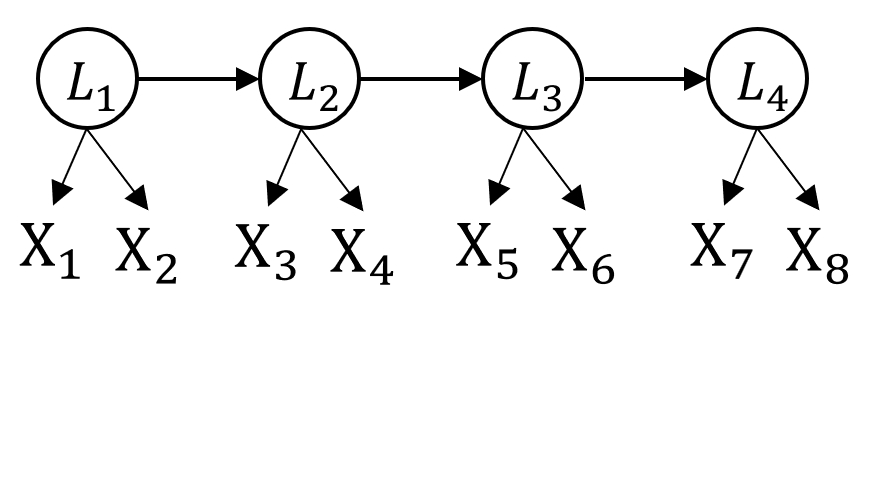
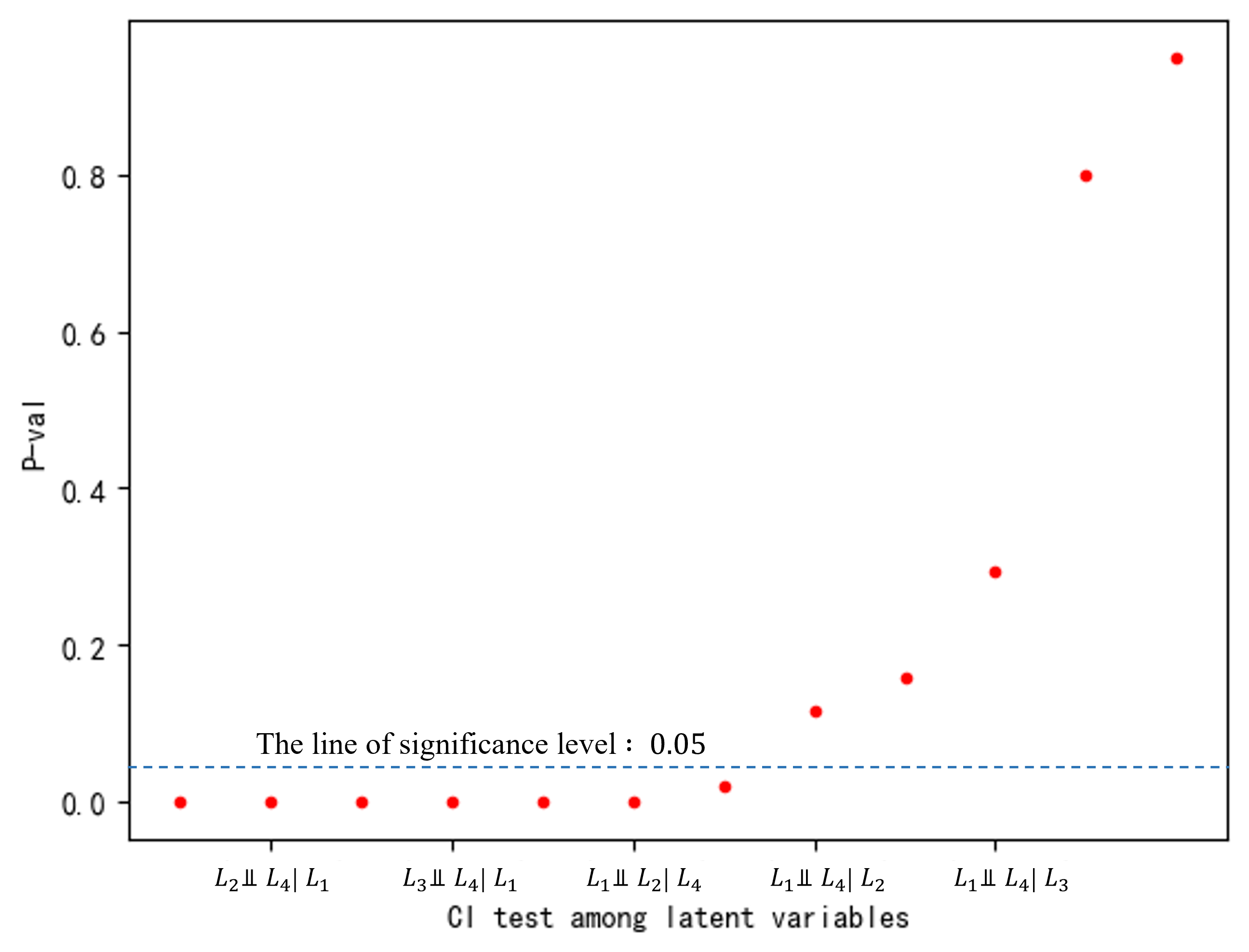
Next, we will show that how the CI relations among latent variables can be distinguished by testing the goodness of fit test. Consider a four latent variables structure as shown in Fig. 8, a chain structure among four latent variables in which each latent variable has two pure observed variables. The data generation process follows the discret LSM model (see the description in the simulation studies section) and the sample size is . We check the CI relations between any given . The results are reported in the right side of 8, in which each red point represents a CI test result, e.g., the second point in the graph represent to test by examining . One can see that the p-value returned by the goodness of fit test is lower than 0.05, which means that we will tend to reject the null hypothesis, i.e., . By sorting all CI test results, one can see that the true CI relations can be identified by setting the significant level to be 0.05.
Appendix H More Experimental Results
In this section, we provide the information required to reproduce our results reported in the main text. We further conduct additional simulation experiments to validate the efficiency of the proposed algorithm (Appendix E).
We first give a details definition of evaluation metrics. Specifically, the performance of causal cluster is evaluated by following scores for the output model from each algorithm, where the true graph is labelled :
-
•
latent omission, the number of latents in that do not appear in divided by the total number of true latents in ;
-
•
latent commission, the number of latents in that could not be mapped to a latent in divided by the total number of true latents in ;
-
•
mismeasurement, the number of observed variables in that are measuring at least one wrong latent divided by the number of observed variables in ;
Moreover, we use the following metric to evaluate the performance of causal structure among latent variables:
-
•
edge omission (EO), the number of edges in the structural model of that do not appear in divided by the possible number of edge omissions;
-
•
edge commission (EC), the number of edges in the structural model of that do not exist in divided by the possible number of edge commissions;
-
•
orientation omission (OO), the number of arrows in the structural model of that do not appear in divided by the possible number of orientation omissions in ;
These evaluation indicators are derived from [1].
Next, we give a concrete implementation of baseline methods.
BayPy: The Bayesian Pyramid Mode (BayPy) is a discrete latent variable structure learning method that assumes the latent structure is a pyramid structure and the latent variable is binary. We use the implementation of [25]. We set the iteration parameter to 1500 and set the search upper bound of the number of latent variables to 5.
LTM: The latent tree model, is a classic method for learning gaussian or binary latent tree structure. We use the implementation from [35]. Specifically, we use the Recursive Grouping (RG) Algorithm in [35] (since it has better performance), and use the discrete information distance to learn the structure of the discrete LSM model.
BPC: The Building Pure Cluster (BPC) algorithm [1] is a classic causal discovery method for the linear latent variable model. We use the implementation from the Tetrad Project package 222https://github.com/cmu-phil/tetrad.
Non-negative CP decomposition: To perform non-negative CP decomposition in our algorithm, we use the implementation from the python package, tensorly 333https://github.com/tensorly/tensorly, and set the maximum iteration parameter to 1000, the cvg criterion parameter to "rec_error".
Data Generation: To generate the probability contingency table or conditional probability contingency table for latent variables and observed variables in our simulation studies, we use the implementation from the python package, pgmpy 444https://github.com/pgmpy/pgmpy. The package provides the function to generate observed data according to the probability contingency table.
Finally, we aim to demonstrate the correctness of our methods in handling cases involving latent variables with varying state spaces. Specifically, we consider the structure model with star structure and the structure, and the measurement model with . The data generation process follows the description in the main context and we let the support of latent variable to be and the support of latent variable to be , for simulating the case that latent variable has different latent support. Besides, the support of the observed variable is . In our implementation, the significant levels for testing the rank of the matrix and tensor are set to 0.005 and 0.05, respectively. The coefficient of probability contingency tables is generated randomly, ranging from , constraining the sum of them to be one.
The results are presented in Table 4 and Table 5. The performance of our method appears superior in scenarios where latent variables have differing state spaces. This improvement is attributed to the reduction in the frequency of higher-order tensor rank testing, facilitated by evaluating the consistency of ranks such as . In contrast, the BayPy approach underperforms in latent structure learning, likely due to its assumption of a pyramid structure with a top-down directionality and no peer-level connections among latent variables. Additionally, the Latent Tree Model (LTM) shows weaker performance in cluster learning, possibly because it was originally designed to handle only binary discrete variables.
| Latent omission | Latent commission | Mismeasurements | |||||||||||
|---|---|---|---|---|---|---|---|---|---|---|---|---|---|
| Algorithm | Our | BayPy | LTM | BPC | Our | BayPy | LTM | BPC | Our | BayPy | LTM | BPC | |
| 5k | 0.09(3) | 0.20(4) | 0.23(5) | 0.96(10) | 0.00(0) | 0.20(4) | 0.00(0) | 0.00(0) | 0.03(1) | 0.18(4) | 0.23(5) | 0.00(0) | |
| 10k | 0.06(2) | 0.17(3) | 0.13(4) | 0.96(10) | 0.00(0) | 0.15(3) | 0.00(0) | 0.00(0) | 0.00(0) | 0.15(3) | 0.13(4) | 0.00(0) | |
| 50k | 0.00(0) | 0.13(3) | 0.10(3) | 0.93(10) | 0.00(0) | 0.15(3) | 0.00(0) | 0.00(0) | 0.00(0) | 0.13(3) | 0.10(3) | 0.00(0) | |
| 5k | 0.12(3) | 0.33(7) | 0.55(10) | 0.96(10) | 0.00(0) | 0.30(6) | 0.00(0) | 0.00(0) | 0.06(2) | 0.30(7) | 0.55(10) | 0.00(0) | |
| 10k | 0.06(2) | 0.26(5) | 0.50(10) | 0.93(10) | 0.00(0) | 0.20(5) | 0.00(0) | 0.00(0) | 0.00(0) | 0.19(5) | 0.50(10) | 0.00(0) | |
| 50k | 0.03(1) | 0.20(4) | 0.50(10) | 0.93(10) | 0.00(0) | 0.15(4) | 0.00(0) | 0.00(0) | 0.00(0) | 0.11(4) | 0.50(10) | 0.00(0) | |
| Edge omission | Edge commission | Orientation omission | |||||||||||
|---|---|---|---|---|---|---|---|---|---|---|---|---|---|
| Algorithm | Our | BayPy | LTM | BPC | Our | BayPy | LTM | BPC | Our | BayPy | LTM | BPC | |
| 5k | 0.00(0) | 1.00(10) | 0.26(8) | 1.00(10) | 0.10(1) | 0.00(0) | 0.00(0) | 0.00(0) | 0.10(1) | 1.00(10) | – | 1.00(0) | |
| Star+ | 10k | 0.00(0) | 1.00(10) | 0.23(6) | 1.00(10) | 0.00(0) | 0.02(1) | 0.0(0) | 0.00(0) | 0.00(0) | 1.00(10) | – | 1.00(0) |
| 50k | 0.00(0) | 1.00(10) | 0.10(3) | 1.00(10) | 0.00(0) | 0.00(0) | 0.00(0) | 0.00(0) | 0.00(0) | 1.00(10) | – | 1.00(0) | |
| 5k | 0.15(3) | 1.00(10) | 0.16(6) | 1.00(10) | 0.10(1) | 0.00(0) | 0.00(0) | 0.00(0) | 0.00(0) | 0.00(0) | – | 0.00(0) | |
| 10k | 0.05(1) | 1.00(10) | 0.13(4) | 1.00(10) | 0.01(1) | 0.00(0) | 0.00(0) | 0.00(0) | 0.00(0) | 0.00(0) | – | 0.00(0) | |
| 50k | 0.00(0) | 1.00(10) | 0.10(3) | 1.00(10) | 0.00(0) | 0.00(0) | 0.00(0) | 0.00(0) | 0.00(0) | 0.00(0) | – | 0.00(0) | |
Appendix I More Details of Real-world Dataset
For the political efficacy data [36], by identifying the support of latent variable to be two, one can identify the causal cluster , . These clusters correspond to the latent variables ’EFFICACY’ and ’RESPONSE’, respectively. In our implementation, we set the significance level to 0.0015. The result is aligned with the ground truth provided in [37].
For the depress dataset, the ground truth structure [37] includes three latent factors: Self-esteem, Depression, and Impulsiveness, with the corresponding observed clusters:
-
•
;
-
•
;
-
•
.
In our implementation, we utilize a bootstrapping resampling approach to enhance the statistical properties of the data. Following the extended results outlined in Appendix E, we first identify the dimension of support for the factors Self-esteem and Depression as four, and set the dimension of support for Impulsiveness at three. The significance level is set to 0.025. The results of our algorithm are presented as follows.
-
•
;
-
•
;
-
•
.
One can see that our algorithm can learn three causal clusters corresponding to three latent factors. Such a result shows that our method finds all latent variables from the depress data. In the latent structure learning process, the PC-TENSOR-RANK algorithm outputs the fully connected graph of the three latent factors, indicating the absence of conditional independence (CI) relations between them. One possible reason is there may be more potential factor interaction structure [44].