Entropy and thermodynamical stability of white dwarfs

Jiří Adam, Jr.***Corresponding authorE-mail address: adam@ujf.cas.cz Institute of Nuclear Physics ASCR, CZ–250 68 Řež, Czech Republic    Emil TruhlíkE-mail address: truhlikemil@gmail.com Institute of Nuclear Physics ASCR, CZ–250 68 Řež, Czech Republic
Abstract

A structure of spherical white dwarfs is calculated for a non-zero temperature. It is shown that the thermodynamical stability of the white dwarf stars can be described naturally within the concept of the Helmholtz free energy of the Coulomb fully ionized electron-ion plasma.

Entropy; Thermodynamics; Stability; White dwarfs
pacs:
23.40.Bw; 14.60.Cd; 67.85.Lm; 97.10.Ld; 97.20.Rp

I Introduction

Description of the white dwarf stars (WDs) often starts from the equation of equilibrium in the Newtonian approximation, without the rotation and the magnetic field included SC1 ; MC §§§The importance of the general relativity for a star with the mass $M$ and the radius $R$ is given by a compactness parameter $x_{g}$ AYP , $$x_{g}\,=\,r_{g}/R\,,\,\,\,r_{g}\,=\,2\mathrm{G}M/c^{2}\,\approx\,2.95\,M/M_{\odot}\,,$$ (1) where $r_{g}$ is the Schwarzschild radius and $M_{\odot}$ is the mass of the Sun. If one takes for $M$ the Chandrasekhar - Landau limit mass SC2 ; LDL $M\,\approx\,1.4\,M_{\odot}$ and the radius $R\,\approx\,5\times 10^{3}$ km, one obtains $x_{g}\,<<\,1$. However, the effects od the general relativity are important for stabilizing very massive and fast rotating WDs SLSSAT .,

$$\frac{d\,P}{d\,r}\,=\,-\frac{\mathrm{G}\,M(r)}{r^{2}}\,\rho\,,\,\,\,\frac{d\,M(r)}{d\,r}\,=\,4\,\pi\,r^{2}\,\rho\,,$$ (2)

from which it follows,

$$\frac{1}{r^{2}}\,\frac{d}{d\,r}\left(\frac{r^{2}}{\rho}\,\frac{d\,P}{d\,r}\right)\,=\,-4\,\pi\,\mathrm{G}\,\rho\,,$$ (3)

where $P$ is the pressure, $\rho$ is the mass density and G is the Newton gravitational constant. One gets explicitly from (3),

$$\frac{1}{\rho}\,\frac{d^{2}\,P}{d\,r^{2}}\,+\,\frac{2}{\rho\,r}\,\frac{d\,P}{d\,r}\,-\,\frac{1}{\rho^{2}}\,\frac{d\,P}{d\,r}\,\frac{d\,\rho}{d\,r}\,+\,4\,\pi\,\mathrm{G}\,\rho\,=\,0\,.$$ (4)

If $P$ as a function of $\rho$ (i.e., the equation of state (EoS)) is known, the equation above can be cast into a second order differential equation for the function $\rho(r)$.

For instance, it was shown in SC1 that writing the EoS in the form

$$P\,=\,\mathrm{K}\,\rho^{(1+\frac{1}{n})}\,,$$ (5)

and $\rho$ as

$$\rho\,=\,\mathrm{\lambda_{c}}\,\theta^{n}\,,$$ (6)

one gets EoS eq. (5) in the form,

$$P\,=\,\mathrm{K}\,\mathrm{\lambda_{c}}^{(1+\frac{1}{n})}\,\theta^{(1+n)}\,,$$ (7)

and from eq. (4) it then follows the famous Lane-Emden (LE) equation,

$$\frac{1}{\xi^{2}}\,\frac{d}{d\,\xi}\,\left(\xi^{2}\,\frac{d\,\theta}{d\,\xi}\right)\,=\,0,$$ (8)

where

$$\xi\,=\,\frac{r}{a}\,,\,\,\,\,a\,=\,\sqrt{\frac{(n+1)}{4\,\pi}\,\frac{\mathrm{K}}{\mathrm{G}}\,\mathrm{\lambda_{c}}^{(\frac{1}{n}-1)}}\,.$$ (9)

Further, if $\mathrm{\lambda_{c}}\,=\,\rho_{c}$, where $\rho_{c}\,=\,\rho(0)$, then $\theta(0)\,=\,1$ and $\left(\frac{d\,\theta}{d\,\xi}\right)\big{|}_{\xi=0}\,=\,0$.

Eq. (8) was discussed in detail in SC1 , where it was shown that for $n\,=\,0,1,5$ one gets explicit solutions. The model with the EoS (7), known as polytropic model, has been frequently used in the astrophysics, in particular for treating the structure of WDs. In this case, the star is considered as a dense Coulomb plasma of nuclei in a charge compensating background of degenerate electron Fermi gas, where the electron - ion interaction is taken in this polytropic approximation. However, for studying the WDs structure, the polytropic model is of restricted use, because it fairly approximates the equation of state only in the extreme non-relativistic limit for $\lambda_{c}\,<<\,10^{6}$ g/cm3 (with $n$ = 3/2) and in the extreme relativistic limit for $\lambda_{c}\,>>\,10^{6}$ g/cm3 (with $n$ = 3). Recall that for $n$ = 3 the mass of the WDs is uniquely given by the Chandrasekhar - Landau limit mass SC2 ; LDL .

Another problem with the polytropic model is its stability. As discussed at length in JPM , the squared Brunt-Väisälä frequency $N^{2}\,=\,0$ in this model. Only if $N^{2}\,>\,0$, the fluid is stable, if $N^{2}\,<\,0$, it is convectively unstable. So the fluid described by the polytropic model is only neutrally stable. According to Ref. JPM , no magnetic equilibrium exists in this case.

Stable stratification has an important influence on stellar magnetic equilibria and their stability. As discussed at length in Ref. TARMM , the study of the magnetic equilibria in stable stratified stars has a long story. It follows from these studies that simple magnetic field configurations are always unstable. In their study, the authors of Ref. TARMM constructed simple analytic models for axially symmetric magnetic fields, compatible with hydromagnetic equilibria in stably stratified stars, with both poloidal and toroidal components of adjustable strength, as well as the associated pressure, density and gravitational potential perturbations, which maked them possible to study directly their stability. It turned out that the instability of toroidal field can be stabilized by a poloidal field containing much less energy than the former, as given by the condition $E_{\mathrm{pol}}/E_{\mathrm{tor}}\,\gtrsim\,2aE_{\mathrm{pol}}/E_{\mathrm{grav}}$, where $E_{\mathrm{pol}}$ and $E_{\mathrm{tor}}$ are the energies of the poloidal and toroidal fields, respectively and $E_{\mathrm{grav}}$ is the gravitational binding energy of the star. It was found in TARMM that $a\approx 7.4$ for main-sequence stars, which compares with $a\approx 10$ obtained by Braithwaite JB , using the method of numerical simulations. But the results for the neutron stars differ by a factor of $\approx$ 4.

The possibility of compensation of instabilities of toroidal fields by a relatively weak poloidal field was earlier studied by Spruit HCS .

As to the instabilities in the poloidal field, stable stratification is of less help for eliminating them TARMM . A relatively stronger toroidal field would be needed in order to stabilize it JB .

As it follows from the discussion in Ch. 3 of the monograph CSBK , the necessary and sufficient condition for the thermodynamical stability of stars with optically thick media is the positive gradient of the entropy,

$$\frac{d\,S}{d\,r}\,>\,0\,.$$ (10)

Respecting this criterion of the stability, the authors of Ref. JPM considered the star as a chemically uniform, monoatomic, classical ideal gas, described in the polytropic model with the EoS (5) as $P\,\sim\,\rho^{\gamma}$, where $\gamma\,=\,4/3\,=\,1\,+\,1/n\,\,\,(n\,=\,3)$ and with the specific entropy

$$s\,\approx\,ln(P/\rho^{\Gamma})\,+\,const\ ,\qquad{\rm where}\quad\Gamma\,=\,\left(\frac{\partial\,P}{\partial\,ln\,\rho}\right)_{ad}\,=\,\frac{5}{3}\ ,$$

for which it holds

$$\frac{d\,s}{d\,r}\,>0\ .$$

In this model, applied to the Ap stars, the constructed magnetic equilibrium turns out to be stable. However, for $\gamma\,=\,5/3\,\,\,(n\,=\,3/2)$, one obtains $\gamma\,=\,\Gamma$, $d\,s/d\,r\,=\,0$ and the magnetic equilibrium is unstable. Similar calculations have recently been done in Ref. LB .

This model cannot be applied to the study of WDs, because they consist of plasma containing the mix of the fully ionized atoms and of the fully degenerate electron gas.

The polytropic model was used to describe super - Chandrasekhar strongly magnetized WDs (SMWDs) in Refs. UDM1 ; UDM2 ; UDM3 and also in Ref. BB . It was shown in BB , that axisymmetric configurations with the poloidal or toroidal fields are unstable and it was concluded that the long lived super - Chandrasekhar SMWDs are unlikely to occur in nature.

In Ref. DC , the authors developed a detailed and self - consistent numerical model with a poloidal magnetic field in the SMWDs. In their model, the rotation, the effects of general relativity and a realistic EoS were taken into account and extensive stability analysis of such objects was performed. As a result, it was found that the SMWDs could potentially exist, but their stability would be mainly limited by the onset of the electron capture and of the picnonuclear reactions. However, it should be noted that the condition of the thermodynamical stability (10) was not checked in Ref. DC .

In the recent paper NCLP , the authors have studied the influence of the electron capture on the stability of the WDs. They used the EoS in the polytropic form (5) in the ultrarelativistic limit $P\,\approx\,K_{0}\,\rho^{4/3}$, with $A$ and $Z$ dependent constant $K_{0}$. Besides, the electrostatic correction and the correction due to the electron-ion interaction are also included in $K_{0}$. This allowed them to calculate the threshold density $\rho_{\beta}$ for the capture of electrons and to set the lower bound for the radius of the WDs. It was also found that the electron capture reduces the mass of WDs by 3 - 13% . Solving the Einstein - Maxwell equations, with the magnetism of the dense matter included, has shown that the magnetized WDs with the polar magnetic field stronger than $10^{13}$ G could be massive enough to explain overluminous type Ia supernova. It was also found that the pure poloidal magnetic field is unstable. Actually, this result follows from the fact that the polytropic model is only neutrally stable, as it has already been discussed above.

In Ref. LB1 , the authors investigated the evolution of isolated massive, highly magnetized and uniformly rotating WDs, under angular momentum loss driven by magnetic dipole braking. They computed general relativistic configurations of such objects using the relativistic Feynman - Metropolis - Teller equation of state for the WD matter. One of the interesting results is obtained for rotating magnetized WD with the mass which is not very close to the non - rotating Chandrasekhar - Landau mass. Such a WD evolves slowing down and behaving as an active pulsar of the type of soft gamma - repeater and anomalous X - ray pulsar MM ; IB ; KBLI ; JAR ; JGC ; RVL ; VBB ; TRM . Let us note that it is not clear if the condition of the thermodynamical stability (10) is fulfilled in Ref. LB1 .

Realistic model of stars as systems of magnetized fully - ionized plasma has been developed in CP - ASJ . In the model, considered in CP - PC3 , an analytical EoS is derived from the Helmholtz free energy of the system of magnetized fully - ionized atoms and of the degenerate electron gas, whereas, in ASJ also positrons were included. Such an EoS covers a wide range of temperatures and densities, from low-density classical plasmas to relativistic, quantum plasma conditions.

Starting in Sect. II.1 from the equation of equilibrium (4), and using in Sect. II.2 the function $P(\rho)$, obtained from the EoS mentioned above, we get the second order equation for the matter density $\rho$. Solving this equation, we study the structure of corresponding WDs for a representative series of values of the central density $\rho_{c}$, chosen from the interval $10^{4}\,\mathrm{g/cm^{3}}\,<<\,\rho_{c}\,<<\,2\times\,10^{9}\,\mathrm{g/cm^{3}}$, and simultaneously using the electron and ion entropies from Sects. III.1 and III.2, we show that the criterion of the thermodynamical stability (10) is fulfilled in all cases (see FIG. 2 and FIG. 3). Besides, using LE eq.(8), we calculate for comparison for the extreme non - relativistic and extreme relativistic values of $\rho_{c}$ the mass and radius of corresponding WDs, which are presented in TABLE I.

In Appendix A, we discuss different ways of calculating the structure of WDs and summarize relations for the scaling parameter $\mathrm{a_{s}}$ and for the LE approximation. In Appendix B, we express the functions $f_{1}$ and $f_{2}$, entering the pressure $P(\rho)$ in terms of the Fermi - Dirac integrals and in Appendix C, we briefly describe how to decompose the thermodynamical quantities for free electrons into series in powers of $k_{\mathrm{B}}T/\tilde{E}_{F}$, where $\tilde{E}_{F}=\mu_{\mathrm{e}}(T=0)$ is the Fermi energy with the rest mass contribution subtracted.

Our results show that the realistic model developed in CP - ASJ is a good starting model to be applied to construct the WDs with stable magnetic fields.

II Methods and input

II.1 Modified equation of stability

Let us write eq. (4) in the form,

$$\frac{d^{2}\,P}{d\,r^{2}}\,+\,\frac{2}{r}\,\frac{d\,P}{d\,r}\,-\,\frac{1}{\rho}\,\frac{d\,P}{d\,r}\,\frac{d\,\rho}{d\,r}\,+\,4\,\pi\,\mathrm{G}\,\rho^{2}\,=\,0\,.$$ (11)

Considering now the pressure $P$ as a function (solely) of the density $\rho$, eq. (11) can be transformed into the 2nd order differential equation for $\rho$,

$$\frac{d^{2}\,\rho}{d\,r^{2}}\,+\,f_{1}(\rho)\,\left(\frac{d\,\rho}{d\,r}\right)^{2}\,+\,\frac{2}{r}\,\frac{d\,\rho}{d\,r}\,+\,\frac{4\,\pi\,\mathrm{G}}{f_{2}(\rho)}\,\rho^{2}\,=\,0\,,$$ (12)

where

$$f_{1}(\rho)\,=\,\left(\frac{d^{2}\,P}{d\,\rho^{2}}\right)\bigg{/}\left(\frac{d\,P}{d\,r}\right)\,-\,\frac{1}{\rho}\,,\,\,\,\,\,f_{2}(\rho)\,=\,\frac{d\,P}{d\,\rho}\,.$$ (13)

Next we set

$$r\,=\,\mathrm{a_{s}}\,x\,,\,\,\,\rho\,=\,\lambda_{c}\,y\,.$$ (14)

If $\lambda_{c}$ is the matter density in the center of the star $\lambda_{c}=\rho(0)$, then

$$y(0)\,=\,0\,,\,\,\,\frac{d\,y}{d\,r}\big{|}_{0}\,=\,0\,.$$ (15)

From relations

$$\frac{dP}{d\rho}\,=\,\frac{dP}{\lambda_{c}\,dy}\,,\,\,\,\frac{d^{2}P}{d\rho^{2}}\,=\,\frac{d^{2}P}{\lambda_{c}^{2}\,dy^{2}}\,,$$ (16)

it follows

$$f_{1}(\rho)\,=\,\frac{1}{\lambda_{c}}\,f_{1}(y)\,,\,\,\,f_{2}(\rho)\,=\,\frac{1}{\lambda_{c}}\,f_{2}(y)\,.$$ (17)

Then, in terms of the new variables (14), eq. (12) becomes,

$$\frac{d^{2}\,y}{d\,x^{2}}\,+\,f_{1}(y)\,\left(\frac{d\,y}{d\,x}\right)^{2}\,+\,\frac{2}{x}\,\frac{d\,y}{d\,x}\,+\,\frac{\mathrm{C}}{f_{2}(y)}\,y^{2}\,=\,0\,,$$ (18)

with

$$\mathrm{C}\,=\,4\,\pi\,\mathrm{G}\,\mathrm{a_{s}}^{2}\,\lambda_{c}^{2}\,.$$ (19)

We solved eq. (18) by the standard 4th order Runge-Kutta method for various values of the central matter density $\lambda_{c}$. The choice of the value of the scaling parameter $\mathrm{a_{s}}$ is discussed in Appendix A. In our calculations we use the value (see (70))

$$\mathrm{a}_{s}\,=\,8686.26\,{\rm km}.$$ (20)

II.2 The Helmholtz free energy and the EoS

Here we follow Ref. PC3 , where the Helmholtz free energy $F$ of the plasma is defined as,

$\displaystyle F\,$ $\displaystyle=$ $\displaystyle\,F^{(e)}_{id}\,+\,F^{(i)}_{id}\,+\,F_{ii}\,+\,F_{ee}\,+\,F_{ie}\,,$ (21)
$\displaystyle\simeq$ $\displaystyle F^{(e)}_{id}\,+\,F_{lat}\ ,\quad F_{lat}=\,F^{(i)}_{id}\,+\,F_{ii}\ .$

On the first line, the first two terms correspond to the ideal part of the free energy of ions and electrons, and the last three terms correspond to the ion - ion, electron - electron, and ion - electron interactions, respectively. The second line corresponds to the approximation adopted in this paper: the sum of the 2nd and 3rd terms of the 1st line is denoted as $F_{lat}$ and evaluated as in Ref. PC3 in one - component plasma model (OCP) in the regime of Coulomb crystal. Less important and more uncertain contributions $F_{ee}$ and $F_{ie}$ are skipped. It should be noted that these contributions are less important only in degenerate plasmas. In the non-degenerate regime, they can be of the same order of magnitude as $F_{ii}$, especially if Z is not large PC3 .

Refer to caption
Refer to caption
FIG. 1: Dependence of the electron pressure $P$ $[g/cm\cdot sec^{2}]$ on the matter density $\rho$ $[g/cm^{3}]$ and the temperature $T$ $[K]$. In the upper panel, somewhat wider ranges of densities and temperatures are considered, while in the lower one, they are relevant for the carbon WDs.

The particle density $N$, internal energy $U$, the entropy $S$ and Helmholtz free energy $F$ are related by:

$\displaystyle T\,S$ $\displaystyle=$ $\displaystyle U+P\,V-\mu\,N\ ,$ (22)
$\displaystyle F$ $\displaystyle=$ $\displaystyle U-T\,S=\mu\,N-P\,V\ .$ (23)

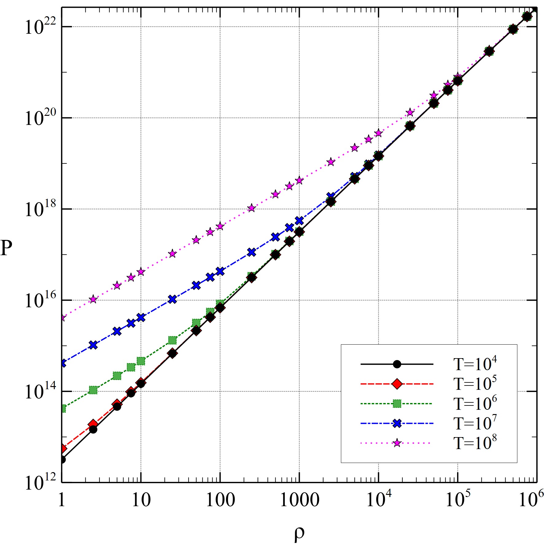
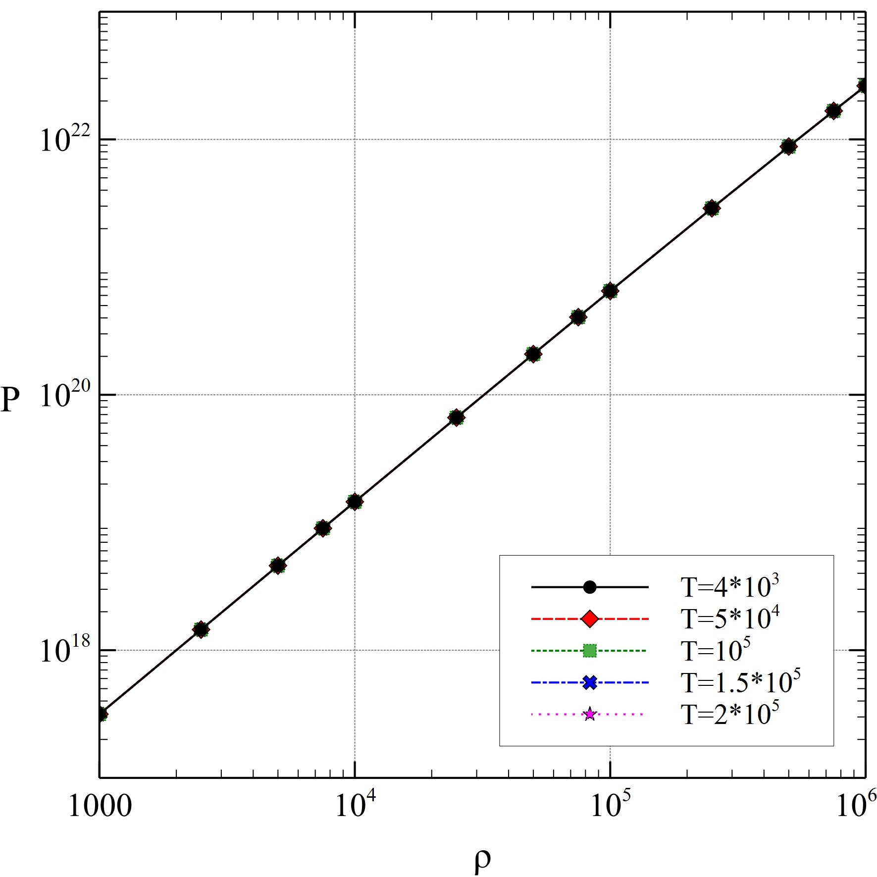
In the lower panel of FIG. 1, we present the dependence of the electron pressure on $\rho$ for various values of $T$ for the carbon WDs with $A\,=\,12\,,\ Z\,=\,6$. In this case, the dependence of the electron presure on the matter density is $T$ - independent Similar $P^{(\mathrm{e})}-\rho$ dependence on various values of $T$ was presented in Fig. 1 of Ref. KB ..

In general, the pressure and the entropy can be calculated from $F$ by:

$$P\,=\,-\left(\frac{\partial\,F}{\partial\,V}\right)_{T}\,,\qquad S\,=\,-\left(\frac{\partial\,F}{\partial\,T}\right)_{V}\ .$$

But for free electrons the number density $n_{\mathrm{e}}$, pressure $P^{(\mathrm{e})}_{id}$ and energy $U$ are known explicitly:

$\displaystyle n_{\mathrm{e}}\,$ $\displaystyle\equiv$ $\displaystyle\frac{N_{e}}{V}=\,\mathrm{c_{n}}\,\big{[}I_{1/2}(\chi_{\mathrm{e}},\tau)+\,\tau\,I_{3/2}(\chi_{\mathrm{e}},\tau)\big{]}\,,$ (24)
$\displaystyle P^{(\mathrm{e})}_{id}\,$ $\displaystyle=$ $\displaystyle\,\mathrm{c_{p}}\,\big{[}I_{3/2}(\chi_{\mathrm{e}},\tau)+\,\frac{\tau}{2}\,I_{5/2}(\chi_{\mathrm{e}},\tau)\big{]}\,,$ (25)
$\displaystyle U^{(\mathrm{e})}_{id}\,$ $\displaystyle=$ $\displaystyle\,\mathrm{c_{e}}\,\big{[}I_{3/2}(\chi_{\mathrm{e}},\tau)+\,\tau\,I_{5/2}(\chi_{\mathrm{e}},\tau)\big{]}\equiv{\cal E}_{e}\,V\,,$ (26)

where $\chi_{\mathrm{e}}\,=\,\mu_{\mathrm{e}}\beta$, $\mu_{\mathrm{e}}$ is the electron chemical potential without the rest energy $m_{\mathrm{e}}c^{2}$ and dimensionless $\tau\,=\,T/T_{\mathrm{r}}\,,$ with $T_{\mathrm{r}}\,=\,m_{\mathrm{e}}\,c^{2}/k_{\mathrm{B}}\,\simeq\,5.9301\times 10^{9}\,\mathrm{K}$ (from the Boltzmann constant $k_{B}\simeq 8.617\times 10^{-11}$MeV/K). In the last relation we introduce the electron energy density ${\cal E}_{e}=U^{(\mathrm{e})}_{id}/V$. Further:

$\displaystyle\mathrm{c_{n}}\,$ $\displaystyle=$ $\displaystyle\,\frac{\sqrt{2}}{\pi^{2}\hbar^{3}}\left(\frac{m_{\mathrm{e}}}{\beta}\right)^{3/2}=3\sqrt{2}\rho_{0}\,\tau^{3/2}\,,\quad\beta\,=\,\frac{1}{k_{\mathrm{B}}T}\ ,\quad\rho_{0}=\frac{1}{3\pi^{2}\,\lambda_{e}^{3}}\ ,$
$\displaystyle\mathrm{c_{p}}\,$ $\displaystyle=$ $\displaystyle\,\frac{(2m_{\mathrm{e}})^{3/2}}{3\pi^{2}\hbar^{3}\beta^{5/2}}=2\sqrt{2}\,m_{e}c^{2}\,\rho_{0}\,\tau^{5/2}\ ,$
$\displaystyle\mathrm{c_{e}}=\frac{3}{2}\mathrm{c_{p}}\,$ $\displaystyle=$ $\displaystyle\,\frac{\sqrt{2}\,m_{\mathrm{e}}^{3/2}}{\pi^{2}\hbar^{3}\beta^{5/2}}=3\sqrt{2}\,m_{e}c^{2}\,\rho_{0}\,\tau^{5/2}\ ,$

where $\lambda_{e}$ is the electron Compton length (69).

The generalized (relativistic) Fermi-Dirac integrals $I_{\nu}(\chi_{\mathrm{e}}\,,\,\tau)$ are defined as follows:

$$I_{\nu}(\chi_{\mathrm{e}},\tau)\,=\,\int\limits_{0}^{\infty}\frac{x^{\nu}(1\,+\,\tau x/2)^{1/2}}{e^{(x\,-\,\chi_{\mathrm{e}})}\,+\,1}\mathrm{d}x\,.$$ (27)

The functions $f_{1}(y)$ and $f_{2}(y)$ of previous section are presented in terms of the Fermi - Dirac integrals $I_{\nu}(\chi_{\mathrm{e}}\,,\,\tau)$ in Appendix B.

One obtains the EoS by referring to the neutrality of the plasma, which provides the equation between the mass density $\rho$ of the ion and the electron number density $n_{\mathrm{e}}$,

$$n_{\mathrm{e}}\,=\,Zn_{i}\,=\,\frac{Z\rho}{Am_{u}}=\frac{\rho}{\mu_{u}}\,,$$ (28)

where $Z$ is the ion charge number, $A$ is the mass number, $n_{i}$ is the ion number density,
$m_{u}$ is the atomic mass unit and $\mu_{u}=A\,m_{u}/Z$ is introduced in (68). Given values of $A\,,Z$ and $\rho$ one gets $n_{e}$ from the neutrality condition (28) and then reversing eq. (24) for a given temperature $T$, obtains the value of $\chi_{\mathrm{e}}$. Substituting this $\chi_{\mathrm{e}}$ into eq. (25), one gets the value of the electron pressure $P^{(\mathrm{e})}_{id}$ corresponding to the given value of $\rho$.

Table 1: In the upper part of this table we present the results of calculations of the radii and masses of the WDs for representative values of the central mass densities $\lambda_{c}$. We have solved the equation of stability (18) with the scaling parameter $a_{s}$ of eq. (20). The EoS is obtained within the concept of the Helmholtz free energy of the Coulomb plasma, using eqs. (25), (24) and (28). The central fractional Fermi momentum eq. (34) $x_{rc}$ is also listed, since it indicates whether the dynamics is non-relativistic or relativistic. In the lower part of the table (below the middle double line) we present the radii and masses obtained from the LE eq. (8), which is based on the polytropic EoS eq. (7). $R_{0}$ and $M_{0}$ are radii and masses in this approximation, $r_{0}$ and $m_{0}$ the corresponding dimensionless quantities, introduced at the end of Appendix A in eqs. (78-80) and (81-83). Comparing these (LE) results with our numerical ones (which do not employ a polytropic EoS) one can see that they are close to each other in the non-relativistic case, but in the relativistic regime they approach each other only in the extreme relativistic limit of very large densities.
model 1 2 3 4 5 6
$\lambda_{c}[g/cm^{3}]$ $10^{4}$ $10^{5}$ $10^{6}$ $10^{7}$ $10^{8}$ $2\cdot 10^{9}$
$x_{rc}$ $0.173$ $0.372$ $0.801$ $1.36$ $3.72$ $10.1$
$R_{WD}$ [km] $2.40\cdot 10^{4}$ $1.63\cdot 10^{4}$ $1.09\cdot 10^{4}$ $7.04\cdot 10^{3}$ $4.30\cdot 10^{3}$ $2.05\cdot 10^{3}$
$M/M_{\odot}$ 0.048 0.146 0.391 0.816 1.15 1.37
n $3/2$ $3/2$ 3 3 3
$r_{0}$ $2.78$ $1.90$ $1.79$ $0.830$ $0.306$
$m_{0}$ $0.0185$ $0.0583$ $0.542$ $0.542$ $0.542$
$R_{0}$ [km] $2.42\cdot 10^{4}$ $1.65\cdot 10^{4}$ $1.55\cdot 10^{4}$ $7.21\cdot 10^{3}$ $2.66\cdot 10^{3}$
$M_{0}/M_{\odot}$ 0.050 0.157 1.46 1.46 1.46

Apart from the electron pressure, Chamel and Fantina CHFA have taken into account also the lattice pressure $P_{\mathrm{lat}}$, derived from the dominant static-lattice (Madelung) part of the ion free energy PC3 , i.e. approximating $F_{lat}\simeq F_{M}$:

$$F_{\mathrm{M}}\,=\,N_{i}k_{B}T\mathrm{C}_{\mathrm{M}}\,\Gamma\,,\quad N_{i}\,=\,n_{i}V\ ,$$ (29)

and for the bcc crystal the Madelung constant is BPY :

$\displaystyle\mathrm{C}_{\mathrm{M}}$ $\displaystyle=$ $\displaystyle-0.89592925568\,.$ (30)

The ion coupling parameter

$$\Gamma\,=\,\frac{(Ze)^{2}}{a_{i}k_{\mathrm{B}}T}\,,$$ (31)

is given in terms of the ion sphere radius $a_{i}\,=\,\big{(}\frac{4}{3}\pi n_{i}\big{)}^{-1/3}$.

As it can be seen from Table III CHFA , the effect of the pressure $P_{\mathrm{lat}}$ on the mass of the WDs containing the light elements is only few percents and we do not take it into account.

The results of comparative calculations are presented in Table 1.

III Entropy and its gradient in WDs

In this section we calculate one - electron and ion entropies and their gradients within the above introduced Coulomb plasma theory based on the Helmholtz free energy concept. We show on the representative set of WDs that both entropies are positive and that their gradients satisfy the condition of the thermodynamical stability, required by eq. (10). We will deal with a reduced dimensional entropy defined (both for electrons and ions) as:

$\displaystyle\hat{s}$ $\displaystyle=$ $\displaystyle\frac{S}{k_{B}\,N}\ ,$ (32)

where $N$ is a number of particles and $k_{\mathrm{B}}$ is the Boltzman constant. We will evaluate and plot a derivative of various contributions to this reduced entropy in respect to the dimensionless radius $x$ (see (14)), i.e., $d\hat{s}/d\,x$.

III.1 The electron entropy

For the free electrons it follows from (32) and relations (24-26):

$\displaystyle\hat{s}_{e}$ $\displaystyle=$ $\displaystyle\frac{1}{k_{\mathrm{B}}T}\frac{U^{(e)}_{id}+P^{(e)}_{id}\,V-N_{e}\,\mu_{e}}{V\,n_{e}}=\frac{1}{k_{\mathrm{B}}T}\,\left(\frac{{\cal E}_{e}+P^{(e)}_{id}}{n_{e}}-\mu_{e}\right)$ (33)
$\displaystyle=$ $\displaystyle\frac{5\,I_{3/2}(\chi_{e},\tau)+4\tau\,I_{5/2}(\chi_{e},\tau)}{3(I_{1/2}(\chi_{e},\tau)+\tau\,I_{3/2}(\chi_{e},\tau))}-\chi_{e}\simeq\pi^{2}\,\tau\,\frac{\epsilon_{F}}{x^{2}_{\mathrm{r}}}\,,$

where $n_{\mathrm{e}}$ is the electron density, $\tau\,=\,T/T_{\mathrm{r}}$, $T_{\mathrm{r}}\,=\,m_{\mathrm{e}}c^{2}/k_{\mathrm{B}}$. Further, $p_{\mathrm{F}}\,=\,\hbar(3\pi^{2}n_{\mathrm{e}})^{1/3}$ is the electron Fermi momentum and the dimensionless Fermi momentum $x_{r}$ and energy $\epsilon_{F}$ are

$\displaystyle x_{\mathrm{r}}=\frac{p_{\mathrm{F}}}{m_{\mathrm{e}}c}\ ,\quad\epsilon_{F}=\sqrt{1+x^{2}_{\mathrm{r}}}\equiv\tilde{\epsilon}_{F}+1\ .$ (34)

The last equation in eq. (33) is obtained by the Sommerfeld expansion (see Appendix C), it agrees with equation (6) in PC2 . We checked numerically that for our calculations it is sufficient to take the termodynamic quantities in the Sommerfeld approximation (SA).

As for the derivative of the electron entropy in respect to the dimensionless WD radius $x$, let us first consider it in a more transparent SA. Using the charge neutrality of the plasma (28), the electron Fermi momentum can be connected to the matter density $\rho$ as follows,

$$p_{\mathrm{F}}\,=\,\hbar\,\bigg{(}\frac{3\pi^{2}\rho}{\mu_{u}}\bigg{)}^{1/3}\equiv D\,\rho^{1/3}\ ,\quad D\,=\,\hbar\bigg{(}\frac{3\pi^{2}}{\mu_{u}}\bigg{)}^{1/3}\,.$$ (35)

Since $\rho$ is decreasing to the surface of the WD, $p_{\mathrm{F}}$ and $x_{\mathrm{r}}$ are also decreasing, and it follows from eq. (33) that $\hat{s}_{\mathrm{e}}$ is increasing. In other words, the specific one-electron entropy is stratified. With the help of relations:

$$x_{r}=\frac{D}{m_{e}c}\,\rho^{1/3}\ ,\qquad\epsilon_{F}=\frac{\sqrt{(m_{\mathrm{e}}c)^{2}\,+\,D^{2}\rho^{2/3}}}{m_{e}c}\ ,$$

the electron entropy (33) can be transformed to the form, suitable for calculations,

$$\hat{s}_{\mathrm{e}}\,=\,\frac{\pi^{2}k_{\mathrm{B}}T}{cD^{2}\rho^{2/3}}\,\sqrt{(m_{\mathrm{e}}c)^{2}\,+\,D^{2}\rho^{2/3}}\,,$$ (36)

It is convenient to write the gradient of $\hat{s}_{\mathrm{e}}$ as a product:

$\displaystyle\frac{d\hat{s}_{\mathrm{e}}}{dx}\,$ $\displaystyle=$ $\displaystyle\,\left(\rho\,\frac{d\hat{s}_{\mathrm{e}}}{d\rho}\right)\cdot\,\frac{1}{\rho}\frac{d\rho}{dx}\ ,\qquad\frac{1}{\rho}\frac{d\rho}{dx}<0\ ,$ (37)
$\displaystyle\rho\frac{d\hat{s}_{\mathrm{e}}}{d\rho}\,$ $\displaystyle=$ $\displaystyle\,-\frac{\pi^{2}k_{\mathrm{B}}T}{3cD^{2}\,\,\rho^{2/3}}\,\frac{2(m_{\mathrm{e}}c)^{2}+D^{2}\rho^{2/3}}{\sqrt{(m_{\mathrm{e}}c)^{2}\,+\,D^{2}\rho^{2/3}}}=-\frac{\pi^{2}\,\tau}{3}\,\frac{2+x_{r}^{2}}{x_{r}^{2}\,\epsilon^{2}_{F}}<0\ .$ (38)

Obviously, both terms are dimensionless and negative, hence their product is dimensionless and positive:

$$\frac{d\hat{s}_{\mathrm{e}}}{dx}\,>\,0\,.$$ (39)

It should be noted, that our calculations respect the criterion of the strong degeneracy,

$$\theta\,=\,T/T_{\mathrm{F}}\,<<\,1\,,\quad{\rm where}\ T_{\mathrm{F}}\,=\,\frac{\tilde{E}_{\mathrm{F}}}{k_{\mathrm{B}}}\,,$$ (40)

and $\tilde{E}_{\mathrm{F}}=E_{\mathrm{F}}-m_{e}c^{2}=\,c[(m_{\mathrm{e}}c)^{2}\,+\,p^{2}_{\mathrm{F}}]^{1/2}\,-\,m_{\mathrm{e}}\,c^{2}=m_{e}c^{2}\,\tilde{\epsilon}_{\mathrm{F}}$  is the Fermi energy with the rest mass contribution subtracted.

Due to very good termal conductivity of the WD the temperature $T$ (and hence $\tau=T/T_{r}$) are nearly constant inside the WD, with the exception of a thin skip at its surface. Therefore, in our calculations we consider $\tau$ to be independent of the radius $x$.

We have also checked that the empirical factor $(1\,+\,\Delta\tilde{\epsilon}/\tilde{\epsilon})^{-1}$ PC2 , minimizing the numerical jump of the transition between the fit for $\chi_{\mathrm{e}}<14$ and the Sommerfeld expansion for $\chi_{\mathrm{e}}>14$, did not lead in our calculations to any sizeable effect.

Let us now briefly mention equation for the derivative of the electron entropy following from the full form of (33). For easier comparison with equations (37,38) we can again use the factorization (37), where the 2nd term is now (with the help of (24) and (28)):

$\displaystyle\rho\frac{d\hat{s}_{\mathrm{e}}}{d\rho}\,$ $\displaystyle=$ $\displaystyle n_{e}\,\frac{d\hat{s}_{\mathrm{e}}}{dn_{e}}=\frac{n_{e}}{n^{\prime}_{e}}\cdot\,\hat{s}^{\prime}_{e}\ ,$ (41)
$\displaystyle n^{\prime}_{e}$ $\displaystyle\equiv$ $\displaystyle\frac{dn_{e}}{d\chi_{e}}=I^{\prime}_{1/2}+\tau\,I^{\prime}_{3/2}\ ,\qquad I^{\prime}_{\nu}\equiv\frac{d\,I_{\nu}(\chi_{e},\tau)}{d\chi_{e}}\ ,$
$\displaystyle\hat{s}^{\prime}_{e}$ $\displaystyle\equiv$ $\displaystyle\frac{d\hat{s}_{e}}{d\chi_{e}}=\frac{(I_{1/2}+\tau\,I_{3/2})(5I^{\prime}_{3/2}+4\tau I^{\prime}_{5/2})-(I^{\prime}_{1/2}+\tau\,I^{\prime}_{3/2})(5I_{3/2}+4\tau I_{5/2})}{3(I_{1/2}+\tau\,I_{3/2})^{2}}-1\ .$

To calculate (41) one needs derivatives of the Fermi-Dirac integrals $I_{\nu}(\chi,\tau)$ in respect to $\chi$. It is also not obvious from the general equation that (41) is negative. Nevertheless, we checked numerically that in our calculations the general equation (41) agrees very well with the approximate one (38).

III.2 The ion entropy

As for the ions, we consider them in the crystalline phase, in which they are arranged in the body-centered cubic (bcc) Coulomb lattice (see Sect. 3.2.2 of Ref. PC3 ).

In this state, $T<T_{\mathrm{m}}$, where $T_{\mathrm{m}}$ is the melting temperature. For the one-component Coulomb plasma, it is obtained from the relation,

$$\Gamma_{\mathrm{m}}\,=\,2.2747\times 10^{5}\,\frac{Z^{5/3}}{T_{\mathrm{m}}}\,\bigg{(}\rho\frac{Z}{A}\bigg{)}^{1/3}\,,$$ (42)

where $\Gamma_{\mathrm{m}}\,=\,175\,\pm\,0.4$PC1 .

Beyond the harmonic-lattice approximation (29), the reduced dimensionless one-ion free energy is given by:

$\displaystyle f_{\mathrm{lat}}(\Gamma,\eta)$ $\displaystyle\equiv$ $\displaystyle\frac{F_{\mathrm{lat}}}{N_{\mathrm{i}}k_{\mathrm{B}}T}=C_{\mathrm{M}}\,\Gamma\,+\,1.5\,u_{1}\,\eta\,+\,f_{\mathrm{th}}\,+\,f_{\mathrm{ah}}\ .$ (43)

The first three terms describe the harmonic lattice model BPY and $f_{\mathrm{ah}}$ is the anharmonic correction to the Coulomb lattice. Further, $C_{\mathrm{M}}$ is the Madelung constant (30) and
$u_{1}\,=\,0.5113875$. The parameter $\eta$, determining the importance of the quantum effects in a strongly coupled plasma, is PC3 :

$$\eta\,\equiv\,7.835\frac{Z}{A}\cdot\frac{\sqrt{\rho}}{T}\,\times 10^{3}\,.$$ (44)

The ion coupling parameter $\Gamma\sim 1/T$ is defined by (31).

For $f_{\mathrm{th}}$ we adopt the following fitting formula, used in the Appendix B.2 of Ref. PC3 :

$$f_{\mathrm{th}}(\eta)\,=\,\sum_{i=1}^{3}ln\big{(}1-e^{-\alpha_{i}\eta}\big{)}-\frac{A(\eta)}{B(\eta)}\,,$$ (45)

where $\alpha_{1}\,=\,0.932446,\,\alpha_{2}\,=\,0.334547,\,\alpha_{3}\,=\,0.265764$ and

$\displaystyle A(\eta)\,=\,\sum_{i=1}^{7}a_{i}\,\eta^{m_{i}}\ ,\quad B(\eta)\,=\,\sum_{i=1}^{8}b_{i}\,\eta^{n_{i}}\ .$ (46)
Table 2: In this table, the input data for eqs. (46) are presented.
i ai mi bi ni
1 1.0 0 261.66 0
2 0.1839 1 7.07997 2
3 0.593 586 2 4.094 84$\times 10^{-2}$ 4
4 5.4814$\times 10^{-3}$ 3 3.973 55$\times 10^{-4}$ 5
5 5.01813$\times 10^{-4}$ 4 5.11148$\times 10^{-5}$ 6
6 3.9247$\times 10^{-7}$ 6 2.19749$\times 10^{-6}$ 7
7 5.8356$\times 10^{-11}$ 8 1.866985$\times 10^{-9}$ 9
8 - - 2.78772$\times 10^{-13}$ 11

For the anharmonic correction of the Coulomb lattice $f_{\mathrm{ah}}$, we use the anharmonic contribution to the one-ion entropy from the Sect. 4 of the recent work BC .

Using eq. (43), we calculate the dimensionless one-ion entropy as,

$\displaystyle\hat{s}_{i}(\Gamma,\eta)$ $\displaystyle=$ $\displaystyle\,-\frac{1}{k_{\mathrm{B}}\,N_{i}}\,\frac{\partial F_{lat}}{\partial T}\,=\,-\,f_{lat}-T\,\frac{\partial f_{lat}}{\partial T}=-\,f_{lat}+\Gamma\,\frac{\partial f_{lat}}{\partial\Gamma}+\eta\,\frac{\partial f_{lat}}{\partial\eta}\ ,$ (47)

where we used relations

$$T\,\frac{\partial\Gamma}{\partial T}\,=-\Gamma\ ,\quad T\,\frac{\partial\eta}{\partial T}\,=-\eta\ .$$ (48)

It is obvious from (47) that the first two terms of (43) (linear in $\Gamma$ and $\eta$, resp.) do not contribute to the entropy (since the corresponding contributions to $F_{lat}$ do not depend on temperature). From the last part of harmonic contribution, i.e. from $f_{th}$, we obtain for the harmonic part of the entropy $\hat{s}_{i}(har)$ two contributions corresponding to two terms of (45):

$$\hat{s}_{i}(har)\,=\,\hat{s}_{ths}(\eta)\,+\,\hat{s}_{thr}(\eta)\,,$$ (49)

with

$\displaystyle\hat{s}_{ths}(\eta)\,$ $\displaystyle=$ $\displaystyle\,\sum_{k=1}^{3}\,\big{[}-ln(1-e^{-\alpha_{k}\,\eta})\,+\,\frac{\eta\alpha_{k}e^{-\alpha_{k}\,\eta}}{1-e^{-\alpha_{k}\,\eta}}\big{]}\,,$ (50)
$\displaystyle\hat{s}_{thr}(\eta)\,$ $\displaystyle=$ $\displaystyle\,\frac{A(\eta)}{B(\eta)}\,-\,\frac{\tilde{A}(\eta)^{\prime}}{B}\,+\,A(\eta)\,\frac{\tilde{B}(\eta)^{\prime}}{B(\eta)^{2}}\ ,$ (51)

where we denote

$$\tilde{C}(\eta)^{\prime}\,\equiv\,\eta\,\frac{dC(\eta)}{d\eta}\,,\,\,\,\,C\,=\,A\,,B\,.$$ (52)

The anharmonic part of the one-ion entropy $\hat{s}_{i}(ah)$ was parametrized in Ref. BC . From eqs. (20) - (24) of this paper one gets:

$\displaystyle\hat{s}_{i}(ah)\,$ $\displaystyle=$ $\displaystyle\,\frac{\tilde{A}^{S}_{1}(\eta)}{\Gamma}\,+\,\frac{\tilde{A}^{S}_{2}(\eta)}{\Gamma^{2}}\,+\,\frac{\tilde{A}^{S}_{3}(\eta)}{\Gamma^{3}}\,,\qquad\tilde{A}^{S}_{i}(\eta)=\eta^{i}\,A^{S}_{i}(\eta)\,,$ (53)
$\displaystyle\tilde{A}^{S}_{1}(\eta)\,$ $\displaystyle=$ $\displaystyle\,-2A_{11}\,\frac{2A_{12}\eta^{2}\,+\,1}{(1\,+\,A_{12}\eta^{2})^{2}}-2A_{13}\,\frac{2A_{14}\eta^{2}\,+\,1}{(1\,+\,A_{14}\eta^{2})^{2}}\,,$ (54)
$\displaystyle\tilde{A}^{S}_{2}(\eta)\,$ $\displaystyle=$ $\displaystyle\,\frac{3A_{2cl}}{2(1\,+\,A_{21}\eta^{4})^{1/4}}\,,$ (55)
$\displaystyle\tilde{A}^{S}_{3}(\eta)\,$ $\displaystyle=$ $\displaystyle\,\frac{4A_{3cl}}{3}\,.$ (56)

The parameters entering eqs. (54)-(56) are listed in Table 1 and in eqs. (9)-(11)
of Ref. BC :

$\displaystyle A_{1cl}\,=\,10.2\,,\quad A_{2cl}\,=\,248\,,\quad\,A_{3cl}\,=\,2.03\times 10^{5}\,,$
$\displaystyle A_{1q}\,=\,-0.62/6\,,\quad A_{2q}\,=\,-0.56\,,$
$\displaystyle A_{11}\,=\,-10\,,\quad A_{12}\,=\,6\times 10^{-3}\,,\quad A_{13}\,=\,-0.2\,,\quad A_{14}\,=\,0.2167\,,\quad A_{21}\,=\,2.9624\times 10^{-4}\ ,$

As for the derivative of the electron entropy (37), let us also for $\hat{s}_{i}$ factorize:

$\displaystyle\frac{d\hat{s}_{\mathrm{i}}}{dx}\,$ $\displaystyle=$ $\displaystyle\,\left(\rho\,\frac{d\hat{s}_{\mathrm{i}}}{d\rho}\right)\cdot\,\frac{1}{\rho}\frac{d\rho}{dx}\ ,\qquad\frac{1}{\rho}\frac{d\rho}{dx}<0\ .$ (57)

Then, using the fact that $\hat{s}_{i}=\hat{s}_{i}(\Gamma,\eta)$ and taking into account the identities:

$$\rho\,\frac{\partial\Gamma}{\partial\rho}\,=\frac{\Gamma}{3}\ ,\quad\rho\,\frac{\partial\eta}{\partial\rho}\,=\frac{\eta}{2}\ ,$$ (58)

we get for the ion entropy:

$\displaystyle\rho\,\frac{d\hat{s}_{i}}{d\rho}$ $\displaystyle=$ $\displaystyle\rho\,\frac{\partial\Gamma}{\partial\rho}\,\frac{\partial\hat{s}_{i}}{\partial\Gamma}+\rho\,\frac{\partial\eta}{\partial\rho}\,\frac{\partial\hat{s}_{i}}{\partial\eta}=\frac{\Gamma}{3}\,\frac{\partial\hat{s}_{i}}{\partial\Gamma}+\frac{\eta}{2}\,\frac{\partial\hat{s}_{i}}{\partial\eta}\ .$ (59)

For the harmonic part (49-51) it then follows

$$\rho\frac{\partial\hat{s}_{i}(har)}{\partial\rho}\,=\frac{\eta}{2}\,\frac{\partial\hat{s}_{ths}(\eta)}{\partial\eta}+\frac{\eta}{2}\,\frac{\partial\hat{s}_{thr}(\eta)}{\partial\eta}\equiv ds_{ths}(\eta)\,+\,ds_{thr}(\eta)\ ,$$ (60)

with

$\displaystyle ds_{ths}(\eta)\,$ $\displaystyle=$ $\displaystyle\,-\frac{1}{2}\,\sum_{k=1}^{3}\,(\eta\alpha_{k})^{2}\,\frac{e^{-\alpha_{k}\eta}}{(1\,-\,e^{-\alpha_{k}\eta})^{2}}\,,$ (61)
$\displaystyle ds_{thr}(\eta)\,$ $\displaystyle=$ $\displaystyle\,-\frac{A\tilde{B}^{\prime 2}}{B^{3}}\,+\,\frac{1}{2B^{2}}\,\big{(}2\tilde{A}^{\prime}\tilde{B}^{\prime}\,+\,A\tilde{B}^{\prime\prime}\big{)}-\frac{\tilde{A}^{\prime\prime}}{2B}\ ,$ (62)

where

$$\tilde{C}(\eta)^{\prime\prime}\,\equiv\,\eta^{2}\,\frac{d^{2}C(\eta)}{d\eta^{2}}\,,\,\,\,\,C\,=\,A\,,B\,.$$ (63)

In its turn, the derivative of the anharmonic part $\hat{s}_{i}(ah)$ over $\rho$ is,

$$\rho\frac{\partial\hat{s}_{i}(ah)}{\partial\rho}\,=\,\rho\frac{\partial}{\partial\rho}\bigg{[}\frac{\tilde{A}^{S}_{1}(\eta)}{\Gamma}\bigg{]}+\rho\frac{\partial}{\partial\rho}\bigg{[}\frac{\tilde{A}^{S}_{2}(\eta)}{\Gamma^{2}}\bigg{]}+\rho\frac{\partial}{\partial\rho}\bigg{[}\frac{\tilde{A}^{S}_{3}(\eta)}{\Gamma^{3}}\bigg{]}\,,$$ (64)

where we can write similar to (59),

$\displaystyle\rho\frac{\partial}{\partial\rho}\bigg{[}\frac{\tilde{A}^{S}_{n}(\eta)}{\Gamma^{n}}\bigg{]}$ $\displaystyle=$ $\displaystyle\left(\frac{\Gamma}{3}\,\frac{\partial}{\partial\Gamma}+\frac{\eta}{2}\,\frac{\partial}{\partial\eta}\right)\,\frac{\tilde{A}^{S}_{n}(\eta)}{\Gamma^{n}}=\frac{1}{\Gamma^{n}}\,\left(-\frac{n}{3}\,\tilde{A}^{S}_{n}(\eta)+\frac{\eta}{2}\,\frac{d\tilde{A}^{S}_{n}(\eta)}{d\eta}\right)\ ,\quad n=1,2,3\ .$

From the explicit form (54)-(56) of factors $\tilde{A}^{S}_{n}(\eta)$ one gets with the help of the relation above:

$\displaystyle\rho\frac{\partial}{\partial\rho}\bigg{[}\frac{\tilde{A}^{S}_{1}(\eta)}{\Gamma}\bigg{]}\,$ $\displaystyle=$ $\displaystyle\,\frac{2}{3\Gamma}\bigg{[}\frac{A_{11}}{(1\,+\,A_{12}\eta^{2})^{3}}\,(8A_{12}^{2}\eta^{4}\,+\,3A_{12}\eta^{2}\,+\,1)\bigg{]}$ (65)
$\displaystyle\,+\frac{2}{3\Gamma}\bigg{[}\frac{A_{13}}{(1\,+\,A_{14}\eta^{2})^{3}}\,(8A_{14}^{2}\eta^{4}\,+\,3A_{14}\eta^{2}\,+\,1)\bigg{]}\,,$
$\displaystyle\rho\frac{\partial}{\partial\rho}\bigg{[}\frac{\tilde{A}^{S}_{2}(\eta)}{\Gamma^{2}}\bigg{]}\,$ $\displaystyle=$ $\displaystyle\,-\frac{A_{2cl}}{4\Gamma^{2}}\frac{(4\,+\,7A_{21}\eta^{4})}{(1\,+\,A_{21}\eta^{4})^{5/4}}\,,$ (66)
$\displaystyle\rho\frac{\partial}{\partial\rho}\bigg{[}\frac{\tilde{A}^{S}_{3}(\eta)}{\Gamma^{3}}\bigg{]}\,$ $\displaystyle=$ $\displaystyle\,-\frac{4A_{3cl}}{3\Gamma^{3}}\,.$ (67)

The electron and ion entropies and their derivatives presented in this section depend for a given WD (i.e. given $Z,\,A,\,T$ and $\lambda_{c}$) on the chemical potential $\chi_{e}$ or on the parameters $\eta$ and $\Gamma$, resp., which are all determined from the density $\rho$ obtained by integrating the equation of stability. This way we analyzed numerically the WD models 1–6 of Table 1. The results are plotted in Figs. 2 and 3.

Refer to caption Refer to caption
FIG. 2: Entropies (left column) and their derivatives (right column) for the first three models.
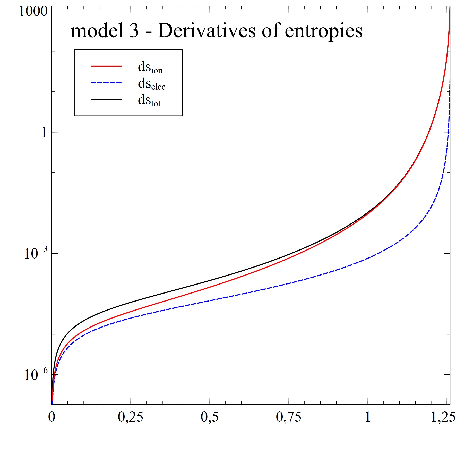
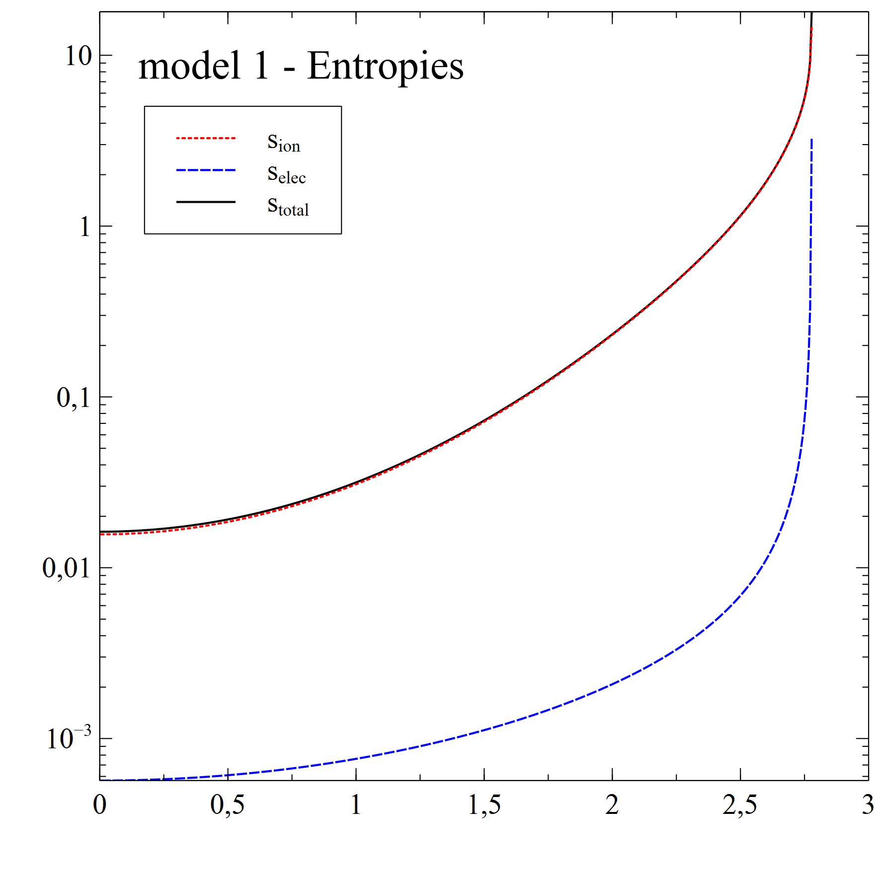
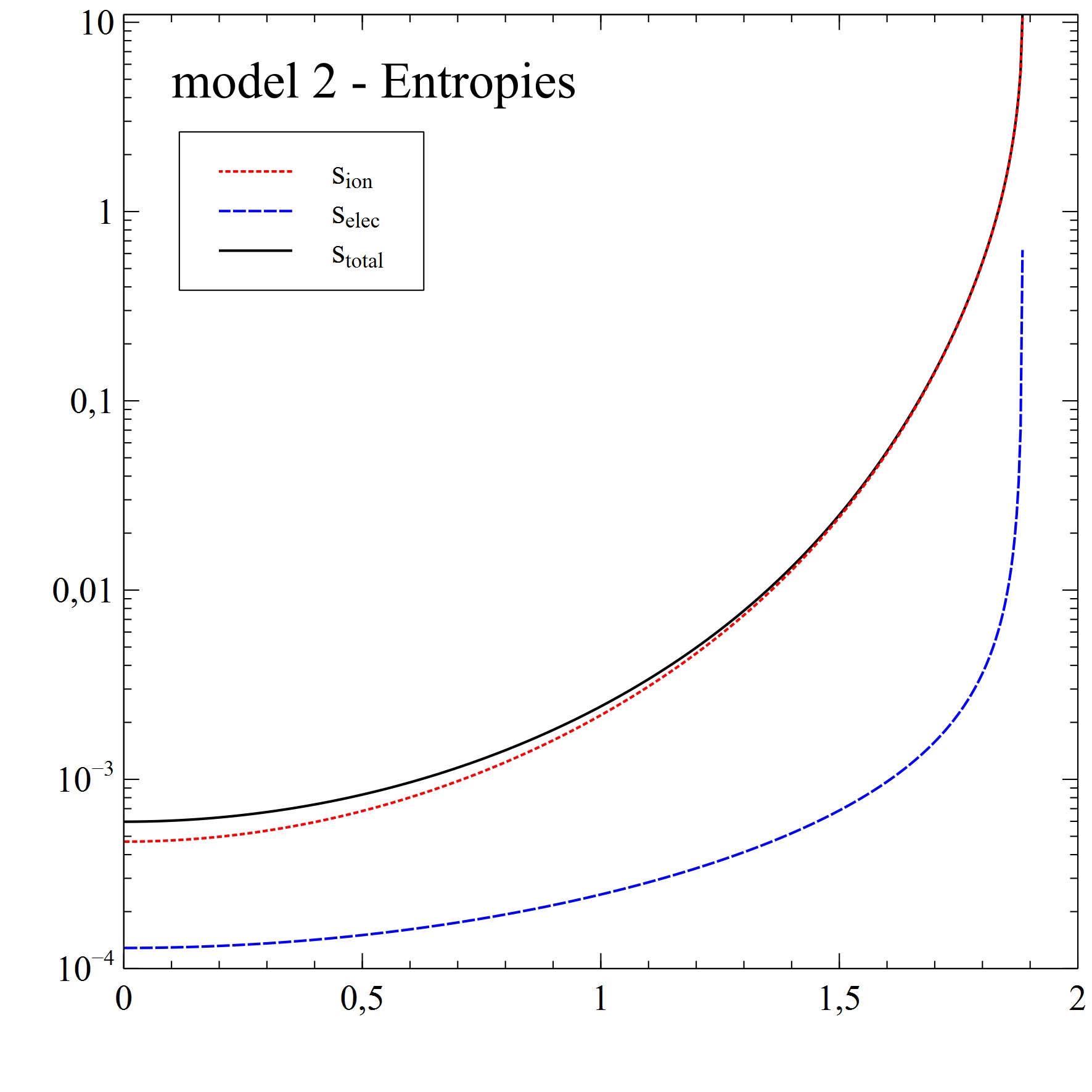
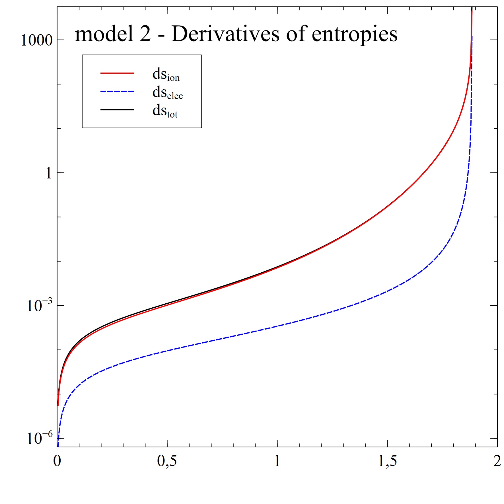
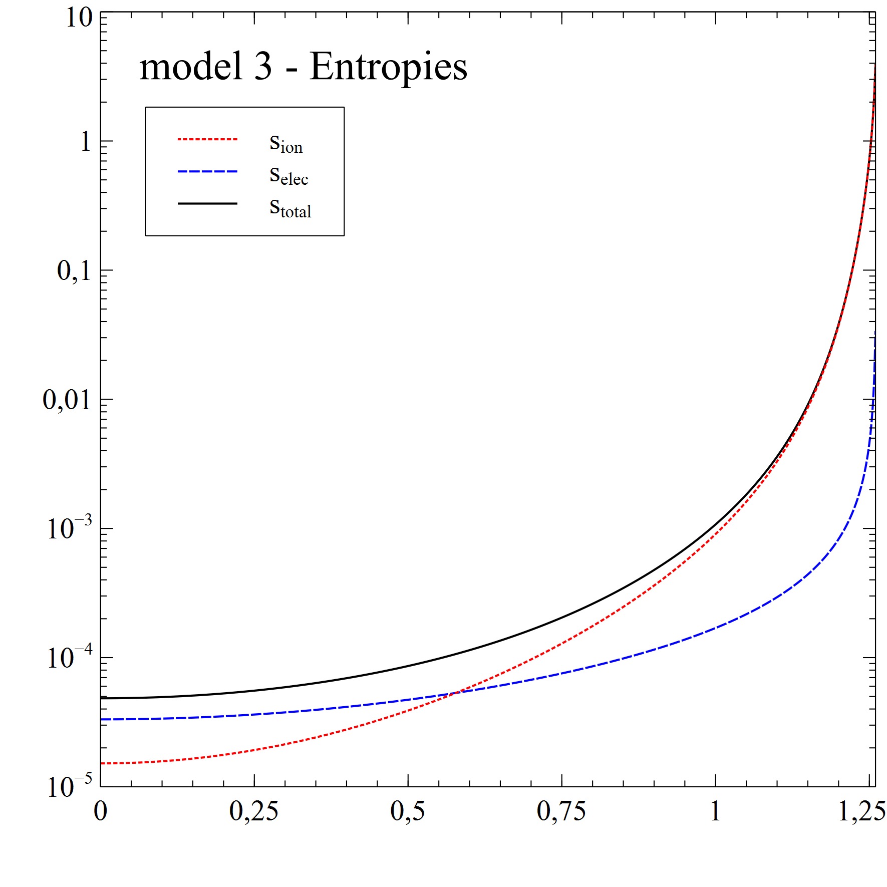
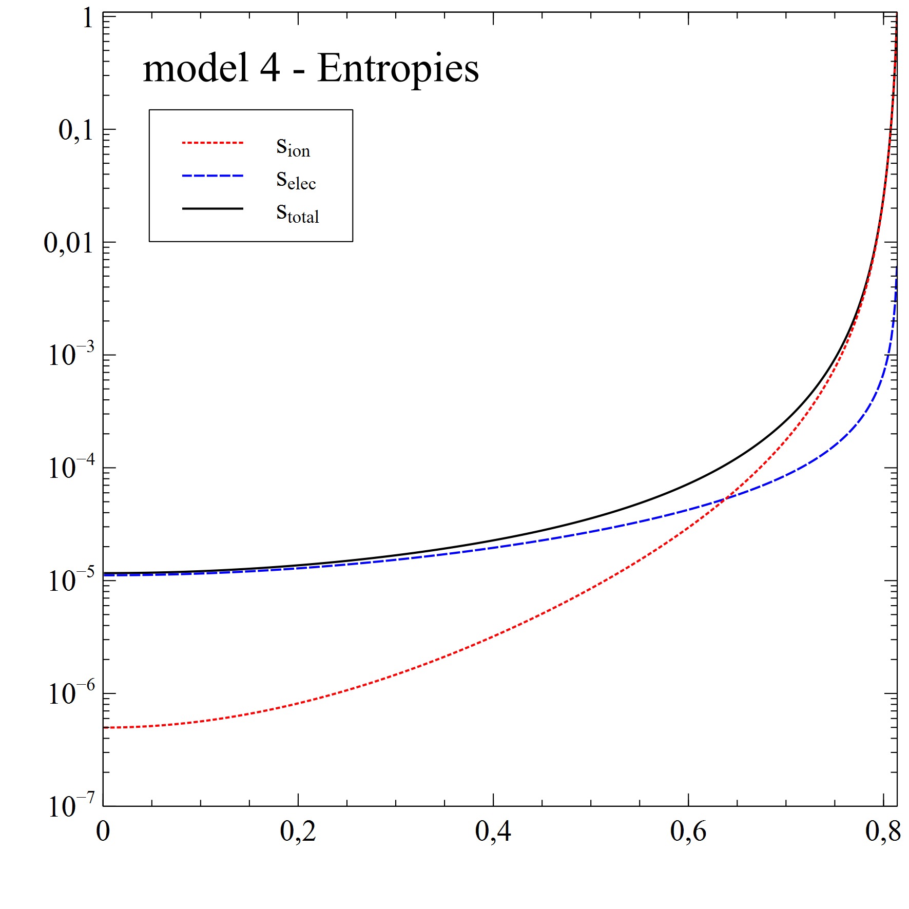
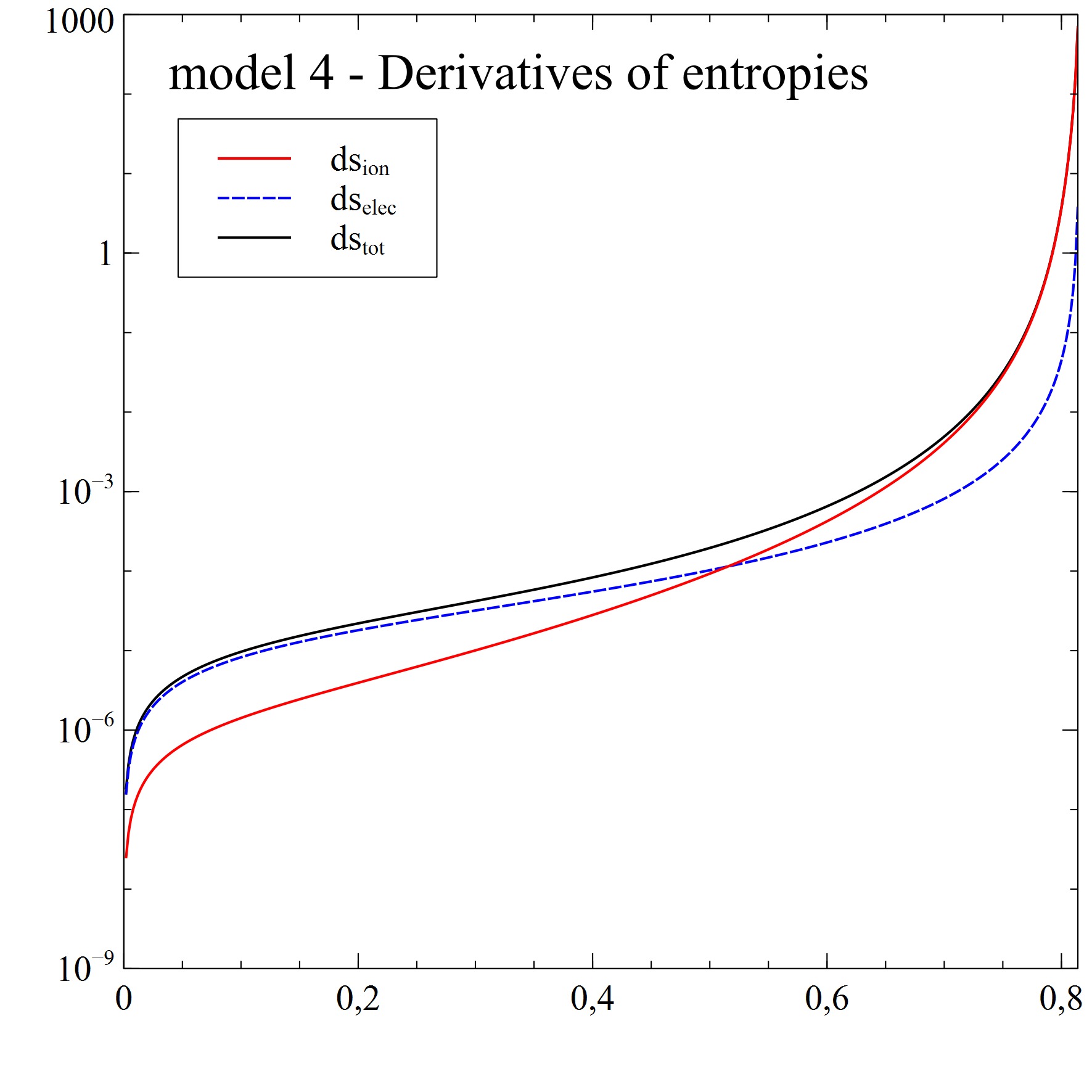
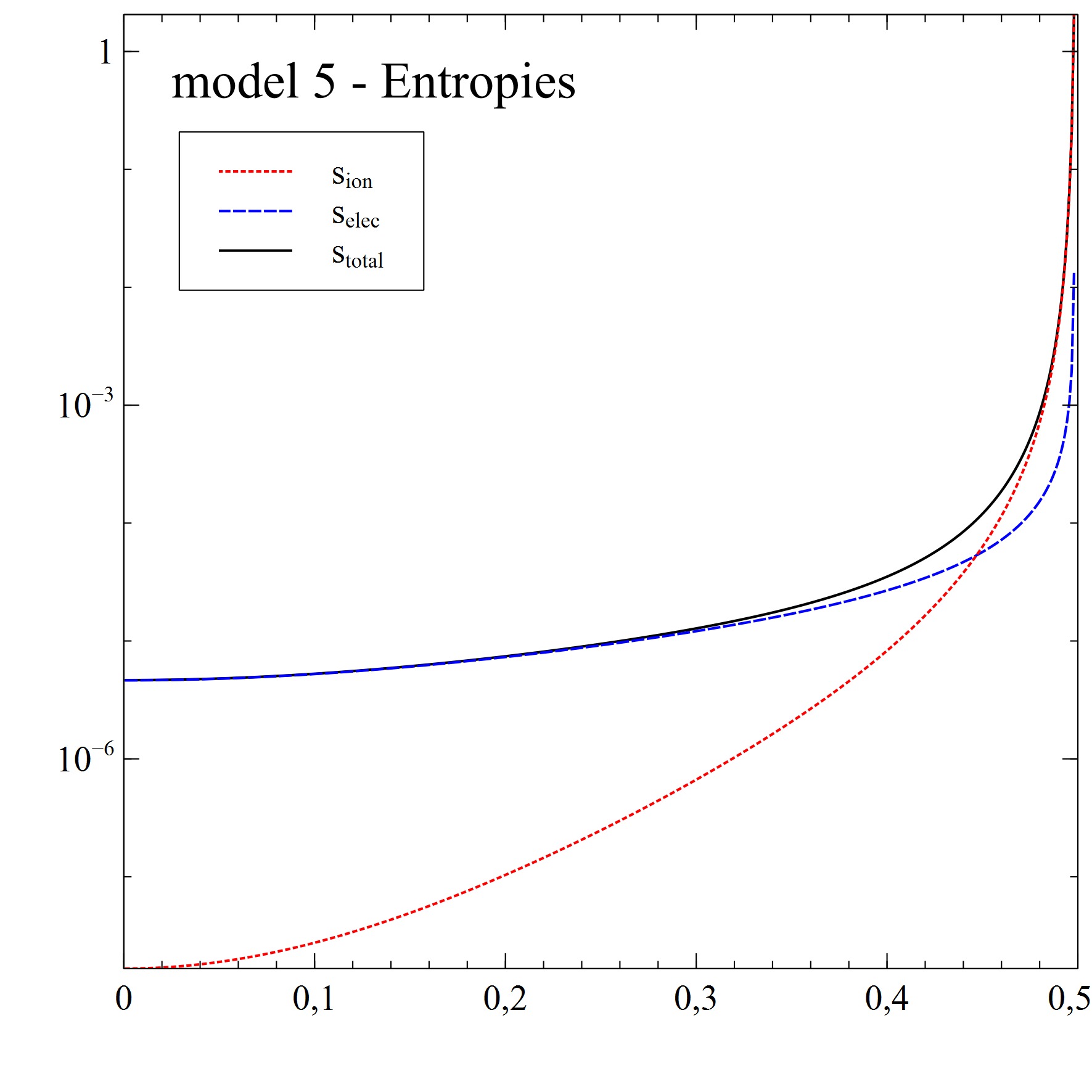
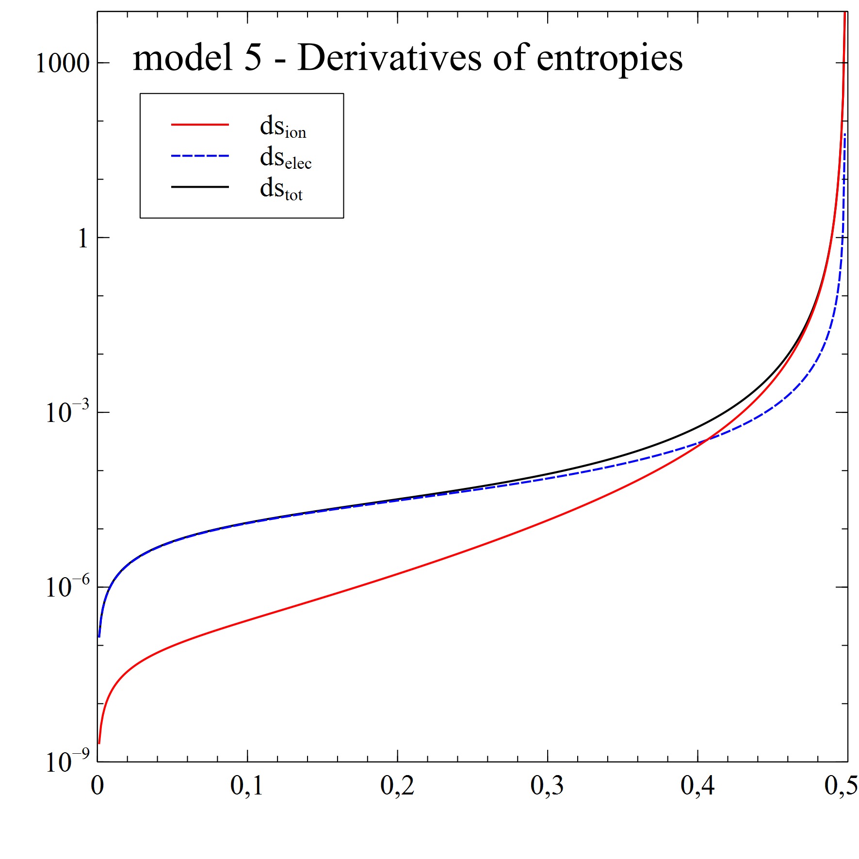
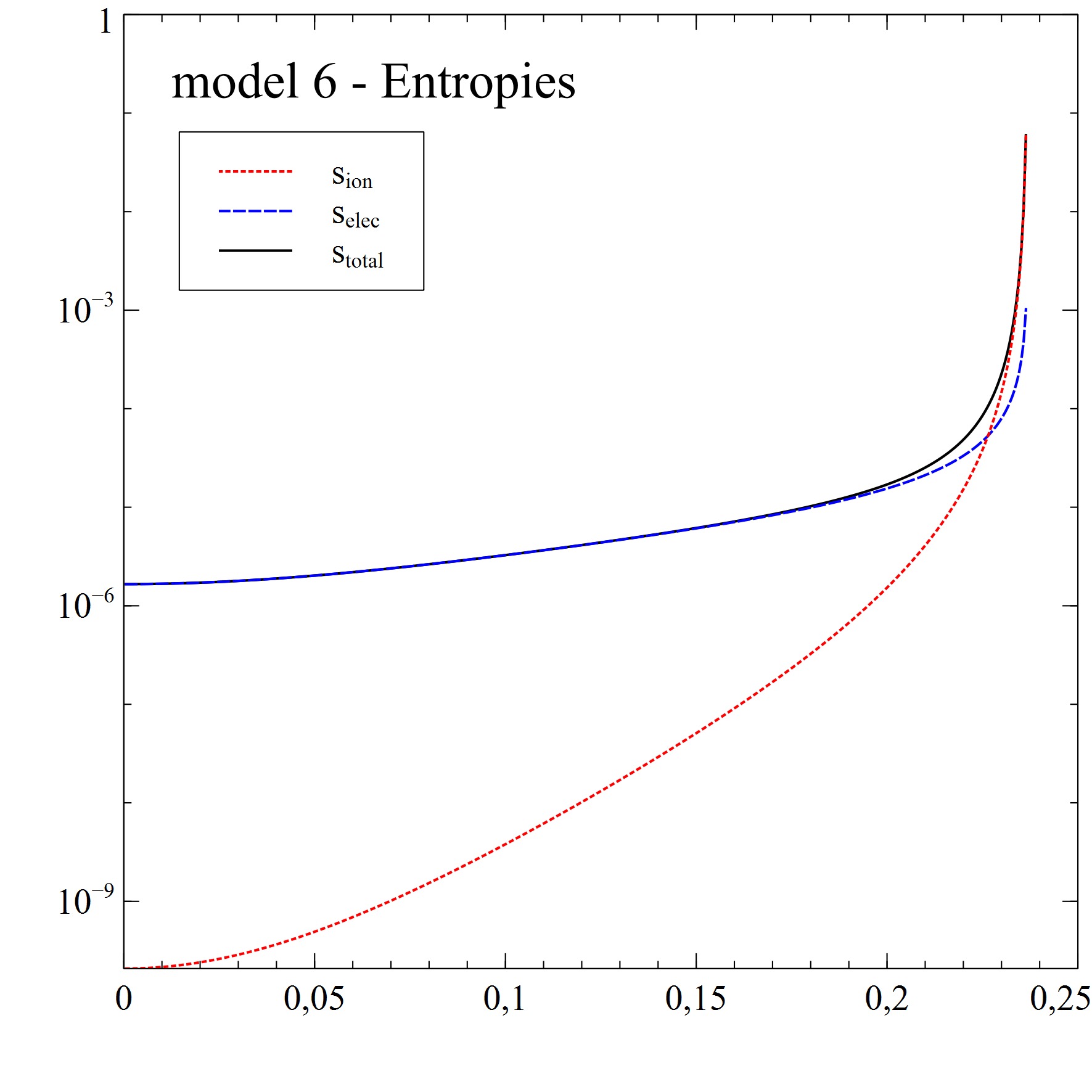
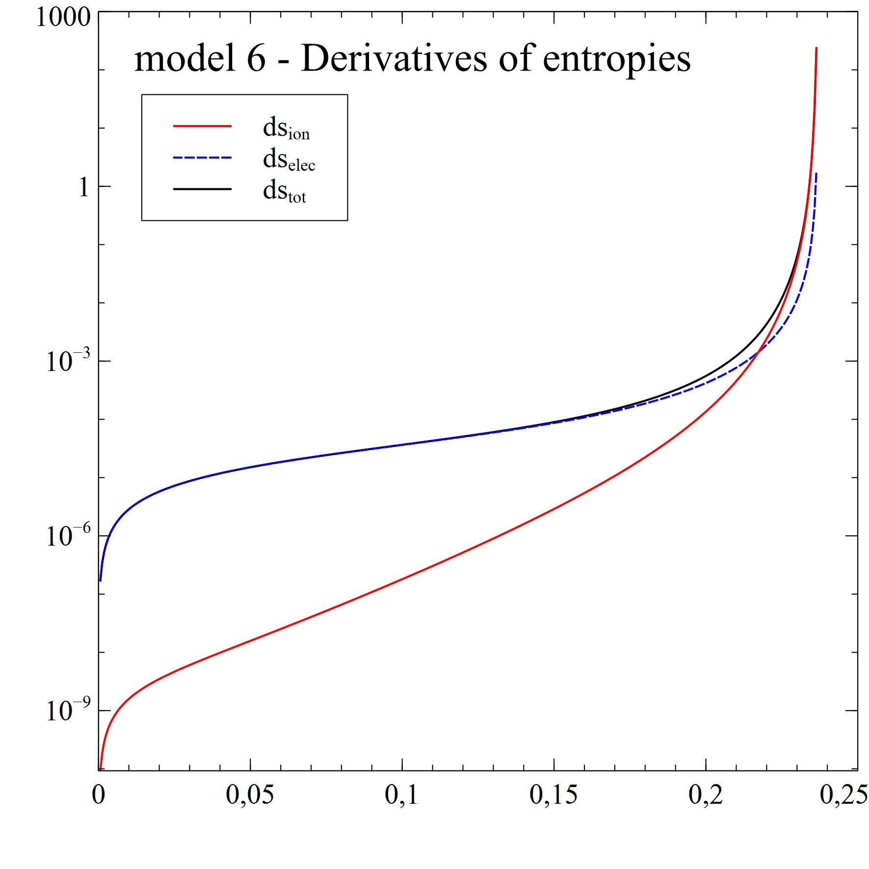
On the horizontal axis we plot the dimensionless radial distance (14), on the vertical axes we enter the dimensional reduced entropy $\hat{s}$ (eq. (32)) in the left plots and $d\hat{s}/d\,x$, i.e., derivatives of reduced entropies in respect to the dimensionless radius $x$ (eq. (14)) in the right plots. As indicated in legends, red dotted curves are ion contributions, blue dashed electron ones and black solid display sums (total values).
Refer to caption Refer to caption
FIG. 3: The same as the previous figure for models 4-6.

For the light WDs (see Fig. 2) the ion entropy prevails, although the electron contribution becomes gradually important, in particular in the inner parts of the WDs. The ion contribution also dominates the energy gradient.

For heavier WDs (see Fig. 3) the electron entropy is more important almost in the whole star, only close to the surface the ion part prevails. The same trend is apparent also for entropy gradient.

As it can be seen from our calculations, the entropy is positivethe positivity of the entropy was noted also in ref. ASJ for all models and the entropy gradient satisfies the condition of the thermodynamical stability of stars Eq.(1.10).

IV Conclusions

The frequently used polytropic model SC1 of the description of the WDs has two drawbacks: a) It is of restricted use, because it is a realistic model of the EoS only in the non-relativistic limit for $\lambda_{c}<<10^{6}g/cm^{3}$ and in the extreme relativistic limit for $\lambda_{c}>>10^{6}g/cm^{3}$.
b) The fluid, described by the polytropic model, is only neutrally stable JPM .
In this paper, we have shown on a representative set of the carbon WDs that their description, based on the EoS formulated in the theory of the magnetized Coulomb plasma in Refs. CP  - ASJ , satisfies the stability requirement, given by eq. (10). As it is seen in Figs. (2) - (7), both the entropy and its gradient are positive.
It would be important to investigate, if this requirement would be satisfied also in the case of the presence of the strong magnetic field. This finding would mean that the existence of strongly magnetized WDs would be possible.

Acknowledgments

One of us (E. T.) thanks Dr. A.Y. Potekhin for the correspondence, discussions and advices. The correspondence with Dr. N. Chamel is acknowledged.

References

  • (1) S. Chandrasekhar, An Introduction to the Study of Stellar Structure, Dover Publications, INC., University Chicago Press, 1939.
  • (2) M. Camenzind, Compact Objects in Astrophysics, Springer Verlag, Berlin, Heidelberg, 2007.
  • (3) A.Y. Potekhin, Phys. Usp.  53 (2010) 1235.
  • (4) S. Chandrasekhar, Astrophys. J.  74 (1931) 81.
  • (5) L.D. Landau, Phys. Z. Sowjetunion  1 (1932) 285.
  • (6) S.L. Shapiro, S.A. Teukolsky, Black Holes, White Dwarfs, and Neutron Stars: The Physics of Compact Objects, Wiley, New York, 1983.
  • (7) J.P. Mitchell, J. Braithwaite, A. Reisenegger, H. Spruit, J.A. Valvidia and N. Langer, Mon. Not. R. Astron. Soc.  447 (2015) 1213.
  • (8) T. Akgün, A. Reisenegger, A. Mastrano and P. Marchant, Mon. Not. R. Astron. Soc.  433 (2013) 2445.
  • (9) J. Braithwaite, Mon. Not. R. Astron. Soc.  397 (2009) 763.
  • (10) H.C. Spruit, Astron. Astrophys.  349 (1999) 189.
  • (11) C.S. Bisnovatyi - Kogan, Stellar Physics 1: Fundamental Concepts and Stellar Equilibrium, Springer, 2001.
  • (12) L. Becerra, A. Reisenegger, J.A. Valvidia and M.E. Gusakov, Mon. Not. R. Astron. Soc.  511 (2022) 732.
  • (13) U. Dass and B. Mukhopadhyay, Int. J. Mod. Phys. D  22 (2013) 134.
  • (14) U. Dass and B. Mukhopadhyay, J. Cosmol. Astropart. Phys.  06 (2014) 050.
  • (15) U. Dass and B. Mukhopadhyay, J. Cosmol. Astropart. Phys.  05 (2015) 016.
  • (16) D. Bera and D. Bhattacharya, Mon. Not. R. Astron. Soc.  465 (2017) 4026.
  • (17) D. Chatterjee, A.F. Fantina, N. Chamel, J. Novak and M. Oertel, Mon. Not. R. Astron. Soc.  469 (2017) 95.
  • (18) N. Chamel, L. Perot, A.F. Fantina, D. Chatterjee, S. Ghosh, J. Novak and M. Oertel, in The 16th Marcel Grossmann Meeting on General Relativity, 5 - 10 July 2021, eds. R. Ruffini and G. Vereshchagin, World Scientific, Singapore, 2023, pp. 4488 - 4507.
  • (19) L. Becerra, K. Boshkayev, J.A. Rueda and R. Ruffini, Mon. Not. R. Astron. Soc.  487 (2019) 812.
  • (20) M. Malheiro, J.A. Rueda and R. Ruffini, Publ. Astron. Soc. Jpn.  64 (2012) 56.
  • (21) N.R. Ikhsanov and N.G. Beskrovnaya, Astron. Rep.  56 (2012) 595.
  • (22) K. Boshkayev, L. Izzo, J.A. Hernandez Rueda and R. Ruffini, Astron. Astrophys.  555 (2013) A151.
  • (23) J.A. Rueda, K. Boshkayev, L. Izzo, R. Ruffini, P. Loren - Aguilar, B. Külebi, G. Aznar - Siguán and E. Garcia - Berro, Astrophys. J.  772 (2013) L24.
  • (24) J.G. Coelho and M. Malheiro, Publ. Astron. Soc. Jpn.  66 (2014) 14.
  • (25) R.V. Lobato, M. Malheiro and J.G. Coelho, Int. J. Mod. Phys. D  25 (2016) 1641025.
  • (26) V.B. Belyaev, P. Ricci, F. Šimkovic, J. Adam, M. Tater and E. Truhlík, Nucl. Phys. A  937 (2015) 17.
  • (27) T.R. Marsh, B.T. Gänsicke, S. Hümmerich et al., Nature  537 (2016) 374.
  • (28) G. Chabrier and A.Y. Potekhin, Phys. Rev. E  58 (1998) 4941.
  • (29) D.A. Baiko, A.Y. Potekhin and D.G. Yakovlev, Phys. Rev. E  64 (2001) 057402.
  • (30) A.Y. Potekhin and G. Chabrier, Phys. Rev. E  62 (2000) 8554.
  • (31) A.Y. Potekhin and G. Chabrier, Contrib. Plasma Phys.  50 (2010) 82.
  • (32) A.Y. Potekhin and G. Chabrier, Astron. Astrophys.  550 (2013) A43.
  • (33) A.S. Jermyn, J. Schwab, E. Bauer, F.X. Timmes and A.Y. Potekhin,
    Astrophys. J.  913 (2021) 72.
  • (34) D.A. Baiko and A.I. Chugunov, Mon. Not. R. Astron. Soc.  510 (2022) 2628.
  • (35) K. Boshkayev, Astron. Rep.  62(12) (2018) 847.
  • (36) N. Chamel and A.F. Fantina, Phys. Rev. D  92 (2015) 023008.
  • (37) C.B. Jackson, J. Taruna, S.L. Pouliot, B.W. Ellison, D.D. Lee, J. Piekarewicz,
    Eur. J. of Phys.  26 (2005) 695 ,arXiv:astro-ph/0409348v2.
  • (38) W.Greiner, L.Neise, H.Stoeker: Thermodynamics and statistical mechanics, Chap. 14, 1995, Springer-Verlag, New York.

Appendix A Scaling And Dimensionless Equations

Let us briefly present an alternative derivation of differential equations describing the WD, starting from the usual Newtonian formulation of the mechanical stability for the spherical WD (which is also a starting point in the main text (2)):

$\displaystyle\frac{d\,P_{e}(r)}{d\,r}$ $\displaystyle=$ $\displaystyle-G\,\frac{M(r)\,\rho(r)}{r^{2}}\ ,$
$\displaystyle\frac{d\,M(r)}{d\,r}$ $\displaystyle=$ $\displaystyle 4\pi\,r^{2}\,\rho(r)\ ,$

where $\rho(r)$ is a matter density:

$\displaystyle\rho(r)$ $\displaystyle=$ $\displaystyle m_{u}\,n_{e}(r),\qquad\mu_{u}\equiv\frac{A}{Z}\,m_{u}\ ,$ (68)

and $P_{e}$ is an electron pressure. In the calculations of this paper we used $A=12,Z=6$ and:

$\displaystyle m_{u}=931.494\,{\rm MeV/c^{2}}\quad\rightarrow\quad\mu_{u}=1\,862.988\,{\rm MeV/c^{2}}\ .$

$M(r)$ is a mass contained inside the radius $r$. It appears convenient to re-write the electron pressure and density in terms of dimensionless quantities $\tilde{P}$ and $\tilde{\rho}$:

$\displaystyle n_{e}$ $\displaystyle=$ $\displaystyle\rho_{0}\,\tilde{n}_{e}\ ,\quad\rho_{0}=\frac{1}{3\pi^{2}\,\lambda^{3}_{e}}\ ,\quad\lambda_{e}=\frac{\hbar}{m_{e}c}\simeq 386.164\,{\rm fm}\ ,$ (69)
$\displaystyle P_{e}$ $\displaystyle=$ $\displaystyle m_{e}c^{2}\,\rho_{0}\,\tilde{P}\ ,$

where $\lambda_{e}$ is the electron Compton length (its value is obtained from $m_{e}\,c^{2}\simeq 0.511\,$MeV and $\hbar\,c\simeq 197.33\,{\rm MeV\cdot fm}$).
The first equation then reads:

$\displaystyle\frac{d\,\tilde{P}(r)}{d\,r}$ $\displaystyle=$ $\displaystyle-G\,\frac{\mu_{u}}{m_{e}c^{2}}\ \frac{M(r)\,\tilde{n}_{e}(r)}{r^{2}}\ .$

Next we re-scale also the radius $r$ (as in (20)) and the mass $M(r)$:

$\displaystyle r=a_{s}\,x\,\qquad M(R)=M_{s}\,\tilde{m}(x)\ .$

In terms of $x$ and $\tilde{m}(x)$ the set of differential equations read:

$\displaystyle\frac{d\,\tilde{P}(x)}{d\,x}$ $\displaystyle=$ $\displaystyle-G\,\frac{\mu_{u}}{m_{e}c^{2}}\,\frac{M_{s}}{a^{2}_{s}}\ \frac{\tilde{m}(x)\,\tilde{n}_{e}(x)}{x^{2}}\ ,$
$\displaystyle\frac{d\,\tilde{m}(x)}{d\,x}$ $\displaystyle=$ $\displaystyle 4\pi\,\mu_{u}\,\rho_{0}\,\frac{a^{3}_{s}}{M_{s}}\ x^{2}\,\tilde{n}_{e}(x)\ .$

The dimensionless constants appearing on the r.h. sides can be fixed to our convenience, we adopt a choice (following ref. JTPELP ):

$\displaystyle G\,\frac{\mu_{u}}{m_{e}c^{2}}\,\frac{M_{s}}{a^{2}_{s}}$ $\displaystyle=$ $\displaystyle\frac{5}{3}\ ,$
$\displaystyle 4\pi\,\mu_{u}\,\rho_{0}\,\frac{a^{3}_{s}}{M_{s}}$ $\displaystyle=$ $\displaystyle 3\ ,$

from which one gets (cp (20))

$\displaystyle a_{s}$ $\displaystyle=$ $\displaystyle\frac{\sqrt{15\pi}}{2\mu_{u}}\,\sqrt{\frac{m_{e}c^{2}\,\lambda_{e}^{3}}{G}}=\frac{\sqrt{15\pi}}{2}\,\lambda_{e}\,\frac{m_{Pl}}{\mu_{u}}\,\simeq 8686.26\,{\rm km}\ ,$ (70)
$\displaystyle M_{s}$ $\displaystyle=$ $\displaystyle a_{s}\cdot\ \frac{5m_{e}c^{2}}{3\mu m_{N}G}\simeq 2.646\,M_{\odot}\ ,$ (71)

where $m_{Pl}$ is the Planck mass (with a corresponding value of the gravitational constant $G$):

$\displaystyle m_{Pl}$ $\displaystyle\equiv$ $\displaystyle\sqrt{\frac{\hbar c}{G}}\simeq 1.2209\cdot 10^{22}\,{\rm MeV}\ ,\quad G\simeq 6.6742\,\cdot 10^{-8}\,{\rm cm^{3}/(g\cdot sec^{2})}\ .$ (72)

The set of the dimensionless DE is now:

$\displaystyle\frac{d\,\tilde{P}(x)}{d\,x}$ $\displaystyle=$ $\displaystyle-\frac{5}{3}\,\frac{\tilde{m}(x)\,\tilde{n}_{e}(x)}{x^{2}}\ ,$
$\displaystyle\frac{d\,\tilde{m}(x)}{d\,x}$ $\displaystyle=$ $\displaystyle 3\,x^{2}\,\tilde{n}_{e}(x)\ .$

To proceed further one has to realize that the quantities $\tilde{P}$ and $\tilde{n}_{e}(x)$ are known functions of a temperature $T$ and electron chemical potential $\mu_{e}$ (taken here without the electron rest mass), or more conveniently, of the dimensionless variables (see the main text):

$\displaystyle\chi_{e}=\mu_{e}\,\beta\ ,\qquad\tau=\frac{1}{\beta\,m_{e}c^{2}}\ ,\qquad\beta=\frac{1}{k_{B}\,T}\ .$

An important simplification then follows from an assumption (employed also in an alternative formulation in the main text) that to a very good approximation the temperature in the WD is constant, i.e. $T$ and hence $\tau$ do not depend on $x$ and are fixed by their initial value. Then all quantities of interest in the WD, in particular $\tilde{P}$ and $\tilde{n}_{e}(x)$, depend on the radius $r$ – and hence on the dimensionless $x$ – implicitly just through a single $x-$dependent function, e.g. $\chi_{e}(x)$. Thus, we can write:

$\displaystyle\frac{d\,\tilde{P}(x)}{d\,x}$ $\displaystyle=$ $\displaystyle\frac{d\,\tilde{P}(x)}{d\,\chi_{e}}\,\frac{d\,\chi_{e}(x)}{d\,x}\ ,$

where the derivative $\tilde{P}(x)/d\,\chi_{e}$ can be calculated from the explicit form of $\tilde{P}=\tilde{P}(\chi_{e},\tau)$. It is convenient to consider instead of $\chi_{e}(x)$ a variable $\varphi(x)$:

$\displaystyle\varphi(x)$ $\displaystyle=$ $\displaystyle\chi_{e}\,\tau=\frac{\mu_{e}}{m_{e}c^{2}}\ ,$

which is a dimensionless electron chemical potential. Its advantage is that for $T=0$ it just reduces to the dimensionless electron Fermi energy $\tilde{\varepsilon}_{F}$:

$\displaystyle\varphi\ \xrightarrow[T\rightarrow 0]{}\ \frac{\tilde{E}_{F}}{m_{e}c^{2}}\equiv\tilde{\varepsilon}_{F}\ ,$ (73)

where $\tilde{E}_{F}$ (and $\tilde{\varepsilon}_{F}$) has a contribution of the electron rest mass subtracted. The resulting set of the DE is then:

$\displaystyle\frac{d\,\varphi(x)}{d\,x}$ $\displaystyle=$ $\displaystyle-\frac{5}{3}\,\frac{\tilde{m}(x)}{x^{2}}\,g(\varphi)\ ,\qquad g(\varphi)=\frac{\tilde{n}_{e}}{\frac{d\,\tilde{P}}{d\,\varphi}}=\frac{\tau\,\tilde{n}_{e}(\chi_{e},\tau)}{\frac{d\,\tilde{P}(\chi_{e},\tau)}{d\,\chi_{e}}}\ ,\qquad\chi_{e}(x)=\frac{\varphi(x)}{\tau}\ ,$ (74)
$\displaystyle\frac{d\,\tilde{m}(x)}{d\,x}$ $\displaystyle=$ $\displaystyle 3\,x^{2}\,\tilde{n}_{e}(x)\ .$ (75)

As for the initial conditions for these equations: $\tilde{m}(0)\equiv\tilde{m}_{c}=0$ (and $\tilde{m}(x)$ is an increasing function of $x$), a value of $\varphi(0)\equiv\varphi_{c}>0$ is related to the central matter density $\lambda_{c}$ and is discussed below ($\varphi(x)$ is a decreasing function of $x$). For the WD the function $g(\varphi)$ is rather close to unity.

The set of DE formulated above has several advantages which we are going to discuss briefly: a) there is a smooth limit of $T\rightarrow 0$. In this limit $\varphi\rightarrow\tilde{\varepsilon}_{F}=\sqrt{1+x^{2}_{r}}-1$, where $x_{r}$ is a dimensionless electron Fermi momentum. Further, for the free electron Fermi gas at $T=0$ it holds:

$\displaystyle\frac{\partial P_{e}}{\partial E_{F}}=n_{e}\ \Rightarrow\ \frac{\partial\tilde{P}}{\varepsilon_{F}}=\tilde{n}_{e}\ \Rightarrow\ g(\varphi)\xrightarrow[T\rightarrow 0]{}1\ \ .$

Thus, our set of coupled DEs for $T\rightarrow 0$ smoothly approaches a set of

$\displaystyle\frac{d\,\tilde{\varepsilon}_{F}(x)}{d\,x}$ $\displaystyle=$ $\displaystyle-\frac{5}{3}\,\frac{\tilde{m}(x)}{x^{2}}\ ,$
$\displaystyle\frac{d\,\tilde{m}(x)}{d\,x}$ $\displaystyle=$ $\displaystyle 3\,x^{2}\,\tilde{n}_{e}(x)=3\,x^{2}\,x^{3}_{r}\ ,$

which is equivalent to DEs considered in JTPELP . This makes comparisons of the finite temperature solutions to $T=0$ ones very transparent.
b) A numerical solution of eqs. (74-75) is straightforward: once one specifies the initial conditions, the equations (complemented by equations for $\tilde{P}(\chi_{e},\tau)$ and $\tilde{n}_{e}(\chi_{e},\tau)$) are solved step by step by appropriate numerical procedure (e.g. 4th order Runge-Kutta) and there is no need to solve numerically at each step some transcendent equation (cp to procedure described in a paragraph following eq. (28)). Moreover, at some point $x_{0}$ the numerical value of the decreasing $\varphi(x)$ crosses zero:

$\displaystyle\varphi(x_{0})=0\ \rightarrow\ r_{0}=a_{s}\,x_{0}\ .$

As in the $T=0$ limit we identify the value of $r_{0}$ with the (dimensionless) radius of the WD. The alternative method used in the main text does not have such a clear criterium for the radius.
c) An initial condition for $\varphi(0)=\varphi_{c}$ is expressed from the central matter density $\lambda_{c}$ (see eq. (14)). Let us express

$\displaystyle\lambda_{c}=\mu_{u}\,\tilde{n}_{c}=\mu_{u}\,x^{3}_{rc}=\mu_{u}\,\tilde{n}_{c}(\chi_{ec},\tau)\ .$ (76)

One can invert this equation numerically to determine $\chi_{ec}$ by a procedure mentioned below eq. (28) (and then to get $\varphi_{c}=\tau\,\chi_{ec}$). Let us emphasize that in this formulation one would have to solve the transcendent equation just once for the central initial value. But even this is actually not necessary. At the center of the WD the density is rather high and $T<<T_{F}$, hence one can use the Sommerfeld expansion, from which it is possible to get an algebraic equation for $\varphi_{c}$ in terms of $\varphi_{0c}=x^{2}_{rc}$ and temperature. We checked that $\varphi_{c}$ obtained this way reproduces very accurately the value obtained by solving eq. (76).

In last part of this appendix we briefly present equations for the WD radius and mass in the Lame-Emden approximation. There are well known textbook equations (see e.g. SLSSAT ) in terms of the central mass density or one can derive very convenient representations for dimensionless radii and masses in terms of the central fractional electron Fermi momentum $x_{rc}$. To crosscheck numbers in our Table 1 we used both versions, so we list below for reference corresponding equations and numerical value.

Recall that the radius $R_{0}$ and the mass of the object described by the Lame-Emden equation (8) are defined by the first zero of its solution $\theta(\xi_{1})=0$ and by its derivative in $f(\xi_{1})=-\xi^{2}_{1}\,\theta^{\prime}(\xi_{1})$

$\displaystyle R_{0}=a\,\xi_{1}$ , $\displaystyle\quad M_{0}=4\pi\,f(\xi_{1})\,a^{3}\,\lambda_{c}$

where according to (9) the LE scaling $a$ is

$\displaystyle a=\sqrt{\frac{n+1}{4\pi}\,\frac{K}{G}\,\lambda_{c}^{\frac{1}{n}-1}}=\sqrt{\tilde{K}}\,\lambda_{c}^{\frac{1-n}{2n}}\ ,\qquad\ .$

For the non-relativistic case with

$$n=\frac{3}{2}\ ,\quad\xi_{1}^{nr}\simeq 3.65375\ ,\quad f(\xi_{1}^{nr})\simeq 2.71406\ ,$$

we get:

$\displaystyle K_{nr}$ $\displaystyle=$ $\displaystyle\frac{\hbar c\,\lambda_{e}}{15\pi^{2}}\,\left(\frac{3\pi^{2}}{\mu_{N}\,m_{u}}\right)^{5/3}\simeq 3.16119\cdot 10^{12}\,\frac{\rm cm^{4}}{\rm g^{2/3}\cdot sec^{2}}\simeq\frac{1.00361\cdot 10^{13}}{\mu_{N}^{5/3}}\,\frac{\rm cm^{4}}{\rm g^{2/3}\cdot sec^{2}}\ ,$

which agrees with eq. (2.3.22) of SLSSAT . Then, introducing

$\displaystyle\tilde{K}_{nr}$ $\displaystyle=$ $\displaystyle\frac{5}{8\pi}\,\frac{K_{nr}}{G}\simeq 9.42283\cdot 10^{18}\,{\rm g^{1/3}\cdot cm}\ ,$

gets (substituting $\lambda_{c}[{\rm g/cm^{3}}]$):

$\displaystyle R_{0}[{\rm km}]$ $\displaystyle=$ $\displaystyle 10^{-5}\cdot\frac{\sqrt{\tilde{K}_{nr}}\,\xi_{1}^{nr}}{\lambda_{c}^{1/6}}\simeq\frac{1.12158\cdot 10^{5}}{\lambda_{c}^{1/6}}=1.12158\cdot 10^{4}\,\left(\frac{\mu_{N}}{2}\right)^{-5/6}\,\left(\frac{\lambda_{c}}{10^{6}}\right)^{-1/6}\ ,$

where the last equation agrees with eq. (3.3.13) of SLSSAT . For the WD mass it follows:

$\displaystyle M$ $\displaystyle=$ $\displaystyle 4\pi\,\tilde{K}_{nr}^{3/2}\,f(\xi^{nr}_{1})\,\sqrt{\lambda_{c}}\simeq 9.86510\cdot 10^{29}\,\sqrt{\lambda_{c}}$
$\displaystyle=$ $\displaystyle 4.95993\cdot 10^{-4}\,M_{\odot}\,\sqrt{\lambda_{c}}=0.495993\,\left(\frac{\mu_{N}}{2}\right)^{-5/2}\,M_{\odot}\,\left(\frac{\lambda_{c}}{10^{6}}\right)^{1/2}\ ,$

where we use $M_{\odot}\simeq 1.98896\cdot 10^{33}\,$g and the result fairy agrees with eq. (3.3.14) of SLSSAT .

Alternatively, we can express from (34) and (35):

$\displaystyle x_{r}\,=\,\frac{\hbar c}{m_{e}c^{2}}\,\bigg{(}\frac{3\pi^{2}\rho}{\mu_{u}}\bigg{)}^{1/3}\,.$ (77)

and express in terms of $x_{r}$ the reduced radius $r_{0}=R_{0}/a_{s}$ and mass $m_{0}=M/m_{S}$, where the scaling factors $a_{s}$ and $M_{s}$ are defined in eqs. (70,71). After some algebra one gets:

$\displaystyle r_{0}$ $\displaystyle=$ $\displaystyle\frac{R_{0}}{R_{s}}=\frac{\xi_{1}^{nr}}{\sqrt{10\,x_{rc}}}\simeq\frac{1.15542}{\sqrt{x_{rc}}}\ ,$ (78)
$\displaystyle m_{0}$ $\displaystyle\equiv$ $\displaystyle\frac{M}{M_{s}}=\frac{3\,f(\xi_{1}^{nr})}{5\,\sqrt{40}}\,x^{3/2}_{rc}\simeq 0.257478\,x^{3/2}_{rc}\ ,$ (79)
$\displaystyle\frac{M}{M_{\odot}}$ $\displaystyle=$ $\displaystyle\frac{M_{s}}{M_{\odot}}\,\cdot m_{0}=\frac{\sqrt{6\pi}}{8}\,f(\xi_{1}^{nr})\,\frac{m^{3}_{\rm pl}}{(\mu_{N}m_{u})^{2}\,M_{\odot}}\,x^{3/2}_{rc}$ (80)
$\displaystyle\simeq$ $\displaystyle 2.68849\,m_{0}\simeq 0.692227\,x^{3/2}_{rc}\ .$

These equations are convenient, since $r_{0}$ and $m_{0}$ depend only on $x_{r}$ and are of natural size. The numbers in the Table 1 were calculated in both ways, yielding identical results.

For the ultra-relativistic case with

$$n=3\ ,\quad\xi_{1}^{ur}\simeq 6.89685\ ,\quad f(\xi_{1}^{ur})\simeq 2.01824\ ,$$

we get:

$\displaystyle K_{ur}$ $\displaystyle=$ $\displaystyle\frac{\hbar c}{12\pi^{2}}\,\left(\frac{3\pi^{2}}{\mu_{u}}\right)^{4/3}\simeq 4.93488\cdot 10^{14}\,\frac{\rm cm^{3}}{\rm g^{1/3}\cdot sec^{2}}\simeq\frac{1.24351\cdot 10^{15}}{\mu_{N}^{4/3}}\,\frac{\rm cm^{3}}{\rm g^{1/3}\cdot sec^{2}}\ ,$

which agrees with eq. (2.3.23) of SLSSAT . We again introduce the auxiliary constant:

$\displaystyle\tilde{K}_{ur}$ $\displaystyle=$ $\displaystyle\frac{K_{ur}}{\pi\,G}\equiv\frac{(3\pi^{2})^{1/3}}{4\pi}\,\frac{m^{2}_{Pl}}{(\mu_{N}\,m_{u})^{4/3}}\simeq 2.35357\,\cdot 10^{21}\,{\rm g^{2/3}}\ .$

Then the radius in km is:

$\displaystyle R_{0}[{\rm km}]$ $\displaystyle=$ $\displaystyle 10^{-5}\cdot\frac{\sqrt{\tilde{K}_{ur}}\,\xi_{1}^{rel}}{\lambda_{c}^{1/3}}\simeq\frac{33.4591}{\lambda_{c}^{1/3}}=0.334591\,\cdot\left(\frac{\mu_{N}}{2}\right)^{-2/3}\,\left(\frac{\lambda_{c}}{10^{6}}\right)^{-1/3}\ ,$

which is consistent with eq. (3.3.16) of SLSSAT . The mass is in the ultra-relativistic limit independent of $\lambda_{c}$ and it is known as the Chandrasekhar limit:

$\displaystyle M$ $\displaystyle=$ $\displaystyle 4\pi\,\tilde{K}_{ur}^{3/2}\,f(\xi^{rel}_{1})\simeq 2.89584\cdot 10^{33}\,{\rm g}\simeq 1.45595\,M_{\odot}=1.45595\,\left(\frac{\mu_{N}}{2}\right)^{-2}\,M_{\odot}\ .$

Alternatively, we can calculate $R_{0}$ and $M/M_{\odot}$ in terms of the dimensionless:

$\displaystyle r_{0}$ $\displaystyle=$ $\displaystyle\frac{\xi_{1}^{rel}}{\sqrt{5}\,x_{rc}}\simeq\frac{3.084370}{x_{rc}}\ ,\quad R_{0}=R_{s}\cdot r_{0}\ ,$ (81)
$\displaystyle m_{0}$ $\displaystyle\equiv$ $\displaystyle\frac{M}{M_{s}}=\frac{3\,f(\xi_{1}^{rel})}{5\,\sqrt{5}}\simeq 0.541550\ ,$ (82)

from which one gets the same result as above:

$\displaystyle\frac{M}{M_{\odot}}$ $\displaystyle=$ $\displaystyle\frac{M_{s}}{M_{\odot}}\,\cdot m_{0}=\frac{\sqrt{3\pi}}{2}\,f(\xi_{1}^{ur})\,\frac{m^{3}_{\rm pl}}{(\mu_{N}m_{u})^{2}\,M_{\odot}}\simeq 1.45595\ .$ (83)

Appendix B Calculations of functions $f_{1}(y)$ and $f_{2}(y)$

In accord with eq. (23) PC3 , the derivative of the electron pressure $P^{(e)}_{id}$ over $y$ is

$$\frac{\partial P^{(e)}_{id}}{\partial y}\,=\,\lambda_{c}\,\frac{\partial P^{(e)}_{id}}{\partial\rho}\,=\,\lambda_{c}\,\frac{n_{\mathrm{e}}}{\rho}\,\bigg{(}\frac{\partial P^{(e)}_{id}}{\partial\chi_{\mathrm{e}}}\bigg{)}_{T}\bigg{/}\bigg{(}\frac{\partial n_{\mathrm{e}}}{\partial\chi_{\mathrm{e}}}\bigg{)}_{T}\,,$$ (84)

and, similarly, the second derivative is

$$\frac{\partial^{2}P^{(e)}_{id}}{\partial y^{2}}\,=\,\lambda_{c}^{2}\,\frac{n_{\mathrm{e}}^{2}}{\rho^{2}}\,\bigg{[}\,\bigg{(}\frac{\partial^{2}P^{(e)}_{id}}{\partial\chi_{\mathrm{e}}^{2}}\bigg{)}\,-\,\bigg{(}\frac{\partial P^{(e)}_{id}}{\partial\chi_{\mathrm{e}}}\bigg{)}\,\bigg{(}\frac{\partial^{2}n_{\mathrm{e}}}{\partial\chi_{\mathrm{e}}^{2}}\bigg{)}\,\bigg{/}\,\bigg{(}\frac{\partial n_{\mathrm{e}}}{\partial\chi_{\mathrm{e}}}\bigg{)}\,\bigg{]}_{T}\,\bigg{/}\bigg{(}\frac{\partial n_{\mathrm{e}}}{\partial\chi_{\mathrm{e}}}\bigg{)}^{2}_{T}\,.$$ (85)

So one should calculate $n_{\mathrm{e}}$ and the derivatives of $P^{(e)}_{id}$ and $n_{\mathrm{e}}$ over $\chi_{\mathrm{e}}$ in terms of the Fermi - Dirac integrals $I_{\nu}(\chi_{\mathrm{e}}\,,\,\tau)$. Identifying

$\displaystyle I_{k+1/2}(\chi_{\mathrm{e}}\,,\,\tau)\,$ $\displaystyle\equiv$ $\displaystyle\,Wk\,,$ (86)
$\displaystyle\frac{\partial I_{k+1/2}(\chi_{\mathrm{e}}\,,\,\tau)}{\partial\chi_{\mathrm{e}}}\,$ $\displaystyle\equiv$ $\displaystyle\,WkDX\,,$ (87)
$\displaystyle\frac{\partial^{2}I_{k+1/2}(\chi_{\mathrm{e}}\,,\,\tau)}{\partial\chi_{\mathrm{e}}^{2}}\,$ $\displaystyle\equiv$ $\displaystyle\,WkDXX\,,$ (88)

one can write the $n_{\mathrm{e}}$ and the derivatives of $P^{(e)}_{id}$ and $n_{\mathrm{e}}$ over $\chi_{\mathrm{e}}$ in terms of $Wk$, $WkDX$ and $WkDXX$ . We calculated these quantities using the program BLIN9 PC3 . We then have

$\displaystyle n_{\mathrm{e}}\,$ $\displaystyle=$ $\displaystyle\,\mathrm{c_{n}}\,[\,W0+\,\tau\,W1\,]\,\equiv\,\mathrm{c_{n}}\,Z_{5}\,,$ (89)
$\displaystyle\frac{\partial n_{\mathrm{e}}}{\partial\chi_{\mathrm{e}}}\,$ $\displaystyle=$ $\displaystyle\,\mathrm{c_{n}}\,[\,W0DX+\,\tau\,W1DX\,]\,\equiv\,\mathrm{c_{n}}\,Z_{3}\,,$ (90)
$\displaystyle\frac{\partial P^{(e)}_{id}}{\partial\chi_{\mathrm{e}}}\,$ $\displaystyle=$ $\displaystyle\,\mathrm{c_{p}}\,[\,W1DX+\,\tau/2\,W2DX\,]\,\equiv\,\mathrm{c_{p}}\,Z_{4}\,,$ (91)
$\displaystyle\frac{\partial^{2}n_{\mathrm{e}}}{\partial\chi_{\mathrm{e}}^{2}}\,$ $\displaystyle=$ $\displaystyle\,\mathrm{c_{n}}\,[\,W0DXX+\,\tau\,W1DXX\,]\,\equiv\,\mathrm{c_{n}}\,Z_{2}\,,$ (92)
$\displaystyle\frac{\partial^{2}P^{(e)}_{id}}{\partial\chi_{\mathrm{e}}^{2}}\,$ $\displaystyle=$ $\displaystyle\,\mathrm{c_{p}}\,[\,W1DXX+\,\tau/2\,W2DXX\,]\,\equiv\,\mathrm{c_{p}}\,Z_{1}\,.$ (93)

In terms of $Z_{i}$ we obtain eq. (84) in the form

$$\frac{\partial P^{(e)}_{id}}{\partial y}\,=\,\frac{\mathrm{c}_{p}}{y}\,\frac{Z_{4}\,Z_{5}}{Z_{3}}\,,$$ (94)

and eq. (85) will be

$$\frac{\partial^{2}P^{(e)}_{id}}{\partial y^{2}}\,=\,\frac{\mathrm{c}_{p}}{y^{2}}\,\frac{Z_{5}^{2}}{Z_{3}^{3}}\,(Z_{1}\,Z_{3}-Z_{2}\,Z_{4})\,,$$ (95)

and finally,

$$f_{1}(y)\,=\,\frac{1}{y}\,\bigg{[}\frac{Z_{5}}{Z_{3}^{2}\,Z_{4}}\,(Z_{1}\,Z_{3}-Z_{2}\,Z_{4})\,-\,1\,\bigg{]}\,,\,\,\,f_{2}(y)\,=\,\frac{\mathrm{c}_{p}}{y}\,\frac{Z_{4}\,Z_{5}}{Z_{3}}\,.$$ (96)

Appendix C The Sommerfeld expansion

In this Appendix we briefly describe how to decompose the thermodynamical quantities for free electrons into series in powers of $k_{\mathrm{B}}T/\tilde{E}_{F}$, where $\tilde{E}_{F}=\mu_{\mathrm{e}}(T=0)$ is the Fermi energy with the rest mass contribution subtracted. We will start from simpler non-relativistic dynamics and later extend the results to a general case.

In the non-relativistic approximation we can write for electron density, momentum and energy density in a conveniently normalized form:

$\displaystyle\left(\frac{n_{\mathrm{e}}(T)}{\rho_{0}}\right)_{nr}$ $\displaystyle=$ $\displaystyle=3\sqrt{2}\,\tau^{3/2}\,I_{1/2}(\chi_{\mathrm{e}})\ ,$ (97)
$\displaystyle\left(\frac{P(T)}{\rho_{0}\,m_{e}c^{2}}\right)_{nr}$ $\displaystyle=$ $\displaystyle 2\sqrt{2}\,\tau^{5/2}\,I_{3/2}\chi_{\mathrm{e}})\ ,$ (98)
$\displaystyle\left(\frac{\tilde{\cal E}(T)}{{\cal E}_{0}}\right)_{nr}$ $\displaystyle=$ $\displaystyle\sqrt{2}\,\tau^{5/2}\,I_{3/2}(\chi_{\mathrm{e}})=\frac{1}{2}\left(\frac{P(T)}{\rho_{0}\,m_{e}c^{2}}\right)_{nr}\ ,\quad{\cal E}_{0}=3\rho_{0}\,m_{e}c^{2}\ ,$ (99)

where the non-relativistic Fermi-Dirac integrals are here defined as:

$\displaystyle I_{\nu}(\chi)=\int\limits_{0}^{\infty}\,\frac{u^{\nu}}{e^{u-\chi}+1}\,du\ ,$ (100)

Substituting into the 1st line of (33) one gets the reduced entropy in the non-relativistic limit:

$\displaystyle s_{e,nr}$ $\displaystyle=$ $\displaystyle\frac{1}{k_{\mathrm{B}}T}\,\left(\frac{5\,m_{e}c^{2}\,\tau\,I_{3/2}(\chi_{\mathrm{e}})}{3\,I_{1/2}(\chi_{\mathrm{e}})}-\mu_{\mathrm{e}}\right)=\frac{5\,I_{3/2}(\chi_{\mathrm{e}})}{3\,I_{1/2}(\chi_{\mathrm{e}})}-\chi_{\mathrm{e}}\ .$

This non-relativistic limit follows also from the general results (33) making use of the relation:

$$I_{\nu}(\chi,\tau)\ \xrightarrow[\tau\rightarrow 0]{}\ I_{\nu}(\chi)\ .$$

An opposite ultra-relativistic limit is obtained from

$\displaystyle I_{\nu}(\chi,\tau)\ \xrightarrow[\tau\rightarrow\infty]{}\ \sqrt{\frac{\tau}{2}}\,I_{\nu+1/2}(\chi)\ .$

The number density, momentum and energy density in the ultra-relativistic limit are:

$\displaystyle\left(\frac{n_{\mathrm{e}}(T)}{\rho_{0}}\right)_{ur}$ $\displaystyle=$ $\displaystyle 3\tau^{3}\,I_{2}(\chi_{\mathrm{e}})\ ,$ (101)
$\displaystyle\left(\frac{P(T)}{\rho_{0}\,m_{e}c^{2}}\right)_{ur}$ $\displaystyle=$ $\displaystyle\left(\frac{\tilde{\cal E}(T)}{{\cal E}_{0}}\right)_{ur}=\tau^{4}\,I_{3}(\chi_{\mathrm{e}})\ .$ (102)

Equations above define the densities of the electron number, pressure and kinetic energy as functions of $\chi_{\mathrm{e}}=\beta\,\mu_{\mathrm{e}}$ and $\tau=k_{\mathrm{B}}T/m_{e}c^{2}$, i.e., functions of the chemical potential $\mu_{\mathrm{e}}$ (not yet determined) and of the temperature $T$ (or of $\beta=k_{\mathrm{B}}T$). According to ref. PC3 the chemical potential $\mu_{\mathrm{e}}(V,T)$ is obtained by (numerically) inverting equation for the density (24) (in its exact or non/ultra-relativistic forms). Assuming the fixed number of electrons $N_{\mathrm{e}}$ (meaning that the electron density $n_{\mathrm{e}}=N_{\mathrm{e}}/V$ explicitly depends only on volume $V$), one gets the chemical potential from the condition $n_{\mathrm{e}}(T)=n_{\mathrm{e}}(0)=N_{\mathrm{e}}/V$, where $n_{\mathrm{e}}(0)$ is known function of the Fermi energy. At the end we get the chemical potential dependent on the temperature $T$ and the Fermi energy, which is its value for zero temperature:

$\displaystyle\mu_{0}$ $\displaystyle\equiv$ $\displaystyle\mu_{\mathrm{e}}(T=0)=\tilde{E}_{F}=m_{e}\,c^{2}\,\tilde{\epsilon}_{F}\ ,$ (103)

where the chemical potential and energies do not include the rest mass contributions.

For a simple non-relativistic case, for which $\mu_{0}=\tilde{E}_{Fnr}/(m_{e}\,c^{2})=\tilde{\epsilon}_{Fnr}=x_{r}^{2}/2$
with $x_{r}=p_{F}/(m_{e}c)$, the l.h.s. of (97) at $T=0$ reads:

$\displaystyle\left(\frac{n_{e}(0)}{\rho_{0}}\right)_{nr}$ $\displaystyle=$ $\displaystyle x^{3}_{r}=\left(2\,\tilde{\epsilon}_{Fnr}\right)^{3/2}=\left(2\,\frac{\mu_{0}}{m_{e}c^{2}}\right)^{3/2}=2\,\sqrt{2}\,\left(\frac{\mu_{0}}{m_{e}c^{2}}\right)^{3/2}\ .$

Equating this to the r.h.s and substituting for $\tau$ yields:

$\displaystyle 2\,\sqrt{2}\,\left(\frac{\mu_{0}}{m_{e}c^{2}}\right)^{3/2}=3\,\sqrt{2}\,\left(\frac{k_{\mathrm{B}}T}{m_{e}c^{2}}\right)^{3/2}\,I_{1/2}(\chi_{\mathrm{e}})\ .$

which simplifies to:

$\displaystyle I_{1/2}(\chi_{\mathrm{e}})=\frac{2}{3}\,\left(\frac{\tilde{\mu}_{0}}{k_{\mathrm{B}}T}\right)^{3/2}=\frac{2}{3}\,\left(\frac{\tilde{E}_{Fnr}}{k_{\mathrm{B}}T}\right)^{3/2}=\frac{2}{3}\,\left(\frac{T_{F}}{T}\right)^{3/2}\ .$ (104)

Denoting by $X_{1/2}$ the inverse function to $I_{1/2}(\chi_{\mathrm{e}})$ one gets a solution for $\chi_{\mathrm{e}}$:

$\displaystyle\chi_{\mathrm{e}}$ $\displaystyle\equiv$ $\displaystyle\frac{\mu}{k_{\mathrm{B}}T}=X_{1/2}\left(\frac{2}{3}\,\left(\frac{T_{F}}{T}\right)^{3/2}\,\right)\ ,$

which is just eq. (17) of ref. CP in our notations. In general, a similar connection is obtained from $n_{e}$ given by (24), in the ultra-relativistic limit from (101).

The relations above are valid for arbitrary temperature, now we will deal with a low temperature expansion. The non-relativistic Fermi-Dirac integrals (100) can be for small temperatures (i.e. large inverse temperatures $\beta=1/k_{B}T$ and hence also $\chi_{\mathrm{e}}=\beta\,\mu_{\mathrm{e}}$) approximated by a power series:

$\displaystyle I_{\nu}(\chi)$ $\displaystyle\simeq$ $\displaystyle\frac{\chi^{\nu+1}}{\nu+1}\,\Big{(}1+\frac{\pi^{2}}{6}\,\frac{(\nu+1)\nu}{\chi^{2}}+\frac{7\,\pi^{4}}{360}\,\frac{(\nu+1)\nu(\nu-1)(\nu-2)}{\chi^{4}}+\dots\Big{)}\ .$ (105)

For the non-relativistic dynamics one needs $I_{\nu}(\chi)$ with $\nu=1/2$ and $\nu=3/2$:

$\displaystyle I_{1/2}(\chi)$ $\displaystyle\simeq$ $\displaystyle\frac{2}{3}\,\chi^{3/2}\,\Big{(}1+\frac{\pi^{2}}{8\,\chi^{2}}+\frac{7\,\pi^{4}}{640\,\chi^{4}}+\dots\Big{)}\ ,$ (106)
$\displaystyle I_{3/2}(\chi)$ $\displaystyle\simeq$ $\displaystyle\frac{2}{5}\,\chi^{5/2}\,\Big{(}1+\frac{5\,\pi^{2}}{8\,\chi^{2}}-\frac{7\,\pi^{4}}{384\,\chi^{4}}+\dots\Big{)}\ .$ (107)

Substituting these relations into (97)-(99) and using $\tau\,\chi_{\mathrm{e}}=\mu_{\mathrm{e}}/(m_{e}c^{2})$ we get:

$\displaystyle\frac{1}{3\sqrt{2}}\left(\frac{n_{\mathrm{e}}(T)}{\rho_{0}}\right)_{nr}$ $\displaystyle=$ $\displaystyle\tau^{3/2}\,I_{1/2}(\chi_{\mathrm{e}})\simeq\frac{2}{3}\left(\frac{\mu_{\mathrm{e}}}{m_{e}c^{2}}\right)^{3/2}\,\left(1+\frac{\pi^{2}}{8\chi_{\mathrm{e}}^{2}}+\frac{7\pi^{4}}{640\chi_{\mathrm{e}}^{4}}+\dots\right)\ ,$ (108)
$\displaystyle\frac{1}{2^{3/2}}\left(\frac{P(T)}{\rho_{0}\,m_{e}c^{2}}\right)_{nr}$ $\displaystyle=$ $\displaystyle\frac{1}{\sqrt{2}}\left(\frac{\tilde{\cal E}(T)}{{\cal E}_{0}}\right)_{nr}=\tau^{5/2}\,I_{3/2}(\chi_{\mathrm{e}})$ (109)
$\displaystyle\simeq$ $\displaystyle\frac{2}{5}\left(\frac{\mu_{\mathrm{e}}}{m_{e}c^{2}}\right)^{5/2}\,\left(1+\frac{5\pi^{2}}{8\chi_{\mathrm{e}}^{2}}-\frac{7\pi^{4}}{384\chi_{\mathrm{e}}^{4}}+\dots\right)\ .$

These are formal power series in terms of powers of the so far unknown $1/\chi_{\mathrm{e}}^{2}\,$. Recall that $\chi_{\mathrm{e}}$ depends on temperature and on the chemical potential. As discussed above, $\mu_{\mathrm{e}}$ is determined from the condition $n_{\mathrm{e}}(T)=n_{\mathrm{e}}(0)$ (but now with $n_{\mathrm{e}}(T)$ decomposed into the power series above). Substituting $1/\chi_{\mathrm{e}}^{2}=(kT)^{2}/\mu_{\mathrm{e}}^{2}$ (and using $\mu_{0}=\tilde{E}_{Fnr}$ for the non-relativistic Fermi energy) leads to:

$\displaystyle\mu_{0}$ $\displaystyle=$ $\displaystyle\mu_{\mathrm{e}}\,\left(1+\frac{1}{8}\frac{(\pi k_{\mathrm{B}}T)^{2}}{\mu_{\mathrm{e}}^{2}}+\frac{7}{640}\frac{(\pi k_{\mathrm{B}}T)^{4}}{\mu_{\mathrm{e}}^{4}}+\dots\right)^{2/3}\ .$ (110)

This relation can be perturbatively inverted by assuming the power series for $\mu_{\mathrm{e}}$ (in powers of $(k_{\mathrm{B}}T/\mu_{0})^{2}$):

$\displaystyle\mu_{\mathrm{e}}$ $\displaystyle=$ $\displaystyle\mu_{0}\,\left(1-\frac{\pi^{2}}{12}\frac{(k_{\mathrm{B}}T)^{2}}{\mu_{0}^{2}}-\frac{\pi^{4}}{80}\frac{(k_{\mathrm{B}}T)^{4}}{\mu_{0}^{4}}+\dots\right)\ .$ (111)

Substituting (111) into the r.h.s. of and (109) and making the Taylor decomposition in powers of $(k_{\mathrm{B}}T)^{2}$ yields the following non-relativistic equations for the observables:

$\displaystyle P_{nr}(T)$ $\displaystyle=$ $\displaystyle m_{e}c^{2}\,\rho_{0}\ \frac{x^{5}_{r}}{5}\,\left(1+\frac{5\pi^{2}}{12}\frac{(k_{\mathrm{B}}T)^{2}}{\mu^{2}_{0}}-\frac{\pi^{4}}{16}\frac{(k_{\mathrm{B}}T)^{4}}{\mu^{4}_{0}}+\dots\right)\ ,$ (112)
$\displaystyle\tilde{\cal E}_{nr}(T)$ $\displaystyle=$ $\displaystyle\frac{3}{2}\,P_{nr}(T)\ .$ (113)

These results are consistent with the equations, presented in (Grei ) (where slightly different notation is used).

For the ultra-relativistic dynamics one proceeds in a similar way. For sake of briefness, we cite just the final results (using $\mu_{0}/(m_{e}c^{2})=\epsilon_{Fur}=x_{r}$):

$\displaystyle\mu_{\mathrm{e}}$ $\displaystyle=$ $\displaystyle\mu_{0}\,\left(1-\frac{\pi^{2}}{3}\frac{(kT)^{2}}{\mu_{0}^{2}}+O(T^{6})\right)\ .$ (114)
$\displaystyle n_{e,ur}(T)$ $\displaystyle=$ $\displaystyle n_{e,ur}(0)=\rho_{0}\,\left(\frac{\mu_{0}}{m_{e}c^{2}}\right)^{3}=\rho_{0}\,\epsilon^{3}_{Fur}=\rho_{0}\,x_{r}^{3}=\frac{N_{e}}{V}\ ,$ (115)
$\displaystyle P_{ur}(T)$ $\displaystyle=$ $\displaystyle\rho_{0}\,m_{e}c^{2}\,\frac{x^{4}_{r}}{4}\,\left(1+\frac{2\pi^{2}}{3}\frac{(k_{\mathrm{B}}T)^{2}}{\mu^{2}_{0}}-\frac{\pi^{4}}{5}\frac{(k_{\mathrm{B}}T)^{4}}{\mu^{4}_{0}}+\dots\right)\ ,$ (116)
$\displaystyle\tilde{\cal E}_{ur}(T)$ $\displaystyle=$ $\displaystyle 3\,P_{ur}(T)\ .$ (117)

When the non-relativistic or ultra-relativistic limits cannot be applied, we start from normalized equations (24-26):

$\displaystyle\frac{n_{\mathrm{e}}(T)}{\rho_{0}}$ $\displaystyle=$ $\displaystyle 3\sqrt{2}\,\tau^{3/2}\,\left[I_{1/2}(\chi_{\mathrm{e}},\tau)+\tau\,I_{3/2}(\chi_{\mathrm{e}},\tau)\right]\ ,\quad\rho_{0}=\frac{1}{3\pi^{2}\,\lambda^{3}_{e}}\ ,$ (118)
$\displaystyle\frac{P(T)}{\rho_{0}\,m_{e}c^{2}}$ $\displaystyle=$ $\displaystyle 2\sqrt{2}\,\tau^{5/2}\,\left[I_{3/2}(\chi_{\mathrm{e}},\tau)+\frac{\tau}{2}\,I_{5/2}(\chi_{\mathrm{e}},\tau)\right]\ ,$ (119)
$\displaystyle\frac{\tilde{\cal E}(T)}{{\cal E}_{0}}$ $\displaystyle=$ $\displaystyle\sqrt{2}\,\tau^{5/2}\,\left[I_{3/2}(\chi_{\mathrm{e}},\tau)+\tau\,I_{5/2}(\chi_{\mathrm{e}},\tau)\right]\ ,\quad{\cal E}_{0}=3\rho_{0}\,m_{e}c^{2}\ .$ (120)

Now, we will need the following Sommerfeld decompositions of the generalized Fermi-Dirac integrals (denoting $\varphi=\tau\,\chi=\mu_{\mathrm{e}}/(m_{e}c^{2})$):

$\displaystyle I_{1/2}(\chi,\tau)$ $\displaystyle\simeq$ $\displaystyle\frac{1}{\sqrt{2}\,\tau^{3/2}}\,\left\{\frac{1}{2}\,\left[(1+\varphi)\sqrt{\varphi(2+\varphi)}-{\rm ln}\left(1+\varphi+\sqrt{\varphi(2+\varphi)}\right)\,\right]+\right.$ (121)
$\displaystyle\hskip 56.9055pt\left.+\frac{(1+\varphi)}{\sqrt{\varphi(2+\varphi)}}\,\frac{\pi^{2}\tau^{2}}{6}+\frac{(1+\varphi)}{[\varphi(2+\varphi)]^{5/2}}\,\frac{7\pi^{4}\tau^{4}}{120}+\dots\right\}\ ,$
$\displaystyle I_{3/2}(\chi,\tau)$ $\displaystyle\simeq$ $\displaystyle\frac{1}{\sqrt{2}\,\tau^{5/2}}\,\left\{\frac{2\varphi^{2}+\varphi-3}{6}\,\sqrt{\varphi(2+\varphi)}+\frac{1}{2}{\rm ln}\left(1+\varphi+\sqrt{\varphi(2+\varphi)}\right)\right.$ (122)
$\displaystyle\hskip 56.9055pt\left.+\frac{\sqrt{\varphi}\,(3+2\varphi)}{\sqrt{2+\varphi}}\,\frac{\pi^{2}\tau^{2}}{6}-\frac{1}{\varphi^{3/2}\,(2+\varphi)^{5/2}}\,\frac{7\pi^{4}\tau^{4}}{120}+\dots\right\}\ ,$
$\displaystyle I_{5/2}(\chi,\tau)$ $\displaystyle\simeq$ $\displaystyle\frac{1}{\sqrt{2}\,\tau^{7/2}}\,\left\{\frac{(6\varphi^{3}+2\varphi^{2}-5\varphi+15)\sqrt{\varphi(2+\varphi)}}{24}\,-\frac{5}{8}{\rm ln}\left(1+\varphi+\sqrt{\varphi(2+\varphi)}\right)\right.$ (123)
$\displaystyle\hskip 14.22636pt\left.+\frac{\varphi^{2}\,(3\varphi+5)}{\sqrt{\varphi(2+\varphi)}}\,\frac{\pi^{2}\tau^{2}}{6}+\frac{\varphi^{2}(2\varphi^{3}+10\varphi^{2}+15\varphi+5)}{[\varphi(2+\varphi)]^{5/2}}\,\frac{7\pi^{4}\tau^{4}}{120}+\dots\right\}\ .$

Now we again first find the chemical potential from the condition $n_{\mathrm{e}}(T)=n_{\mathrm{e}}(0)$. Substituting (121,122) into equation (118) for $n_{\mathrm{e}}(T)$ yields (the logarithmic terms are cancel each other):

$\displaystyle\frac{n_{\mathrm{e}}(T)}{\rho_{0}}\simeq\left[\varphi(2+\varphi)\right]^{3/2}+\frac{(2\varphi^{2}+4\varphi+1)}{\sqrt{\varphi(2+\varphi)}}\,\frac{\pi^{2}\tau^{2}}{2}+\frac{1}{[\varphi(2+\varphi)]^{5/2}}\,\frac{7\pi^{4}\tau^{4}}{40}+\dots\ .$ (124)

For $T=0$ it holds $\tau=0$ and

$\displaystyle\varphi(0)\equiv\varphi_{0}=\frac{\mu_{0}}{m_{e}c^{2}}=\tilde{\epsilon}_{F}=\epsilon_{F}-1\ ,\quad\epsilon_{F}=\sqrt{1+x^{2}_{r}}\ .$

This relation implies:

$\displaystyle\varphi_{0}(2+\varphi_{0})=(\epsilon_{F}-1)(\epsilon_{F}+1)=\epsilon_{F}^{2}-1=x^{2}_{r}\ ,$

which reproduces the electron density at zero temperature: from the relation (124) one gets

$\displaystyle n_{\mathrm{e}}(0)$ $\displaystyle=$ $\displaystyle\rho_{0}\,\left[\varphi_{0}(2+\varphi_{0})\right]^{3/2}=\rho_{0}\,x^{3}_{r}\equiv\rho_{F}\ .$

Using (124) one gets from $n_{\mathrm{e}}(0)=n_{\mathrm{e}}(T)$ an implicit relation between $\varphi_{0}$ and $\varphi$:

$\displaystyle\varphi_{0}(2+\varphi_{0})=\varphi(2+\varphi)\,\left[1+\frac{(2\varphi^{2}+4\varphi+1)\,B}{2[\varphi(2+\varphi)]^{2}}+\frac{7\,B^{2}}{40[\varphi(2+\varphi)]^{4}}+\dots\right]^{2/3}\ ,$ (125)

where $B=\pi^{2}\,\tau^{2}$. To solve this constraint we assume for $\varphi=\mu_{\mathrm{e}}/(m_{e}c^{2})$ a perturbative expansion in a form:

$\displaystyle\varphi$ $\displaystyle=$ $\displaystyle\varphi_{0}\,\left(1+c_{1}\frac{B}{\varphi^{2}_{0}}+c_{2}\frac{B^{2}}{\varphi^{4}_{0}}+\dots\right)\ .$ (126)

Notice that:

$\displaystyle\frac{B}{\varphi^{2}_{0}}$ $\displaystyle=$ $\displaystyle\frac{\pi^{2}(k_{\mathrm{B}}T)^{2}}{(m_{e}c^{2})^{2}}\,\frac{(m_{e}c^{2})^{2}}{\mu_{0}^{2}}=\frac{\pi^{2}(k_{\mathrm{B}}T)^{2}}{\mu_{0}^{2}}\ ,$

hence our Ansatz for $\varphi$ above is identical to the Ansatz used for $\mu_{\mathrm{e}}$ in previous sections. Substituting (126) into (125), making the Taylor decomposition in powers of $B$ and requiring that the coefficients in front of $B^{n},n\geq 1$ are equal to zero, yields the coefficients $c_{i}$ in terms of $\varphi_{0}$. The first two are given by relatively simple equations:

$\displaystyle c_{1}$ $\displaystyle=$ $\displaystyle-\frac{2\varphi^{2}_{0}+4\varphi_{0}+1}{6(\varphi^{2}_{0}+3\varphi_{0}+2)}=-\frac{2\epsilon^{2}_{F}-1}{6\epsilon_{F}(\epsilon_{F}+1)}\ ,$ (127)
$\displaystyle c_{2}$ $\displaystyle=$ $\displaystyle-\frac{20\varphi^{4}_{0}+80\varphi^{3}_{0}+141\varphi^{2}_{0}+122\varphi_{0}+36}{360(\varphi^{2}_{0}+3\varphi_{0}+2)^{3}}=-\frac{20\epsilon^{4}_{F}+21\epsilon^{2}_{F}-5}{360\epsilon^{3}_{F}(\epsilon_{F}+1)^{3}}\ .$ (128)

With these $c_{1}$ and $c_{2}$ in (126) the Taylor decomposition of (125) has a first non-zero coefficients (apart from the constant $\varphi_{0}(2+\varphi_{0})$ term) in front of the power $B^{3}$.

Let us now derive the perturbative series for the pressure and the kinetic energy. Substituting the decompositions of $I_{3/2}(\chi_{\mathrm{e}},\tau)$ (see 122) and $I_{5/2}(\chi_{\mathrm{e}},\tau)$ (see 123) into (119) and (120) yields:

$\displaystyle\frac{P(T)}{\rho_{0}\,m_{e}c^{2}}$ $\displaystyle=$ $\displaystyle\frac{(2\varphi^{3}+6\varphi^{2}+\varphi-3)\sqrt{\varphi(2+\varphi)}}{8}+\frac{3}{8}\,{\rm ln}\left(1+\varphi+\sqrt{\varphi(2+\varphi)}\right)$
$\displaystyle+\frac{(\varphi^{3}+3\varphi^{2}+2\varphi)}{\sqrt{\varphi(2+\varphi)}}\,\frac{\pi^{2}\theta^{2}}{2}+\frac{(2\varphi^{5}+10\varphi^{4}+15\varphi^{3}+5\varphi^{2}-2\varphi)}{[\varphi(2+\varphi)]^{5/2}}\,\frac{7\pi^{4}\theta^{4}}{120}+\dots\ ,$
$\displaystyle\frac{\tilde{\cal E}(T)}{{\cal E}_{0}}$ $\displaystyle=$ $\displaystyle\frac{(6\varphi^{3}+10\varphi^{2}-\varphi+3)\sqrt{\varphi(2+\varphi)}}{24}-\frac{1}{8}\,{\rm ln}\left(1+\varphi+\sqrt{\varphi(2+\varphi)}\right)$
$\displaystyle+\frac{(3\varphi^{3}+7\varphi^{2}+3\varphi)}{\sqrt{\varphi(2+\varphi)}}\,\frac{\pi^{2}\theta^{2}}{6}+\frac{(2\varphi^{5}+10\varphi^{4}+15\varphi^{3}+5\varphi^{2}-\varphi)}{[\varphi(2+\varphi)]^{5/2}}\,\frac{7\pi^{4}\theta^{4}}{120}+\dots\ .$

What remains is to substitute $\varphi$ expressed in terms of $\varphi_{0}$ and powers of $B$ (see eqs. (126)-(128)) into equations for the pressure (C) and kinetic energy (C) and decompose into the Taylor series in powers of $B$. This is not so simple as for the limiting non-relativistic and ultra-relativistic cases considered above, since the coefficients depend on $\varphi_{0}$ and also $P(0)$ and ${\cal E}(0)$ are now not just simple powers of $\varphi_{0}$ and cannot be simply factorized. Nevertheless, with the help of Mathematica the power decomposition can be performed. We made a decomposition up to the order $B^{2}$, but the terms $\sim B^{2}$ are is lengthy and clumsy. hence, we for the sake of briefness present just leading and next-to-leading orders:

$\displaystyle\frac{P(T)}{\rho_{0}\,m_{e}c^{2}}$ $\displaystyle=$ $\displaystyle\frac{P(0)}{\rho_{0}\,m_{e}c^{2}}+\frac{\varphi_{0}(2+\varphi_{0})(\varphi_{0}^{2}+2\varphi_{0}+2)\,B}{6(1+\varphi_{0})\sqrt{\varphi_{0}(2+\varphi_{0})}}$ (131)
$\displaystyle=$ $\displaystyle\frac{P(0)}{\rho_{0}\,m_{e}c^{2}}+\frac{x_{r}(\epsilon_{F}^{2}+1)}{6\epsilon_{F}}\,B\ ,\quad B=\pi^{2}\,\tau^{2}\ ,$
$\displaystyle\frac{\tilde{\cal E}(T)}{{\cal E}_{0}}$ $\displaystyle=$ $\displaystyle\frac{\tilde{\cal E}(0)}{{\cal E}_{0}}+\frac{\varphi_{0}(2+\varphi_{0})(1+\varphi_{0})\,B}{6\sqrt{\varphi_{0}(2+\varphi_{0})}}=\frac{\tilde{\cal E}(0)}{{\cal E}_{0}}+\frac{x_{r}\,\epsilon_{F}}{6}\,B\ .$ (132)

C.1 Sommerfeld decomposition of entropy

Recall the equation for the dimensionless reduced entropy of free electrons (33):

$\displaystyle\hat{s}_{e}$ $\displaystyle\equiv$ $\displaystyle\frac{1}{k_{B}}\,\frac{S_{e}}{N_{e}}\equiv\frac{1}{k_{B}\,T}\,\Sigma\ ,\quad\Sigma=\frac{\tilde{\cal E}+P_{e}}{n_{e}}-\mu_{\mathrm{e}}\ ,$ (133)

where it is convenient to separate for a while a factor $\Sigma$. We re-write this factor in a convenient form:

$\displaystyle\Sigma$ $\displaystyle=$ $\displaystyle\frac{\tilde{\cal E}+P_{e}}{n_{e}}-\mu_{\mathrm{e}}=\left[\frac{\tilde{\cal E}(0)+P_{e}(0)}{n_{e}}-\mu_{\mathrm{e}}\right]+\frac{\Delta\tilde{\cal E}+\Delta P_{e}}{n_{e}}=\Sigma_{1}+\Sigma_{2}\ ,$ (134)

where $\Delta\tilde{\cal E}=\tilde{\cal E}(T)-\tilde{\cal E}(0)$ and $\Delta P_{e}=P_{e}(T)-P_{e}(0)$. From relations (C,C) at $T=0$ and from $\varphi(0)\equiv\varphi_{0}=\tilde{\epsilon}_{F}$ one gets:

$\displaystyle\tilde{\cal E}(0)+P_{e}(0)$ $\displaystyle=$ $\displaystyle m_{e}c^{2}\,\rho_{0}\,x^{3}_{r}\,\tilde{\epsilon}_{F}=m_{e}c^{2}\,n_{e}\,\tilde{\epsilon}_{F}\ \rightarrow\ \frac{\tilde{\cal E}(0)+P_{e}(0)}{n_{e}}=m_{e}c^{2}\,\varphi_{0}\ .$

Making use of $\mu_{\mathrm{e}}=m_{e}c^{2}\,\varphi$ we write the first term of $\Sigma$ in a compact form:

$\displaystyle\Sigma_{1}$ $\displaystyle=$ $\displaystyle\frac{\tilde{\cal E}(0)+P_{e}(0)}{n_{e}}-\mu_{\mathrm{e}}=-m_{e}\,c^{2}\,(\varphi-\varphi_{0})\ .$ (135)

The low temperature decomposition of this equation follows from (126):

$\displaystyle\varphi-\varphi_{0}$ $\displaystyle\simeq$ $\displaystyle c_{1}\,\frac{B}{\varphi_{0}}=-\frac{2\epsilon^{2}_{F}-1}{6\epsilon_{F}\,x^{2}_{r}}\,B\ ,$

therefore:

$\displaystyle\Sigma_{1}$ $\displaystyle\simeq$ $\displaystyle m_{e}\,c^{2}\,\frac{2\epsilon^{2}_{F}-1}{6\epsilon_{F}\,x^{2}_{r}}\,B\ ,\quad B=\pi^{2}\,\tau^{2}\ .$ (136)

The non-relativistic ($\epsilon_{F}\rightarrow 1$) and ultra-relativistic ($\epsilon_{F}\rightarrow\tilde{\epsilon}_{F}\rightarrow x_{r}$) limits of this equation read:

$\displaystyle\Sigma_{1,nr}=m_{e}\,c^{2}\,\frac{1}{6\,x^{2}_{r}}\,B\ ,\quad\Sigma_{1,ur}=m_{e}\,c^{2}\,\frac{1}{3\,x_{r}}\,B\ .$ (137)

These equations can be also obtained by calculating $\varphi-\varphi_{0}$ directly from (111) and (114).

The second part of $\Sigma$ is obtained from (131,132):

$\displaystyle\Delta\tilde{\cal E}+\Delta P_{e}$ $\displaystyle=$ $\displaystyle m_{e}c^{2}\,\rho_{0}\,\left(\frac{x_{r}\epsilon_{F}}{2}+\frac{x_{r}(\epsilon^{2}_{F}+1)}{6\epsilon_{F}}\right)\,B=m_{e}c^{2}\,\rho_{0}\,\frac{x_{r}\,(4\epsilon^{2}_{F}+1)}{6\epsilon_{F}}\,B\ ,$

which implies:

$\displaystyle\Sigma_{2}$ $\displaystyle=$ $\displaystyle\frac{\Delta\tilde{\cal E}+\Delta P_{e}}{n_{e}}=m_{e}c^{2}\,\frac{4\epsilon^{2}_{F}+1}{6\epsilon_{F}\,x^{2}_{r}}\,B\ ,$ (138)

which in kinematic limits reduces to

$\displaystyle\Sigma_{2,nr}=m_{e}\,c^{2}\,\frac{5}{6\,x^{2}_{r}}\,B\ ,\quad\Sigma_{2,ur}=m_{e}\,c^{2}\,\frac{2}{3\,x_{r}}\,B\ .$ (139)

Adding these results up:

$\displaystyle\Sigma$ $\displaystyle=$ $\displaystyle k_{B}T\,\hat{s}_{e}\equiv\frac{TS_{e}}{N_{e}}=m_{e}c^{2}\,\frac{\epsilon_{F}}{x^{2}_{r}}\,B\ ,\quad B=\pi^{2}\,\tau^{2}\ ,$ (140)
$\displaystyle\Sigma_{nr}$ $\displaystyle=$ $\displaystyle m_{e}c^{2}\,\frac{1}{x^{2}_{r}}\,B\ ,\qquad\Sigma_{ur}=m_{e}c^{2}\,\frac{1}{x_{r}}\,B\ .$

Equations on the 2nd line can be, of course, obtained directly from the non-relativistic or ultra-relativistic results for the momentum and energy densities.