DecoR: Deconfounding Time Series with Robust Regression

Abstract

Causal inference on time series data is a challenging problem, especially in the presence of unobserved confounders. This work focuses on estimating the causal effect between two time series, which are confounded by a third, unobserved time series. Assuming spectral sparsity of the confounder, we show how in the frequency domain this problem can be framed as an adversarial outlier problem. We introduce Deconfounding by Robust regression (DecoR), a novel approach that estimates the causal effect using robust linear regression in the frequency domain. Considering two different robust regression techniques, we first improve existing bounds on the estimation error for such techniques. Crucially, our results do not require distributional assumptions on the covariates. We can therefore use them in time series settings. Applying these results to DecoR, we prove, under suitable assumptions, upper bounds for the estimation error of DecoR that imply consistency. We show DecoR’s effectiveness through experiments on synthetic data. Our experiments furthermore suggest that our method is robust with respect to model misspecification.

1 Introduction and Related Work

Understanding causal relationships is a fundamental problem in many scientific disciplines ranging from economics and epidemiology to biology and Earth system science. Predicting a response from observations of covariates often falls short to answer the scientific question at hand. Instead, one often wants to understand how the response reacts to interventions on the covariates, one of the core questions studied in causal inference (Rubin, 2005; Pearl, 2009; Peters et al., 2017). A recurring challenge in causal inference on non-randomized data is the presence of unobserved confounders, that is, unobserved variables that influence both the predictor and the covariate and that potentially lead to biased estimates of the causal effect.

Instrumental variable (IV) regression offers a framework to remove bias due to hidden confounding by using instruments – variables that influence the response variable only via the covariates of interest (Wright, 1928; Reiersøl, 1945; Bowden and Turkington, 1990; Angrist and Pischke, 2009). Instrumental variables regression for time series data leads to additional challenges due to temporal dependencies (Fair, 1970; Newey and West, 1987; Thams et al., 2022). In cases where instruments are not available, one may aim to exploit alternative assumptions regarding the nature of the confounding. For example, under the strong assumption of independent additive noise, Janzing et al. (2009) propose a method that detects confounding in i.i.d. data.

In this paper, we assume that the confounder is sparse in the frequency domain (or, more generally, after a suitable basis transformation). This assumption allows us to frame the problem as an adversarial outlier problem in the frequency domain and thereby enabling us to apply robust regression techniques to estimate the causal effect reliably. Figure 1 illustrates our proposed method, Deconfounding by Robust regression (DecoR), and offers a graphical comparison with ordinary least squares (OLS). We analyze DecoR theoretically and provide assumptions under which DecoR is consistent for estimating the causal effect.

Our approach was inspired by Mahecha et al. (2010) who predict temperature sensitivity of ecosystem respiratory processes in the case where basal respiration, the unobserved confounder, is slowly varying. While Mahecha et al. (2010) also consider the time series data in the frequency domain, they assume that the support of the confounder is known (which is not required in our framework). Furthermore, they focus on the application and neither provide a formal mathematical framework nor any statistical guarantees. The work by Ćevid et al. (2020) and Scheidegger et al. (2023) also consider sparsity with hidden confounders. However, they consider i.i.d. data and assume a sparse parameter vector rather than sparse confounding. Consequently, their procedure is different from ours in that they apply singular value decomposition to the data and then trim the large eigenvalues. A related line of research focuses on spatial deconfounding in environmental and epidemiological applications, see e.g. Clayton et al. (1993); Paciorek (2010); Page et al. (2017). These works assume that a spatial regression problem is confounded by an unobserved confounder that is slowly varying. Different methods have been developed for solving this problem In Reich et al. (2006), Hughes and Haran (2013) and Prates et al. (2019) the residual spatial process is restricted to be orthogonal to the covariates. Another approach is to remove the slowly varying components from either the response or the covariates or both (Paciorek, 2010; Thaden and Kneib, 2018; Keller and Szpiro, 2020; Dupont et al., 2022). A similar methodology, that also includes removing the slowly varying part of the covariate, was developed by Sippel et al. (2019) for meteorological time series data. More recently, Guan et al. (2023) and Marques et al. (2022) consider Gaussian random fields as data generation process and propose to remove confounding by considering different scales when estimating the (unconfounded) covariance matrix.

Our method reduces the unobserved confounder problem to linear regression with adversarial outliers on non-i.i.d. data. Linear adversarial outlier problems have been studied extensively both in terms of methodology and theory. In the setting where outliers are given by an oblivious adversary, that is, the outliers are not allowed to depend on the predictors, several consistent estimators are known (Bhatia et al., 2017; Suggala et al., 2019; d’Orsi et al., 2021). However, when the outliers are chosen adversarially, that is, adaptively with respect to the predictors, there does not exist a consistent estimator when the fraction of data points contaminated by outliers and the noise variance are constant, even when the data is i.i.d. (see Appendix E.3). Furthermore, in the i.i.d. setting with vanishing fraction of bounded outliers, standard OLS is consistent (for details see Appendix E.1) – even though it may be suboptimal in terms of finite sample results. Surprisingly, for the non-i.i.d. setting we are considering, we prove that there are cases for which robust regression is consistent while OLS is not, even when outliers are bounded. Even though it is generally impossible to construct consistent estimators, a variety of results have been derived for the linear adversarial outliers focusing mostly on the i.i.d. setting. Klivans et al. (2018) assume i.i.d. data, contractivity constraints on the distribution of the predictors and assume that the outcomes are bounded. The authors of Chen et al. (2013) and Diakonikolas et al. (2019) assume (sub)-Gaussian design with uncorrelated predictors, and Sasai and Fujisawa (2020) assume i.i.d. Gaussian design and make restricted eigenvalue assumptions. Similarly, Pensia et al. (2020) assume i.i.d. data with contractivity constraints and assume that the distance between contaminations are bounded. In Bhatia et al. (2015) the authors assume eigenvalue bounds on the predictors and assume the contaminations to be bounded. One of the methods we study in more detail is the algorithm proposed by Bhatia et al. (2015): their results are among the few that do not require i.i.d. data. Not only do we improve the bounds given by Bhatia et al. (2015) but we also prove that robust regression can be consistent with constant fraction of adversarial outliers and non-vanishing noise variance. The insight here is that when i.i.d. noise with constant variance is considered in the frequency domain, the variance vanishes with increasing sample size.

The remainder of this paper is structured as follows. We formally introduce the problem of causal inference with unobserved confounders for time series in Section 2. In Section 2.1 we present DecoR and showcase how it is used for causal inference in the presence of unobserved confounders. We provide theoretical guarantees for DecoR in Section 3.

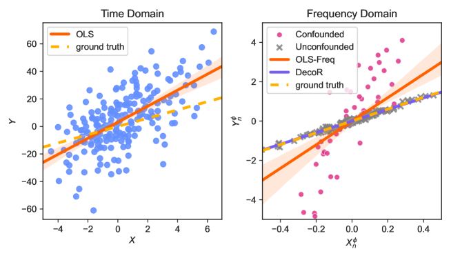
Figure 1: Due to the hidden confounder, regressing $Y$ on $X$ in the time-domain (left) does not yield a consistent estimator of the true causal effect (dashed, yellow). The idea of DecoR (green, see Section 2.1) is to consider the data in the frequency domain. Even though it is unknown, which of the data points correspond to confounded (orange) and unconfounded (gray) frequencies, robust regression techniques can be used to estimate the causal effect. We prove that DecoR is consistent under weak assumptions if the confounding is sparse, see Section 3.

2 Sparse Representation for Deconfounding

We now formalize the underlying model assumptions and the methodological procedure.

Setting 1.

Let $d\in\mathbb{N}$ and let $T\in\mathbb{R}_{>0}$ denote a fixed time horizon. Let $X=(X_{t})_{t\in[0,T]}$ be a stochastic process in $\mathbb{R}^{d}$ and $U=(U_{t})_{t\in[0,T]}$ a stochastic process in $\mathbb{R}$. Let $\eta=(\eta_{t})_{t\in[0,T]}$ be a process of i.i.d. centered Gaussian random variables independent of $X$ and with constant variance $\sigma^{2}_{\eta}\geq 0$. Let $\beta\in\mathbb{R}^{d}$ and let $Y=(Y_{t})_{t\in[0,T]}$ be a stochastic process that satisfies

$$Y_{t}=X_{t}^{\top}\beta+U_{t}+\eta_{t}.$$

Fix $n\in\mathbb{N}$. We assume that we observe $X^{n}\coloneqq(X_{T/n},X_{2T/{n}},\dots,X_{T})$ and $Y^{n}:=(Y_{T/n},Y_{2T/{n}},\dots,Y_{T})$.

We assume Setting 1 for the remainder of this section and consider the goal of estimating $\beta$ from $X^{n}$ and $Y^{n}$. Setting 1 does not require any underlying causal model and $\beta$ is an interesting target of inference from a regression point of view. However, the set-up is particularly relevant if $\beta\in\mathbb{R}$ is the total causal effect of $X_{t}$ on $Y_{t}$, that is, $\beta=\frac{\partial}{\partial x}\mathbb{E}[Y_{t}\ |\ \mathrm{do}(X_{t}=x)]$ for all $t\in[0,T]$ (Pearl, 2009). In the most basic scenario, $U$ acts as a confounder, effecting $Y$ through a linear relationship while its effect on $X$ can be non-linear. We illustrate this scenario in Figure 2.

However, Setting 1 is more general than the additive structure may initially suggest. In particular, we show that it suffices to assume that $Y_{t}=X_{t}^{\top}\beta+\epsilon_{t}$ for some (not necessarily uncorrelated) stochastic processes $X$ and $\epsilon$; for details, see Appendix B.

Consider a (known) orthonormal basis $\phi=\{\phi_{k}\}_{k\in\mathbb{N}}$ of $L^{2}([0,T])$. We typically choose the cosine basis (see Definition C.1) as $\phi$ in our applications. The main assumption of this paper is that the confounder is sparse in this basis.

Definition 2.1 ($(\phi,G)$-sparse process ).

Let $G\subseteq\mathbb{N}$ and let $U=(U_{t})_{t\in[0,T]}$ be a stochastic process in $\mathbb{R}$ satisfying $\mathbb{E}[\int_{0}^{T}U_{t}^{2}dt]<\infty$. If for all $k\notin G$ almost surely

$$\langle U,\phi_{k}\rangle_{L^{2}}=0,$$

we call $U$ a $(\phi,G)$-sparse process.

Assumption 1 (Sparse confounding assumption).

The set $G\subseteq\mathbb{N}$ is such that $U$ is a $(\phi,G)$-sparse process.

The theoretical results presented in the remainder of this paper explicitly assume Assumption 1 to hold for a $G$ with suitable properties (informally speaking, for ‘small’ $G$).

Figure 2: Directed acyclic graph covered by Setting 1. The dashed arrow from $U_{t}$ to $Y_{t}$ indicates that we assume $U_{t}$ to be sparse and the effect on $Y_{t}$ to be additive,

To see how this sparsity can exploited, let $\mathcal{S}$ be the set of $\mathbb{R}^{d}$-valued stochastic processes on $[0,T]$ and $\mathcal{C}$ the set of random variables on $\mathbb{R}^{d}$. Define, for all $k\leq n$, the function $T_{k}^{\phi,n}:\mathcal{S}\to\mathcal{C}$ by

$$T_{k}^{\phi,n}(V)\coloneqq\begin{bmatrix}\frac{1}{n}\sum_{l=1}^{n}(V_{Tl/n})_{1}\phi_{k}(Tl/n)\\ \vdots\\ \frac{1}{n}\sum_{l=1}^{n}(V_{Tl/n})_{d}\phi_{k}(Tl/n)\end{bmatrix}.$$ (1)

For the cosine basis, Equation (1) corresponds to taking the discrete cosine transform (applied to $V_{T/n},\ldots,V_{T}$). Using the linearity of $T_{k}^{\phi,n}$, it holds for all $k\leq n$

$$\begin{split}T_{k}^{\phi,n}(Y)&=T_{k}^{\phi,n}(X)^{\top}\beta+T_{k}^{\phi,n}(U)+T_{k}^{\phi,n}(\eta)\\ &\overset{\text{a.s.}}{=}\begin{cases}T_{k}^{\phi,n}(X)^{\top}\beta+T_{k}^{\phi,n}(U)+T_{k}^{\phi,n}(\eta)&\text{if }k\in G,\\ T_{k}^{\phi,n}(X)^{\top}\beta+T_{k}^{\phi,n}(\eta)&\text{if }k\notin G.\end{cases}\end{split}$$ (2)

Equation (2) makes use of a technical condition on the transformation; see Assumption 2(i) and its discussion in Section 4.

The core idea is to consider the pairs $\{(T_{k}^{\phi,n}(X),T_{k}^{\phi,n}(Y))\}_{k\leq n}$ as a new data set and to observe that by Assumption 1 only the data points with an index $k\in G$ are confounded. If $G$ is known or if there exists a known subset $S\subseteq\mathbb{N}$ with $G\subseteq S$, the unconfounded dataset $\{(T_{k}^{\phi,n}(X),T_{k}^{\phi,n}(Y))\}_{k\notin S}$ can be analyzed using standard linear inference methods to, for example, consistently estimate $\beta$. However, in many cases, $G$ (or $S$) might be unknown. In the next section, we introduce DecoR, an algorithm for estimating $\beta$ without assuming knowledge of $G$ but assuming sparsity instead.

2.1 DecoR: Deconfounding by Robust Regression

The key insight exploited in this section is the identification of (2) as an adversarial outlier problem. We define $X^{n}_{\phi}\coloneqq(T_{1}^{\phi,n}(X),\dots,T_{n}^{\phi,n}(X))^{\top}$ and similarly for $Y^{n}_{\phi}$ and $\eta^{n}_{\phi}$, and $o^{n}_{\phi}$ as $o^{n}_{\phi}\coloneqq(T_{1}^{\phi,n}(U),\dots,T_{n}^{\phi,n}(U))^{\top}$. This reformulation allows us to express the relationship (2) as:

$$Y^{n}_{\phi}=X^{n}_{\phi}\beta+\eta^{n}_{\phi}+o^{n}_{\phi}.$$ (3)

The outlier vector $o^{n}_{\phi}$ may exhibit dependence on $X$. However, because of Assumption 1 we know that for all indices $k$ not in $G$, the component $(o^{n}_{\phi})_{k}$ equals $0$. This scenario mirrors a linear regression model with adversarial outliers, a challenge well-studied in robust statistics literature (see, e.g., Bhatia et al., 2015). To estimate $\beta$ we can thus apply robust linear regression to (3). We call this methodology DecoR and outline the full procedure in Algorithm 1. While it can be paired with any adversarial robust linear regression algorithm, in our experiments, we have used Torrent (Bhatia et al., 2015). Figure 4 in Appendix A offers a graphical illustration of the method, emphasizing the transition from time-domain data to frequency-domain analysis and the subsequent application of a robust regression algorithm.

Algorithm 1 DecoR

$X^{n}\in\mathbb{R}^{n\times d}$, $Y^{n}\in\mathbb{R}^{n}$, orthonormal basis $\phi$, robust linear regression algorithm $\mathcal{A}$

$X^{n}_{\phi}\leftarrow(T_{1}^{\phi,n}(X),\dots,T_{n}^{\phi,n}(X))^{\top}$ $\triangleright$ See (1)

$Y^{n}_{\phi}\leftarrow(T_{1}^{\phi,n}(Y),\dots,T_{n}^{\phi,n}(Y))^{\top}$

$\hat{\beta}^{\phi,n}_{\texttt{DecoR}}\leftarrow\mathcal{A}(X^{n}_{\phi},Y^{n}_{\phi})$

return $\hat{\beta}^{\phi,n}_{\texttt{DecoR}}$

In Section 3 we introduce the robust linear regression with adversarial outliers problem, discuss the robust algorithms BFS and Torrent and provide novel theoretical guarantees for their estimation errors. In Section 4 we use these results to provide conditions under which the estimator returned by DecoR is consistent.

3 Theoretical Guarantees for Robust Regression

We first introduce the setting of a linear model with adversarial outliers, which we assume for the remainder of Section 3.

Setting 2.

Let $d\in\mathbb{N}$ and $\beta\in\mathbb{R}^{d}$. For all $n\geq d$, let $\epsilon\in\mathbb{R}^{n}$, $X\in\mathbb{R}^{n\times d}$ and $G_{n}\subseteq\{1,\ldots,n\}$ and let $o\in\mathbb{R}^{n}$ be such that $\forall i\notin G_{n}:o_{i}=0$. Define $Y\in\mathbb{R}^{n}$ by

$$Y\coloneqq X\beta+\epsilon+o.$$ (4)

We call $G_{n}$ the (potential) outliers and $G_{n}^{\mathsf{c}}$ the inliers. We observe $X$ and $Y$. The goal is to estimate $\beta$.

Setting 2 describes the adversarial outlier setting. In particular, $o$ can depend on $X$. For any $S\subseteq\{1,\ldots,n\}$, we denote by $X_{S}\in\mathbb{R}^{|S|\times d}$ the submatrix of $X$ that only includes rows with indices in $S$ (for $S=\emptyset$, this is the empty matrix, whose rank equals zero). We similarly denote the subvectors of $Y,\epsilon$ and $o$ that only includes rows with indices in $S$ by $Y_{S},\epsilon_{S}$ and $o_{S}$. If $\operatorname{rank}(X_{S})\geq d$, we denote by

$$\hat{\beta}^{S}_{\texttt{OLS}}(X,Y)\coloneqq(X_{S}^{\top}X_{S})^{-1}X_{S}^{\top}Y_{S}$$ (5)

the ordinary-least-squares estimator. We often write $\hat{\beta}^{S}_{\texttt{OLS}}$ instead of $\hat{\beta}^{S}_{\texttt{OLS}}(X,Y)$ when $X,Y$ is apparent from the context. We also write $\hat{\beta}_{\texttt{OLS}}(X,Y)\coloneqq\hat{\beta}^{\{1,\dots,n\}}_{\texttt{OLS}}(X,Y)$.

This work discusses two algorithms for estimating $\beta$ in (4), both of these methods include some form of linear regression. Algorithm 2 takes as input a collection $\mathcal{U}_{n}$ of candidate sets for the inliers $G_{n}^{\mathsf{c}}$. For example, we might have knowledge of an upper bound $a$ for the number of outliers. We can then define $\mathcal{U}_{n}=\{S\subseteq\{1,\dots,n\}\ |\ |S|\geq n-a\}$. We can then search over all elements in $\mathcal{U}_{n}$, compute the OLS estimate on the corresponding data and choose the estimate with the smallest prediction error. We call this method Brute Force Search (BFS) and detail it in Algorithm 2. We will see in Section 3.1 that if, indeed, $G_{n}^{\mathsf{c}}\in\mathcal{U}_{n}$, the procedure is consistent under suitable assumptions.

Algorithm 2 BFS

$X\in\mathbb{R}^{n}$, $Y\in\mathbb{R}^{n},\mathcal{U}_{n}$

$\hat{\beta}^{n}_{\texttt{BFS}}(\mathcal{U}_{n})\leftarrow 0$, $\mathrm{err}_{0}\leftarrow\infty$

for $S\in\mathcal{U}_{n}$ do

     $\mathrm{err}_{1}\leftarrow\frac{1}{|S|}\left\lVert Y_{S}-X_{S}\hat{\beta}^{S}_{\texttt{OLS}}(X,Y)\right\rVert^{2}_{2}$ $\triangleright$ see (5)

     if $\mathrm{err}_{1}<\mathrm{err}_{0}$ then

         $\hat{\beta}^{n}_{\texttt{BFS}}(\mathcal{U}_{n})\leftarrow\hat{\beta}_{S}$

         $\mathrm{err}_{0}\leftarrow\mathrm{err}_{1}$

     end if

end for

return $\hat{\beta}^{n}_{\texttt{BFS}}(\mathcal{U}_{n})$

Algorithm 2 is computationally expensive unless $\mathcal{U}_{n}$ contains only few sets. In practice, Torrent (Bhatia et al., 2015) is an often computationally more efficient method for estimating $\beta$. For all $v\in\mathbb{R}^{n}$ let $s_{1},\dots,s_{n}$ be the unique permutation of $\{1,\dots,n\}$ such that $v_{s_{1}}\leq v_{s_{2}}\leq\dots\leq v_{s_{n}}$, where ties are broken with a fixed deterministic rule. Further, define for $a\in\{1,\dots,n\}$ the set

$$\mathrm{HT}(v,a)\coloneqq\{s_{1},\dots,s_{a}\}$$ (6)

containing the indices corresponding to the $a$ smallest entries of $v$ (‘HT’ stands for ‘hard-threshold’). With this notation Torrent is defined as in Algorithm 3.

Algorithm 3 Torrent (Bhatia et al., 2015)

$X\in\mathbb{R}^{n\times d}$, $Y\in\mathbb{R}^{n}$, $a\in\{1,\dots,n\}$

$S_{0}\leftarrow\{1,\dots,n\}$, $e\leftarrow Y$, $\mathrm{err}\leftarrow\infty$, $t\leftarrow 0$

while $\left\lVert e\right\rVert_{2}<\mathrm{err}$ do

     $t\leftarrow t+1$

     $\mathrm{err}\leftarrow\left\lVert e\right\rVert_{2}$

     $\hat{\beta}^{t}_{\texttt{Tor}}\leftarrow\hat{\beta}^{S_{t-1}}_{\texttt{OLS}}(X,Y)$ $\triangleright$ see (5)

     $e\leftarrow|Y-X\hat{\beta}^{t}_{\texttt{Tor}}|$

     $S_{t}\leftarrow\mathrm{HT}(e,a)$ $\triangleright$ see (6)

end while

return $\hat{\beta}^{n,a}_{\texttt{Tor}}:=\hat{\beta}^{t}_{\texttt{Tor}}$

3.1 Guarantees for BFS

Let $\mathcal{U}_{n}\subseteq\mathcal{P}(\{1,\dots,n\})$, $\emptyset\notin\mathcal{U}_{n}$, be the collection of candidate sets for the inliers $\mathcal{U}_{n}$ that we use as an input for Algorithm 2 and let us denote the algorithm’s output by $\hat{\beta}^{n}_{\texttt{BFS}}(\mathcal{U}_{n})$. Furthermore, we define

$$\mathrm{Inl}(\mathcal{U}_{n})\coloneqq\{S\in\mathcal{U}_{n}\ |\ S\cap G_{n}=\emptyset\},$$

denoting the collection of sets in $\mathcal{U}_{n}$ that do not contain any outliers. We can now prove the following result about BFS.

Theorem 3.1.

Assume Setting 2 with $d=1$ and that $\mathrm{Inl}(\mathcal{U}_{n})\neq\emptyset$. Assume that $\epsilon_{1},\ldots,\epsilon_{n}$ are i.i.d. zero-mean Gaussians with variance $\sigma^{2}\geq 0$. Define for all $S\in\mathcal{U}_{n}$, and $U_{n}\in\mathrm{Inl}(\mathcal{U}_{n})$,

$$\alpha_{1}(S,U_{n},\delta)\coloneqq\frac{|S|}{{|U_{n}|}}\left(\sigma\sqrt{|U_{n}|}+\sigma\sqrt{K\log(2|\mathcal{U}_{n}|/\delta)}\right)^{2}-\left(\sigma\sqrt{|S|}-\sigma\sqrt{K\log(2|\mathcal{U}_{n}|/\delta)}\right)^{2},$$

where $K>0$ is the constant from Lemma D.1, and define

$$\alpha(S,U_{n},\delta) \coloneqq\frac{4\sigma\left\lVert X_{{S}}\right\rVert_{2}\sqrt{2\log(2|\mathcal{U}_{n}|/\delta)}}{\left\lVert X_{{S}\setminus G_{n}}\right\rVert_{2}^{2}}+\frac{\sqrt{\alpha_{1}(S,U_{n},\delta)}}{\left\lVert X_{{S}\setminus G_{n}}\right\rVert_{2}}+\frac{\sigma\sqrt{2\log(2|\mathcal{U}_{n}|/\delta)}}{\left\lVert X_{{S}\setminus G_{n}}\right\rVert_{2}}.$$

Let $\delta>0$. Then, with probability at least $1-\delta$ it holds that

$$\left|\hat{\beta}^{n}_{\texttt{BFS}}(\mathcal{U}_{n})-\beta\right|\leq\max_{S\in\mathcal{U}_{n}}\min_{U_{n}\in\mathrm{Inl}(\mathcal{U}_{n})}\left\{\alpha(S,U_{n},\delta)+\frac{\sigma\sqrt{2\log(6|\mathcal{U}_{n}|/\delta)}}{\left\lVert X_{S}\right\rVert_{2}}\right\}.$$

The proof can be found in Appendix D.2. Theorem 3.1 implies that BFS is consistent if the noise variance $\sigma^{2}$ is equal to $0$ and $\min_{S\in\mathcal{U}_{n}}||X_{S\setminus G_{n}}||_{2}\neq 0$, implying that $\mathcal{U}_{n}$ does not contain any subsets of $G_{n}$. Furthermore, it shows that if the fraction of outliers is vanishing with increasing $n$, BFS is consistent under mild assumptions on the collection $\mathcal{U}_{n}$ of candidate sets; it suffices, for example, if the distribution of $X$ is such that, with high probability,

$$\min_{S\in\mathcal{U}_{n}}||X_{S\setminus G_{n}}||_{2}\in\Omega(\sqrt{n}),\qquad\max_{S\in\mathcal{U}_{n}}||X_{S}||_{2}\in\mathcal{O}(\sqrt{n})$$ (7)

and if $\mathcal{U}_{n}$ is chosen such that

$$\max_{S\in\mathcal{U}_{n}}\min_{U_{n}\in\mathrm{Inl}(\mathcal{U}_{n})}\sqrt{|S|\log(|\mathcal{U}_{n}|)/\sqrt{|U_{n}|}}\in o(\sqrt{n}).$$ (8)

For details, see Appendix E.2. Conditions (8) and (7) hold, for example, when we have a known sequence $\{c_{n}\}_{n\in\mathbb{N}}$ such that, for all $n$, $|G_{n}|\leq c_{n}$ and $c_{n}$ $\in o(\sqrt{n}/\log(n))$, we define the collection of candidate sets as $\mathcal{U}_{n}\coloneqq\{S\in\mathcal{P}(\{1,\dots,n\})\mid|S|=n-c_{n}\}$ and the rows of $X$ are i.i.d. Gaussian, see Bhatia et al. (2015, Theorem 15). If the fraction of outliers is non-vanishing (and $c_{n}<n/2$), Theorem 3.1 implies that for a distribution of $X$ satisfying (7) and the same choice of candidate sets defined by $\mathcal{U}_{n}\coloneqq\{S\in\mathcal{P}(\{1,\dots,n\})\mid|S|=n-c_{n}\}$, that $|\hat{\beta}^{n}_{\texttt{BFS}}(\mathcal{U}_{n})-\beta|\in\mathcal{O}(\sigma)$. Theorem 3.1 implies uniform consistency results, too. For example, in the case of $\sigma=0$, we obtain uniform consistency even over classes of distributions with outliers that shift the original data points by an arbitrary amount. On the contrary, regression that is based on a robust loss function, such as the Huber loss (Huber, 1964), does not come with similar guarantees, not even with respect to pointwise consistency or in the case $\sigma=0$.

3.2 Guarantees for Torrent

In this section we strengthen existing bounds for the estimation error of Torrent by improving the result of Bhatia et al. (2015, Theorem 10).

Lemma 3.2.

For all $n\in\mathbb{N}$ there is a constant $N\in\mathbb{N}$ such that Algorithm 3 converges in less than $N$ steps.

In practice, we observe that Torrent requires only very few interrations until it convergences (cf. Table 8). We can use Lemma 3.2 to obtain an improved guarantee for Algorithm 3.

Theorem 3.3.

Assume Setting 2. Assume that there exists a known $c_{n}\in\mathbb{N}$ such that $|G_{n}|\leq c_{n}$. Let $S_{t}$ be the estimated subset in the final iteration of Algorithm 3 executed on the data $X$, $Y$ using threshold parameter $a_{n}\coloneqq n-c_{n}$. Define for $S\subseteq\{1,\dots,n\}$

$$V(S)\coloneqq(S\cup G_{n}^{\mathsf{c}})\setminus(G_{n}^{\mathsf{c}}\cap S),$$

the symmetric difference between $S$ and $G_{n}^{\mathsf{c}}$. Furthermore, assume that

$$\eta\coloneqq\max_{S\subseteq\{1,\dots,n\}\text{ s.t. }|S|=a_{n}}\frac{\left\lVert X_{V(S)}\right\rVert_{2}}{\sqrt{\lambda_{\mathrm{min}}\left(X_{S}^{T}X_{S}\right)}}<\frac{1}{\sqrt{2}}.$$

Then

$$\left\lVert\hat{\beta}^{n,a_{n}}_{\texttt{Tor}}-\beta\right\rVert_{2}\leq\left\lVert\left(X_{S_{t}}^{\top}X_{S_{t}}\right)^{-1}X_{S_{t}}^{\top}\epsilon_{S_{t}}\right\rVert_{2}+\frac{2\left\lVert X_{V(S_{t})}\right\rVert_{2}\left\lVert\left(X_{S_{t}}^{\top}X_{S_{t}}\right)^{-1}X_{S_{t}}^{\top}\epsilon_{S_{t}}\right\rVert_{2}+\sqrt{2}\|\epsilon_{V(S_{t})}\|_{2}}{\sqrt{\lambda_{\mathrm{min}}\left(X_{S_{t}}^{T}X_{S_{t}}\right)}\left(1-\sqrt{2}\eta\right)}.$$

The proof can be found in Appendix D.4. Defining

$$\lambda_{a_{n}}(X)\coloneqq\min_{S\subseteq\{1,\dots,n\}\text{ s.t. }|S|=a_{n}}\sqrt{\lambda_{\mathrm{min}}\left(X_{S}^{T}X_{S}\right)}$$

we can use this result to derive an upper bound for the estimation error in the sub-Gaussian noise setting.

Corollary 3.4 (sub-Gaussian noise).

Assume the setting of Theorem 3.3 with i.i.d. zero-mean sub-Gaussian noise $\epsilon$ with variance proxy $\sigma^{2}$ and assume $c_{n}<n/2$. Then, there exists a constant $K>0$ such that for all $\delta>0$ with probability at least $1-\delta$

$$\left\lVert\hat{\beta}^{n,a_{n}}_{\texttt{Tor}}-\beta\right\rVert_{2} \leq\frac{\sigma}{\lambda_{a_{n}}(X)}\left(1+\frac{\sqrt{2}}{1-\sqrt{2}\eta}\right)\left(\sqrt{d}+\sqrt{2c_{n}K\log(2en/c_{n}\delta)}\right)+\frac{2\sigma\sqrt{c_{n}}\left(1+\sqrt{K\log(2en/c_{n}\delta)}\right)}{\lambda_{a_{n}}(X)(1-\sqrt{2}\eta)}.$$

In particular, if the rows of $X$ are i.i.d. standard Gaussian random vectors and $c_{n}\in o(n/\log(n))$, then $\hat{\beta}^{n,a_{n}}_{\texttt{Tor}}$ is consistent.

While Corollary 3.4 states consistency under appropriate conditions and vanishing fractions of outliers, the results in Bhatia et al. (2015) are not sufficiently strong to imply consistency in this setting. Furthermore, even for non-vanishing fraction of outliers our bounds are in general tighter since the maximum over $S$ in the definition of $\eta$ is taken jointly over the denominator and numerator, not separately as in Bhatia et al. (2015).

4 Guarantees for DecoR

We can now prove bounds for the estimation error of DecoR. Let $(\Omega,\mathcal{F},\mathbb{P})$ be a probability space and let $T\in\mathbb{R}_{>0}$ denote a fixed time horizon. Denote by $\mathcal{M}^{2}_{[0,T]}$ the set of measurable, real valued, square integrable stochastic processes, that is, all Lebesgue-measurable, real-valued stochastic processes $(V_{t})_{t\in[0,T]}$ that satisfy $\mathbb{E}[\int_{0}^{T}V_{t}^{2}dt]<\infty$. For all $\phi=\{\phi_{k}\}_{k\in\mathbb{N}}$ orthonormal bases of $L^{2}([0,T])$ and all $V=(V_{t})_{t\in[0,T]}\in\mathcal{M}^{2}_{[0,T]}$, we have $\int_{0}^{T}V_{t}^{2}dt<\infty$ almost surely and, therefore, $\langle V,\phi_{k}\rangle_{L_{2}}$ exists almost surely.

For the remainder of this section we assume Setting 1 and that Assumption 1 is satisfied for $G$ and $\phi$. More precisely, let $G\subseteq\mathbb{N}$, let $\phi=\{\phi_{k}\}_{k\in\mathbb{N}}$ be an orthonormal basis of $L^{2}([0,T])$, let $U=(U_{t})_{t\in[0,T]}\in\mathcal{M}^{2}_{[0,T]}$ be a $(\phi,G)$-sparse process and let $X=(X_{t})_{t\in[0,T]}$ be a stochastic process in $\mathbb{R}^{d}$. Let $\eta=(\eta_{j})_{j\in[0,T]}$ be a stochastic process of i.i.d. centered Gaussian random variables with variance $\sigma_{\eta}^{2}\geq 0$ and let $Y_{t}$ be a stochastic process, such that, for all $t\in[0,T]$,

$$Y_{t}\coloneqq X_{t}^{\top}\beta+U_{t}+\eta_{t}.$$

We also assume some regularity conditions on $\phi$ and $U$. Specifically, we assume that for all $k\in\mathbb{N}$ it holds that $\phi_{k}$ is right-continuous (or left-continuous) and that the trajectories of $U$ satisfy the same condition almost surely. This implies that, almost surely, for all $t\in[0,T]$

$$U_{t}=\sum_{k\in G}\langle\phi_{k},U\rangle_{L^{2}}\phi_{k}(t).$$ (9)

As described in Setting 1,we assume that, for $n\in\mathbb{N}$, we observe $X^{n}\coloneqq(X_{T/n},X_{2T/{n}},\dots,X_{T})$ and $Y^{n}:=(Y_{T/n},Y_{2T/{n}},\dots,Y_{T})$. We consider the transformation $T_{k}^{\phi,n}$, see (1), and write $X^{n}_{\phi}\coloneqq(T_{1}^{\phi,n}(X),\dots,T_{n}^{\phi,n}(X))^{\top}$ (see also Algorithm 1) and $G_{n}\coloneqq G\cap\{1,\dots,n\}$.

The theoretical results presented in this section are based on two types of assumptions. One assumption ensures that $G_{n}$ does not grow too quickly with $n$ (clearly, if $|G_{n}|\geq n/2$, for example, there is no consistent estimator for $\beta$). Another set of assumptions contains technical conditions on the transformation $T^{\phi,n}$, see (1) and (2).

Assumption 2.

1. For all $n\in\mathbb{N}$ and $l,k\leq n$ it holds that $\frac{1}{n}\sum_{j=1}^{n}\phi_{l}(Tj/n)\phi_{k}(Tj/n)=\mathbbm{1}{\{l=k\}}$.

2. For every $\delta>0$ there exists $c^{\prime}>0$ and $\bar{n}\in\mathbb{N}$ such that for all $n\geq\bar{n}$ there exists $S^{\prime}_{n}\subseteq\{1,\dots,n\}$ with $|S^{\prime}_{n}|=2c_{n}+d$ such that for all $S^{\prime\prime}\subset S^{\prime}_{n}$ with $|S^{\prime\prime}|=d$ it holds that with probability at least $1-\delta$

   $$\lambda_{\mathrm{min}}\left((X^{n}_{\phi})_{S^{\prime\prime}}^{\top}(X^{n}_{\phi})_{S^{\prime\prime}}\right)\geq c^{\prime}.$$

Assumption 2 (i) states that the chosen orthonormal basis maintains its orthogonality and normalization properties when applied to discretized observations; this is satisfied, for example, by the cosine basis or the Haar basis (Haar, 1909), see Appendix C. Together with (9), this implies (2). Assumption 2 (ii) requires that $X$ is non-sparse in the $\phi$-domain. This condition intuitively says that there is more information in $X$ than is lost by confounding. This condition is relatively mild and accommodates a wide array of commonly used stochastic processes, including Ornstein-Uhlenbeck processes, Brownian motions, and band-limited processes. We are now able to state the main theoretical results, the convergence properties of DecoR-BFS (DecoR with BFS as robust regression algorithm) and DecoR-Tor (DecoR with Tor as robust regression algorithm).

Theorem 4.1 (Convergence properties of DecoR-BFS).

Let $c_{n}$ be a known sequence of natural numbers such that $|G_{n}|\leq c_{n}$ and let Assumption 2 be satisfied. Assume that $d=1$, that $U$ is independent of $\epsilon$, that $\sup_{t\in[0,T]}\mathbb{E}[X_{t}^{2}]<\infty$ and that for all $n\in\mathbb{N}$ and $j,i\leq T$ it holds that $\frac{1}{n}\sum_{l=1}^{n}\phi_{l}(Tj/n)\phi_{l}(Ti/n)=\mathbbm{1}{\{i=j\}}$. Define a sequence of candidate sets by $\mathcal{U}_{n}:=\{S\subseteq\{1,\dots,n\}\ |\ |S|=n-c_{n}\}$. If DecoR is executed with BFS and the sequence of sample sets $\mathcal{U}_{n}$, then there exists $\bar{n}\in\mathbb{N}$ such that for all $n\geq\bar{n}$ with high probability

$$\left|\hat{\beta}^{\phi,n}_{\texttt{DecoR}}-\beta\right|\in\mathcal{O}\left(\sigma_{\eta}\left(\frac{c_{n}\log(n/c_{n})}{n}\right)^{1/4}\right).$$

Many commonly used bases, such as the cosine basis and the Haar basis, satisfy the conditions of Theorem 4.1.

Theorem 4.2 (Convergence properties of DecoR-Tor).

Let $c_{n}$ be a known sequence of natural numbers such that $|G_{n}|\leq c_{n}$ and let Assumption 2 be satisfied. Assume that for all $\delta>0$ there exists $\bar{n}\in\mathbb{N}$ such that for all $n\geq\bar{n}$ it holds that

$$\mathbb{P}\left[\max_{S\subseteq\{1,\dots,n\}\text{ s.t. }|S|=n-c_{n}}\frac{\left\lVert(X^{n}_{\phi})_{V(S)}\right\rVert_{2}}{\sqrt{\lambda_{\mathrm{min}}\left((X^{n}_{\phi})_{S}^{T}(X^{n}_{\phi})_{S}\right)}}<\frac{1}{\sqrt{2}}\right]\geq 1-\delta.$$ (10)

If DecoR is executed with Torrent and the sequence of threshold parameters $a_{n}=n-c_{n}$, then there exists $\bar{n}\in\mathbb{N}$ such that for all $n\geq\bar{n}$ with high probability

$$\left\lVert\hat{\beta}^{\phi,n}_{\texttt{DecoR}}-\beta\right\rVert_{2} \in\mathcal{O}\left(\sigma_{\eta}\sqrt{\frac{c_{n}\log(n/c_{n})}{n}}\right).$$

If the assumptions of Theorem 4.1 or Theorem 4.2 are satisfied and either there is no noise, that is, $\sigma_{\eta}=0$, or the number of confounded components $c_{n}$ grows more slowly than the sample size $n$, that is, $c_{n}\in o(n)$, then DecoR produces a consistent estimator for $\beta$. Conversely, if there is non-zero noise and the number of confounded components $c_{n}$ is asymptotically proportional to $n$, that is, $c_{n}\sim n$, the estimation error of DecoR is asymptotically bounded by the noise variance $\sigma_{\eta}$, up to constant factors. While DecoR-Tor has polynomial-time complexity and in our experiments converges very fast (cf. Table 8), the theoretical result (Theorem 4.2) contains stronger theoretical assumptions than the one based on BFS (Theorem 4.1) , specifically it requires (10) to hold. In contrast, DecoR-BFS does not require (10), but its computational complexity is exponential in $n$ when $c_{n}$ is not bounded by a constant.

In the next section, we show that when $X$ and $U$ are band-limited processes, DecoR can be consistent, even for a constant fraction of outliers.

4.1 Example: Band-Limited Processes

Let $\{\phi_{k}\}_{k\in\mathbb{N}}$ be a basis of $L^{2}([0,T])$ and let $S\subset\mathbb{N}$ be a bounded set. We call a real-valued stochastic process $V$ an $(S,\phi)$ band-limited process if there exists a set of random variables $\{a^{V}_{k}\}_{k\in S}$ with finite second moments such that, almost surely,

$$V=\sum_{k\in S}a^{V}_{k}\phi_{k}.$$

Let $S_{X},S_{U}\subset\mathbb{N}$ be bounded sets and assume that $X$ is a $(S_{X},\phi)$ band-limited process and that $U$ is a $(S_{U},\phi)$ band-limited process. Assume $\phi$ satisfies Assumption 2 (i). Then, for all $k,n\in\mathbb{N}$, we have almost surely that

$$(X^{\phi}_{n})_{k}=\begin{cases}a^{X}_{k}&\text{if $k\in S_{X}$}\\ 0&\text{if $k\notin S_{X}$}\end{cases}$$

and analogously for $U$. Let $c\coloneqq|S_{X}\cap S_{U}|$ and assume that $|S_{X}|\geq 2c+1$. Assume further that, there exists $r>0$ such that for all $k\in S_{X}$ it holds that almost surely $|a_{k}^{U}|\geq r$. This implies Assumption 2 (ii) and therefore, by Theorem 4.1, DecoR-BFS is consistent. If, additionally, condition (10) is satisfied – this is the case with high probability, for example, if $\{a_{k}^{X}\}_{k\in S_{X}}$ are i.i.d. Gaussian and $|S_{X}|$ is large – then, by Theorem 4.2, DecoR-Tor is also consistent. Moreover, OLS can be inconsistent in this setting, as shown in the following proposition.

Proposition 4.3.

Assume Setting 1 and assume Assumption 2 holds. Then, $\hat{\beta}^{\phi,n}_{\texttt{OLS}}$ is not necessarily a consistent estimator for $\beta$. Even if $X$ is a band-limited process, OLS may be inconsistent.

We regard these results surprising in that they describe a setting, in which the number of outliers increases linearly in $n$ and there is a constant noise variance, and still robust regression yields a consistent estimator (and OLS does not). As discussed in Appendix E.3 such an estimator does not exist for i.i.d. data.

5 Empirical Evaluation

We validate our theoretical findings through experiments on synthetic data. In the experiments, we generate data according to the model described in Setting 1 and set $X\coloneqq U+\epsilon_{X}$. We sample $\epsilon_{X}$ and $U$ from either two independent Ornstein-Uhlenbeck processes or two independent band-limited processes. For the orthogonal basis $\phi$, we consider both the cosine basis (see Definition C.1) and the Haar basis (see Definition C.2). The noise in $Y$ is set to have variance $\sigma_{\eta}^{2}\in\{0,1,4\}$. To assess the accuracy of the different approaches, we calculate the mean absolute prediction error: $\mathrm{MAE}\coloneqq\sum_{i=1}^{n}|\beta_{i}-\hat{\beta}^{n}_{i}|/n$. For the remainder of this section, if not specified otherwise, we assume independent band-limited processes, the cosine basis, noise variance of $\sigma^{2}_{\eta}=1$, fraction of outliers of $25\%$ and $a=0.7$. Detailed information on the experimental setup is available in Appendix F.2 and code has been made available at https://github.com/fschur/robust_deconfounding.

$n$	$\sigma_{\eta}^{2}$	OLS	DecoR-Tor	DecoR-BFS
8	0	1.69 (0.05)	0.32 (0.04)	0.00 (0.00)
12	0	1.70 (0.05)	0.13 (0.02)	0.00 (0.00)
16	0	1.66 (0.04)	0.06 (0.02)	0.00 (0.00)
8	1	1.70 (0.05)	0.55 (0.03)	0.24 (0.01)
12	1	1.71 (0.05)	0.33 (0.02)	0.17 (0.01)
16	1	1.67 (0.04)	0.21 (0.01)	0.14 (0.00)

Table 1: Comparison of the mean absolute estimation error (with standard deviation of the mean in parenthesis) between OLS, DecoR-BFS and DecoR-Tor. For more than $16$ data points BFS becomes computationally infeasible.

We first compare the average estimation error of OLS, DecoR-Tor and DecoR-BFS. As discussed in Section 3, the computation time of DecoR-BFS scales exponentially with the sample size $n$, so we only consider sample sizes up to $n=16$. Table 1 shows the results. In the absence of noise, that is, if $\sigma^{2}_{\eta}=0$, DecoR-BFS correctly point-identifies the true parameter $\beta$ for all samples sizes – this is in agreement with Theorem 4.1. Although the average estimation error of DecoR-Tor decreases as the sample size increases, it does not reach zero, unlike the estimation error of DecoR-BFS. This discrepancy arises because condition (10) is often not satisfied in smaller sample sizes (not shown). The discrepancy also suggests a trade-off between computational costs and average estimation error. Since DecoR is modular in that it can be applied with any robust regression technique, it directly benefits from any methodological advancement in the field of robust regression. As expected, the estimation error for OLS remains constant regardless of sample size and is significantly larger than that of both DecoR-Tor and DecoR-BFS.

In Section 4.1 we have shown that under suitable conditions DecoR is consistent when $U$ and $X$ are band-limited processes. Figure 3 (left) shows that the mean absolute estimation error for processes from this class vanishes with growing sample size, supporting considers Ornstein-Uhlenbeck processes and suggests that DecoR might also be consistent for this class of processes. We show, however, in Appendix E.3 that there are settings with Ornstein-Uhlenbeck processes where no consistent estimator exists; it therefore seems that many of the cases in Figure 3 (right) contain confounding that is not worst-case, so DecoR is still consistent. In both cases (Figure 3 (left) and Figure 3 (right)) the error of OLS does not seem to vanish with growing sample size.

We present additional experimental results in Appendix F.2. Figure 5 and Figure 7 suggest that DecoR-Tor is consistent in the setting where the Haar basis is used in place of the cosine basis, and in the setting where $X$ is two-dimensional. Furthermore, Figure 6 investigates consistency of DecoR-Tor under model misspecification; more specifically, we consider a growing fraction of confounded components and a model introducing Gaussian noise to $U$ (and therefore violating Assumption 1). We also test the convergence speed of DecoR-Tor (see Figure 8). We find that DecoR-Tor converges in under 15 iterations for data sets up to size 1000.

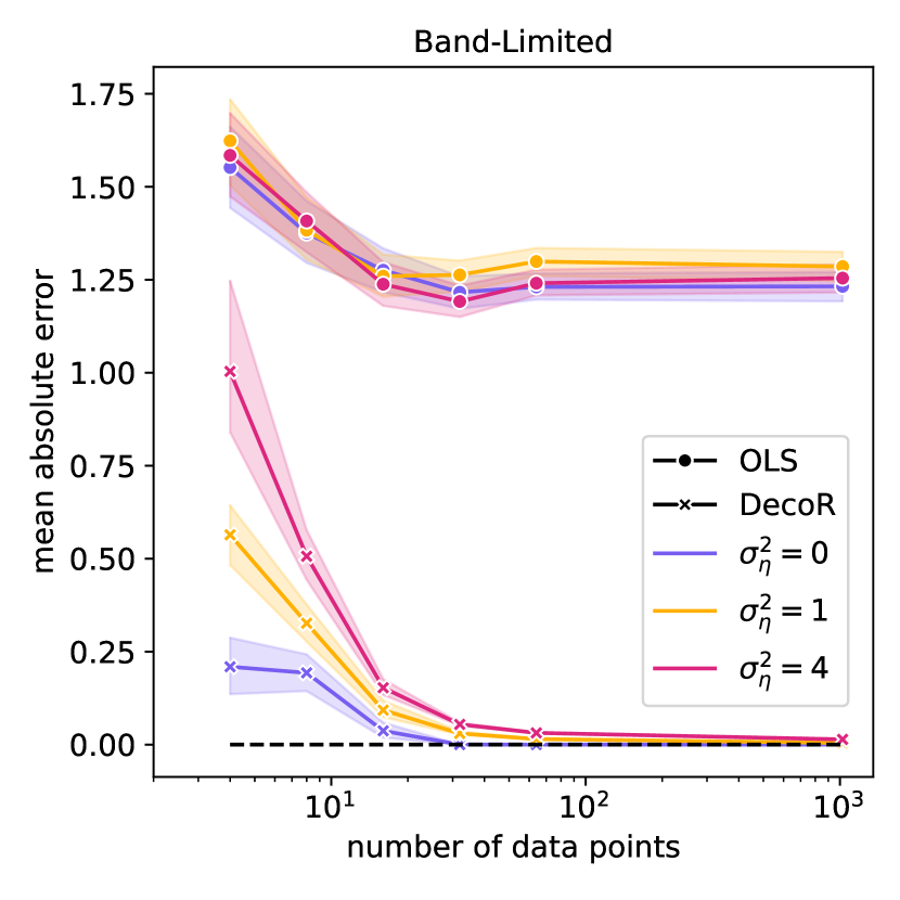
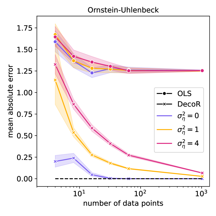
Figure 3: Synthetic experiment where $\epsilon_{x}$ and $U$ are generated by two independent band-limited processes (left) or two independent Ornstein-Uhlenbeck processes (right) and where we choose $\phi$ to be the cosine basis. For this experiment DecoR-Tor is used.

6 Summary and Future Work

In this work we have developed DecoR, an algorithm that estimates causal effects in the presence of unobserved confounders in time series data. We leverage sparsity in $L^{2}$ with respect to a known basis to derive conditions under which DecoR consistently estimates the true causal effect.

Looking ahead, we see several promising directions for future work. First, adapting our results to datasets where the data points are not observed in regular intervals. Similarly, extending our framework to include the asymptotics of longer observational time horizons, as opposed to shorter time intervals, would be interesting. Second, exploring scenarios where the effect of the hidden confounder has a linear and sparse effect on $X$, but is dense toward $Y$, may be relevant for practical applications. For such cases, similarly as before, we have

$$T_{k}^{\phi,n}(Y)=T_{k}^{\phi,n}(X)^{\top}\beta+T_{k}^{\phi,n}(U)+T_{k}^{\phi,n}(\eta).$$

However, in contrast to Setting 1, the hidden confounder does not disappear, that is, $(T_{k}^{\phi,n}(U))_{G^{c}}\neq 0$. Instead, assuming $X=\alpha U+\epsilon_{X}$ for some $\alpha\in\mathbb{R}^{d}$ and $\epsilon_{X}\perp\!\!\!\perp X$, one may be able to exploit that $(T_{k}^{\phi,n}(X))_{G_{n}^{c}}^{\top}(T_{k}^{\phi,n}(U))_{G_{n}^{c}}\to 0$. Lastly, it could be interesting to extend the results about the lower bound to other noise distributions such as the Gaussian distribution. We hypothesize that, in this case, our approach would be consistent under minor modifications. Third, another promising direction is to consider nonlinear causal effects. In this setting, one strategy could be to generalize the derived results to finite-dimensional feature transformations or to kernelize the approach.

Appendix A Visualization of DecoR

Figure 4 provides another visualization of the proposed procedure DecoR.

Figure 4: Visualization of DecoR (Section 2.1): in the time domain (left), the processes are confounded, so estimators based on least squares will generally be biased. Assuming that the confounding is sparse in the frequency domain (middle), we can apply robust regression methods to estimate the causal effect (right). We prove that DecoR is consistent under weak assumptions if the confounding is sparse; see Section 4.

Appendix B Comment on Setting 1

Setting 1 is more general than the additive structure may initially suggest. To see this, let $\tilde{X}=(\tilde{X}_{t})_{t\in[0,T]}$ be a stochastic process and let $\epsilon=(\epsilon_{t})_{t\in[0,T]}$ be any noise process; in particular, $\epsilon$ might depend on $\tilde{X}$. Assume that the stochastic process $\tilde{Y}=(\tilde{Y}_{t})_{t\in[0,T]}$ satisfies

$$\tilde{Y}_{t}\coloneqq\tilde{\beta}\tilde{X}_{t}+\epsilon_{t},$$ (11)

where $\tilde{\beta}\in\mathbb{R}^{d}$ denotes the total causal effect of $\tilde{X}_{t}$ on $\tilde{Y}_{t}$. Without loss of generality, there exist random vectors $\tilde{U}=\{\tilde{U}_{t}\}_{t\in[0,T]}$, an independent stochastic process $\tau=(\tau_{t})_{t\in[0,T]}$, and measurable function $(h_{t})_{t\in[0,T]}$ such that

$$\tilde{X}_{t} \coloneqq h_{t}(\tilde{U}_{t},\tau),$$

$$\tilde{Y}_{t} \coloneqq\tilde{\beta}\tilde{X}_{t}+\tilde{U}_{t}$$

and $\tilde{U}$ and $\tau$ are independent. This statement follows when defining $\tilde{U}_{t}:=\epsilon_{t}$ and choosing the equation $h_{t}$ and $\tau$ accordingly (see Peters et al., 2017, Proposition 4.1). In this structural causal model, $\tilde{\beta}$ is the causal effect from $\tilde{X}_{t}$ to $\tilde{Y}_{t}$. Since we allow for a degenerate noise process, Setting 1 thus includes (11) as a special case.

Appendix C Additional Definitions

Definition C.1 (Cosine basis).

Let $T\in\mathbb{R}_{>0}$ be a fixed constant. Define, for all $k\in\mathbb{N}$, the function $\phi_{k}:[0,T]\to\mathbb{R}$ by

$$x\mapsto\begin{cases}1&\text{if $x=0$ and}\\ \sqrt{2}\cos(x\pi(k+1/2))&\text{otherwise.}\end{cases}$$

We call $\phi\coloneqq(\phi_{k})_{k\in\mathbb{N}}$ the cosine basis.

By definition, the cosine basis is right-continuous and its discretization is also called the inverse DCT (Ahmed et al., 1974).

Definition C.2 (Haar basis (Haar, 1909)).

Let $T\in\mathbb{R}_{>0}$ be a fixed constant. Define the function $\phi^{\mathrm{H}}_{0}:[0,T]\to\mathbb{R}$ by

$$x\mapsto\begin{cases}1&\text{if $x\leq T/2$}\\ -1&\text{if $x>T/2$}.\end{cases}$$

Define, for all $k\in\mathbb{N}$, the function $\phi^{\mathrm{H}}_{k}:[0,T]\to\mathbb{R}$ by

$$x\mapsto 2^{-k/2}\phi^{\mathrm{H}}_{0}(2^{k}x).$$

We call $\phi\coloneqq(\phi_{k})_{k\in\mathbb{N}}$ the Haar basis.

By definition, the Haar basis is right-continuous.

Definition C.3 (Bachmann–Landau notation).

Let $f,g:\mathbb{N}\to\mathbb{R}$. We say $|f|$ is bounded from above by g asymptotically and write $f(n)\in\mathcal{O}(g(n))$ if

$$\limsup_{n\to\infty}\frac{f(n)}{g(n)}<\infty.$$

We say $f$ is bounded from below by g asymptotically and write $f(n)\in\Omega(g(n))$ if

$$\liminf_{n\to\infty}\frac{f(n)}{g(n)}>0.$$

Definition C.4.

Let $X_{1},X_{2},\ldots$ be a sequence of random variables and $g:\mathbb{N}\to\mathbb{R}$ a real-valued function. We say that with high probability it holds that

$$X_{n}\in\mathcal{O}(g(n))$$

if for all $\delta>0$ there exists a real-valued function $f_{\delta}:\mathbb{N}\to\mathbb{R}$ such that

$$\text{for all }n\in\mathbb{N}:\qquad\mathbb{P}\left[X_{n}\leq f_{\delta}(n)\right]\geq 1-\delta$$

and

$$f_{\delta}(n)\in\mathcal{O}(g(n)).$$

We define $X_{n}\in o(g(n))$ with high probability and $X_{n}\in\Omega(g(n))$ with high probability analogously.

Appendix D Proofs

D.1 Lemmas

Lemma D.1 (Theorem 6.3.2 of Vershynin (2018)).

Let $\mu$ be a sub-Gaussian distribution with zero mean and unit variance. There exists a constant $K>0$ such that for all $n\in\mathbb{N}$ the following holds: Let $\epsilon_{1},\dots,\epsilon_{n}$ be i.i.d distributed with respect to $\mu$ and define $\epsilon^{n}\coloneqq(\epsilon_{1},\dots,\epsilon_{n})$. Then for all $A\in\mathbb{R}^{m\times n}$ and $t\geq 0$ we have that

$$\mathbb{P}\left(\Big{|}\left\lVert A\epsilon^{n}\right\rVert_{2}-\left\lVert A\right\rVert_{\mathrm{F}}\Big{|}\geq t\right)\leq 2\exp\left(-\frac{t^{2}}{K\left\lVert A\right\rVert^{2}_{2}}\right).$$

D.2 Proof of Theorem 3.1

We first proof a result for general noise variables:

Theorem D.2.

Assume Setting 2 with $d=1$ and that $\mathrm{Inl}(\mathcal{U}_{n})\neq\emptyset$. Define for $S\in\mathcal{U}_{n}$ and for $U_{n}\in\mathrm{Inl}(\mathcal{U}_{n})$

$$\eta_{1}(S)\coloneqq\frac{|X_{S}^{\top}\epsilon_{S}|}{\left\lVert X_{S}\right\rVert_{2}^{2}}$$ (12)

and

$$\begin{split}\eta_{2}^{2}(S,U_{n})&\coloneqq\frac{1}{\left\lVert X_{S\setminus G_{n}}\right\rVert_{2}^{2}}\Bigg{(}\frac{|{S}|}{|U_{n}|}\left\lVert\epsilon_{U_{n}}\right\rVert_{2}^{2}-\left\lVert\epsilon_{S}\right\rVert_{2}^{2}-2\epsilon_{S}^{\top}o_{S}\\ &\quad+\frac{(X_{S}^{\top}\epsilon_{S})^{2}}{\left\lVert X_{S}\right\rVert_{2}^{2}}+2\frac{\left|X_{S}^{\top}\epsilon_{S}\right|\left|X_{S}^{\top}o_{S}\right|}{\left\lVert X_{S}\right\rVert_{2}^{2}}-\frac{|{S}|(X_{U_{n}}^{\top}\epsilon_{U_{n}})^{2}}{|U_{n}|\left\lVert X_{U_{n}}\right\rVert_{2}^{2}}\Bigg{)}.\end{split}$$ (13)

Then

$$\left|\hat{\beta}^{n}_{\texttt{BFS}}(\mathcal{U}_{n})-\beta\right|\leq\max_{S\in\mathcal{U}_{n}}\min_{U_{n}\in\mathrm{Inl}(\mathcal{U}_{n})}\left(\eta_{1}(S)+\eta_{2}(S,U_{n})\right).$$

Lemma D.3.

Assume Setting 2 with $d=1$. Let $S\in\mathcal{P}(\{1,\dots,n\})\setminus\{\emptyset\}$ and assume that $\left\lVert X_{S}\right\rVert_{2}>0$. The squared prediction error of the OLS estimator when using the data with indices $S$ is given by

$$\left\lVert\hat{\beta}_{\texttt{OLS}}^{S}X_{S}-Y_{S}\right\rVert_{2}^{2} =\left\lVert\epsilon_{S}\right\rVert_{2}^{2}+\left\lVert o_{S}\right\rVert_{2}^{2}+2\epsilon_{S}^{\top}o_{S}-\left(\frac{X_{S}^{\top}\epsilon_{S}}{\left\lVert X_{S}\right\rVert_{2}}+\frac{X_{S}^{\top}o_{S}}{\left\lVert X_{S}\right\rVert_{2}}\right)^{2}.$$

Proof.

It holds that

$$\left\lVert\hat{\beta}_{\texttt{OLS}}^{S}X_{S}-Y_{S}\right\rVert_{2}^{2} =\left\lVert\frac{X_{S}^{\top}(\epsilon_{S}+o_{S})X_{S}}{\left\lVert X_{S}\right\rVert_{2}^{2}}-\epsilon_{S}-o_{S}\right\rVert_{2}^{2}$$

$$=\left\lVert\epsilon_{S}+o_{S}\right\rVert_{2}^{2}-\left(\frac{X_{S}^{\top}}{\left\lVert X_{S}\right\rVert_{2}}(\epsilon_{S}+o_{S})\right)^{2}$$

$$=\left\lVert\epsilon_{S}\right\rVert_{2}^{2}+\left\lVert o_{S}\right\rVert_{2}^{2}+2\epsilon_{S}^{\top}o_{S}-\left(\frac{X_{S}^{\top}\epsilon_{S}}{\left\lVert X_{S}\right\rVert_{2}}+\frac{X_{S}^{\top}o_{S}}{\left\lVert X_{S}\right\rVert_{2}}\right)^{2}.$$

∎

We are now able to prove Theorem D.2. Let

$$S^{*}\in\operatorname*{arg\,min}_{S\in\mathcal{U}_{n}}\frac{1}{|S|}\left\lVert Y_{S}-X_{S}\hat{\beta}^{S}_{\texttt{OLS}}(X,Y)\right\rVert^{2}_{2}$$ (14)

be the set satisfying $\hat{\beta}^{S^{*}}_{\texttt{OLS}}=\hat{\beta}^{n}_{\texttt{BFS}}(\mathcal{U}_{n})$.

Proof of Theorem D.2.

Assume $X_{S^{*}}^{\top}X_{S^{*}}$ is invertible (otherwise the bound is void). By the definition of $S^{*}$ (see (14)),

$$\frac{1}{|S^{*}|}\left\lVert\hat{\beta}_{\texttt{OLS}}^{S^{*}}X_{S^{*}}-Y_{S^{*}}\right\rVert_{2}^{2}\leq\frac{1}{|U_{n}|}\left\lVert\hat{\beta}_{\texttt{OLS}}^{U_{n}}X_{U_{n}}-Y_{U_{n}}\right\rVert^{2}_{2}.$$

This implies by Lemma D.3 that

$$\frac{1}{|S^{*}|}\left(\left\lVert\epsilon_{S^{*}}\right\rVert_{2}^{2}+\left\lVert o_{S^{*}}\right\rVert_{2}^{2}+2\epsilon_{S^{*}}^{\top}o_{S^{*}}-\left(\frac{X_{S^{*}}^{\top}\epsilon_{S^{*}}}{\left\lVert X_{S^{*}}\right\rVert_{2}}+\frac{X_{S^{*}}^{\top}o_{S^{*}}}{\left\lVert X_{S^{*}}\right\rVert_{2}}\right)^{2}\right) =\frac{1}{|S^{*}|}\left\lVert\hat{\beta}_{\texttt{OLS}}^{S^{*}}X_{S^{*}}-Y_{S^{*}}\right\rVert_{2}^{2}$$

$$\leq\frac{1}{|U_{n}|}\left\lVert\hat{\beta}_{\texttt{OLS}}^{U_{n}}X_{U_{n}}-Y_{U_{n}}\right\rVert^{2}_{2}$$

$$\leq\frac{\left\lVert\epsilon_{U_{n}}\right\rVert_{2}^{2}}{|U_{n}|}-\frac{(X_{U_{n}}^{\top}\epsilon_{U_{n}})^{2}}{|U_{n}|\left\lVert X_{U_{n}}\right\rVert_{2}^{2}},$$

using $o_{U_{n}}=0$ in the last inequality. Rearranging gives

$$\begin{split}\left\lVert o_{S^{*}}\right\rVert^{2}_{2}-\left(\frac{X_{S^{*}}^{\top}o_{S^{*}}}{\left\lVert X_{S^{*}}\right\rVert_{2}}\right)^{2}&\leq\frac{|{S^{*}}|}{|U_{n}|}\left\lVert\epsilon_{U_{n}}\right\rVert_{2}^{2}-\left\lVert\epsilon_{S^{*}}\right\rVert_{2}^{2}-2\epsilon_{S^{*}}^{\top}o_{S^{*}}+\\ &\quad\frac{(X_{S^{*}}^{\top}\epsilon_{S^{*}})^{2}}{\left\lVert X_{S^{*}}\right\rVert_{2}^{2}}+2\frac{\left|X_{S^{*}}^{\top}\epsilon_{S^{*}}\right|\left|X_{S^{*}}^{\top}o_{S^{*}}\right|}{\left\lVert X_{S^{*}}\right\rVert_{2}^{2}}-\frac{|{S^{*}}|(X_{U_{n}}^{\top}\epsilon_{U_{n}})^{2}}{|U_{n}|\left\lVert X_{U_{n}}\right\rVert_{2}^{2}}\\ &=\eta_{2}^{2}(S^{*},U_{n})\left\lVert X_{{S^{*}}\setminus G_{n}}\right\rVert_{2}^{2}.\end{split}$$ (15)

By Cauchy-Schwarz and the fact that $o_{i}=0$ for all $i\notin G_{n}$ we have

$$\begin{split}\left\lVert o_{S^{*}}\right\rVert^{2}_{2}\frac{\left\lVert X_{S^{*}\setminus G_{n}}\right\rVert^{2}_{2}}{\left\lVert X_{S^{*}}\right\rVert^{2}_{2}}&=\left\lVert o_{S^{*}}\right\rVert^{2}_{2}\left(1-\frac{\left\lVert X_{S^{*}\cap G_{n}}\right\rVert^{2}_{2}}{\left\lVert X_{S^{*}}\right\rVert^{2}_{2}}\right)\\ &\leq\left\lVert o_{S^{*}}\right\rVert^{2}_{2}\left(1-\frac{(X_{S^{*}\cap G_{n}}^{\top}\;o_{S^{*}\cap G_{n}})^{2}}{\left\lVert X_{S^{*}}\right\rVert^{2}_{2}\left\lVert o_{S^{*}\cap G_{n}}\right\rVert^{2}_{2}}\right)\\ &=\left\lVert o_{S^{*}}\right\rVert^{2}_{2}\left(1-\frac{(X_{S^{*}}^{\top}o_{S^{*}})^{2}}{\left\lVert X_{S^{*}}\right\rVert^{2}_{2}\left\lVert o_{S^{*}}\right\rVert^{2}_{2}}\right)\\ &=\left\lVert o_{S^{*}}\right\rVert^{2}_{2}-\left(\frac{X_{S^{*}}^{\top}o_{S^{*}}}{\left\lVert X_{S^{*}}\right\rVert_{2}}\right)^{2}.\end{split}$$ (16)

Combining (15) and (16) yields

$$\frac{\left\lVert o_{S^{*}}\right\rVert_{2}}{\left\lVert X_{S^{*}}\right\rVert_{2}}\leq\eta_{2}(S^{*},U_{n}).$$

By (14)

$$\left|\hat{\beta}^{n}_{\texttt{BFS}}(\mathcal{U}_{n})-\beta\right| \leq\frac{|X_{S^{*}}^{\top}\epsilon_{S^{*}}|}{\left\lVert X_{S^{*}}\right\rVert_{2}^{2}}+\frac{|X_{S^{*}}^{\top}o_{S^{*}}|}{\left\lVert X_{S^{*}}\right\rVert_{2}^{2}}$$

$$\leq\frac{|X_{S^{*}}^{\top}\epsilon_{S^{*}}|}{\left\lVert X_{S^{*}}\right\rVert_{2}^{2}}+\frac{\left\lVert o_{S^{*}}\right\rVert_{2}}{\left\lVert X_{S^{*}}\right\rVert_{2}}$$

$$\leq\eta_{1}(S^{*})+\eta_{2}(S^{*},U_{n}).$$

Since this holds for all $U_{n}\in\mathrm{Inl}(\mathcal{U}_{n})$, we have

$$\left|\hat{\beta}^{n}_{\texttt{BFS}}(\mathcal{U}_{n})-\beta\right|\leq\min_{U_{n}\in\mathrm{Inl}(\mathcal{U}_{n})}\left(\eta_{1}(S^{*})+\eta_{2}(S^{*},U_{n})\right)\leq\max_{S\in\mathcal{U}_{n}}\min_{U_{n}\in\mathrm{Inl}(\mathcal{U}_{n})}\left(\eta_{1}(S)+\eta_{2}(S,U_{n})\right).$$

∎

Proof of Theorem 3.1.

Let $U_{n}\in\mathrm{Inl}(\mathcal{U}_{n})$. By the proof of Theorem D.2, specifically (15) and (16), we have that

$$\left\lVert o_{S^{*}}\right\rVert^{2}_{2}\frac{\left\lVert X_{S^{*}\setminus G_{n}}\right\rVert^{2}_{2}}{\left\lVert X_{S^{*}}\right\rVert^{2}_{2}} \leq\frac{|{S^{*}}|}{|U_{n}|}\left\lVert\epsilon_{U_{n}}\right\rVert_{2}^{2}-\left\lVert\epsilon_{S^{*}}\right\rVert_{2}^{2}-2\epsilon_{S^{*}}^{\top}o_{S^{*}}$$

$$\quad+\frac{(X_{S^{*}}^{\top}\epsilon_{S^{*}})^{2}}{\left\lVert X_{S^{*}}\right\rVert_{2}^{2}}+2\frac{\left|X_{S^{*}}^{\top}\epsilon_{S^{*}}\right|\left|X_{S^{*}}^{\top}o_{S^{*}}\right|}{\left\lVert X_{S^{*}}\right\rVert_{2}^{2}}-\frac{|{S^{*}}|(X_{U_{n}}^{\top}\epsilon_{U_{n}})^{2}}{|U_{n}|\left\lVert X_{U_{n}}\right\rVert_{2}^{2}}.$$ (17)

We bound the terms on the RHS. It holds that for all $S\in\mathcal{P}(\{1,\dots,n\})\setminus\{\emptyset\}$

$$X_{S}^{\top}\epsilon_{S}\sim\mathcal{N}\left(0,\sigma^{2}\left\lVert X_{S}\right\rVert_{2}^{2}\right)$$

and $$o_{S}^{\top}\epsilon_{S}\sim\mathcal{N}\left(0,\sigma^{2}\left\lVert o_{S}\right\rVert_{2}^{2}\right).$$

Therefore, by the Gaussian concentration inequality and the union bound,

$$\mathbb{P}\left[\forall S\in\mathcal{U}_{n},|X_{S}^{\top}\epsilon_{S}|\leq\sigma{\left\lVert X_{S}\right\rVert_{2}}\sqrt{2\log(2|\mathcal{U}_{n}|/\delta)}\right]\geq 1-\delta$$ (18)

and

$$\mathbb{P}\left[\forall S\in\mathcal{U}_{n},|o_{S}^{\top}\epsilon_{S}|\leq\sigma{\left\lVert o_{S}\right\rVert_{2}}\sqrt{2\log(2|\mathcal{U}_{n}|/\delta)}\right]\geq 1-\delta.$$

By Lemma D.1 there exists $K>0$ such that for all $t\geq 0$ we have

$$\mathbb{P}\left[\forall S\in\mathcal{U}_{n},\left|\left\lVert\epsilon_{S}\right\rVert_{2}-\sigma\sqrt{|S|}\right|\geq t\right]\leq 2|\mathcal{U}_{n}|\exp\left(-\frac{t^{2}}{K\sigma^{2}}\right)$$

and therefore

$$\mathbb{P}\left[\forall S\in\mathcal{U}_{n},\left|\left\lVert\epsilon_{S}\right\rVert_{2}-\sigma\sqrt{|S|}\right|\leq\sigma\sqrt{K\log(2|\mathcal{U}_{n}|/\delta)}\right]\geq 1-\delta.$$

This yields with probability at least $1-\delta$ jointly for all $S\in\mathcal{U}_{n}$

$$\frac{|S|}{|U_{n}|}\left\lVert\epsilon_{U_{n}}\right\rVert_{2}^{2}-\left\lVert\epsilon_{S}\right\rVert_{2}^{2} \leq\frac{|S|}{{|U_{n}|}}\left(\sigma\sqrt{|U_{n}|}+\sigma\sqrt{K\log(2|\mathcal{U}_{n}|/\delta)}\right)^{2}-\left(\sigma\sqrt{|S|}-\sigma\sqrt{K\log(2|\mathcal{U}_{n}|/\delta)}\right)^{2}$$

$$=\alpha_{1}(S,U_{n},\delta).$$

Using the three inequalities above (and Cauchy-Schwarz for the term $|X_{S^{*}}^{\top}o_{S^{*}}|$) to bound the terms of the RHS of (D.2), we therefore have with probability at least $1-3\delta$

$$\frac{\left\lVert o_{S^{*}}\right\rVert^{2}_{2}}{\left\lVert X_{S^{*}}\right\rVert^{2}_{2}} \leq\frac{\alpha_{1}(S^{*},U_{n},\delta)}{\left\lVert X_{{S^{*}}\setminus G_{n}}\right\rVert^{2}_{2}}+4\frac{\sigma\left\lVert o_{S^{*}}\right\rVert_{2}\sqrt{2\log(2|\mathcal{U}_{n}|/\delta)}}{\left\lVert X_{{S^{*}}\setminus G_{n}}\right\rVert_{2}^{2}}+\left(\frac{\sigma\sqrt{2\log(2|\mathcal{U}_{n}|/\delta)}}{\left\lVert X_{{S^{*}}\setminus G_{n}}\right\rVert_{2}}\right)^{2}.$$

Solving the quadratic equation with respect to $\left\lVert o_{S^{*}}\right\rVert_{2}$ yields

$$\frac{\left\lVert o_{S^{*}}\right\rVert_{2}}{\left\lVert X_{S^{*}}\right\rVert_{2}} \leq\frac{4\sigma\left\lVert X_{{S^{*}}}\right\rVert_{2}\sqrt{2\log(2|\mathcal{U}_{n}|/\delta)}}{\left\lVert X_{{S^{*}}\setminus G_{n}}\right\rVert_{2}^{2}}+\frac{\sqrt{\alpha_{1}(S^{*},U_{n},\delta)}}{\left\lVert X_{{S^{*}}\setminus G_{n}}\right\rVert_{2}}+\frac{\sigma\sqrt{2\log(2|\mathcal{U}_{n}|/\delta)}}{\left\lVert X_{{S^{*}}\setminus G_{n}}\right\rVert_{2}}$$

$$=\alpha(S^{*},U_{n},\delta)$$ (19)

As shown in the proof of Theorem D.2, we have

$$\left|\hat{\beta}^{n}_{\texttt{BFS}}(\mathcal{U}_{n})-\beta\right|\leq\frac{|X_{S^{*}}^{\top}\epsilon_{S^{*}}|}{\left\lVert X_{S^{*}}\right\rVert_{2}^{2}}+\frac{\left\lVert o_{S^{*}}\right\rVert_{2}}{\left\lVert X_{S^{*}}\right\rVert_{2}}.$$

Using (18) and (19), we thus obtain with probability at least $1-3\delta$

$$\left|\hat{\beta}^{n}_{\texttt{BFS}}(\mathcal{U}_{n})-\beta\right|\leq\min_{U_{n}\in\mathrm{Inl}(\mathcal{U}_{n})}\left\{\alpha(S^{*},U_{n},\delta)+\frac{\sigma\sqrt{2\log(2|\mathcal{U}_{n}|/\delta)}}{\left\lVert X_{S^{*}}\right\rVert_{2}}\right\}.$$

and therefore the desired result. ∎

D.3 Proof of Lemma 3.2

The number of distinct sets $S$ that Torrent can output is trivially bounded by $\binom{n}{\lfloor a\rfloor}$. Furthermore, it holds that

$$\left\lVert X_{S_{t+1}}(\beta-\hat{\beta}^{t+1}_{\texttt{Tor}})+\epsilon_{S_{t+1}}+o_{S_{t+1}}\right\rVert_{2} \leq\left\lVert X_{S_{t+1}}(\beta-\hat{\beta}^{t}_{\texttt{Tor}})+\epsilon_{S_{t+1}}+o_{S_{t+1}}\right\rVert_{2}$$

$$\leq\left\lVert X_{S_{t}}(\beta-\hat{\beta}^{t}_{\texttt{Tor}})+\epsilon_{S_{t}}+o_{S_{t}}\right\rVert_{2}.$$

The first inequality holds because $\hat{\beta}_{\texttt{Tor}}^{t+1}$ is the least squares estimate for data $X_{S_{t+1}}$, while the second holds because of the hard thresholding step. Furthermore, this implies that Torrent converges after finitely many steps.

D.4 Proof of Theorem 3.3

Assume that $X_{S_{t}}^{\top}X_{S_{t}}$ is invertible (otherwise, the bound is void). We begin by observing that the optimality of the model $\hat{\beta}^{t}_{\texttt{Tor}}$ on the active set $S_{t}$ ensures

$$\begin{split}\left\lVert\hat{\beta}^{t}_{\texttt{Tor}}-\beta\right\rVert_{2}&=\left\lVert\left(X_{S_{t}}^{\top}X_{S_{t}}\right)^{-1}\left(X_{S_{t}}^{\top}\epsilon_{S_{t}}+X_{S_{t}}^{\top}o_{S_{t}}\right)\right\rVert_{2}\\ &\leq\left\lVert\left(X_{S_{t}}^{\top}X_{S_{t}}\right)^{-1}X_{S_{t}}^{\top}\epsilon_{S_{t}}\right\rVert_{2}+\left\lVert\left(X_{S_{t}}^{\top}X_{S_{t}}\right)^{-1}X_{S_{t}}^{\top}\right\rVert_{2}\left\lVert o_{S_{t}}\right\rVert_{2}.\end{split}$$ (20)

The hard thresholding step guarantees that

$$\begin{split}\left\|X_{S_{t+1}}\left(\beta-\hat{\beta}^{t}_{\texttt{Tor}}\right)+\epsilon_{S_{t+1}}+o_{S_{t+1}}\right\|_{2}^{2}&=\left\|Y_{S_{t+1}}-X_{S_{t+1}}\hat{\beta}^{t}_{\texttt{Tor}}\right\|_{2}^{2}\\ &\leq\left\|Y_{G_{n}^{\mathsf{c}}}-X_{G_{n}^{\mathsf{c}}}\hat{\beta}^{t}_{\texttt{Tor}}\right\|^{2}_{2}\\ &=\left\|X_{G_{n}^{\mathsf{c}}}\left(\beta-\hat{\beta}^{t}_{\texttt{Tor}}\right)+\epsilon_{G_{n}^{\mathsf{c}}}\right\|_{2}^{2}.\end{split}$$ (21)

Let $H_{t+1}\coloneqq S_{t+1}\backslash G_{n}^{\mathsf{c}}$ and $M_{t+1}\coloneqq G_{n}^{\mathsf{c}}\backslash S_{t+1}$. It then follows from (21)

$$\left\|X_{H_{t+1}}\left(\beta-\hat{\beta}^{t}_{\texttt{Tor}}\right)+\epsilon_{H_{t+1}}+o_{H_{t+1}}\right\|_{2}\leq\left\|X_{M_{t+1}}\left(\beta-\hat{\beta}^{t}_{\texttt{Tor}}\right)+\epsilon_{M_{t+1}}\right\|_{2}.$$

Let $V_{t+1}\coloneqq H_{t+1}\cup M_{t+1}$ then $V_{t+1}=(S_{t+1}\cup G_{n}^{\mathsf{c}})\setminus(G_{n}^{\mathsf{c}}\cap S_{t+1})=V(S_{t})$. An application of the triangle inequality and the fact that $\left\|o_{H_{t+1}}\right\|_{2}=\left\|o_{S_{t+1}}\right\|_{2}$ gives us

$$\begin{split}\left\|o_{S_{t+1}}\right\|_{2}&\leq\left\|X_{M_{t+1}}\left(\beta-\hat{\beta}^{t}_{\texttt{Tor}}\right)\right\|_{2}+\left\|X_{H_{t+1}}\left(\beta-\hat{\beta}^{t}_{\texttt{Tor}}\right)\right\|_{2}+\left\|\epsilon_{H_{t+1}}\right\|_{2}+\left\|\epsilon_{M_{t+1}}\right\|_{2}\\ &\leq\sqrt{2}\left\lVert X_{V_{t+1}}\right\rVert_{2}\left\|\beta-\hat{\beta}^{t}_{\texttt{Tor}}\right\|_{2}+\sqrt{2}\|\epsilon_{V_{t+1}}\|_{2}\\ &\leq\sqrt{2}\left\lVert X_{V_{t+1}}\right\rVert_{2}\left(\left\lVert\left(X_{S_{t}}^{\top}X_{S_{t}}\right)^{-1}X_{S_{t}}^{\top}\epsilon_{S_{t}}\right\rVert_{2}+\left\lVert\left(X_{S_{t}}^{\top}X_{S_{t}}\right)^{-1}X_{S_{t}}^{\top}\right\rVert_{2}\left\lVert o_{S_{t}}\right\rVert_{2}\right)\\ &\quad+\sqrt{2}\|\epsilon_{V_{t+1}}\|_{2}\\ &=\sqrt{2}\left\lVert X_{V_{t+1}}\right\rVert_{2}\left\lVert\left(X_{S_{t}}^{\top}X_{S_{t}}\right)^{-1}X_{S_{t}}^{\top}\right\rVert_{2}\left\lVert o_{S_{t}}\right\rVert_{2}+\sqrt{2}\left\lVert X_{V_{t+1}}\right\rVert_{2}\left\lVert\left(X_{S_{t}}^{\top}X_{S_{t}}\right)^{-1}X_{S_{t}}^{\top}\epsilon_{S_{t}}\right\rVert_{2}\\ &\quad+\sqrt{2}\|\epsilon_{V_{t+1}}\|_{2}.\end{split}$$ (22)

Here the second inequality follows since for all $x\in\mathbb{R}^{d}$ we have $\left\lVert x\right\rVert_{1}\leq\sqrt{d}\left\lVert x\right\rVert_{2}$. Let $t$ be the iteration where Torrent has converged (see Lemma 3.2). We prove that we can assume that either $S_{t}=S_{t+1}$ or $S_{t+1}=S_{t+2}$ hold. First, assume that $\hat{\beta}^{t+1}_{\texttt{Tor}}=\hat{\beta}^{t}_{\texttt{Tor}}$. Then, by Algorithm 3 we have $S_{t+1}=S_{t+2}$. Next, assume $\hat{\beta}^{t+1}_{\texttt{Tor}}\neq\hat{\beta}^{t}_{\texttt{Tor}}$. If $X_{S_{t+1}}^{T}X_{S_{t+1}}$ is not invertible, the bound is void and there is nothing to show. If $X_{S_{t+1}}^{T}X_{S_{t+1}}$ is invertible, then $\hat{\beta}^{t+1}_{\texttt{Tor}}$ is the unique minima and the algorithm did not stop, which is a contraction to the assumption that $S_{t}$ is the output of Torrent. Without loss of generality, we can therefore assume that $S_{t}=S_{t+1}$.

Since for all $A\in\mathbb{R}^{n\times d}$ we have $\left\lVert A\right\rVert_{2}=\sqrt{\lambda_{\mathrm{max}}(A^{\top}A)}=\sqrt{\lambda_{\mathrm{max}}(AA^{\top})}=(\lambda_{\mathrm{min}}((AA^{\top})^{-1}))^{-1/2}$ and by assumption we have

$$\eta=\max_{S\subseteq\{1,\dots,n\}\text{ s.t. }|S|=a_{n}}\frac{\left\lVert X_{V(S)}\right\rVert_{2}}{\sqrt{\lambda_{\mathrm{min}}\left(X_{S}^{T}X_{S}\right)}}=\max_{S\subseteq\{1,\dots,n\}\text{ s.t. }|S|=a_{n}}\left\lVert X_{V(S)}\right\rVert_{2}\left\lVert\left(X_{S}^{\top}X_{S}\right)^{-1}X_{S}^{\top}\right\rVert_{2}<\frac{1}{\sqrt{2}}.$$

Together with $S_{t}=S_{t+1}$ this yields

$$\left\|o_{S_{t}}\right\|_{2}\leq\sqrt{2}\eta\left\lVert o_{S_{t}}\right\rVert_{2}+2\left\lVert X_{V_{t}}\right\rVert_{2}\left\lVert\left(X_{S_{t}}^{\top}X_{S_{t}}\right)^{-1}X_{S_{t}}^{\top}\epsilon_{S_{t}}\right\rVert_{2}+\sqrt{2}\|\epsilon_{V_{t}}\|_{2}$$

and therefore

$$\left\|o_{S_{t}}\right\|_{2}\leq\frac{2\left\lVert X_{V_{t}}\right\rVert_{2}\left\lVert\left(X_{S_{t}}^{\top}X_{S_{t}}\right)^{-1}X_{S_{t}}^{\top}\epsilon_{S_{t}}\right\rVert_{2}+\sqrt{2}\|\epsilon_{V_{t}}\|_{2}}{1-\sqrt{2}\eta}.$$

Together with (20) this yields the following result.

$$\left\lVert\hat{\beta}^{n,a_{n}}_{\texttt{Tor}}-\beta\right\rVert_{2}=\left\lVert\hat{\beta}^{t}_{\texttt{Tor}}-\beta\right\rVert_{2} \leq\left\lVert\left(X_{S_{t}}^{\top}X_{S_{t}}\right)^{-1}X_{S_{t}}^{\top}\epsilon_{S_{t}}\right\rVert_{2}$$

$$\quad+\left\lVert\left(X_{S_{t}}^{\top}X_{S_{t}}\right)^{-1}X_{S_{t}}^{\top}\right\rVert_{2}\frac{2\left\lVert X_{V_{t}}\right\rVert_{2}\left\lVert\left(X_{S_{t}}^{\top}X_{S_{t}}\right)^{-1}X_{S_{t}}^{\top}\epsilon_{S_{t}}\right\rVert_{2}+\sqrt{2}\|\epsilon_{V_{t}}\|_{2}}{1-\sqrt{2}\eta}.$$

D.5 Proof of Corollary 3.4

We trivially have $|(S_{t}\cup G_{n}^{\mathsf{c}})|\leq n$ and, since $|S_{t}|,|G_{n}^{\mathsf{c}}|\geq n-c_{n}$, we also have $|(G_{n}^{\mathsf{c}}\cap S_{t})|\geq n-2c_{n}$. Therefore,

$$|V(S_{t})|\leq 2c_{n}.$$

Since $|\{S\subseteq\{1,\dots,n\}\text{ s.t. }|S|=a_{n}\}|=\binom{n}{a_{n}}=\binom{n}{c_{n}}\leq(en/c_{n})^{c_{n}}$ and by Lemma D.1 and the union bound (see the proof of Theorem 3.1 for a similar argument), there exists $K>0$ such that with probability at least $1-\delta$ for all $t\in\mathbb{N}$ that

$$\left\lVert\epsilon_{V(S_{t})}\right\rVert_{2}\leq\sigma\sqrt{2c_{n}}\left(1+\sqrt{K\log(2en/c_{n}\delta)}\right).$$

With similar arguments and noting that $\left\lVert(X_{S_{t}}^{\top}X_{S_{t}})^{-1}X_{S_{t}}^{\top}\right\rVert_{\mathrm{F}}\leq\sqrt{d}\left\lVert(X_{S_{t}}^{\top}X_{S_{t}})^{-1}X_{S_{t}}^{\top}\right\rVert_{2}$ we have with probability at least $1-\delta$ for all $t\in\mathbb{N}$

$$\left\lVert\left(X_{S_{t}}^{\top}X_{S_{t}}\right)^{-1}X_{S_{t}}^{\top}\epsilon_{S_{t}}\right\rVert_{2}\leq\sigma\left\lVert\left(X_{S_{t}}^{\top}X_{S_{t}}\right)^{-1}X_{S_{t}}^{\top}\right\rVert_{2}\left(\sqrt{d}+\sqrt{2c_{n}K\log(2en/c_{n}\delta)}\right).$$

By Theorem 3.3 and the fact that $\left\lVert\left(X_{S_{t}}^{\top}X_{S_{t}}\right)^{-1}X_{S_{t}}^{\top}\right\rVert_{2}=\left(\lambda_{\mathrm{min}}\left(X_{S_{t}}^{T}X_{S_{t}}\right)\right)^{-1/2}$ we have

$$\left\lVert\hat{\beta}^{n,a_{n}}_{\texttt{Tor}}-\beta\right\rVert_{2} \leq\frac{\sigma}{\lambda_{a_{n}}(X)}\left(1+\frac{\sqrt{2}}{1-\sqrt{2}\eta}\right)\left(\sqrt{d}+\sqrt{2c_{n}K\log(2en/c_{n}\delta)}\right)+\frac{2\sigma\sqrt{c_{n}}\left(1+\sqrt{K\log(2en/c_{n}\delta)}\right)}{\lambda_{a_{n}}(X)(1-\sqrt{2}\eta)}.$$

This yields the first result. If the rows of $X$ are i.i.d. standard Gaussian random vectors, we have $\lambda_{a_{n}}(X)\in\Omega(\sqrt{n})$ (see Bhatia et al. (2015, Theorem 15)). This yields the second statement.

D.6 Proof of Theorem 4.1 and Theorem 4.2

Lemma D.4.

Assume the setup of Section 4, let $c_{n}$ be a sequence satisfying, for all $n$, $|G_{n}|\leq c_{n}$ and define the $\mathcal{U}_{n}$ as in Theorem 4.1 and let Assumption 2 be satisfied. Then, the following three statements hold.

1. $|\mathcal{U}_{n}|\leq\left(\frac{en}{c_{n}}\right)^{c_{n}}$,

2. for all $n\in\mathbb{N}$ the $n$ components of $\eta^{n}_{\phi}$ are i.i.d. centered Gaussian random variables with variance $\bar{\sigma}^{2}=\sigma_{\eta}^{2}/n$,

3. for all $\delta>0$ there exists $c^{\prime}>0$ and $\bar{n}\in\mathbb{N}$ such that for all $n\geq\bar{n}$ it holds that

   $$\mathbb{P}\left[\min_{S\in\mathcal{U}_{n}}\sqrt{\lambda_{\mathrm{min}}\left((X^{n}_{\phi})_{S\setminus G_{n}}^{T}(X^{n}_{\phi})_{S\setminus G_{n}}\right)}\geq c^{\prime}\right]\geq 1-\delta.$$

Proof.

Since $\{T_{k}^{\phi,n}(\eta)\}_{k\leq n}$ are linear combinations of independent centered Gaussians, they are jointly Gaussian with mean zero. By Assumption 2 (i) it holds that

$$\mathbb{E}\left[(\eta^{n}_{\phi})_{k}(\eta^{n}_{\phi})_{l}\right]=\mathbb{E}\left[T_{k}^{\phi,n}(\eta)T_{l}^{\phi,n}(\eta)\right] =\frac{1}{n^{2}}\sum_{i,j=1}^{n}\phi_{k}(Ti/n)\phi_{l}(Tj/n)\mathbb{E}[\eta_{Ti/n}\eta_{Tj/n}]$$

$$=\frac{\sigma_{\eta}^{2}}{n}\mathbbm{1}\{k=l\}.$$

This proves (ii). Furthermore, it holds by Sterling’s inequality that

$$|\mathcal{U}_{n}| =\binom{n}{c_{n}}\leq\left(\frac{en}{c_{n}}\right)^{c_{n}}.$$

This proves (i). We now prove (iii). Since for all $S\in\mathcal{U}_{n}$ we have $|S|=n-c_{n}$ and $|G_{n}|\leq c_{n}$ it holds that for all $S\in\mathcal{U}_{n}$ that $|S\setminus G_{n}|\geq n-2c_{n}$. Now, consider $\bar{n}$ from Assumption 2 (ii) and an arbitrary $n\geq\bar{n}$. Let $S^{\prime}_{n}$ be the set from Assumption 2 (ii). Then $|S\setminus G_{n}|\geq n-2c_{n}$ implies $|(S\setminus G_{n})\cap S^{\prime}_{n}|\geq d$. Therefore, we can choose an $S^{\prime\prime}\subseteq(S\setminus G_{n})\cap S^{\prime}_{n}$ with $|S^{\prime\prime}|=d$. By Assumption 2 (ii) we then have with probability at least $1-\delta$

$$\min_{S\in\mathcal{U}_{n}}\sqrt{\lambda_{\mathrm{min}}\left((X^{n}_{\phi})_{S^{\prime\prime}}^{T}(X^{n}_{\phi})_{S^{\prime\prime}}\right)}\geq c^{\prime}.$$

Since $\lambda_{\mathrm{min}}$ is superadditive for positive semi-definite matrices, with probability at least $1-\delta$,

$$\min_{S\in\mathcal{U}_{n}}\sqrt{\lambda_{\mathrm{min}}\left((X^{n}_{\phi})_{S\setminus G_{n}}^{T}(X^{n}_{\phi})_{S\setminus G_{n}}\right)}\geq c^{\prime}.$$

∎

Proof of Theorem 4.1.

We want to apply Theorem 3.1. Since for all $n\in\mathbb{N}$ and $j,i\leq T$ it holds that $\frac{1}{n}\sum_{l=1}^{n}\phi_{l}(Tj/n)\phi_{l}(Ti/n)=\mathbbm{1}{\{i=j\}}$ (by assumption) we have that

$$\begin{split}\left\lVert X^{n}_{\phi}\right\rVert^{2}_{2}&=\sum_{l=1}^{n}\frac{1}{n^{2}}\sum_{i,j=1}^{n}X_{iT/n}X_{jT/n}\phi_{l}(Tj/n)\phi_{l}(Ti/n)\\ &=\frac{1}{n}\sum_{j=1}^{n}X_{jT/n}^{2}\end{split}$$ (23)

Since $\sup_{t\in[0,T]}\mathbb{E}[X_{t}^{2}]<\infty$ there exists $\bar{c}>0$ such that for all $n\in\mathbb{N}$

$$\mathbb{E}\left[\left\lVert X^{n}_{\phi}\right\rVert^{2}_{2}\right]=\mathbb{E}\left[\frac{1}{n}\sum_{k=1}^{n}X_{kT/n}^{2}\right]\leq\bar{c}<\infty.$$

By Markov’s inequality we have for all $\delta>0$ and for all $n\in\mathbb{N}$ that

$$\mathbb{P}\left[\left\lVert X^{n}_{\phi}\right\rVert^{2}_{2}\leq\bar{c}/\delta\right]\geq 1-\delta,$$ (24)

By (24) and Lemma D.4 (iii) for all $\delta>0$ there exist $v_{1},v_{2}>0$ and $\bar{n}$ such that or all $n\geq\bar{n}$, with probability at least $1-\delta$, for all $S\in\mathcal{U}_{n}$, we have $||(X^{n}_{\phi})_{S\setminus G_{n}}||_{2}>v_{1}$ and $||(X^{n}_{\phi})_{S}||_{2}<v_{2}$. By definition of $\mathcal{U}_{n}$ we have that for all $S\in\mathcal{U}_{n}$ and all $U_{n}\in\mathrm{Inl}(\mathcal{U}_{n})$ it holds that $|S|=|U_{n}|=n-c_{n}$ and therefore $\alpha_{1}(S,U_{n},\delta)\leq 4\sigma^{2}\sqrt{n}\sqrt{2\log(2|\mathcal{U}_{n}|/\delta)}$. Property (i) and Property (ii) of Lemma D.4 then yield the claim by Theorem 3.1. ∎

Proof of Theorem 4.2.

Equation (10) implies that for large $n$ with high probability we have

$$\eta\coloneqq\max_{S\subseteq\{1,\dots,n\}\text{ s.t. }|S|=n-c_{n}}\frac{\left\lVert(X^{n}_{\phi})_{V(S)}\right\rVert_{2}}{\sqrt{\lambda_{\mathrm{min}}\left((X^{n}_{\phi})_{S}^{T}(X^{n}_{\phi})_{S}\right)}}\leq 1/\sqrt{2}$$

and by (iii) we know that for large $n$ we have with high probability that for all for all $S$ with $|S|=n-c_{n}$ the value of $\sqrt{\lambda_{\mathrm{min}}\left((X^{n}_{\phi})_{S}^{T}(X^{n}_{\phi})_{S}\right)}$ is lower bounded. This yields the desired result by Corollary 3.4. ∎

D.7 Proof of Proposition 4.3

It holds that

$$\hat{\beta}^{\phi,n}_{\texttt{OLS}}-\beta=\frac{(X^{n}_{\phi})^{\top}\eta^{n}_{\phi}}{\left\lVert X^{n}_{\phi}\right\rVert_{2}^{2}}+\frac{(X^{n}_{\phi})^{\top}o^{n}_{\phi}}{\left\lVert X^{n}_{\phi}\right\rVert_{2}^{2}}.$$

By Lemma D.4 (ii) the first term vanishes in probability. The second term, however, is non-vanishing in many cases, for example, when $U$ is a band-limited process and $X_{t}=U_{t}+\hat{\epsilon}_{t}$ for all $t\in[0,T]$, where $\hat{\epsilon}$ is a band-limited process independent of $U$.

Appendix E Additional Results

E.1 Consistency of OLS in the i.i.d. Setting

Assume that we are in the i.i.d. bounded adversarial outlier setting with Gaussian noise. More precisely, let $\{x_{k}\}_{k\in\mathbb{N}}\subset\mathbb{R}$ and $\{\epsilon_{k}\}_{k\in\mathbb{N}}\subset\mathbb{R}$ be independent, i.i.d. sets of random variables with strictly positive variances and $\epsilon_{1}$ having mean zero, and let $\{o_{k}\}_{k\in\mathbb{N}}\subset\mathbb{R}$ be a set of random variables that might depend on $\{x_{k}\}_{k\in\mathbb{N}}$ but not on $\{\epsilon_{k}\}_{k\in\mathbb{N}}$. Assume that there exists $c_{\mathrm{b}}\in\mathbb{R}$ such that for all $k\in\mathbb{N}$ it holds that $|o_{k}|\leq c_{\mathrm{b}}$. Assume there exists $\beta\in\mathbb{R}$ such that for all $k\in\mathbb{N}$

$$y_{k}\coloneqq\beta x_{k}+\epsilon_{k}+o_{k}.$$

Fix $n\in\mathbb{N}$. Define $x^{n}\coloneqq(x_{1},\dots,x_{n})^{\top}$ and $o^{n}$, $y^{n}$ and $\epsilon^{n}$ analogously. If OLS without outliers is consistent, that is, $|(x^{n})^{\top}\epsilon^{n}/\lVert x^{n}\rVert_{2}^{2}|\to 0$ in probability, and the fraction of outliers is vanishing, that is, $|\{k\leq n\ \ |\ o_{k}\neq 0\}|/n\to 0$, then the OLS estimator $\hat{\beta}^{n}_{\texttt{OLS}}$ is consistent even in the presence of outliers. More precisely,

$$\left|\hat{\beta}^{n}_{\texttt{OLS}}-\beta\right| \leq\left|\frac{(x^{n})^{\top}\epsilon^{n}}{\left\lVert x^{n}\right\rVert_{2}^{2}}\right|+\left|\frac{(x^{n})^{\top}o^{n}}{\left\lVert x^{n}\right\rVert_{2}^{2}}\right|$$

$$\leq\left|\frac{(x^{n})^{\top}\epsilon^{n}}{\left\lVert x^{n}\right\rVert_{2}^{2}}\right|+c_{\mathrm{b}}\frac{\sqrt{|\{k\leq n\ \ |\ o_{k}\neq 0\}|}/\sqrt{n}}{\left\lVert x_{n}\right\rVert_{2}/\sqrt{n}}$$

$$\to 0,$$

where the denominator of the right-hand term converges to a constant by the weak law of large numbers and the continuous mapping theorem.

E.2 Example application of Theorem 3.1

If (7) holds, all terms in the bound of the estimation error in Theorem 3.1 are asymptotically bounded by $\sqrt{\log(\mathcal{U}_{n})/\delta}/\sqrt{n}$, except the term that includes $\alpha_{1}$. If we multiply out the quadratic terms appearing in $\alpha_{1}$, we obtain

$$2\sigma^{2}\log(K|\mathcal{U}_{n}|/\delta)(|S|/|U_{n}|-1)+2\sigma^{2}\sqrt{2\log(K|\mathcal{U}_{n}|/\delta)}\sqrt{|S|}+2\sigma^{2}\sqrt{2\log(2|\mathcal{U}_{n}|/\delta)}|S|/\sqrt{U_{n}}.$$ (25)

When minimizing over $U_{n}$ and maximizing over $S$ we can asymptotically bound (25) by $\log(2|\mathcal{U}_{n}|/\delta)|S|/\sqrt{U_{n}}$. Therefore, if (7) holds, then with probability at least $1-\delta$

$$\sqrt{n}\left|\hat{\beta}^{n}_{\texttt{BFS}}(\mathcal{U}_{n})-\beta\right|\in\mathcal{O}\left(\sqrt{|S|\log(|\mathcal{U}_{n}|/\delta)/\sqrt{|U_{n}|}}\right).$$

E.3 Lower Bound

Theorem E.1.

Let $\{c_{n}\}_{n\in\mathbb{N}}$ be a sequence of natural numbers and let $x=\{x_{i}\}_{i\in\mathbb{N}}$ be a sequence of real numbers. Let $\epsilon^{1}=\{\epsilon^{1}_{i}\}_{i\in\mathbb{N}}$ have i.i.d. uniformly on $[-1/2,1/2]$ distributed elements. Define for all $i\leq n$ and $\beta_{1}\in\mathbb{R}$ the random variables

$$Y_{i}^{1}\coloneqq\beta_{1}x_{i}+\epsilon^{1}_{i}.$$

Assume we observe $\{(x_{i},\tilde{Y}_{i})\}_{i\in\mathbb{N}}$, where $\tilde{Y}_{1},\ldots,\tilde{Y}_{n}$ are obtained by (adversarially) perturbing $c_{n}$ of the $Y$-values. If there exists $c,o\in(0,1)$ and $\bar{n}\in\mathbb{N}$ such that for all $n\geq\bar{n}$

$$p_{n}\coloneqq\sum_{i=1}^{n}\min\{1,c|x_{i}|\}<c_{n}(1-o),$$ (26)

there does not exist a consistent estimator for $\beta_{1}$.

Proof.

Let $\beta_{2}\in\mathbb{R}$ and $n\in\mathbb{N}$. Let $\epsilon^{2}=(\epsilon^{2}_{1},\dots,\epsilon^{2}_{n})^{\top}\subset[-1/2,1/2]^{n}$ have i.i.d. uniformly distributed elements independent of $\epsilon_{1}$. Define for all $i\leq n$ the random variables $Y^{2}_{i}\coloneqq\beta_{2}x_{i}+\epsilon^{2}_{i}$. For $u\in\mathbb{R}$, let $A_{1}(u)\coloneqq\{v\in\mathbb{R}\ |\ |v-\beta_{1}u|\leq 1\}$ be the support of $Y\coloneqq\beta_{1}u+\epsilon$, where $\epsilon$ is distributed uniformly in $[-1/2,1/2]$. Define $A_{2}(u)\coloneqq\{v\in\mathbb{R}\ |\ |v-\beta_{2}u|\leq 1/2\}$. Let $\mu$ be the Lebesgue measure and define the difference of support $Q_{1}(u)$ by $Q_{1}(u)\coloneqq A^{1}(u)\setminus A^{2}(u)$ and $Q_{2}(u)$ by $Q_{2}(u)\coloneqq A^{2}(u)\setminus A^{1}(u)$. We have $\mu(Q_{1}(u))=\mu(Q_{2}(u))=\min\{1,|\beta_{1}-\beta_{2}|u\}$ Therefore, for all $i\leq n$ we find that $N^{1}_{i}\coloneqq\mathbbm{1}\{Y^{1}_{i}\in Q_{1}(x_{i})\}$ and $N^{2}_{i}\coloneqq\mathbbm{1}\{Y^{2}_{i}\in Q_{2}(x_{i})\}$ are independently Bernoulli distributed with parameter $\min\{1,|\beta_{1}-\beta_{2}||x_{i}|\}$. Let $N^{1}$ be the number of datapoints for which $Y^{1}_{i}\in Q_{1}(x_{i})$,

$$N^{1}\coloneqq\sum_{i=1}^{n}N^{1}_{i}=\sum_{i=1}^{n}\mathbbm{1}\{Y^{1}_{i}\in Q_{1}(x_{i})\}.$$

Define $N^{2}$ analogously. Let $K_{n}$ be the event that $N^{1}\leq c_{n}$ and $N^{2}(x)\leq c_{n}$. Assume $K_{n}$ holds. Let $H^{1}_{n},\dots,H^{1}_{1}$ and $H^{2}_{1},\dots,H^{2}_{n}$ be i.i.d. Bernoulli distributed with parameter $0.5$. For all $B^{1}_{1},\dots,B^{1}_{n}$ and $B^{2}_{1},\dots,B^{2}_{n}$ be jointly independently distributed such that for all $i\leq n$ we have that $B^{1}_{i}$ is uniformly distributed on $Q_{2}(x_{i})$ and $B^{2}_{i}$ is uniformly distributed on $Q_{1}(x_{i})$. Define for all $i\leq n$

$$Y^{\prime 1}_{i}\coloneqq N^{1}_{i}\left(H^{1}_{i}Y^{1}_{i}+(1-H^{1}_{i})B^{1}_{i}\right)+(1-N^{1}_{i})Y^{1}_{i}.$$

Put simply, if $Y^{1}_{i}\in Q_{1}(x_{i})$ with probability 50%, we move the data point to $Q^{1}(x_{i})$. We define $Y^{\prime 2}_{1},\dots,Y^{\prime 2}_{n}$ analogously. By construction we have that $Y^{\prime 1}_{1},\dots,Y^{\prime 1}_{n}\mid K_{n}$ and $Y^{\prime 2}_{1},\dots,Y^{\prime 2}_{n}\mid K_{n}$ have the same distribution. Therefore, under $K_{n}$, no estimator can differentiate between $\beta_{1}$ and $\beta_{2}$.

It remains to bound $1-\mathbb{P}[K_{n}]$. We have

$$1-\mathbb{P}[K_{n}]\leq\mathbb{P}\left[N^{1}>c_{n}\right]+\mathbb{P}\left[N^{2}>c_{n}\right]=2\mathbb{P}\left[N^{1}>c_{n}\right].$$

We find that $N^{1}$ is Poisson binomial distributed with parameters $\min\{1,|\beta_{1}-\beta_{2}||x_{1}|\},\dots,\min\{1,|\beta_{1}-\beta_{2}||x_{n}|\}$. Define $p_{n}\coloneqq\sum_{i=1}^{n}\min\{1,|\beta_{1}-\beta_{2}||x_{i}|\}$. By Chernoff’s bound we have for $c_{n}\geq p_{n}$ that

$$\mathbb{P}\left[N^{1}>c_{n}\right]\leq\exp\left(c_{n}-p_{n}-c_{n}\log(c_{n}/p_{n})\right).$$

Define $q_{n}\coloneqq p_{n}/c_{n}$, then

$$\exp\left(c_{n}-p_{n}-c_{n}\log(c_{n}/p_{n})\right) =\exp\left(c_{n}\left(1-q_{n}-\log(1/q_{n})\right)\right).$$

If we have data such that there exists $\bar{n}$ and $o>0$ such that for all $n\geq\bar{n}$ we have $q_{n}=p_{n}/c_{n}<1-o$, then $\mathbb{P}\left[N^{1}>c_{n}\right]\to 0$ and therefore $\mathbb{P}\left[K_{n}\right]\to 1$ and no consistent estimator exists. ∎

Remark 1.

Assume that $X_{1},X_{2},\dots$ are i.i.d. distributed such that for all $i\in\mathbb{N}$ we have $\mathbb{P}[X_{i}=1]=\mathbb{P}[X_{i}=-1]=1/2$ and let $c_{n}=\lfloor\eta n\rfloor$ for $\eta\in(0,1]$ (that is, $\eta$ is the fraction of outliers). Then $p_{n}\leq n|\beta_{1}-\beta_{2}|$ and for $|\beta_{1}-\beta_{2}|$ small enough there exists $o>0$ such that for all $n$, $p_{n}/\lfloor\eta n\rfloor<1-o$. Therefore, by Theorem E.1(in general) there does not exist a consistent estimator if we allow for a constant fraction of outliers.

Appendix F Additional Information on the Experiments

F.1 Experimental Details

For the synthetic experiments, we generate data from the model specified in Setting 1 with $\beta=3$ and $T=1$. We sample $\epsilon_{X}$ and $U$ either from two Ornstein-Uhlenbeck processes with parameters $(1,-0.8)$ and $(1,-0.5)$, respectively, or from two band-limited processes with coefficients drawn i.i.d. standard Gaussian with $S=\{1,\dots,50\}$. We choose the confounded components $G$ uniformly at random with probability $0.25$. For the othonormal basis $\phi$ we consider the cosine basis (see Definition C.1) and the Haar basis (see Definition C.2). We choose the threshold parameter $a$ for Torrent and BFS as $0.7$. We consider noise with variances $\sigma_{\eta}^{2}\in\{0,1,2\}$. We evaluate the mean absolute prediction error on 1000 sample sets, that is, $\mathrm{MAE}=\sum_{i=1}^{1000}|\beta-\hat{\beta}^{1000}_{i}|/{1000}$. In all experiments, except for the one presented in Table 1, we use DecoR-Tor.

F.2 Additional Experiments

In this section, we present additional experiments on synthetic data. Figure 5 suggests that DecoR-Tor is consistent when the Haar basis is used instead of the cosine basis. Figure 6 considers a setting with model misspecification. In Figure 6 (left) we plot the performance of DecoR-Tor as the fraction of confounded datapoints increases. DecoR-Tor seems to be consistent even when 50% of the datapoints are confounded. As expected, when more than 50% of the datapoints are confounded, DecoR-Tor is not consistent. In Figure 6 (right) we add standard Gaussian noise to $U$, which makes the model misspecified since Assumption 1 is no longer satisfied for a ‘small’ $G$. In this sense, the confounding is dense (with $c_{n}=n$). However, since we are in the frequency domain, the variance of the noise converges to $0$ (with increasing $n$), which we suspect to be the reason that DecoR-Tor remains to appear consistent. Figure 7 considers multivariate processes and suggests that DecoR-Tor is consistent when $X$ is two-dimensional. Lastly, Table 8 shows that DecoR-Tor converges in under 15 interations for sample sizes up to 1000 in the case where $X$ and $U$ are band-limited processes and the noise variance $\sigma_{\eta}$ is set to 1.

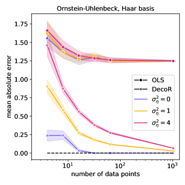
Figure 5: Synthetic experiment where $\epsilon_{x}$ and $U$ are generated by two independent Ornstein-Uhlenbeck processes and we choose $\phi$ to be the Haar basis.

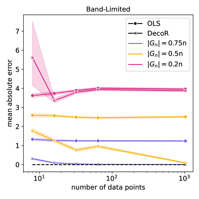
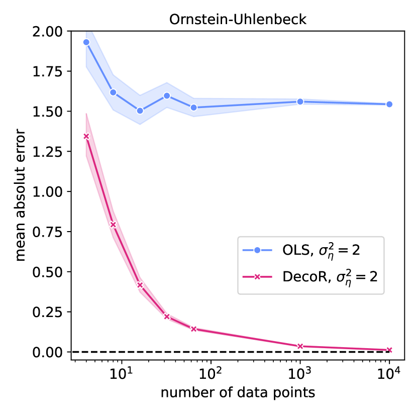
Figure 6: Left: Synthetic experiment where $\epsilon_{x}$ and $U$ are generated by two independent band-limited processes. Right: Synthetic experiment where $\epsilon_{x}$ and $U$ are generated by two independent Ornstein-Uhlenbeck processes. For this experiment we add i.i.d. standard Gaussian noise to $U$, which makes the confounder dense and, therefore, the model is misspecified (cf. Setting 1).

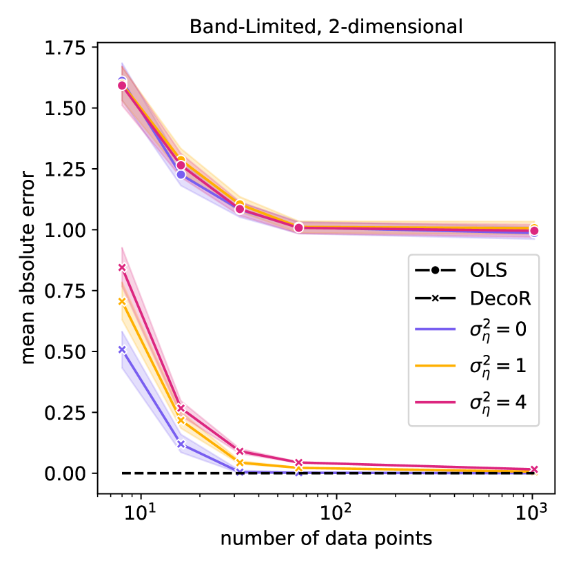
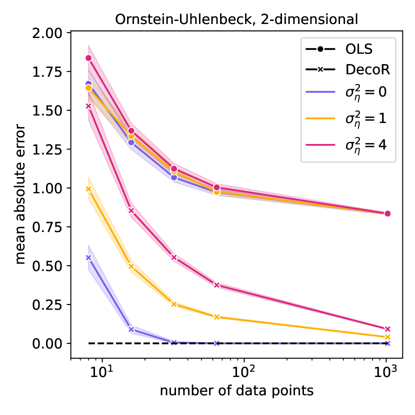
Figure 7: Left: Synthetic experiment where $\epsilon_{x}$ is generated by a 2-dimensional band-limited process and $U$ by a 1-dimensional band-limited process. Right: Synthetic experiment where $\epsilon_{x}$ is generated by a 2-dimensional Ornstein-Uhlenbeck process and $U$ by a 1-dimensional Ornstein-Uhlenbeck process.

$n$	mean	min	max
10	2.42	2	3
100	5.14	3	8
1000	8.26	4	13

Figure 8: Number of iterations until convergence for DecoR-Tor. Even for sample size $n=1000$, DecoR converges after $<15$ iterations.

References

- Ahmed et al. (1974) N. Ahmed, T. Natarajan, and K. R. Rao. Discrete cosine transform. IEEE transactions on Computers, 100(1):90–93, 1974.
- Angrist and Pischke (2009) J. D. Angrist and J.-S. Pischke. Mostly harmless econometrics: An empiricist’s companion. Princeton University Press, 2009.
- Bhatia et al. (2015) K. Bhatia, P. Jain, and P. Kar. Robust regression via hard thresholding. Advances in Neural Information Processing Systems, 28, 2015.
- Bhatia et al. (2017) K. Bhatia, P. Jain, P. Kamalaruban, and P. Kar. Consistent robust regression. Advances in Neural Information Processing Systems, 30, 2017.
- Bowden and Turkington (1990) R. Bowden and D. Turkington. Instrumental Variables. Econometric Society Monographs. Cambridge University Press, 1990.
- Ćevid et al. (2020) D. Ćevid, P. Bühlmann, and N. Meinshausen. Spectral deconfounding via perturbed sparse linear models. The Journal of Machine Learning Research, 21(1):9442–9482, 2020.
- Chen et al. (2013) Y. Chen, C. Caramanis, and S. Mannor. Robust sparse regression under adversarial corruption. In International Conference on Machine Learning, pages 774–782, 2013.
- Clayton et al. (1993) D. G. Clayton, L. Bernardinelli, and C. Montomoli. Spatial correlation in ecological analysis. International journal of epidemiology, 22(6):1193–1202, 1993.
- Diakonikolas et al. (2019) I. Diakonikolas, W. Kong, and A. Stewart. Efficient algorithms and lower bounds for robust linear regression. In Proceedings of the Thirtieth Annual ACM-SIAM Symposium on Discrete Algorithms, pages 2745–2754, 2019.
- Dupont et al. (2022) E. Dupont, S. N. Wood, and N. H. Augustin. Spatial+: a novel approach to spatial confounding. Biometrics, 78(4):1279–1290, 2022.
- d’Orsi et al. (2021) T. d’Orsi, G. Novikov, and D. Steurer. Consistent regression when oblivious outliers overwhelm. In International Conference on Machine Learning, pages 2297–2306, 2021.
- Fair (1970) R. C. Fair. The estimation of simultaneous equation models with lagged endogenous variables and first order serially correlated errors. Econometrica: Journal of the Econometric Society, pages 507–516, 1970.
- Guan et al. (2023) Y. Guan, G. L. Page, B. J. Reich, M. Ventrucci, and S. Yang. Spectral adjustment for spatial confounding. Biometrika, 110(3):699–719, 2023.
- Haar (1909) A. Haar. Zur theorie der orthogonalen funktionensysteme. Georg-August-Universitat, Gottingen., 1909.
- Huber (1964) P. J. Huber. Robust Estimation of a Location Parameter. The Annals of Mathematical Statistics, 35(1):73 – 101, 1964.
- Hughes and Haran (2013) J. Hughes and M. Haran. Dimension reduction and alleviation of confounding for spatial generalized linear mixed models. Journal of the Royal Statistical Society Series B: Statistical Methodology, 75(1):139–159, 2013.
- Janzing et al. (2009) D. Janzing, J. Peters, J. Mooij, and B. Schölkopf. Identifying confounders using additive noise models. In Proceedings of the Twenty-Fifth Conference on Uncertainty in Artificial Intelligence, page 249–257, 2009.
- Keller and Szpiro (2020) J. P. Keller and A. A. Szpiro. Selecting a scale for spatial confounding adjustment. Journal of the Royal Statistical Society Series A: Statistics in Society, 183(3):1121–1143, 2020.
- Klivans et al. (2018) A. Klivans, P. K. Kothari, and R. Meka. Efficient algorithms for outlier-robust regression. In Conference On Learning Theory, pages 1420–1430, 2018.
- Mahecha et al. (2010) M. D. Mahecha, M. Reichstein, N. Carvalhais, G. Lasslop, H. Lange, S. I. Seneviratne, R. Vargas, C. Ammann, M. A. Arain, A. Cescatti, et al. Global convergence in the temperature sensitivity of respiration at ecosystem level. Science, 329(5993):838–840, 2010.
- Marques et al. (2022) I. Marques, T. Kneib, and N. Klein. Mitigating spatial confounding by explicitly correlating gaussian random fields. Environmetrics, 33(5):2727, 2022.
- Newey and West (1987) W. K. Newey and K. D. West. A simple, positive semi-definite, heteroskedasticity and autocorrelation consistent covariance matrix. Econometrica, 55(3):703–708, 1987.
- Paciorek (2010) C. J. Paciorek. The importance of scale for spatial-confounding bias and precision of spatial regression estimators. Statistical Science: A Review Journal of the Institute of Mathematical Statistics, 25(1):107, 2010.
- Page et al. (2017) G. L. Page, Y. Liu, Z. He, and D. Sun. Estimation and prediction in the presence of spatial confounding for spatial linear models. Scandinavian Journal of Statistics, 44(3):780–797, 2017.
- Pearl (2009) J. Pearl. Causality. Cambridge University Press, 2009.
- Pensia et al. (2020) A. Pensia, V. Jog, and P.-L. Loh. Robust regression with covariate filtering: Heavy tails and adversarial contamination. arXiv preprint arXiv:2009.12976, 2020.
- Peters et al. (2017) J. Peters, D. Janzing, and B. Schölkopf. Elements of Causal inference: Foundations and Learning Algorithms. The MIT Press, 2017.
- Prates et al. (2019) M. O. Prates, R. M. Assunção, and E. C. Rodrigues. Alleviating spatial confounding for areal data problems by displacing the geographical centroids. Bayesian Analysis, 14(2):623 – 647, 2019.
- Reich et al. (2006) B. J. Reich, J. S. Hodges, and V. Zadnik. Effects of residual smoothing on the posterior of the fixed effects in disease-mapping models. Biometrics, 62(4):1197–1206, 2006.
- Reiersøl (1945) O. Reiersøl. Confluence Analysis by Means of Instrumental Sets of Variables. PhD thesis, Almqvist & Wiksell, 1945.
- Rubin (2005) D. B. Rubin. Causal inference using potential outcomes: Design, modeling, decisions. Journal of the American Statistical Association, 100(469):322–331, 2005.
- Sasai and Fujisawa (2020) T. Sasai and H. Fujisawa. Robust estimation with lasso when outputs are adversarially contaminated. arXiv preprint arXiv:2004.05990, 2020.
- Scheidegger et al. (2023) C. Scheidegger, Z. Guo, and P. Bühlmann. Spectral deconfounding for high-dimensional sparse additive models. arXiv preprint arXiv:2312.02860, 2023.
- Sippel et al. (2019) S. Sippel, N. Meinshausen, A. Merrifield, F. Lehner, A. G. Pendergrass, E. Fischer, and R. Knutti. Uncovering the forced climate response from a single ensemble member using statistical learning. Journal of Climate, 32(17):5677–5699, 2019.
- Suggala et al. (2019) A. S. Suggala, K. Bhatia, P. Ravikumar, and P. Jain. Adaptive hard thresholding for near-optimal consistent robust regression. In Conference on Learning Theory, pages 2892–2897, 2019.
- Thaden and Kneib (2018) H. Thaden and T. Kneib. Structural equation models for dealing with spatial confounding. The American Statistician, 72(3):239–252, 2018.
- Thams et al. (2022) N. Thams, R. Søndergaard, S. Weichwald, and J. Peters. Identifying causal effects using instrumental time series: Nuisance IV and correcting for the past. arXiv preprint arXiv:2203.06056, 2022.
- Vershynin (2018) R. Vershynin. High-Dimensional Probability: An Introduction with Applications in Data Science. Cambridge University Press, 2018.
- Wright (1928) P. Wright. The Tariff on Animal and Vegetable Oils. Macmillan, 1928.