On the Hölder Stability of
Multiset and Graph Neural Networks

Abstract

Famously, multiset neural networks based on sum-pooling can separate all distinct multisets, and as a result can be used by message passing neural networks (MPNNs) to separate all pairs of graphs that can be separated by the 1-WL graph isomorphism test. However, the quality of this separation may be very weak, to the extent that the embeddings of "separable" multisets and graphs might even be considered identical when using fixed finite precision.

In this work, we propose to fully analyze the separation quality of multiset models and MPNNs via a novel adaptation of Lipschitz and Hölder continuity to parametric functions. We prove that common sum-based models are lower-Hölder continuous, with a Hölder exponent that decays rapidly with the network’s depth. Our analysis leads to adversarial examples of graphs which can be separated by three 1-WL iterations, but cannot be separated in practice by standard maximally powerful MPNNs. To remedy this, we propose two novel MPNNs with improved separation quality, one of which is lower Lipschitz continuous. We show these MPNNs can easily classify our adversarial examples, and compare favorably with standard MPNNs on standard graph learning tasks.

1 Introduction

Motivated by a multitude of applications, including molecular systems [20], social networks [8], recommendation systems [19] and more, permutation invariant deep learning for both multisets and graphs have gained increasing interest in recent years. This in turn has inspired several theoretical works analyzing common permutation invariant models, and their expressive power and limitations.

For multiset data, it is known that simple summation-based multiset functions are injective, and as a result, can approximate all continuous functions on multisets [37]. These results have been discussed and strengthened in many different recent publications [33, 1, 30].

For graph neural networks (GNNs) the situation is more delicate, as all known graph neural networks with polynomial complexity have limited expressive power. Our focus in this paper will be on the Message Passing Neural Network (MPNN) [20] paradigm, which includes a variety of popular GNNs [35, 20, 25]. In their seminal works, [35, 28] prove that MPNNs are at most capable of separating graphs that can be separated by the Weisfeiler-Lehman (WL) graph isomorphism test [34]. Accordingly, maximally expressive MPNNs are those which are able to separate all graph pairs which are WL-separable. In [35, 28], it is shown that MPNNs which employ injective multiset functions are maximally expressive.

The theoretical ability of a permutation invariant network to separate a pair of objects (multisets/graphs) is a necessary condition for all learning tasks which require such separation, e.g., binary classification tasks where the two objects have opposite labels. However, while current theory ensures separation, it tells us little about the separation quality, so that embeddings of "separable" objects may be extremely similar, to the extent that in some cases, graphs which can be theoretically separated by maximally expressive MPNNs are completely identical on a computer with fixed finite precision (see [9], figure 1).

To study separation quality of permutation invariant models, we will search for bi-Hölder continuity guarantees. For metric spaces $(X,d_{X})$ and $(Y,d_{Y})$, a function $f:X\to Y$ is $\beta$ upper-Hölder continuous and $\alpha$ lower-Hölder continuous if there exists some positive constants $c,C$ such that

$$cd_{X}(x,x^{\prime})^{\alpha}\leq d_{Y}(f(x),f(x^{\prime}))\leq Cd_{X}(x,x^{\prime})^{\beta},\forall x,x^{\prime}\in X.$$

The upper and lower Hölder conditions guarantee that embedding distances in $Y$ will not be much larger, or much smaller, than distances in the original space $X$ (in our case a space of multisets or graphs). A function $f$ will have higher separation quality the closer the Hölder exponents are to one. When $\beta=1$ we say $f$ is (upper) Lipschitz, and when $\alpha=1$ we say that $f$ is lower Lipschitz.

We next describe our main results. We note that all models we consider are upper Lipschitz, so the remainder of this section will focus on lower Hölder exponents.

Main results: multisets

We begin with considering a rather standard approach [37]: multiset functions based on summation of point-wise applied neural networks, as in (1) below. Recent work has shown that when using smooth activations these functions are injective but not lower-Lipschitz, and when using ReLU activations they are not even injective, and therefore not lower-Hölder for any parameter choice of the network. This result motivates our novel definition of ’lower-Hölder in expectation’ for parametric functions, where the expectation is taken over the parameters.

With respect to our new relaxed notion of lower-Hölder continuity, we show that ReLU summation multiset networks have an expected lower-Hölder exponent of $\alpha=3/2$. Surprisingly, while smooth activations lead to injectivity [1], we find that their expected Hölder exponent is much worse: at best it is equal to the maximal number of elements in the multiset data, $\alpha\geq n$.

The relatively moderate exponent $\alpha=3/2$ of ReLU networks is guaranteed only when the range of the bias of the network contains the range of the multiset features, an assumption which may be problematic to fulfill in practice. To address this, we suggest an Adaptive ReLU summation network, where the bias is adapted to the values in the multiset. This network is guaranteed the same $3/2$ exponent while overcoming the range issue.

Finally, we consider multiset functions based on linear functions and column-wise sorting. Building on known results from [2], we show that such networks are lower Lipschitz in expectation.

Model	bounds
relu sum	$\alpha=3/2$
adaptive relu	$\alpha=3/2$
smooth sum	$n\leq\alpha$
sort based	$\alpha=1$
ReluMPNN	$\frac{3}{2}+\frac{K+1}{2}\leq\alpha\leq(\frac{3}{2})^{K+1}$
AdaptMPNN	$\alpha\leq(\frac{3}{2})^{K+1}$
SortMPNN	$\alpha=1$
SmoothMPNN	$2^{K+1}\leq\alpha$
SortMPNN	$\alpha=1$

Table 1: Summary of lower-Hölder exponent bounds for multiset (top) and graph (bottom) models.

Main Results: MPNNs

Next, we consider expected Hölder continuity of MPNNs for graphs. We note that while the Lipschitz property of MPNNs like GIN [35] was established in [14], lower Lipschitz or Hölder guarantees have not been addressed to date. Indeed, a recent survey [26] lists bi-Lipschitz guarantees for MPNNs as one of the future challenges for theoretical GNN research.

We derive bounds on the expected lower-Hölder exponent of MPNNs based on sum pooling that show the exponent grows with the depth $K$, potentially exponentially. In contrast, we suggest a new MPNN architecture we name SortMPNN, which uses a continuous sort based aggregation, resulting in SortMPNN being lower-Lipschitz in expectation. The exponent bounds of both the graph and multiset models appear in table 1.

Our analysis provides an adversarial example where the expected lower-Hölder exponent of sum-based MPNNs indeed grows exponentially worse with depth. We show in Table 2 that sum-based MPNNs fail to learn a simple binary classification task on such data, while SortMPNN and AdaptMPNN, which is based on adaptive ReLU, handle this task easily. We also provide experiments on several graph datasets which show that SortMPNN often outpreforms standard MPNNs on non-adversarial data.

1.0.1   Notation

$S^{d-1}$ denotes the unit sphere $\{x\in\mathbb{R}^{d}|\quad\|x\|_{2}=1\}$. The notation ’$a\sim S^{d-1}$ and $b\sim[-B,B]$’ implies that the distribution on $a$ (respectively $b$) is taken to be uniform on $S^{d-1}$ (respectively $[-B,B]$), and that $a$ and $b$ are drawn independently. The inner product of two vectors $a,b$ is denoted by $a\cdot b$.

2 General framework

In this section, we present the framework for analyzing separation quality of parametric functions. We begin by extending the notion of Hölder continuity to a family of parametric functions.

2.1 upper-Hölder and lower continuity in expectation

Let $(X,d_{X})$ and $(Y,d_{Y})$ be metric spaces, let $W$ be some set of parameters, and let $f(x;w):X\times W\to Y$ be a parametric function. we say that $f(x;w)$ is uniformly Lipschitz with constant $L>0$, if for all $w\in W$, the function $x\mapsto f(x;w)$ is $L$-Lipschitz. This definition can naturally be extended to other upper-Hölder exponents, but this will not be necessary as the parametric functions we discuss in this paper will all end up being uniformly Lipschitz.

As mentioned in the introduction, the situation for lower continuity is different, as for sum-based ReLU networks no fixed choice of parameters will yield a truly lower-Hölder function. Nonetheless, these networks do perform well both in learning tasks and in empirical metric distortion tests ([1], Figure 2), suggesting that the standard notion of lower-Hölder continuity may be too stringent. To address this concern, we introduce the notion of lower-Hölder continuity in expectation:

Definition 2.1.

Let $\alpha>0,p\geq 1$. Let Let $(X,d_{X})$ and $(Y,d_{Y})$ be metric spaces, and let $(W,\mathcal{B},\mu)$ be a probability space. Let $f(x;w):X\times W\to Y$ be a parametric function, so that for every fixed $x\in X$ the function $f(x;\cdot)$ is measurable. We say that $f$ is $\alpha$ lower-Hölder continuous in expectation if there exists a strictly positive $c$ such that

$$c^{p}\leq\mathbb{E}_{w\sim\mu}\left\{\frac{d_{Y}(f(x;w),f(x^{\prime};w))}{d_{X}(x,x^{\prime})^{\alpha}}\right\}^{p},\quad\forall(x,x^{\prime})\in X\times X,\text{ with }d(x,x^{\prime})>0$$

A few remarks on this definition are in order. Firstly, we note this generalizes the standard definition since a family of lower-Hölder functions $f(x;w)$ ($\alpha$ lower-Hölder for any choice of $w$), will lead to $f(x;w)$ being $\alpha$ lower-Hölder in expectation. Next, we note that our definition takes an expectation over the parameters, but requires uniform boundedness over $x,x^{\prime}$ pairs. This choice was made since the parameter distribution can be chosen by the algorithm, at least at initialization, while the data distribution is unknown. To further validate this decision, we show later in table 2 that even with training, models with a high lower-Hölder exponent in expectation, fail to learn hard tasks. Thirdly, we note that as with the standard Hölder definitions, Hölder in expectation exponents that are closer to one will be regarded as having higher separation quality. Lastly, the results stated in the introduction are for the default $p=2$.

While the expected value across random parameters is informative as is, the variance can potentially have a strong effect on the separation in practice. Luckily, our analysis will typically apply for models $f(x;w)$ of width $1$, and models with width $W$ can be viewed as stacking of $W$ multiple model instances. Wider models will have the same expected distortion as the width one model, but the variance will converge to zero, in a rate proportional to $1/W$, as long as $d_{X}=l_{p}$ with the same $p$ used in definition 2.1. For more details on this effect see appendix B.1.

We now proceed to analyze the expected upper and lower Hölder continuity for parametric models on multisets, followed by an analysis on MPNNs.

3 Multiset Hölder Continuity

Standing assumptions: Throughout the rest of this section, we will say that $(n,d,p,\Omega,z)$ satisfy our standing assumptions, if $n,d$ are natural numbers, $p\geq 1$, the set $\Omega$ is a compact subset of $\mathbb{R}^{d}$, and $z$ will be a point in $\mathbb{R}^{d}\setminus\Omega$.

A multiset $\{\!\!\{x_{1},\ldots,x_{k}\}\!\!\}$ is a collection of $n$ unordered elements where (unlike sets) repetitions are allowed. We denote by $\mathcal{S}_{\leq n}(\Omega)$ and $\mathcal{S}_{=n}(\Omega)$ the space of all multisets with at most $n$ elements (respectively, exactly $n$ elements), which reside in $\Omega$.

A popular choice of a metric on $\mathcal{S}_{=n}(\Omega)$ is the Wasserstein metric

$${W}_{1}(\{\!\!\{x_{1},\ldots,x_{n}\}\!\!\},\{\!\!\{y_{1},\ldots,y_{n}\}\!\!\})=\min_{\tau\in S_{n}}\sum_{j=1}^{n}\|x_{j}-y_{\tau(j)}\|_{p}$$

Following [14], we extend the Wasserstein metric to the space $\mathcal{S}_{\leq n}(\Omega)$ by applying the augmentation map which adds the vector $z$ to a given multiset until it is of maximal size $n$:

$$\rho_{(z)}\left(\{\!\!\{x_{1},\ldots,x_{k}\}\!\!\}\right)=\{\!\!\{x_{1},\ldots,x_{k},x_{k+1}=z,\ldots.x_{n}=z\}\!\!\}$$

This induces the augmented Wasserstein metric $W_{1}^{z}$ on $\mathcal{S}_{\leq n}(\Omega)$,

$$W_{1}^{z}(S_{1},S_{2})=W_{1}(\rho_{(z)}(S_{1}),\rho_{(z)}(S_{2})),\quad S_{1},S_{2}\in\mathcal{S}_{\leq n}(\Omega)$$

Now that we have introduced the augmented Wasserstein as the metric we will use for multisets, we turn to analyze the multiset neural networks we are interested in.

A popular building block in architectures for multisets [37] ,as well as MPNNs [35, 29, 20], is based on summation of element-wise neural network application. For a given activation $\sigma:\mathbb{R}\to\mathbb{R}$, we define a parametric function $m_{\sigma}$ on multisets in $\mathcal{S}_{\leq n}(\Omega)$, with parameters $(a,b)\in\mathbb{R}^{d}\oplus\mathbb{R}$, by

$$m_{\sigma}(\{\!\!\{x_{1},\ldots,x_{r}\}\!\!\};a,b)=\sum_{i=1}^{r}\sigma(a\cdot x_{i}-b).$$ (1)

We note that we focus on $m_{\sigma}$ with scalar outputs, since the variant with vector output has the same Hölder properties, as discussed in the end of Section 2.

3.0.1   ReLU summation

We set out to understand the expected Hölder continuity of $m_{\sigma}$, starting from the case $\sigma=\mathrm{ReLU}$:

theoremReluMoments For $(n,d,p,\Omega,z)$ satisfying our standing assumptions, assume that $a\sim S^{d-1}$ and $b\sim[-B,B]$. Then $m_{ReLU}$ is uniformly Lipschitz. Moreover,

1. $m_{ReLU}$ is not $\alpha$ lower-Hölder continuous in expectation for any $\alpha<\frac{p+1}{p}$.

2. If $\|x\|<B$ for all $x\in\Omega$, then $m_{ReLU}$ is $\frac{p+1}{p}$ lower-Hölder continuous in expectation.

Proof idea: the $\pm\epsilon$ example.

The following example, which we nickname the $\pm\epsilon$ example, gives a good intuition for the Hölder behavior of $m_{\mathrm{ReLU}}$. Denote $X_{\epsilon}=\{\!\!\{-\epsilon,\epsilon\}\!\!\}$ and $X_{2\epsilon}=\{\!\!\{-2\epsilon,2\epsilon\}\!\!\}$. The Wasserstein distance between these two multisets is proportional to $\epsilon$. Now, let us consider the images of these multisets under $m_{\mathrm{ReLU}}$, where we assume for simplicity that $d=1$ and $a=1$. Note that when $b>2\epsilon$ we will get $ReLU(x-b)=0$ for all $x$ in either sets, and so $m_{\mathrm{ReLU}}(X_{2\epsilon};1,b)=m_{\mathrm{ReLU}}(X_{\epsilon};1,b)$. We will get a similar results when $b\leq-2\epsilon$. In this case, for every $x\geq-2\epsilon$ we have $\mathrm{ReLU}(x-b)=x-b$. Therefore, we will obtain that

$$m_{\mathrm{ReLU}}(X_{2\epsilon};1,b)=(-2\epsilon-b)+(2\epsilon-b)=(-\epsilon-b)+(\epsilon-b)=m_{\mathrm{ReLU}}(X_{\epsilon};1,b),\quad\forall b<-2\epsilon.$$

We conclude that $|m_{\mathrm{ReLU}}(X_{2\epsilon};1,b)-m_{\mathrm{ReLU}}(X_{\epsilon};1,b)|^{p}$ is zero for all $b$ outside the interval $(-2\epsilon,2\epsilon)$. Inside this interval of length $4\epsilon$, we will typically have $|m_{\mathrm{ReLU}}(X_{2\epsilon};1,b)-m_{\mathrm{ReLU}}(X_{\epsilon};1,b)|^{p}\sim\epsilon^{p}$, so that the expectation over all $b$ will be proportional to $4\epsilon\cdot\epsilon^{p}\sim\epsilon^{p+1}$. To ensure that the ratio between $\epsilon^{p+1}$ and $W_{p}(X_{2\epsilon},X_{\epsilon})^{\alpha p}\sim\epsilon^{\alpha p}$ will have a strictly positive lower bound as $\epsilon\rightarrow 0$ , we need to choose $\alpha\geq\frac{p+1}{p}$. The proof that $\alpha=\frac{p+1}{p}$ is actually enough, and several other details necessary to turning this argument into a full proof, are given in the appendix.

3.0.2   Adaptive ReLU

To attain the $(p+1)/p$ exponent in theorem 3.0.1, we need to assume that the bias is drawn from an interval $[-B,B]$ which is large enough so that all features $a\cdot x$ will necessarily reside in it. This assumption may be difficult to satisfy, especially in MPNNs where the features in intermediate layers are effected by previous parameter choices. Additionally, the $\pm\epsilon$ example shows that when $b$ is outside the range of the multiset features, $m_{\mathrm{ReLU}}$ is not effective. Motivated by these observations, we propose a novel parametric function for multisets, based on $\mathrm{ReLU}$, where the bias is automatically adapted to feature values. For a multiset $X=\{\!\!\{x_{1},\ldots,x_{r}\}\!\!\}$ and $a\in\mathbb{R}^{d},t\in[0,1]$, the adaptive $\mathrm{ReLU}$ function $m_{\mathrm{ReLU}}^{\mathrm{adapt}}(X;a,t)$ is defined using $m=\min\{a\cdot x_{1},\ldots,a\cdot x_{r}\},M=\max\{a\cdot x_{1},\ldots,a\cdot x_{r}\},b=(1-t)m+tM$ and

$$m_{\mathrm{ReLU}}^{\mathrm{adapt}}(X;a,t)=[r,m,M,\frac{1}{r}\sum_{i=1}^{r}\mathrm{ReLU}(a\cdot x_{i}-b)]$$

The output of $m_{\mathrm{ReLU}}^{\mathrm{adapt}}$ is a four dimensional vector . The last coordinate of the vector is essentially $m_{\mathrm{ReLU}}$, where the bias $b$ now only varies between the minimal and maximal value of multiset features. The first three coordinates are simple invariant features of the multisets: its cardinality and minimal and maximal value. In the appendix we prove theoremAdaptiveRelu For $(n,d,p,\Omega,z)$ satisfying our standing assumptions, assume that $a\sim S^{d-1}$ and $t\sim[0,1]$. Then the function $m_{\mathrm{ReLU}}^{\mathrm{adapt}}:\mathcal{S}_{\leq n}(\Omega)\times S^{d-1}\times[0,1]\to\mathbb{R}^{4}$ is uniformly Lipschitz and $\frac{p+1}{p}$ lower-Hölder continuous in expectation.

We note that while adaptive ReLU solves the $\pm\epsilon$ example, a similar issue can be created for adaptive ReLU with multisets such as $\{\!\!\{1,0,0,-1\}\!\!\}$ and $\{\!\!\{1,\epsilon,-\epsilon,-1\}\!\!\}$, which force the adaptive bias to cover the interval $[1,1]$. Nonetheless, the delicate bias range assumption is no longer an issue.

3.0.3   Summation with smooth activation

We now consider the Hölder properties of $m_{\sigma}$ when the activation $\sigma$ is smooth (e.g., sigmoid, SiLU, tanh). To understand this scenario, it can be instructive to first return to the $\pm\epsilon$ example. In this example, since the elements in $X_{\epsilon}$ and $X_{2\epsilon}$ both sum to the same number, one can deduce that (for any choice of bias) the first order Taylor expansion of $m_{\sigma}(X_{2\epsilon})-m_{\sigma}(X_{\epsilon})$ will vanish, so that this difference will be of the order of $\epsilon^{2}$. Based on this example we can already see that for smooth activations $\alpha\geq 2$. However, it turns out that there are adversarial examples with much worse behavior. Specifically, note that $X_{\epsilon}$ and $X_{2\epsilon}$ are ’problematic’ because their first moments are identical. In the same spirit, by choosing a pair $X,X^{\prime}$ of distinct multisets with $n$ elements in $\mathbb{R}$, whose first $n-1$ moments are identical, we can deduce that $\alpha\geq n$:

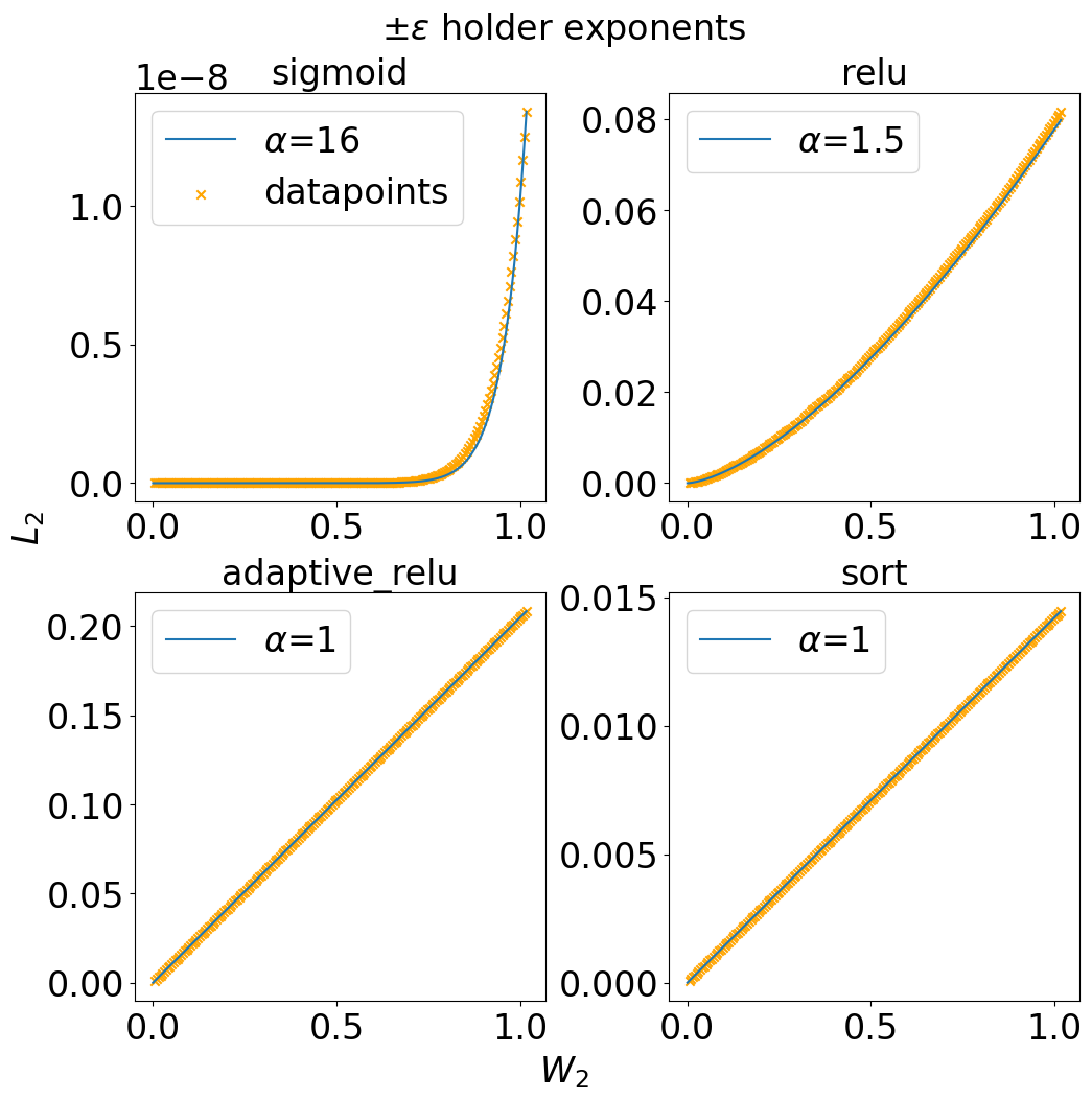
Figure 1: $l_{2}$ vs. $W_{2}$ distance on multiple adversarial multiset-pair with 15 identical moments. Results are in accordance with our theoretical results (see Table1)

theoremSmoothMoments Assume $(n,d,p,\Omega,z)$ satisfy our standing assumptions, $\sigma:\mathbb{R}\mapsto\mathbb{R}$ has $n$ continuous derivatives, and $a\sim S^{d-1},b\sim[-B,B]$. If the function $m_{\sigma}$ is $\alpha$ lower-Hölder continuous in expectation, then $\alpha\geq n$.

3.0.4   Sort based

We now present the fourth and final multiset parametric function which we would like to address. Based on ideas from [2, 18], we consider the parametric function

$$S_{z}(X;a,b)=\langle\mathrm{sort}(a\cdot\rho_{(z)}(X)),b\rangle$$ (2)

where $X\in\mathbb{R}^{d\times n}$ and $a,b$ are in $S^{d-1}$ and $S^{n-1}$ respectively. Note $S_{z}$ explicitly includes the augmentation by $z$, while in our previous discussions this was not necessary for expected Hölder continuity with respect to $W_{p}^{z}$. On the bright side, the sort-based parametric functions are lower-Lipschitz in expectation.

theoremSortHolder For $(n,d,p,\Omega,z)$ satisfying our standing assumptions. Assume that $a\sim S^{d-1}$ and $b\sim S^{n-1}$. Then $S(\cdot;a,b)$ is uniformly upper Lipschitz and lower Lipschitz in expectation.

The proof of this claim is that such mappings were shown to be bi-Lipschitz for all parameters, when duplicated enough times (with independent parameters) [2]. This implies bi-Lipschitzness in expectation for the duplicated function, which in turn implies bi-Lipschitzness in expectation for a single function since the relevant expectations are identical.

Summary

In Figure 1, we choose a pair of distinct multisets $X,X^{\prime}$ with $16$ scalar features each, which have $15$ identical moments (for details on how this was constructed see Subsection C.2 in the appendix). The figure plots the distance between embedding distances versus the Wasserstein distance, for pairs $\epsilon X,\epsilon X^{\prime}$, for varying values of $\epsilon$. The figure illustrates that the $\alpha=3/2$ Hölder exponent of ReLU (we take $p=2$) and the $\alpha\geq n$ exponent of sigmoid summation are indeed encountered in this example. The sort and adaptive ReLU methods display a linear plot in this case (recall that while sort is indeed lower-Lipschitz in expectation, adaptive ReLU is not, but showing for adaptive ReLU will require different adversarial examples).

4 MPNN Hölder Continuity

We will now analyze the expected Hölder continuity of MPNNs for graphs, using the various multiset embeddings discussed previously. We begin by defining MPNNs, WL tests, and the graph WL-metric of our choice.

4.1 MPNNs and WL

We denote a graph by $G=(V,E,X)$ where $V$ are the nodes, $E$ are the edges, and $X=(x_{v})_{v\in V}$ are the initial node features. Throughout this section we will assume, as in the previous section, that $\Omega$ is a compact subset of $\mathbb{R}^{d}$, and $z$ is some fixed point in $\mathbb{R}^{d}\setminus\Omega$. We denote the neighborhood of a node $v$ by $\mathcal{N}_{v}=\{\!\!\{u\in V|(u,v)\in E\}\!\!\}$. MPNNs iteratively use the graph structure to redefine node features in the following manner: initialize $x_{v}^{(0)}=x_{v}$.

For $\mathbf{k=1\ldots,K}$

$$\text{{AGGREGATE}: }c_{v}^{(k)}=\phi^{(k)}(\{\!\!\{x_{u}^{(k-1)}|u\in\mathcal{N}_{v}\}\!\!\})$$

$$\text{{COMBINE}: }x_{v}^{(k)}=\psi^{(k)}(x_{v}^{(k-1)},c_{v}^{(k)})$$

In order to achieve a final graph embedding, a final READOUT step is performed

$$\textit{READOUT}:c^{\mathrm{global}}=\eta(\{\!\!\{x_{v}^{(K)}|v\in V\}\!\!\})$$

We note that different instantiations of the COMBINE, AGGREGATE, and READOUT parametric functions will lead to different architectures. We will discuss several choices, and their expected Hölder continuity properties, slightly later on. Once such an instantiation is chosen, an MPNN will be a parametric model of the form $f(G;w)=c^{\mathrm{global}}$, where $w$ denotes the concatenation of all parameters of the COMBINE, AGGREGATE, and READOUT functions.

The Weisfeiler-Lehman (WL) graph isomorphism test [34, 24] checks whether two graphs $G,G^{\prime}$ are isomorphic (identical up to node permutation) by applying an MPNN-like procedure while choosing the COMBINE, AGGREGATE and READOUT functions to be hash functions, and running the procedure for at most $K=max\{|V_{G}|,|V_{H}|\}$ [28] iterations, where $G,H$ are the graphs being tested for isomorphism. The WL test can separate many, but not all, pairs of non-isomorphic graphs.

Notably, MPNNs can only separate pairs of graphs which are WL separable, and therefore if we hope for MPNN Hölder continuity, we need to choose a WL metric: a pseudo-metric on graphs which is zero if and only if the pair of graphs cannot be separated by WL. Of the several possible choices in the recent literature for such a metric [21, 6, 13], we choose the Tree Mover’s Distance (TMD) suggested in [14]. This metric is based on a tree distance between the WL computation trees, which can be written recursively as the sum of the distance between tree roots $r$ and the augmented Wasserstein between the subtrees rooting at $r$’s children. For a detailed description of the TMD see Appendix E.

4.2 MPNN analysis

It would seem natural to expect that if the AGGREGATE, COMBINE and READOUT functions used in the MPNN are Hölder in expectation, then the overall MPNN will be Hölder in expectation as well. The following theorem will prove that this is indeed the case. In this theorem we will assume that the graph has at most $n$ nodes, and its features reside in a compact set $\Omega\subseteq\mathbb{R}^{d}$. We denote the space of all such graphs by $G_{\leq n}(\Omega)$.

theoremHolderMPNN (Hölder MPNN embeddings, informal version) Let $p\geq 1$, given an MPNN $f:G_{\leq n}(\Omega)\rightarrow\mathbb{R}^{m}$ with $K$ message passing layers followed by a $READOUT$ layer,

1. If the functions used for the aggregation $\phi^{(k)}$, combine $\psi^{(k)}$, and readout $\eta$ are $\alpha_{k},\beta_{k}$ and $\gamma$ lower Hölder continuous in expectation, then $f$ is lower Hölder continuous in expectation with an exponent $\gamma\cdot\prod_{k=1}^{K}(\alpha_{k}\cdot\beta_{k})$.

2. If all the above functions are uniformly upper Lipschitz, then $f$ is uniformly upper Lipschitz.

We note that the formal version of the theorem which we state and prove in the appendix includes a similar claim regarding node embeddings.

Defining an MPNN which uses Hölder ’building blocks’ is rather straightforward. The COMBINE function is a vector-to-vector function which can easily be chosen to be uniformly Lipschitz, and lower Lipschitz in expectation. One possible choice is just a linear function $x_{v}^{(k)}=Ax_{v}^{(k-1)}+Ba_{v}^{(k)}.$ In the appendix we prove the Lipschitz properties of this and three other combine choices.

The AGGREGATE and READOUT functions are multiset to vector functions, and we have discussed the Hölder properties of four different such choices in Section 3. In practice, at each iteration $k$ we take $W_{k}$ parallel copies of these functions with independent parameters ($W$ corresponds to the width of the MPNN). As discussed in the end of Subsection 2.1, this maintains the same results in expectation while reducing the variance. For example, the SortMPNN architecture will be defined using the sort-based parametric functions $S_{z}$ from (2) as

SortMPNN: For $\mathbf{k=1\ldots,K}$

$$\text{{AGGREGATE}: }c_{v,i}^{(k)}=S_{z_{k}}\left(\{\!\!\{x_{u}^{(k-1)}|u\in\mathcal{N}_{v}\}\!\!\};a_{i}^{(k)},b_{i}^{(k)}\right),\quad i=1,\ldots W_{k}$$

$$\text{{COMBINE}: }x_{v}^{(k)}=A^{(k)}x_{v}^{(k-1)}+B^{(k)}a_{v}^{(k)}$$

and the READOUT function is given by

$$\textit{READOUT}:c^{\mathrm{global}}_{i}=S_{z_{K+1}}\left(\{\!\!\{x_{v}^{(K)}|v\in V\}\!\!\};a_{i}^{(K+1)},b_{i}^{(K+1)}\right),\quad i=1,\ldots,W_{K+1}$$

Similarly, we will use the terms AdaptMPNN, ReluMPNN and SmoothMPNN to denote the MPNN obtained by replacing $S_{z}$ with the appropriate functions $m_{\mathrm{ReLU}}^{\mathrm{adapt}}$, $m_{\mathrm{ReLU}}$ or $m_{\sigma}$ with a smooth $\sigma$. corollarycormpnn(informal) Let $p\geq 1$,

1. SortMPNN is uniformly upper Lipschitz, and lower Lipschitz in expectation.

2. AdaptMPNN and ReluMPNN are uniformly upper Lipschitz, and $[(p-1)/p]^{K+1}$ lower-Hölder in expectation (where $K$ denotes the depth of the MPNN).

A full formal statement of this theorem is given in appendix G. The main missing detail is specifying the distribution on the parameters necessary to make this theorem work.

We note that the corollary supplies us with an upper bound on the optimal $\alpha_{*}$ for ReluMPNN and AdaptMPNN. We provide lower bounds for the Hölder exponents of ReluMPNN and SmoothMPNN using an adversarial set of examples we call $\epsilon$-Trees. These are defined recursively, where the first set of trees are of height two, and the leaves contain the $\pm\epsilon$ multisets. Deeper trees are then constructed by building upon substructures from the trees in the previous step as depicted in figure 6 alongside a rigorous formulation and proof in appendix H. This adversarial example allows us to prove for both ReluMPNN and SmoothMPNN that the Hölder exponent increases with depth.

theoremlb Assume that ReluMPNN with depth $K$ is $\alpha$ lower-Hölder in expectation, then $\alpha\geq 1+\frac{K+1}{p}$. If SmoothMPNN with depth $K$ is $\alpha$ lower-Hölder in expectation then $\alpha\geq 2^{K+1}$.

5 Experiments

In the following experiments, we evaluate the four architectures SortMPNN, AdaptMPNN, ReluMPNN and SmoothMPNN. As the last two architectures closely resemble standard MPNN like GIN [35] with ReLU/smooth activation, our focus is mainly on the SortMPNN and AdaptMPNN architectures. In our experiments we consider several variations of these architectures which were omitted in the main text for brevity, and are described in appendix I alongside further experiment details.

$\epsilon$-Tree dataset

Model	Accuracy
GIN[35]	0.5
GCN[25]	0.5
GAT[32]	0.5
ReluMPNN	0.5
SmoothMPNN	0.5
SortMPNN	1.0
AdaptMPNN	1.0

Table 2: $\epsilon$-Tree binary classification results

In order to show that the expected (lower) Hölder exponent is indeed a good indicator of separation quality, and to further validate the importance of separation quality analysis, we first focus on the adversarial $\epsilon$-tree construction used to prove Theorem 4.2.

To begin with, we show how randomly initialized MPNNs with the different multiset embeddings we analyzed distort the TMD metric on the $\epsilon$-trees. In figure 2 we see how the lower-Hölder exponent increases exponentially with depth for MPNNs using embeddings that are targeted by this adversarial dataset. Note that the behavior of ReluMPNN and SmoothMPNN is consistent with the $\alpha=(3/2)^{K+1}$ and $2^{K+1}$ bounds suggested by our theory for $p=2$.

We then proceed to train a binary classifier using these MPNNs in an attempt to separate the tree pairs.

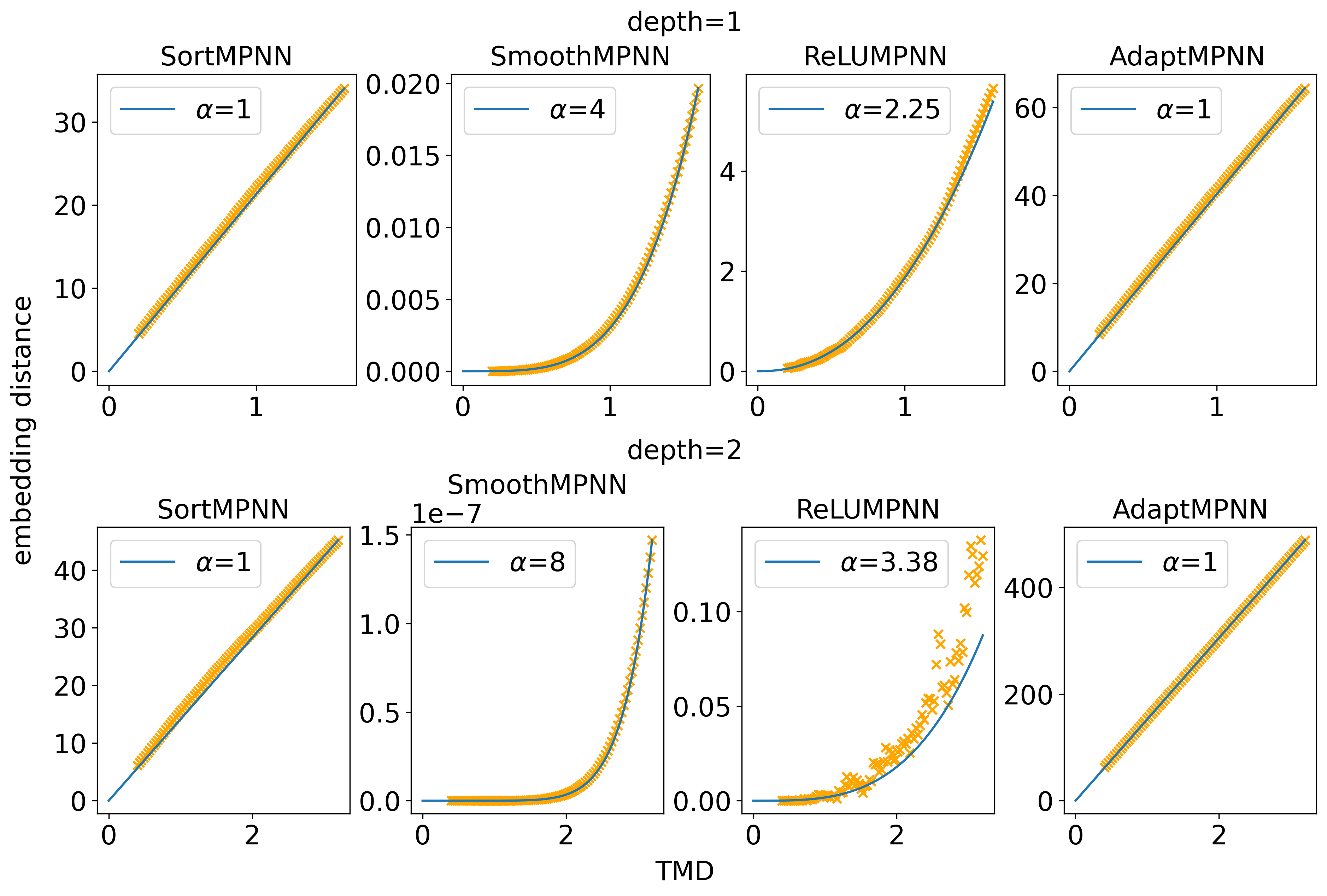
Figure 2: $l_{2}$ vs. TMD on $\epsilon$-Trees. The targeted ReluMPNN and SmoothMPNN exponents deteriorate with depth, in accordance with our theory (see Table 1)

The results in Table 2 show how only MPNNs with Lipschitz distortion on the dataset are able to achieve separation, while those with high exponents, in addition to several baseline MPNNs completely fail. This serves as proof to the importance of separation quality analysis, especially in light of the fact smooth activation MLP moments [1] and GIN [35] are in theory capable of separation.

TUDataset

While the $\epsilon$-Tree dataset emphasizes the importance of high separation quality, validating our analysis, it is not obvious what effect this has in real world datasets, where we don’t necessarily know how the exponent behaves. Therefore, we test SortMPNN and AdaptMPNN on a subset of the TUDatasets [27], including Mutag, Proteins, PTC, NCI1 and NCI109. Table 3 shows that SortMPNN outperforms several baseline MPNNs (results are reported using the evaluation method from [35]). Note that in all experiments we only compare to Vanilla MPNNs, and not more expressive architectures which often do reach better results, at a higher computational cost.

Dataset	Mutag	Proteins	PTC	NCI1	NCI109
GIN[35]	89.4$\pm$5.6	76.2$\pm$2.8	64.6$\pm$7	82.7$\pm$1.7	82.2$\pm$1.6
GCN[25]	85.6$\pm$5.8	76$\pm$3.2	64.2$\pm$4.3	80.2$\pm$2.0	NA
GraphSage[22]	85.1$\pm$7.6	75.9$\pm$3.2	63.9$\pm$7.7	77.7$\pm$1.5	NA
SortMPNN	91.49$\pm$5.8	76.46$\pm$4.36	67.79$\pm$8.84	84.31$\pm$1	82.77$\pm$0.9
AdaptMPNN	90.99$\pm$5.3	75.83$\pm$4	64.56$\pm$7.32	83.41$\pm$0.9	81.12$\pm$2

Table 3: Classification accuracy on a variety of TUdatasets [27].

LRGB

We further evaluate our architectures on two larger datasets from LRGB [17]. The first, peptides-func, is a multi-label graph classification dataset. The second, peptides-struct consists of the same graphs as peptides-func, but with regression task. Results in table 4 show that SortMPNN and AdaptMPNN are favorable on peptides-func while falling behind on peptides-struct. Both experiments adhere to the 500K parameter constraint as in [17].

In addition, we reran the peptides-struct experiment with a 100K, 50K, 25K and 7K parameter budget. The results in figure 4 show SortMPNN and AdaptMPNN outperforming GCN for smaller models, with SortMPNN achieving top results.

Dataset	peptides-func (AP$\uparrow$)	peptides-struct (MAE$\downarrow$)
GINE[23]	0.6621$\pm$0.0067	0.2473$\pm$0.0017
GCN[25]	0.6860$\pm$0.0050	0.2460$\pm$0.0007
GatedGCN[10]	0.6765$\pm$0.0047	0.2477$\pm$0.0009
SortMPNN	0.6914$\pm$0.0056	0.2494$\pm$0.0021
AdaptMPNN	0.6876$\pm$0.0049	0.2499$\pm$0.0032

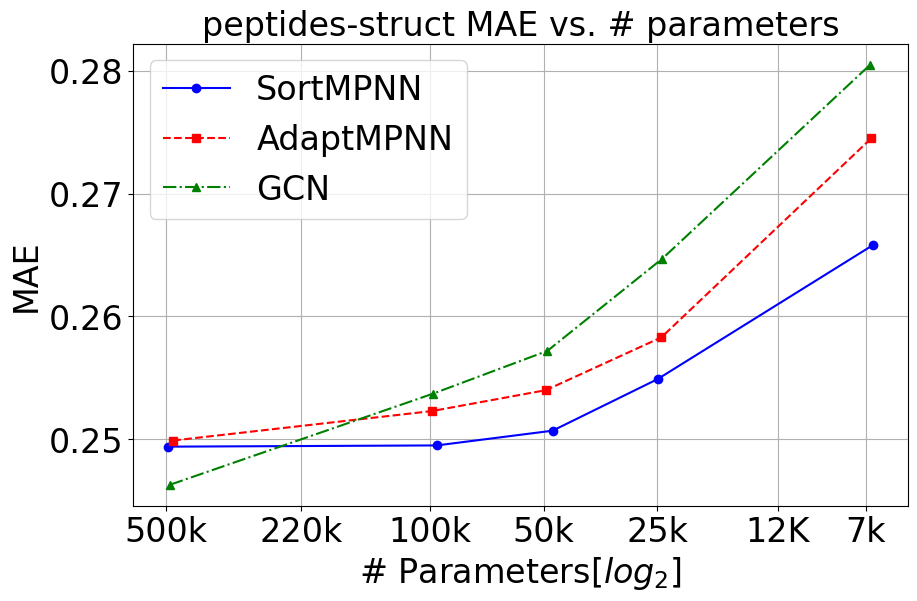
Figure 3: LRGB results. Best in bold.

Figure 4: pep-struct, #params vs. MAE

Subgraph aggregation networks - Zinc12K

To further evaluate the effect of our analysis, we experiment the use of our methods as part of the more advanced equivariant subgraph aggregation network (ESAN) [4], which has greater separation power than MPNNs.

To this extent, we run the experiment from [4] on the ZINC12K dataset, where we swap the base encoder from GIN [35] to SortMPNN and AdaptMPNN. The results shown in table 4 show that SortMPNN outperforms the other methods.

Method	GIN [35]	SortMPNN	AdaptMPNN
DS-GNN (ED)	0.172$\pm$0.008	0.160$\pm$0.019	0.178$\pm$0.009
DS-GNN (ND)	0.171$\pm$0.010	0.163$\pm$0.024	0.175$\pm$0.007
DS-GNN (EGO)	0.126$\pm$0.006	0.102$\pm$0.003	0.145$\pm$0.049
DS-GNN (EGO+)	0.116$\pm$0.009	0.111$\pm$0.006	0.129$\pm$0.007
DSS-GNN (ED)	0.172$\pm$0.005	0.159$\pm$0.007	0.170$\pm$0.005
DSS-GNN (ND)	0.166$\pm$0.004	0.145$\pm$0.008	0.164$\pm$0.010
DSS-GNN (EGO)	0.107$\pm$0.005	0.107$\pm$0.005	0.124$\pm$0.005
DSS-GNN (EGO+)	0.102$\pm$0.003	0.110$\pm$0.004	0.124$\pm$0.006

Table 4: ESAN [4] MAE per base encoder on ZINC12K. Best in bold.

For fair comparison, the models don’t surpass the 100K parameter budget.

6 Related work

Sorting

Sorting based operations were used for permutation invariant networks on multisets in [39], and as readout functions for MPNNs in [2, 38]. To the best of our knowledge, our SortMPNN is the first network using sorting for aggregations, and the first MPNN with provable bi-Lipschitz (in expectation) guarantees.

Bi-Lipschitz stability

An alternative bi-Lipschitz embedding for multisets was suggested in [12]. This embedding has higher computational complexity then sort based embedding. Some additional examples of recent works on bi-Lipschitz embeddings include [3, 12, 11].

We note that [7] does provide lower and upper continuity estimates for MPNNs with respect to a WL metric. These continuity estimates are in an $\epsilon-\delta$ sense, which do not rule out arbitrarily bad Hölder exponents. Moreover, they only consider graphs without node features. On the other hand, their analysis is more general in that they consider graphs of arbitrary size, and their graphon limit.

7 Summary and Limitations

We presented expected Hölder continuity analysis for functions based on ReLU summation, smooth activation summation, adaptive ReLU, and sorting. Our theoretical and empirical results suggest SortMPNN as a promising alternative to traditional sum-based MPNNs.

A computational limitation of SortMPNN is that it requires prior knowledge of maximal multiset sizes for augmentation. We believe that future work will reveal ways of achieving lower-Lipschitz architectures without augmentation. Other avenues of future work include analyzing Hölder properties with respect to other graph metrics other than TMD, and resolving some questions we left open such as upper bounds for the Hölder exponents of smooth activations.

Acknowledgements: N.D. and Y.D. are supported by Israeli Science Foundation grant no. 272/23. We thank Haggai Maron and Guy Bar-Shalom for their useful insights and assistance.

Appendix A Definitions and notation

The following definitions and notation are used throughout the appendices.

• We use the function $F(x,x^{\prime},w)=F_{p,\alpha,f}(x,x^{\prime},w)$ to denote

  $$F(x,x^{\prime},w)=\left\{\frac{d_{Y}(f(x,w),f(x^{\prime},w))}{d_{X}(x,x^{\prime})^{\alpha}}\right\}^{p}$$

• We call a pair of multisets balanced, if the number of elements they contain are equal, and otherwise we call them unbalanced.

Appendix B Hölder continuity in expectation properties

In this section we fill in the details of some properties of lower-Hölder in expectation functions, which were discussed in Subsection 2.1.

B.1 Reducing variance by averaging

Given $N\in\mathbb{N}$, we can extend $f(x;w):X\times W\to Y$ to a new parametric function $f_{N}:X\times W^{N}\to Y^{N}$ defined as

$$f_{N}(x;w_{1},\ldots,w_{N})=\left[f(x,w_{1}),\ldots,f(x,w_{N})\right]$$ (3)

where the f measure on $W^{N}$ is the product measure, and the distance we take on $Y^{N}$ is

$$d_{Y_{N}}([y_{1},\ldots,y_{N}],[y_{1}^{\prime},\ldots,y_{N}^{\prime}])=\left\{\frac{1}{N}\sum_{n=1}^{N}d(y_{n},y_{n}^{\prime})^{p}\right\}^{1/p}$$

The function $F_{N}$ corresponding to this choice of $f_{N}$ is

$$F_{N}(x,x^{\prime},w) =\left\{\frac{d_{Y_{N}}(f_{N}(x,\mathbf{w}),f_{N}(x^{\prime},\mathbf{w}))}{d_{X}(x,x^{\prime})^{\alpha}}\right\}^{p}$$

$$=\left(\frac{1}{d_{X}(x,x^{\prime})}\right)^{\alpha p}\frac{1}{N}\sum_{n=1}^{N}d(f(x,w_{n}),f(x^{\prime},w_{n}))^{p}$$

$$=\frac{1}{N}\sum_{n=1}^{N}F(x,x^{\prime},w_{n})$$

Thus $F_{N}$ is the average of $N$ independent copies of $F$, which implies that for all $x\neq x^{\prime}$ the random variable $F_{N}(x,x^{\prime},\mathbf{w})$ has the same expectation as $F$, and its standard deviation is uniformly bounded by $\sigma/\sqrt{N}$, where $\sigma$ is a bound on the standard deviation of $F(x,x^{\prime},w)$ which is uniform in $x,x^{\prime}$ (assuming that such a bound exists). In particular, this means that for any $x,x^{\prime}$, not only will the expectation of $F_{N}(x,x^{\prime},\mathbf{w})$ be bounded by from below by $m^{p}$, but also as $N$ goes to infinity the probability of $F_{N}(x,x^{\prime},\mathbf{w})$ being larger than $m^{p}-\epsilon$ will go to one.

B.2 Boundedness assumptions

In the scenarios we consider in this paper the metric spaces are bounded. Assume $0<\alpha<\beta$, and the distances between any two elements $x,x^{\prime}$ in a metric space $X$ are bounded by some constant $B$, then

$$d(x,x^{\prime})^{\beta}=B^{\beta}\left(\frac{d(x,x^{\prime})}{B}\right)^{\beta}\leq B^{\beta}\left(\frac{d(x,x^{\prime})}{B}\right)^{\alpha}=B^{\beta-\alpha}d(x,x^{\prime})^{\alpha}.$$

In other words, in bounded metric spaces, up to a constant, increasing the exponent decreases the value. It follows that a parametric functions which is $\alpha$ lower Hölder in expectation is also $\beta$ lower Hölder in expectation.

B.3 Composition

In this section we discuss what happens when we compose two functions $f(x;w):X\times W\mapsto Y$ and $g(y;v):Y\times V\mapsto Z$ to get a new parametric function

$$g\circ f(x;w,v)=g(f(x;w);v).$$

Lemma B.1.

Given two parametric functions $f(x;w):X\times W\mapsto Y$ and $g(y;v):Y\times V\mapsto Z$ which are $\alpha$ and $\beta$ lower Hölder continuous in expectation with $\alpha,\beta\geq 1$, then $g\circ f$ is $\alpha\cdot\beta$ Hölder continuous in expectation. Similarly, if $f,g$ are uniformly upper Lipschitz, then $f\circ g$ is uniformly upper Lipschitz.

Proof.

We omit the proof for uniform upper Lipschitz, and prove only the more challenging case of lower-Hölder continuous in expectation. We have that for strictly positive $m_{f},m_{g}$, $\mathbb{E}_{w\sim\mu}[\{\frac{d_{Y}(f(x;w),f(x^{\prime};w))}{d_{X}(x,x^{\prime})^{\alpha}}\}^{p}]\geq m_{f}$ and $\mathbb{E}_{v\sim\gamma}[\{\frac{d_{Z}(g(y,v),g(y^{\prime},v))}{d_{Y}(y,y^{\prime})^{\beta}}\}^{p}]\geq m_{g}$, from which we conclude

$$\mathbb{E}_{w,v\sim(\mu,\gamma)}[\{\frac{d_{Z}(g(f(x;w),v),g(f(x^{\prime};w),v))}{d_{X}(x,x^{\prime})^{\alpha\cdot\beta}}\}^{p}]$$

$$\stackrel{{\scriptstyle\text{w,v are independent}}}{{=}}\int_{w}\int_{v}\{\frac{d_{Z}(g(f(x;w),v),g(f(x^{\prime};w),v))}{d_{X}(x,x^{\prime})^{\alpha\cdot\beta}}\}^{p}d\gamma d\mu$$

$$=\int_{w}\{\frac{d_{Y}(f(x;w),f(x^{\prime};w))^{\beta}}{d_{X}(x,x^{\prime})^{\alpha\cdot\beta}}\}^{p}\int_{v}\{\frac{d_{Z}(g(f(x;w),v),g(f(x^{\prime};w),v))}{d_{Y}(f(x;w),f(x^{\prime};w))^{\beta}}\}^{p}d\gamma d\mu$$

$$=\int_{w}\{\frac{d_{Y}(f(x;w),f(x^{\prime};w))^{\beta}}{d_{X}(x,x^{\prime})^{\alpha\cdot\beta}}\}^{p}\cdot\mathbb{E}_{v\sim\gamma}[\{\frac{d_{Z}(g(f(x;w),v),g(f(x^{\prime};w),v))}{d_{Y}(f(x;w),f(x^{\prime};w))^{\beta}}\}^{p}]d\mu$$

$$\geq\int_{w}\{\frac{d_{Y}(f(x;w),f(x^{\prime};w))^{\beta}}{d_{X}(x,x^{\prime})^{\alpha\cdot\beta}}\}^{p}\cdot m_{g}d\mu$$

$$=m_{g}\cdot\mathbb{E}_{w\sim\mu}[(\{\frac{d_{Y}(f(x;w),f(x^{\prime};w))}{d_{X}(x,x^{\prime})^{\alpha}}\}^{p})^{\beta}]$$

$$\stackrel{{\scriptstyle(*)}}{{\geq}}m_{g}\cdot(\mathbb{E}_{w\sim\mu}[\{\frac{d_{Y}(f(x;w),f(x^{\prime};w))}{d_{X}(x,x^{\prime})^{\alpha}}\}^{p}])^{\beta}$$

$$\geq m_{g}\cdot m_{f}^{\beta}$$

Where $(*)$ is true by Jensen’s inequality, since $(\frac{d_{Y}(f(x;w),f(x^{\prime};w))}{d_{X}(x,x^{\prime})^{\alpha}})^{p}$ is non negative, and $\phi:\mathbb{R}^{+}\cup\{0\}\mapsto\mathbb{R}$, $\phi(t)=t^{\beta}$ is convex for $\beta\geq 1$

∎

Appendix C Multiset embeddings analysis proofs

The following are the proofs of the claims regarding the exponent of Hölder continuity in expectation from section 3. We begin by proving for smooth functions.

C.1 Summing over a smooth activation

*

Proof.

It is sufficient to prove the claim in the case where $d=1$.

Since $\sigma$ is $n$ times continuously differentiable, there exists some constant $C$ such that

$$|\frac{\partial^{n}}{\partial t^{n}}\sigma(at+b)|\leq C,\forall(t,a,b)\in[-1,1]\times S^{d-1}\times[-B,B].$$

Now, let $f$ be any function with $n$ continuous derivatives and $|f^{(n)}(t)|<C$ for all $t\in[-1,1]$. For $x\in(-1,1)^{n}$ denote $F(x)=\sum_{i=1}^{n}f(x_{i})$. (when $f(t)=\sigma(at+b)$ we have $F(x)=m_{\sigma}(x;a,b)$). By Taylor’s approximation of $f$ around $0$, there exists points $c_{1},\ldots,c_{n}\in(-1,1)$ such that

$$F(x) =\sum_{i=1}^{n}\left(f(0)+f^{\prime}(0)x_{i}+\frac{f^{\prime\prime}(0)}{2}x_{i}^{2}+\ldots+\frac{f^{(n-1)}(0)}{(n-1)!}x_{i}^{n-1}+\frac{f^{(n)}(c_{i})}{n!}x_{i}^{n}\right)$$

$$=nf(0)+f^{\prime}(0)\sum_{i=1}^{n}x_{i}+\frac{f^{\prime\prime}(0)}{2}\sum_{i=1}^{n}x_{i}^{2}+\ldots+\frac{f^{(n-1)}(0)}{(n-1)!}\sum_{i=1}^{n}x_{i}^{n-1}+\sum_{i=1}^{n}x_{i}^{n}\frac{f^{(n)}(c_{i})}{n!}$$

It follows that if $x,y$ are two vectors which are not the same, even up to permutation, but their first $n-1$ moments are identical, then for every $\epsilon\in(0,1)$, the vectors $\epsilon x$ and $\epsilon y$ will also have the same $n-1$ moments, and so there exist $c_{1},\ldots,c_{n},d_{1},\ldots,d_{n}$ in $(-1,1)$ such that

$$|F(\epsilon x)-F(\epsilon y)|=\epsilon^{n}|\sum_{i=1}^{n}\frac{f^{(n)}(c_{i})}{n!}x_{i}^{n}+\sum_{i=1}^{n}\frac{f^{(n)}(d_{i})}{n!}y_{i}^{n}|\leq\frac{2n}{n!}C\epsilon^{n}$$

In contrast, the Wasserstein distance between $\epsilon x$ and $\epsilon y$ scales like $\epsilon$:

$$W_{p}^{z}(\epsilon x,\epsilon y)=W_{p}(\epsilon x,\epsilon y)=\epsilon W_{p}(x,y)$$

It follows that for all $\alpha<n$, all parameters $w=(a,b)\in S^{d-1}\times[-B,B]$, and all $\epsilon\in(0,1)$,

$$\left|\frac{m_{\sigma}(\epsilon x;w)-m_{\sigma}(\epsilon y;w)}{W_{p}^{\alpha}(\epsilon x,\epsilon y)}\right|^{p}\leq CW_{p}(x,y)^{-\alpha}\frac{2n}{n!}\epsilon^{(n-\alpha)p}$$

Taking the expectation over the parameters $w$ on the left hand side, we get the same inequality. Taking the limit $\epsilon\rightarrow 0$, we obtain

$$\mathbb{E}_{w}\left|\frac{m_{\sigma}(\epsilon x;w)-m_{\sigma}(\epsilon y;w)}{W_{p}^{\alpha}(\epsilon x,\epsilon y)}\right|^{p}\leq CW_{p}(x,y)^{-\alpha}\frac{2n}{n!}\epsilon^{(n-\alpha)p}\rightarrow 0$$

from which we deduce that $m_{\sigma}$ is not $\alpha$ lower-Hölder in expectation.

To conclude this argument , we note that there always exist $x,y\in\mathbb{R}^{n}$ which are not identical up to permutation, but have the same first $n-1$ moments. This is because it is known that no mapping from $(-1,1)^{n}$ to $\mathbb{R}^{n}$, and in particular the mapping which takes a vector of length $n$ to its first $n-1$ moments, cannot be injective, up to permutations [33]. To ensure that $x,y$ are in $(-1,1)^{n}$, we can scale both vectors by a sufficiently small positive number. In the next subsection we discuss a constructive method for producing pairs of sets with $n-1$ equal moments. ∎

C.2 Creating sets with $n-1$ equal moments

In the proof of theorem 1 we explained that for every natural $n$, there exists pairs of vectors $x,y\in\mathbb{R}^{n}$ which are not identical, up to permutation, but have the same first $n-1$ moments. We now give a constructive algorithm to construct such pairs for $n$ which is a power of $2$, that is, $n=2^{k}$ for some natural $k$. This algorithm was used to produce figure 1 in the main text.

Our algorithm operates by recursion on $k$. For $k=1$, our goal is to find a pair of vectors $x^{(1)},y^{(1)}$ of length $2^{k}=2$, whose first $2^{k}-1=1$ moments are equal. We can choose for example

$$x^{(1)}=[-1,1],y^{(1)}=[-2,2].$$

Now, assume that for a given $k$ we have a pair of vectors $x=x^{(k)}$ and $y=y^{(k)}$ of length $n=2^{k}$ which are not identical, up to permutation, but whose first $2^{k}-1$ moments are identical. We then perform the following three steps:

step 1: We translate all coordinates of $x$ and $y$ by the same number $t$, which we take to be the minimum of all coordinates in $x$ and $y$. We thus get a new pair of vectors

$$x^{\prime}=[x_{1}-t,\ldots,x_{n}-t],\quad y^{\prime}=[x_{1}-t,\ldots,x_{n}-t]$$

whose coordinates are all non-negative. These vectors are still distinct, even up to permutation, and have the same first $n-1=2^{k}-1$ moments.

step 2: We take the root of the non-negative entries in both vectors, to get new vectors

$$x^{\prime\prime}=[\sqrt{x_{1}^{\prime}},\ldots,\sqrt{x_{n}^{\prime}}],\quad y^{\prime\prime}=[\sqrt{y_{1}^{\prime}},\ldots,\sqrt{y_{n}^{\prime}}].$$

These two vectors are distinct, even up to permutations, and they agree on the even moments $2,4,\ldots,2(n-1)$.

step 3: Finally, we define a new pair of vectors of cardinality $2n=2^{k+1}$

$$x^{(k+1)}=[-x^{\prime\prime},x^{\prime\prime}],\quad y^{(k+1)}=[-y^{\prime\prime},y^{\prime\prime}]$$

These two new vectors are still distinct up to permutations. There even moments up to order $2(n-1)$ are still identical. Moreover, all odd moments of both vectors are zero, and hence identical. In particular, the two vectors have the same moments of order $1,2,\ldots,2(n-1),2n-1$, which is what we wanted.

C.3 Sorting

Our goal in this subsection is proving

*

Recall that $S_{z}$ is defined via

$$S_{z}(X;a,b)=\langle\mathrm{sort}(a\cdot\rho_{(z)}(X)),b\rangle$$

Once $\rho_{(z)}$ is applied, we can think of $S_{z}$ as operating on multisets with exactly $n$ elements, coming from the domain $\Omega\cup\{z\}$. The function $S_{z}$ is then a composition of parametric functions $L\circ s$, where

$$L(y;b)=\langle y,b\rangle$$ (4)

and

$$s(X;a)=sort(a^{T}X)$$ (5)

By the rules of composition (Lemma B.1), it is sufficient to show that both functions are uniformly Lipschitz, and lower-Lipschitz in expectation.

We first show for $L$

Lemma C.1.

For every $p\geq 1$, the function $L:\mathbb{R}^{n}\times S^{n-1}\to\mathbb{R}$ is uniformly upper-Lipschitz, and lower Lipschitz in expectation.

Proof.

Uniformly upper Lipschitz For every $b\in S^{n-1}$ and $x,x^{\prime}\in\mathbb{R}^{n}$ we have, using Cauchy-Schwarz,

$$|L(x;b)-L(x^{\prime};b)|=|\langle x-x^{\prime},b\rangle|\leq\|x-x^{\prime}\|$$

so for all $b$ we have a Lipschitz constant of 1.

Lower Lipschitz in expectation For every $x\neq x^{\prime}$ in $\mathbb{R}^{n}$ we have, due to the equivalence of $p$ and $2$ norms,

$$\mathbb{E}_{b\sim S^{n-1}}\left[\left\{\frac{|L(x;b)-L(x^{\prime};b)|}{\|x-x^{\prime}\|_{p}}\right\}^{p}\right] \geq c^{p}\cdot\mathbb{E}_{b\sim S^{n-1}}\left[\left\{\frac{|L(x;b)-L(x^{\prime};b)|}{\|x-x^{\prime}\|_{2}}\right\}^{p}\right]$$

$$=c^{p}\cdot\mathbb{E}_{b\sim S^{n-1}}\left[|\langle\frac{x-x^{\prime}}{\|x-x^{\prime}\|_{2}},b\rangle|^{p}\right]$$

$$=c^{p}\cdot\mathbb{E}_{b\sim S^{n-1}}\left[|\langle e_{1},b\rangle|^{p}\right]>0$$

where the last equality is because the distribution is rotational invariant. ∎

We now prove for $s$

Lemma C.2.

Let $d,n,p$ be natural numbers. Let $s$ be as defined in (5), then $s$ is uniformly upper Lipschitz, and lower Lipschitz in expectation. (here, the domain of $s$ is the space $\mathcal{S}_{=n}(\Omega)$ of multisets with $n$ elements in a compact set $\Omega\subseteq\mathbb{R}^{d}$, endowed with the $W_{1}$ metric. $a$ is drawn uniformly from $S^{d-1}$, and the metric on the output of $s$ is the $\ell_{p}$ distance).

Proof.

Due to norm equivalence, it is sufficient to prove the claim when $p=2$.

Fix some balanced multisets $X\not\sim Y$. Let $\sigma$ be a permutation which minimizes $\sum_{j=1}^{n}\|x_{j}-y_{\tau(j)}\|_{2}$ over all $\tau\in S_{n}$. Then for every $a\in S^{d-1}$ we have, using Cauchy-Schwartz and the equivalence of $\ell_{2}$ and $\ell_{1}$ norms on $\mathbb{R}^{n}$

$$\|s(X;a)-s(Y;a)\|_{2}^{2} =\|sort(a^{T}X)-sort(a^{T}Y)\|_{2}^{2}$$

$$=\min_{\tau\in S_{n}}\sum_{j=1}^{n}|a^{T}x_{j}-a^{T}y_{\tau(j)}|^{2}$$

$$\leq\sum_{j=1}^{n}|a^{T}x_{j}-a^{T}y_{\sigma(j)}|^{2}$$

$$\leq\sum_{j=1}^{n}\|x_{j}-y_{\sigma(j)}\|_{2}^{2}$$

$$\leq C\left(\sum_{j=1}^{n}\|x_{j}-y_{\sigma(j)}\|_{2}\right)^{2}$$

$$=W_{1}(X,Y)^{2}$$

Concluding $s$ is uniformly upper Lipschitz.

In addition, we also have that for large enough $N$, the function $s_{N}(\cdot;a)$ (concatenation of $s$ $N$ times, divided by $1/N$) will be lower Lipschitz continuous for Lebesgue almost every $a\in S^{d-1}$, as proved in [2]. In particular, it follows that $s_{N}$ is lower Lipschitz continuous in expectation. As discussed in Subsection B.1, this implies that $s$ is lower Lipschitz continuous in expectation as well. ∎

C.4 Analyzing ReLU

*

Proof.

We divide the proof into three parts, in accordance with the three parts of the theorem.

Part 1: Uniform Lipschitz We first prove a uniform Lipschitz bound for all balanced multisets $Y,Y^{\prime}$ of cardinality $k\leq n$. Denote $X=\rho_{(z)}(Y),X^{\prime}=\rho_{(z)}(Y^{\prime})$. Then for every permutation $\tau\in S_{n}$,

$$|m_{ReLU}(Y;a,b)-m_{ReLU}(Y^{\prime};a,b)| =|m_{ReLU}(X;a,b)-m_{ReLU}(X^{\prime};a,b)|$$

$$=|\sum_{i=1}^{n}ReLU(ax_{i}-b)-ReLU(ax_{\tau(i)}^{\prime}-b)|$$

$$\stackrel{{\scriptstyle(*)}}{{\leq}}\sum_{i=1}^{n}|(ax_{i}-b)-(ax_{\tau(i)}^{\prime}-b)|$$

$$=\sum_{i=1}^{n}|a\cdot(x_{i}-x_{\tau(i)}^{\prime})|$$

$$\stackrel{{\scriptstyle(**)}}{{\leq}}\sum_{i=1}^{n}\|a\|_{2}\|x_{i}-x_{\tau{(i)}}\|_{2}$$

$$=\sum_{i=1}^{n}\|x_{i}-x_{\tau{(i)}}\|_{2},$$

where (*) is because $ReLU$ is Lipschitz with constant 1, and (**) is from Cauchy-Schwartz.

Since the inequality we obtain holds for all permutations $\tau$, we can take the minimum over all permutations to obtain that

$$|m_{ReLU}(Y;a,b)-m_{ReLU}(Y^{\prime};a,b)|\leq W_{1}(X,X^{\prime})=W_{1}^{z}(Y,Y^{\prime})$$

To address multisets $Y,Y^{\prime}$ of different sizes, we first note that since the elements of the multisets are in $\Omega$, and the parameters $a,b$ come from a compact set, there exists some constant $M>0$ such that

$$|m_{ReLU}(Y;a,b)-m_{ReLU}(Y^{\prime};a,b)|\leq M.$$

On the other hand, for all $Y,Y^{\prime}$ of different sizes, we will always have that

$$W_{1}^{z}(Y,Y^{\prime})\geq dist(z,\Omega)>0$$

therefore

$$|m_{ReLU}(Y;a,b)-m_{ReLU}(Y^{\prime};a,b)|\leq M\frac{W_{1}^{z}(Y,Y^{\prime})}{W_{1}^{z}(Y,Y^{\prime})}\leq\frac{M}{dist(z,\Omega)}W_{1}^{z}(Y,Y^{\prime})$$

Combining this with our bound for multisets of equal cardinality, we see that $m_{ReLU}$ is uniformly Lipschitz with constant $\max\{1,\frac{M}{dist(z,\Omega)}\}$.

Part 2: Lower bound on expected Hölder exponent

We show that $m_{ReLU}$ is not $\beta$ lower-Hölder continuous in expectation for all $\beta<(p+1)/p$.

Let $X$ be some matrix in $\Omega^{n}$ whose first two columns are the same $x_{1}=x_{2}$. Let $q$ be a vector with unit norm. For every $\epsilon>0$ define

$$X_{\epsilon}=[x_{1}-\epsilon q,x_{1}+\epsilon q,x_{3},\ldots,x_{n}]$$

It is not difficult to see that for all small enough $\epsilon$ we have that $W_{1}(X_{\epsilon},X)=2\epsilon$. On the other hand, for every fixed $a\in S^{d-1}$ and $b\in[-B,B]$ we have that, denoting $y=a\cdot x_{1}$ and $\delta=|\epsilon a\cdot q|$, we have

$$m_{ReLU}(X;a,b)-m_{ReLU}(X_{\epsilon};a,b) =2\mathrm{ReLU}(a\cdot x_{1}-b)-\mathrm{ReLU}(a\cdot(x_{1}-\epsilon q)-b)$$

$$\quad\quad-\mathrm{ReLU}(a(\cdot x_{1}+\epsilon q)-b)$$

$$=2\mathrm{ReLU}(y-b)-[\mathrm{ReLU}(y+\delta-b)+\mathrm{ReLU}(y-\delta-b)]$$

Note that if $b>y+\delta$ then the expression above will be zero because all arguments of the ReLUs will be negative, and if $b<y-\delta$ then the expression above will also be zero because the arguments of all ReLUs will be positive so that we obtain

$$2\mathrm{ReLU}(y-b)-[\mathrm{ReLU}(y+\delta-b)+\mathrm{ReLU}(y-\delta-b)]=2(y-b)-[y+\delta-b+y-\delta-b]=0$$

Thus this expression will not vanish only if $b\in[y-\delta,y+\delta]$ which is an interval of diameter $2\delta\leq 2\epsilon$. For each $b$ in this interval we have, since ReLU is 1-Lipschitz, that

$$|2\mathrm{ReLU}(y-b)-[\mathrm{ReLU}(y+\delta-b)+\mathrm{ReLU}(y-\delta-b)]|\leq$$

$$|\mathrm{ReLU}(y-b)-\mathrm{ReLU}(y+\delta-b)|+|\mathrm{ReLU}(y-b)-\mathrm{ReLU}(y-\delta-b)|\leq 2\delta$$

So that in total the expectation for fixed $a$, over all $b$, is bounded by

$$\mathbb{E}_{b\sim[-B,B]}|m_{ReLU}(X;a,b)-m_{ReLU}(X_{\epsilon};a,b)|^{p}\leq(2\epsilon)^{p}\mu[y-\delta.y+\delta]\leq\frac{1}{2B}(2\epsilon)^{p+1}$$

Which implies the same bound when taking the expectation over $a$ and $b$. Thus overall we obtain for all $\beta<(p-1)/p$ that

$$\mathbb{E}_{a,b}\left\{\frac{|m_{ReLU}(X;a,b)-m_{ReLU}(X_{\epsilon};a,b)|}{W_{p}(X,X_{\epsilon})^{\beta}}\right\}^{p}\leq\frac{1}{2B}\frac{(2\epsilon)^{p+1}}{2^{\beta/p}\epsilon^{\beta\cdot p}}=\frac{2^{p+1}}{2B2^{\beta/p}}\epsilon^{p+1-\beta\cdot p}\overset{\epsilon\rightarrow 0}{\rightarrow}0$$

While if $m_{ReLU}$ were $\beta$ lower-Hölder continuous in expectation this expression should have been uniformly bounded away from zero.

Part 3: lower-Hölder continuity in expectation Next we show that $m_{ReLU}$ is $(p+1)/p$ lower-Hölder continuous in expectation. We first consider the restriction of $m_{ReLU}$ to the subspace of $\mathcal{S}_{\leq n}(\Omega)$ which contains only multisets of cardinality exactly $n$. We denote this subspace by $\mathcal{S}_{=n}(\Omega)$ In this case, we realize $m_{ReLU}$ as the composition of two functions: the functions $s(X;a)=sort(a^{T}X)$ from Lemma C.2, and the function $q(x;b)=\sum_{i}\mathrm{ReLU}(x_{i}-b)$ Note that indeed $f(X;a,b)=(q\circ s)(a,b)$. Since we already know that $s$ is lower Lipschitz continuous in expectation, it is sufficient to show that $q$ is $(p+1)/p$ lower-Hölder continuous in expectation, due to the theorem on composition B.3.

Let us denote $\hat{B}=\max\{\|x\||\quad x\in\Omega\}$. By assumption $\hat{B}<B$.

Note that the domain of $q$ is contained in

$$\Omega_{[-B,B]}=\{x\in\mathbb{R}^{n}|-B\leq x_{1}\leq x_{2}\leq\ldots\leq x_{n}\leq B\}.$$

Since the $2$-norm and $\infty$-norm are equivalent on $\mathbb{R}^{n}$, to address the case of balanced multisets it is sufficient to prove

Lemma C.3.

Let $p>0,B>0$ and $n$ be a natural number. Let $q_{b}(x)=q(x;b)$ be the function described previously, defined on the domain

$$\Omega_{[A,B]}={x\in\mathbb{R}^{n}|\quad A\leq x_{1}\leq\ldots\leq x_{n}\leq B}$$

There is a constant

$$C_{n,p}=\frac{1}{8n(B4-A)^{p}}$$

such that for all $x,y\in\Omega_{[A,B]}$,

$$\mathbb{E}_{b\sim[A,B]}|q_{b}(x)-q_{b}(y)|^{p}\geq C_{n,p}\|x-y\|_{\infty}^{p+1}.$$

Proof.

Let $x\neq y$ be a pair in $\Omega_{[A,B]}$. Let $s$ be an index for which $|y_{s}-x_{s}|=\|y-x\|_{\infty}$. without loss of generality assume that $y_{s}>x_{s}$. For every $b\in\mathbb{R}$ we denote $\Delta(b)=q_{b}(y)-q_{b}(x)$. Let $t$ be the smallest integer such that $x_{t}\geq y_{s}$. Note that $t>s$. We now have

$$\Delta(y_{s}) =\sum_{j=1}^{n}\left[\mathrm{ReLU}(y_{j}-y_{s})-\mathrm{ReLU}(x_{j}-y_{s})\right]=\sum_{j>s}(y_{j}-y_{s})-\sum_{j\geq t}(x_{j}-y_{s})$$

$$=\sum_{s<k<t}(y_{k}-y_{s})+\sum_{j\geq t}(y_{j}-x_{j})$$

Now

$$\Delta(x_{s}) =\sum_{i<s}\mathrm{ReLU}(y_{i}-x_{s})+(y_{s}-x_{s})+\sum_{j>s}\left[(y_{j}-x_{s})-(x_{j}-x_{s})\right]$$

$$\geq(y_{s}-x_{s})+\sum_{j>s}(y_{j}-x_{j})$$

$$=(y_{s}-x_{s})+\sum_{s<k<t}(y_{k}-y_{s})+\sum_{s<k<t}(y_{s}-x_{k})+\sum_{j\geq t}(y_{j}-x_{j})$$

$$\geq(y_{s}-x_{s})+\sum_{s<k<t}(y_{k}-y_{s})+\sum_{j\geq t}(y_{j}-x_{j})$$

$$=(y_{s}-x_{s})+\Delta(y_{s})$$

We deduce that $\Delta(x_{s})-\Delta(y_{s})\geq y_{s}-x_{s}$, and therefore at least one of $|\Delta(x_{s})|$ and $|\Delta(y_{s})|$ is larger than $\frac{y_{s}-x_{s}}{2}$, so we found some $b_{0}$ for which $|\Delta(b_{0})|\geq\frac{y_{s}-x_{s}}{2}$. Next, we note that since $\Delta$ is a sum of $2n$ ReLU functions which are all $1$-Lipschitz, $\Delta$ is $(2n)$ Lipschitz. Therefore if $b$ is such that $|b-b_{0}|\leq\delta:=\frac{1}{8n}(y_{s}-x_{s})$ then

$$||\Delta(b)|-|\Delta(b_{0})||\leq|\Delta(b)-\Delta(b_{0})|\leq 2n\delta=\frac{y_{s}-x_{s}}{4}$$

implying that $|\Delta(b)|\geq\frac{y_{s}-x_{s}}{4}$. Thus

$$\mathbb{E}_{b}|q_{b}(y)-q_{b}(x)|^{p} =\mathbb{E}_{b}|\Delta(b)|^{p}\geq\mu\{b||b-b_{0}|<\delta\}\cdot\left[\frac{y_{s}-x_{s}}{4}\right]^{p}\geq\frac{\delta}{(B-A)4^{p}}|y_{s}-x_{s}|^{p}$$

$$=\frac{1}{8n(B-A)4^{p}}|y_{s}-x_{s}|^{p+1}=\frac{1}{8n(B-A)4^{p}}\|y-x\|_{\infty}^{p+1}$$

∎

Now let us consider the case of unbalanced multisets $Y,Y^{\prime}$ in $\mathcal{S}_{\leq n}(\Omega)$. Our goal will be to show that the distance between all unbalanced multisets is uniformly bounded from below away from zero.

For fixed $a\in S^{d-1}$ denote $y=a\cdot Y$ and $y^{\prime}=a\cdot Y^{\prime}$. Denote $x=\rho_{(-B)}(y)$, that is, $x$ is the multiset obtained from adding elements with value $-B$ to $y$ until it has $Y$ elements. Similarly, denote $x^{\prime}=\rho_{(-B)}(y^{\prime})$. Note that since $y$ and $y^{\prime}$ don’t have the same number of elements, and all entries of $y$ are in $[-B^{\prime},B^{\prime}]$, we have that

$$\|x-x^{\prime}\|_{\infty}\geq B-B^{\prime}.$$

For all $b\in[-B,B]$ we have that $\mathrm{ReLU}(-B-b)=0$, and therefore, according to Lemma C.3, we have

$$\mathbb{E}_{b}|m_{ReLU}(Y;a,b) -m_{ReLU}(Y^{\prime};a,b)|^{p}=\mathbb{E}_{b}|q_{b}(y)-q_{b}(y^{\prime})|^{p}$$

$$=\mathbb{E}_{b}|q_{b}(x)-q_{b}(x^{\prime})|^{p}\geq C_{n,p}\|x-x^{\prime}\|_{\infty}^{p+1}\geq C_{n,p}(B-B^{\prime})^{p+1}$$

We deduce that

$$\mathbb{E}_{a,b}|m_{ReLU}(Y;a,b) -m_{ReLU}(Y^{\prime};a,b)|^{p}\geq C_{n,p}^{p}(B-B^{\prime})^{p}$$

$$=C_{n,p}^{p}(B-B^{\prime})^{p}\left(\frac{W_{1}^{z}(Y,Y^{\prime})}{W_{1}^{z}(Y,Y^{\prime})}\right)^{p+1}\geq C\left(W_{1}^{z}(Y,Y^{\prime})\right)^{p+1}$$

For an appropriate constant $C$, where we use the fact that $W_{1}^{z}$ is bounded from above. We have obtained a $(p+1)/p$ lower Hölder bound for both balanced and unbalanced multisets, and so we are done. ∎

Adaptive ReLU

*

Proof.

To prove this theorem, we first recall the definition of $m_{\mathrm{ReLU}}^{\mathrm{adapt}}$

$$m=\min\{a\cdot x_{1},\ldots,a\cdot x_{r}\},\quad M=\max\{a\cdot x_{1},\ldots,a\cdot x_{r}\},\quad b=(1-t)m+tM$$

$$m_{\mathrm{ReLU}}^{\mathrm{adapt}}(X;a,t)=[r,m,M,\frac{1}{r}\sum_{i=1}^{r}\mathrm{ReLU}(a\cdot x_{i}-b)]$$

To begin with, we note that the case of unbalanced multisets is easy to deal with. There exists constants $0<c=1<C$ such that, for every pair of unbalanced multisets $Y,Y^{\prime}$, and every choice of parameters $a,t$,

$$1\leq\|m_{\mathrm{ReLU}}^{\mathrm{adapt}}(X;a,t)-m_{\mathrm{ReLU}}^{\mathrm{adapt}}(X;a,t)\|_{p}\leq C$$

The lower bound follows from the fact that the first coordinate of $m_{\mathrm{ReLU}}^{\mathrm{adapt}}$ is the cardinality of the sets. The upper bound follows from compactness. Similarly, the sugmented Wasserstein distance between all unbalanced multisets in $\mathcal{S}_{\leq n}(\Omega)$ is uniformly bounded from above and below. This can be used to obtain both uniform upper Lispchitz bounds, and lower Hölder bounds, as discussed in previous proofs.

Thus, it is sufficient to prove uniform upper Lispchitz bounds, and lower Hölder bounds in expectation, for balanced multisets. Without loss of generality we can assume the balanced multisets both have maximal cardinality $n$. So we need to prove the claim on the space $\mathcal{S}_{=n}(\Omega)$.

We can write $m_{\mathrm{ReLU}}^{\mathrm{adapt}}$, restricted to $\mathcal{S}_{=n}(\Omega)$, as a composition

$$m_{\mathrm{ReLU}}^{\mathrm{adapt}}(X;a,t)=Q\circ s(X;a.t)$$

where $s(X;a)=\mathrm{sort}(a^{T}X)$, which is the uniformly upper Lipschitz, and lower Lipschitz in expectation function defined in Lemma C.2, and $Q(x;t)$ is defined via

$$m=\mathrm{min}\{x_{1},\ldots,x_{n}\},\quad M=\mathrm{max}\{x_{1},\ldots,x_{n}\},\quad b=(1-t)m+tM$$

and

$$Q(x;t)=[n,m,M,\frac{1}{n}\sum_{i=1}^{n}\mathrm{ReLU}(x_{i}-b)]$$

As $s$ is is uniformly upper Lipschitz, and lower Lipschitz in expectation, it is sufficient to show that $Q$ is upper Lipchitz, and lower Hölder in expectation.

We note that since $\Omega$ is bounded, there exists some $B>0$ such that $\|x\|\leq B,\forall x\in\Omega$, and for this $B$ we have that the image of $s$ is contained in

$$\Omega_{[-B,B]}=\{x\in\mathbb{R}^{n}|\quad-B\leq x_{1}\leq\ldots\leq x_{n}\leq B\}$$

We can therefore think of $\Omega_{[-B,B]}$ as the domain of $Q$.

We begin with the upper Lipschitz bound. Let $x,y$ be vectors in $\Omega_{[-B,B]}$, which we identify with multisets with $n$ elements in $\mathbb{R}$. Denote the maximum and minimum of $x$ by $M_{x}$ and $m_{x}$. Define the maximum and minimum of $y$ by $M_{y}$ and $m_{y}$. Denote

$$\phi(s,t,m,M)=\mathrm{ReLU}(s-[(1-t)m+tM])$$

Then for all $t\in[0,1]$.

$$||Q(X;t)-Q(Y;t)||_{p}\leq C\cdot||Q(X;t)-Q(Y;t)||_{1}$$

$$=C\cdot(|m_{x}-m_{y}|+|M_{x}-M_{y}|+\frac{1}{n}|\sum_{i=1}^{n}\phi(x_{i},t,m_{x},M_{x})-\sum_{i=1}^{n}\phi(y_{i},t,m_{y},M_{y})|)$$

$$\leq C\cdot(|m_{x}-m_{y}|+|M_{x}-M_{y}|+\frac{1}{n}\sum_{i=1}^{n}|x_{i}-y_{i}+t(M_{x}-M_{x})+(1-t)(m_{x}-m_{y})|)$$

$$\leq C\cdot(|m_{x}-m_{y}|+|M_{x}-M_{y}|+\frac{1}{n}\sum_{i=1}^{n}(|x_{i}-y_{i}|+|(M_{x}-M_{y})|+|(m_{x}-m_{y}))|)$$

$$\leq C\cdot(||x-y||_{\infty}+||x-y||_{\infty}+\frac{1}{n}\sum_{i=1}^{n}3\cdot||x-y||_{\infty})$$

$$=5C\cdot||x-y||_{\infty}\leq 5CC^{\prime}\cdot||x-y||_{p}$$

Where $C,C^{\prime}$ are the constants obtained from norm equivalence over $\mathbb{R}^{n}$.

To obtain a Hölder lower bound, the idea of the proof is that for given balanced multisets $x,y\in\mathbb{R}^{n}$, we know from the analysis of $m_{\mathrm{ReLU}}$ that we can get a lower-Hölder bound when considering biases going between

$$m_{x,y}=\min\{m_{x},m_{y}\}\text{ and }M_{x,y}=\max\{M_{x},M_{y}\}$$

and then showing that the difference between this case and the function $Q$ where the bias range depends on the maximum and minimum of the individual multisets $x,y$, is proportional to the different between the minimum and maximum of $x$ and $y$, which also appear in $Q$. Indeed, since $\mathrm{ReLU}$ is Lipschitz we have for every $s,m,M,\hat{m},\hat{M}$ in $\mathbb{R}$ and $t\in[0,1]$ that

$$|\phi(s,t,m,M)-\phi(s,t,\hat{m},\hat{M})| \leq|-t(M-\hat{M})-(1-t)(m-\hat{m})|$$ (6)

$$\leq t|M-\hat{M}|+(1-t)|m-\hat{m}|\leq|M-\hat{M}|+|m-\hat{m}|$$

Next, to bound $\|Q(x;t)-Q(y;t)\|_{p}$, due to equivalence of norms, it is sufficient to bound $\|Q(x;t)-Q(y;t)\|_{1}$. We obtain

$$\|Q(x;t)-Q(y;t)\|_{1}= |m_{x}-m_{y}|+|M_{x}-M_{y}|$$

$$+\frac{1}{n}|\sum_{i=1}^{n}\phi(x_{i},t,m_{x},M_{x})-\sum_{i=1}^{n}\phi(y_{i},t,m_{y},M_{y})|$$

$$=|m_{x}-m_{xy}|+|M_{x}-M_{xy}|+|m_{xy}-m_{y}|+|M_{xy}-M_{y}|$$

$$+\frac{1}{n}|\sum_{i=1}^{n}\phi(x_{i},t,m_{x},M_{x})-\sum_{i=1}^{n}\phi(y_{i},t,m_{y},M_{y})|$$

$$\stackrel{{\scriptstyle\eqref{eq:helper}}}{{\geq}}\frac{1}{n}|\sum_{i=1}^{n}\phi(x_{i},t,m_{xy},M_{xy})-\sum_{i=1}^{n}\phi(x_{i},t,m_{x},M_{x})|$$

$$+\frac{1}{n}|\sum_{i=1}^{n}\phi(y_{i},t,m_{y},M_{y})-\sum_{i=1}^{n}\phi(y_{i},t,m_{xy},M_{xy})|$$

$$+\frac{1}{n}|\sum_{i=1}^{n}\phi(x_{i},t,m_{x},M_{x})-\sum_{i=1}^{n}\phi(y_{i},t,m_{y},M_{y})|$$

$$\stackrel{{\scriptstyle\text{triangle ineq.}}}{{\geq}}\frac{1}{n}|\sum_{i=1}^{n}\phi(x_{i},t,m_{xy},M_{xy})-\sum_{i=1}^{n}\phi(x_{i},t,m_{x},M_{x})$$

$$+\sum_{i=1}^{n}\phi(y_{i},t,m_{y},M_{y})-\sum_{i=1}^{n}\phi(y_{i},t,m_{xy},M_{xy})$$

$$+\sum_{i=1}^{n}\phi(x_{i},t,m_{x},M_{x})-\sum_{i=1}^{n}\phi(y_{i},t,m_{y},M_{y})|$$

$$=\frac{1}{n}|\sum_{i=1}^{n}\phi(x_{i},t,m_{xy},M_{xy})-\sum_{i=1}^{n}\phi(y_{i},t,m_{xy},M_{xy})|$$

$$=|q(x;(1-t)m_{xy}+tM_{xy})-q(y;(1-t)m_{xy}+tM_{xy})|$$

By Lemma C.3, we deduce that

$$\mathbb{E}_{t\sim[0,1]}\|Q(x;t)-Q(y;t)\|_{1}^{p} \geq\mathbb{E}_{b\sim[m_{xy},M_{xy}]}|q(x;b)-q(y;b)|^{p}$$

$$\geq\frac{1}{8n4^{p}(M_{xy}-m_{xy})}\|y-x\|_{\infty}^{p+1}\geq\frac{1}{16nB4^{p}}\|y-x\|_{\infty}^{p+1}$$

by invoking the equivalence of the infinity norm and $p$ norm we are done. ∎

Appendix D Lipschitz COMBINE operations

In this section we describe how to construct COMBINE functions which are both uniformly Lipschitz, and lower-Lipschitz in expectation. The input to these functions are a pair of vectors $x_{1},y_{1}$ with the metric $\|x_{1}\|_{p}+\|y_{1}\|_{p}$. The output will be a vector (or scalar), and the metric on the output space will again be the $p$ norm.

Our analysis covers four 2-tuple embeddings, all of which are uniformly upper Lipschitz, and lower Lipschitz in expectation.

Theorem D.1.

Let $p>0$, the following 2-tuple embeddings are all bi-Lipschitz in expectation with respect to $l_{p}$ and the 2-tuple metric previously defined.

1. Linear combination: Given a 2-tuple $(x,y)\in\mathbb{R}^{d}\times\mathbb{R}^{d}$ and $\alpha\sim U[-D,D]$ we define

   $$f(x,y;\alpha)=\alpha\cdot x+y$$

2. Linear transform and sum: Given a 2-tuple $(x,y)\in\mathbb{R}^{k}\times\mathbb{R}^{l}$, and $A\in\mathbb{R}^{l\times k}$, whose rows are independently and uniformly sampled from $S^{k-1}$, we define

   $$f(x,y;A)=Ax+y$$

3. Concatenation: This embedding concatenates the tuple entries, and has no parameters

   $$f(x,y)=\begin{bmatrix}x\\ y\end{bmatrix}$$

4. Concat and project: Given $(x,y)\in\mathbb{R}^{k}\times\mathbb{R}^{l}$ and $\theta\sim S^{k+l-1}$

   $$f(x,y;\theta)=\langle\theta,\begin{bmatrix}x\\ y\end{bmatrix}\rangle$$

We note that the last method, concat and project, is the method used in the definition of SortMPNN in the main text. We also note that the first method, linear combination, is the method used in [35]. Unlike the other methods, it requires the vectors $x,y$ to be of the same dimension.

In order to compare the proposed COMBINE functions which all share the bi-Lipschitz in expectation property, one could further explore separation quality by comparing the distortion defined by $\frac{M}{m}$ where $M$ ($m$) is the upper (lower) Lipschitz in expectation bound. A lower distortion would indicate that the function doesn’t change the input metric as much (possibly up to multiplication by some constant), resulting in high quality separation.

In figure 5, we plot the empirical distortion of the different COMBINE functions with varying input and embedding dimensions. The embedding dimension is controlled by stacking multiple instances of the functions with independent parameters. Note that concatenation isn’t parametric and therefore we only have a single output dimension for it.

The experiment is run on $1,000$ different random tuple pairs $\{(x,y),(z,w)\}$ for each of the four input dimensions experimented with, where $x,y,z,w\in\mathbb{R}^{\text{in\_dim}}$. All random data vectors are sampled with entries drawn from the normal distribution. The empirical distortion is then computed by taking the largest empirical ratio $M$ between the input and output distances and dividing it by the smallest ratio $m$ between the input and output distances.

As we see in the figure, all proposed functions stabilize around a constant value as the embedding dimension increases. This value is the expected distortion on the experiment data. We can see that concat and project maintains low expected distortion across all settings, while linear combination has a higher expected distortion but not by much. Linear transform and sum seems to have higher expected distortion for lower input dimensions, but it improves with large input dimensions, matching concat and project distortion.

Another interesting result is that we can see that concat and project seems to have the highest variance of the three for most input dimensions, since the empirical distortion for low embedding dimensions is higher than other functions in most cases.

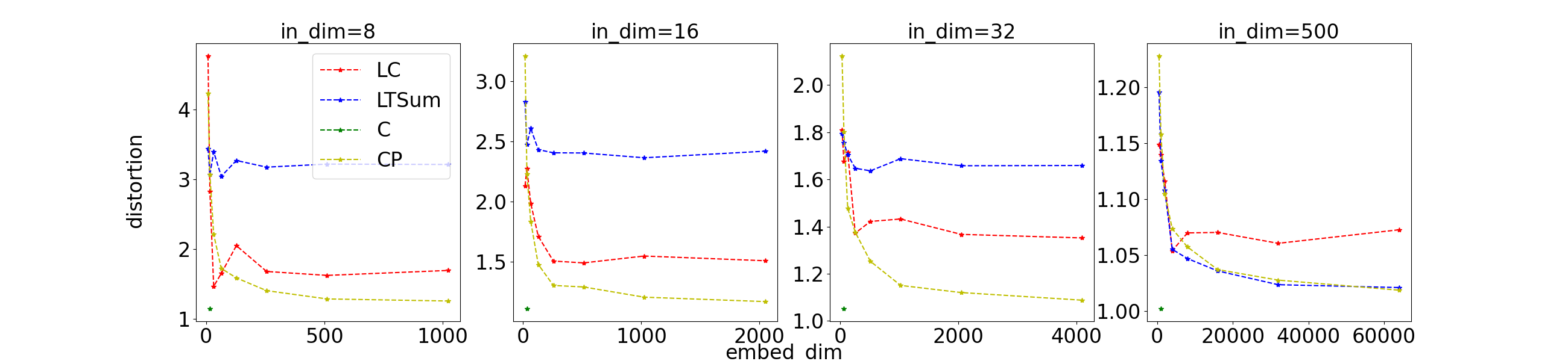
Figure 5: Distortion of the 2-tuple embeddings as a function of input and embedding dimension. LC=linear combination, LTSum=linear transform and sum, CP=concat project, C=concatenation.

Proof of Theorem D.1.

Linear combination: Let $x,z\in\mathbb{R}^{k},y,w\in\mathbb{R}^{l}$ We begin by proving that $f$ is lower Lipschitz continuous in expectation.

$$\mathbb{E}_{\alpha\sim U[-D,D]}[||f(x,y;\alpha)-f(z,w;\alpha)||_{p}^{p}]=\mathbb{E}_{\alpha\sim U[-D,D]}[||(\alpha\cdot x+y)-(\alpha\cdot w+z)||_{p}^{p}]$$

$$=\mathbb{E}_{\alpha\sim U[-D,D]}[||\alpha\cdot(x-z)+(y-w)||_{p}^{p}]$$

From equivalence of $l_{p}$ norms on finite dimensional spaces, $\exists c_{1}$ s.t.

$$\geq c_{1}\cdot\mathbb{E}_{\alpha\sim U[-D,D]}[||\alpha\cdot(x-z)+(y-w)||_{1}^{p}]$$

$$\stackrel{{\scriptstyle\text{Jensen's ineq.}}}{{\geq}}c_{1}\cdot\mathbb{E}_{\alpha\sim U[-D,D]}[||\alpha\cdot(x-z)+(y-w)||_{1}]^{p}$$

$$=c_{1}\cdot{E}_{\alpha\sim U[-D,D]}[||\alpha\cdot(x-z)||_{1}+||(y-w)||_{1}]^{p}$$

From equivalence of $l_{p}$ norms on finite dimensional spaces, $\exists c_{2}$ s.t.

$$\geq c_{1}\cdot c_{2}\cdot({E}_{\alpha\sim U[-D,D]}[|\alpha|]\cdot||(x-z)||_{p}+||(y-w)||_{p})^{p}$$

$$=c_{1}\cdot c_{2}\cdot(\frac{D}{2}\cdot||(x-z)||_{p}+||(y-w)||_{p})^{p}$$

$$\geq c_{1}\cdot c_{2}\cdot min(1,\frac{D}{2}^{p})\cdot(||(x-z)||_{p}+||(y-w)||_{p})^{p}$$

For uniform upper Lipschitz continuous bounds we have

$$||f(x,y;\alpha)-f(z,w;\alpha)||_{p} =||(\alpha\cdot x+y)-(\alpha\cdot w+z)||_{p}$$

$$\leq\|\alpha\cdot x-\alpha\cdot w\|_{p}+\|y-z\|_{p}$$

$$\leq\mathrm{max}(1,D)^{p}\cdot(||(x-z)||_{p}+||(y-w)||_{p})$$

Linear transform and sum: We prove lower-Lipschitz continuity n expectation. Let $a_{i}$ denote the i’th row of $A$. Recall that for any $1\leq i\leq l$, $a_{i}$ is drawn uniformly from $S^{k-1}$. Let $x,z\in\mathbb{R}^{k},y,w\in\mathbb{R}^{l}$

$$\mathbb{E}_{A}[||f(x,y;A)-f(z,w;A)||_{p}^{p}]=\mathbb{E}_{A}[||A(x-z)+(y-w)||_{p}^{p}]$$

$$=\mathbb{E}_{A}[\sum_{i=1}^{l}|\langle a_{i},x-z\rangle|^{p}+\sum_{j=1}^{l}|y_{j}-w_{j}|^{p}]=\sum_{i=1}^{l}\mathbb{E}_{a_{i}\sim S^{k-1}}[|\langle a_{i},x-z\rangle|^{p}]+\sum_{j=1}^{l}|y_{j}-w_{j}|^{p}$$

From lemma C.1 $\exists b>0$ s.t.

$$\mathbb{E}_{A}[||f(x,y;A)-f(z,w;A)||_{p}^{p}] \geq n\cdot b\cdot||x-z||_{p}^{p}+||y-w||_{p}^{p}$$

Let us denote $t=\begin{bmatrix}||x-z||_{p}\\ ||y-w||_{p}\end{bmatrix}\in\mathbb{R}^{2}$. Then

$$n\cdot b\cdot||x-z||_{p}^{p}+||y-w||_{p}^{p}\geq min(1,n\cdot b)\cdot(||x-z||_{p}^{p}+||y-w||_{p}^{p})=min(1,n\cdot b)\cdot||t||_{p}^{p}$$

From equivalence of norms on finite dimensional spaces, $\exists c>0$

$$\geq min(1,n\cdot b)\cdot c\cdot||t||_{1}^{p}=min(1,n\cdot b)\cdot c\cdot(||x-z||_{p}+||y-w||_{p})^{p}$$

Uniform upper Lipschitz continuity is straightforward to prove.

Concatenation: We show that this non-parametric function is bi-Lipschitz. Let $x,z\in\mathbb{R}^{k},y,w\in\mathbb{R}^{l}$. Denote as before $t=\begin{bmatrix}||x-z||_{p}\\ ||y-w||_{p}\end{bmatrix}\in\mathbb{R}^{2}$. Then the distance difference in the output space is given by $||f(x,y)-f(z,w)||_{p}^{p}=\|t\|_{p}$, while the difference in the input space is given by

$$\|x-z\|_{p}+\|y-w\|_{p}=\|t\|_{1}.$$

The claim follows from equivalence of $p$ norm and $1$ norm on $\mathbb{R}^{2}$.

Concat and project: The claim follows from the fact that the concatenation operation is bi-Lipschitz, and Lemma C.1. ∎

Appendix E Tree Mover’s Distance

In this appendix section we review the definition of the Tree Mover’s Distance (TMD) from [14], which is the way we measures distances between graphs in this paper.

We first review Wasserstein distances. Recall that if $(X,D)$ is a metric space, $\Omega\subseteq X$ is a subset, and $z$ is some point in $X$ with $dist(z,\Omega)>0$, then we can define the Wasserstein distance on the space of multisets consisting of $n$ elements in $\Omega$ via

$${W}_{1}(\{\!\!\{x_{1},\ldots,x_{n}\}\!\!\},\{\!\!\{y_{1},\ldots,y_{n}\}\!\!\})=\min_{\tau\in S_{n}}\sum_{j=1}^{n}D(x_{j},y_{\tau(j)})$$

The augmentation map on multisets of size $r\leq n$ is defined as

$$\rho_{(z)}\left(\{\!\!\{x_{1},\ldots,x_{r}\}\!\!\}\right)=\{\!\!\{x_{1},\ldots,x_{r},x_{r+1}=z,\ldots.x_{n}=z\}\!\!\}$$

and the augmented distance on multisets of size up to $n$ is defined via

$$W_{D,1}^{z}(X,\hat{X})=W_{D,1}(\rho_{(z)}X,\rho_{(z)}\hat{X})$$

We now return to define the TMD. We consider the space of graphs $G_{\leq n}(\Omega)$, consisting of graphs with $\leq n$ nodes, with node features coming from a compact domain $\Omega\subseteq\mathbb{R}^{d}$. We also fix some $z\in\mathbb{R}^{d}\setminus\Omega$. The TMD is defined using the notion of computation trees:

Definition E.1.

(Computation Trees). Given a graph $G=(V,E)$ with node features $\{\!\!\{x_{v}\}\!\!\}_{v\in V}$, let $T_{v}^{1}$ be the rooted tree with a single node $v$, which is also the root of the tree, and node features $x_{v}$. For $K\in\mathbb{N}$ let $T_{v}^{K}$ be the depth-$K$ computation tree of node $v$ constructed by connecting the neighbors of the leaf nodes of $T_{v}^{K-1}$ to the tree. Each node is assigned the same node feature it had in the original graph $G$. The multiset of depth-$K$ computation trees defined by $G$ is denoted by $\mathcal{T}_{G}^{K}:=\{\!\!\{T_{v}^{K}\}\!\!\}_{v\in V}$. Additionally, for a tree $T$ with root $r$, we denote by $\mathcal{T}_{r}$ the multiset of subtrees that root at the descendants of $r$.

Definition E.2.

(Blank Tree). A blank tree $\bar{T}_{z}$ is a tree (graph) that contains a single node and no edge, where the node feature is the blank vector $z$.

Recall that by assumption, all node features will come from the compact set $\Omega$, and $z\not\in\Omega$.

We can now define the tree distance:

Definition E.3.

(Tree Distance). The distance between two trees $T_{a},T_{b}$ with features from $\Omega$ and $z\not\in\Omega$, is defined recursively as

$$TD(T_{a},T_{b}):=\begin{cases}\|x_{r_{a}}-x_{r_{b}}\|_{p}+W_{TD,1}^{\bar{T}_{z}}(\mathcal{T}_{r_{a}},\mathcal{T}_{r_{b}})&\text{if $K>1$}\\ \|x_{r_{a}}-x_{r_{b}}\|_{p}&\text{otherwise}\end{cases}$$

where $K$ denotes the maximal depth of the trees $T_{a}$ and $T_{b}$.

Definition E.4.

(Tree Mover’s Distance). Given two graphs, $G_{a},G_{b}$ and $w,K\geq 0$, the tree mover’s distance is defined as

$$TMD^{K}(G_{a},G_{b})=W^{\bar{T}_{z}}_{TD,1}(\mathcal{T}_{G_{a}}^{K},\mathcal{T}_{G_{b}}^{K})$$

where $\mathcal{T}_{G_{a}}^{K}$ and $\mathcal{T}_{G_{b}}^{K}$ denote the multiset of all depth $K$ computational trees arising from the graphs $G_{a}$ and $G_{b}$, respectively. We refer the reader to [14] where they prove this is a pseudo-metric that fails to distinguish only graphs which cannot be separated by $K+1$ iterations of the WL test.

Appendix F MPNN Hölder theorem

In the main text we informally stated the following theorem

*

We will now give a formal statement of this theorem. The formal theorem also takes into account the node embeddings. We begin with some preliminary definitions.

Definition F.1.

(k-Partial MPNN). Given a MPNN $f$ with $K$, we denote the output of the first $k\leq K$ message passing layers:

$$f_{<k>}:=\psi^{(k)}\circ\phi^{(k)}\circ\ldots\circ\psi^{(1)}\circ\phi^{(1)}$$

as the k-partial MPNN. We define $f_{<0>}$ to be the identity function, and we denote the embedding of a specific node after $k$ message passing layers by $v\in V_{G}$ by $f_{<k>}(G)_{v}$

We will say that an MPNN $f:G_{\leq n}(\Omega)\times W\to\mathbb{R}^{m}$ is continuous, if for every fixed graph $G=(V,E)$ with $r\leq n$ nodes, and every number of iterations $k\leq K$, the functions

$$\Omega^{r}\times W\ni(X,w)\mapsto f_{<k>}\left((V,E,X);w\right)$$

$$\Omega^{r}\times W\ni(X,w)\mapsto f\left((V,E,X);w\right)$$

are continuous.

We denote by $\Omega_{k}$ the image of $f_{<k>}$ on graphs from $G_{\leq n}(\Omega)$ for every choice of parameters. Since the parameter domain and $\Omega$ are compact, assuming $f_{<k>}$ is continuous, $\Omega_{k}$ is also compact.

Theorem F.2.

(Hölder MPNN embeddings, full version) Let $p\geq 1$ and $K\in\mathbb{N}$, Let $f:G_{\leq n}(\Omega)\rightarrow\mathbb{R}^{m}$ be a continuous MPNN with $K$ message passing layers, defined by parametric functions $\phi^{(k)},\psi^{(k)},\eta$. Assume that $\Omega=\Omega_{0}$ is compact, and that for every choice of parameters of the MPNN, the features $x_{v}^{(k)}$ all reside in a compact set $\Omega_{k}$. Let $z_{k}\not\in\Omega_{k}$ be some point. Assume that the following assumptions hold for all $1\leq k\leq K$:

1. The aggregation, $\phi^{(k)}$, is $\alpha_{k}$ lower-Hölder continuous in expectation, and uniformly upper Lipschitz, w.r.t. the augmented Wasserstein distance $W_{1}^{z_{k}}$ on $\mathcal{S}_{\leq n}(\Omega_{k})$.

2. The combine function $\psi^{(k)}$, is $\beta_{k}$ lower-Hölder continuous in expectation, and uniformly upper Lipschitz.

3. the readout function $\eta$, is $\gamma$ lower-Hölder continuous in expectation, and uniformly upper Lipschitz, w.r.t. the augmented Wasserstein distance $W_{1}^{z_{K+1}}$ on $\mathcal{S}_{\leq n}(\Omega_{K+1})$..

where $\alpha_{k},\beta_{k},\gamma\geq 1$. Then,

1. The node embeddings are uniformly upper Lipschitz w.r.t. $TD$ on their depth $k+1$ computation trees. Moreover, they are lower-Hölder continuous in expectation, with the exponents being a product of the aggregate and combine exponents $\prod_{k=1}^{K}\alpha_{k}\cdot\beta_{k}$.

2. The graph embeddings are uniformly upper Lipschitz w.r.t. $TMD^{K+1}$. Moreover, they are lower-Hölder continuous in expectation , with the exponents being a product of the aggregate, combine and readout exponents. $\gamma\cdot\prod_{k=1}^{K}\alpha_{k}\cdot\beta_{k}$.

We now prove Theorem F.2. We state only the rather involved proof of lower-Hölder continuity in expectation, since the proof of the uniform upper Lipschitz bound is similar, and simpler.

In the proof, we will use the following notation.

Given a graph $G=(V,E)$, and a subset of nodes $U\subseteq V$ we denote by $f_{<k>}(U)$ the outputs of the k-partial MPNN for nodes in $U$: $\bigcup_{u\in U}f_{<k>}(G)_{u}$.

$\rho_{<k>}$ denotes augmentation using the output of the k-partial MPNN on the blank tree $\rho_{(f_{<k>}(\bar{T}_{z}))}$ and $\mathcal{T}_{v}^{K}$ denotes the depth-K computation trees of v’s neighbors: $\{T_{u}^{K}|u\in\mathcal{N}_{v}\}$.

We begin by proving a lemma that will assist us in the main proof

Lemma F.3.

Let $\Omega\subseteq\mathbb{R}^{d}$ be a compact set. Let $f:G_{\leq n}(\Omega)\rightarrow\mathbb{R}^{m}$ be a continuous function with $K$ message passing layers followed by a $READOUT$ layer. Assume that $x\not\in\Omega_{k}$. Then for any $G\in G_{\leq n}(\Omega),v\in V_{G}$ and for any $p\geq 1$, there exist $C\geq c>0$ such that

$$C\cdot TD(T_{v}^{k},\bar{T}_{z})\geq||x-f_{<k>}(G)_{v}||_{p}\geq c\cdot TD(T_{v}^{k},\bar{T}_{z})$$

Proof.

Since $f$ is continuous and $\Omega$ is compact, we get that $\Omega_{k}$ is compact. Therefore

$$a:=\inf_{y\notin\Omega_{k}}||x-y||_{p}>0$$

$$d:=\sup_{y\notin\Omega_{k}}||x-y||_{p}<\infty$$

Additionally, since $\Omega$ is compact and $z\not\in\Omega$, we can show recursively, starting from $k=1$, that for all $k\in\{0\ldots,K\}$ and all trees $T_{v}^{k}\in\mathcal{T}^{k}_{G_{\leq n}(\Omega)}$,

$$b:=\inf_{T_{v}^{k}\in\mathcal{T}^{k}_{G_{\leq n}(\Omega)}}TD(\bar{T}_{z},T_{v}^{k})>0$$

$$e:=\sup_{T_{v}^{k}\in\mathcal{T}^{k}_{G_{\leq n}(\Omega)}}TD(\bar{T}_{z},T_{v}^{k})<\infty$$

Where $\mathcal{T}^{k}_{G_{\leq n}(\Omega)}$ denotes the set of all possible height-$k$ computation trees from $G_{\leq n}(\Omega)$. Therefore, $\forall G\in G_{\leq n}(\Omega),v\in V_{G}$:

$$\frac{d}{b}\cdot TD(\bar{T}_{z},T_{v}^{k})\geq d\cdot\frac{b}{b}=d\geq||x-f_{<k>}(G)_{v}||_{p}\geq a=a\cdot\frac{e}{e}\geq\frac{a}{e}\cdot TD(\bar{T}_{z},T_{v}^{k})$$

To conclude we define $C:=\frac{d}{b},c:=\frac{a}{e}$.

∎

We will also use the well known property of norm equivalence on finite dimensional normed spaces (which we have already used many times previously)

Lemma F.4.

Let $p,q>0$ and $V$ be a finite dimensional normed space. There exist $C\geq c>0$ s.t. for any $v\in V$

$$C\cdot\|v\|_{q}\geq\|v\|_{p}\geq c\cdot\|v\|_{q}$$

In particular, this means that

Lemma F.5.

Let $p,q>0$ and $\Omega$ be a finite dimensional normed space. There exist $C\geq c>0$ s.t. for any $X,Y\in\mathcal{(}S)_{\leq n}\Omega$

$$C\cdot W_{q}^{z}(X,Y)\geq W_{p}^{z}(X,Y)\geq c\cdot W_{q}^{z}(X,Y)$$

Proof.

$$W_{p}^{z}(X,Y) =\left\{\min_{\tau\in S_{n}}\sum_{j=1}^{n}\|\rho_{(z)}(x)_{j}-\rho_{(z)}(y)_{\tau(j)}\|_{p}^{p}\right\}^{1/p}$$

$$\stackrel{{\scriptstyle\ref{norm_equiv}}}{{\geq}}c_{p1}\cdot\left\{\min_{\tau\in S_{n}}\sum_{j=1}^{n}\|\rho_{(z)}(x)_{j}-\rho_{(z)}(y)_{\tau(j)}\|_{p}\right\}$$

$$\stackrel{{\scriptstyle\ref{norm_equiv}}}{{\geq}}c_{p1}\cdot c_{pq}\cdot\left\{\min_{\tau\in S_{n}}\sum_{j=1}^{n}\|\rho_{(z)}(x)_{j}-\rho_{(z)}(y)_{\tau(j)}\|_{q}\right\}$$

$$\stackrel{{\scriptstyle\ref{norm_equiv}}}{{\geq}}c_{p1}\cdot c_{pq}\cdot c_{q1}\cdot\left\{\min_{\tau\in S_{n}}\sum_{j=1}^{n}\|\rho_{(z)}(x)_{j}-\rho_{(z)}(y)_{\tau(j)}\|_{q}^{q}\right\}^{\frac{1}{q}}$$

$$=c_{p1}\cdot c_{pq}\cdot c_{q1}\cdot W_{q}^{z}(X,Y)$$

The upper bound can be proven in the same manner. ∎

Proof of Theorem F.2.

Throughout the proof, we denote the k’th layer aggregation as $\phi^{(k)}$ with parameters $w\sim\mu_{k}$ and combine as $\psi^{(k)}$ with parameters $v\sim\lambda_{k}$. When discussing the parameters of multiple message passing layers, we will denote their parameters by $\theta_{k}:=(w_{1},\ldots,w_{k},v_{1},\ldots,v_{l})$ and the respective distributions by $\delta_{k}=(\mu_{1},\ldots,\mu_{k},\lambda_{1},\ldots,\lambda_{k})$. The readout layer will be denoted as $\eta$ with parameters $y\sim\sigma$. We will also use the notation $c_{g}$ to denote the positive lower-Hölder constant of a function and $\hat{c}=min(1,c)$.

We know that from $\Omega$’s compactness, $\exists D\geq d>0$ s.t. for any $x,y\in\Omega$ $d\leq\|x-y\|\leq D$. For simplicity we will assume throughout the proof that $\|x-y\|\leq 1$ (the proof can be written for the general case by adding a multiplicative fixing factor to the Hölder bounds).

Let $G=(V_{G},E_{G},X_{G}),H=(V_{H},E_{H},X_{H})\in G_{\leq n}(\Omega)$. We begin by proving the lower bound for the node embeddings by induction on $k$.

Let $v\in V_{G},u\in V_{H}$
Base
For $k=1$ we have that

$$\mathbb{E}_{\theta_{1}\sim\delta}[||f_{<1>}(G;\theta_{1})_{v}-f_{<1>}(H;\theta_{1})_{u}||_{p}^{p}]$$

$$=\mathbb{E}_{w\sim\mu_{1}}\mathbb{E}_{v\sim\lambda_{1}}[||\psi^{(1)}(x_{v},\phi^{(1)}(f_{<0>}(\mathcal{N}_{v});w);v)-\psi^{(1)}(x_{u},\phi^{(1)}(f_{<0>}(\mathcal{N}_{u});w);v)||_{p}^{p}]$$

$$\geq c_{\psi^{(1)}}\cdot\mathbb{E}_{w\sim\mu_{1}}[(||x_{v}-x_{u}||_{p}+||\phi^{(1)}(f_{<0>}(\mathcal{N}_{v});w)-\phi^{(1)}(f_{<0>}(\mathcal{N}_{u});w)||_{p})^{p\cdot\beta_{1}}]$$

$$\stackrel{{\scriptstyle\ref{norm_equiv}}}{{\geq}}c\cdot c_{\psi^{(1)}}\cdot(||x_{v}-x_{u}||_{p}^{p\cdot\beta_{1}}+\mathbb{E}_{w\sim\mu_{1}}[||\phi^{(1)}(f_{<0>}(\mathcal{N}_{v});w)-\phi^{(1)}(f_{<0>}(\mathcal{N}_{u});w)||_{p}^{p\cdot\beta_{1}}])$$

$$\stackrel{{\scriptstyle\text{Jensens ineq.}}}{{\geq}}c\cdot c_{\psi^{(1)}}\cdot(||x_{v}-x_{u}||_{p}^{p\cdot\beta_{1}}+\mathbb{E}_{w\sim\mu_{1}}[||\phi^{(1)}(f_{<0>}(\mathcal{N}_{v});w)-\phi^{(1)}(f_{<0>}(\mathcal{N}_{u});w)||_{p}^{p}]^{\beta_{1}}$$

$$\geq c\cdot c_{\psi^{(1)}}\cdot(||x_{v}-x_{u}||_{p}^{p\cdot\beta_{1}}+c_{\phi^{(1)}}\cdot W_{p}^{z}(f_{<0>}(\mathcal{N}_{v}),f_{<0>}(\mathcal{N}_{u}))^{p\cdot\alpha_{1}\cdot\beta_{1}})$$

$$\stackrel{{\scriptstyle\text{$p\cdot\alpha_{1}\cdot\beta_{1}\geq 1$}}}{{\geq}}c\cdot\hat{c}_{\phi^{(1)}}\cdot c_{\psi^{(1)}}\cdot(||x_{v}-x_{u}||_{p}^{p\cdot\alpha_{1}\cdot\beta_{1}}+W_{p}^{z}(f_{<0>}(\mathcal{N}_{v}),f_{<0>}(\mathcal{N}_{u}))^{p\cdot\alpha_{1}\cdot\beta_{1}})$$

for some $z\notin f_{<0>}(G_{\leq n}(\Omega))$

$$\stackrel{{\scriptstyle\ref{wass_equiv}}}{{\geq}}c_{w}\cdot c\cdot\hat{c}_{\phi^{(1)}}\cdot c_{\psi^{(1)}}\cdot(||x_{v}-x_{u}||_{p}^{p\cdot\alpha_{1}\cdot\beta_{1}}+W_{1}^{z}(f_{<0>}(\mathcal{N}_{v}),f_{<0>}(\mathcal{N}_{u}))^{p\cdot\alpha_{1}\cdot\beta_{1}})$$

Since $f_{<0>}$ is the identity, and since depth 1 computation trees with a single node (the root) are in fact vectors for which $TD=l_{p}$

$$=c_{w}\cdot c\cdot\hat{c}_{\phi^{(1)}}\cdot c_{\psi^{(1)}}\cdot(||x_{v}-x_{u}||_{p}^{p\cdot\alpha_{1}\cdot\beta_{1}}+W_{TD,1}^{\bar{T}_{z}}(\mathcal{T}_{v}^{1},\mathcal{T}_{u}^{1})^{p\cdot\alpha_{1}\cdot\beta_{1}})$$

$$\stackrel{{\scriptstyle\ref{norm_equiv}}}{{\geq}}c_{1}\cdot c_{w}\cdot c\cdot\hat{c}_{\phi^{(1)}}\cdot c_{\psi^{(1)}}\cdot(||x_{v}-x_{u}||_{p}+W_{TD,1}^{\bar{T}_{z}}(\mathcal{T}_{v}^{1},\mathcal{T}_{u}^{1}))^{p\cdot\alpha_{1}\cdot\beta_{1}}$$

$$=c\cdot TD(T_{v}^{2},T_{u}^{2})$$

for $c=c_{1}\cdot c_{w}\cdot c\cdot\hat{c}_{\phi^{(1)}}\cdot c_{\psi^{(1)}}$

Induction step
Assuming correctness for $k-1$, we will now prove correctness for $k$

$$\mathbb{E}_{\theta_{k}\sim\delta}[||f_{<k>}(G;\theta_{k})_{v}-f_{<k>}(H;\theta_{k})_{u}||_{p}^{p}]$$

$$=\mathbb{E}_{\theta_{k-1}\sim\delta_{k-1}}\mathbb{E}_{w\sim\mu_{k}}\mathbb{E}_{v\sim_{k}}[||\psi^{(k)}(f_{<k-1>}(G;\theta_{k-1})_{v},\phi^{(k)}(f_{<k-1>}(\mathcal{N}_{v};\theta_{k-1});w);v)$$

$$-\psi^{(k)}(f_{<k-1>}(G;\theta_{k-1})_{u},\phi^{(k)}(f_{<k-1>}(\mathcal{N}_{u};\theta_{k-1});w);v)||_{p}^{p}]$$

$$\geq c_{\psi^{(k)}}\cdot\mathbb{E}_{\theta_{k-1}\sim\delta_{k-1}}\mathbb{E}_{w\sim\mu_{k}}[(||f_{<k-1>}(G;\theta_{k-1})_{v}-f_{<k-1>}(G;\theta_{k-1})_{u}||_{p}$$

$$+||\phi^{(k)}(f_{<k-1>}(\mathcal{N}_{v};\theta_{k-1});w)-\phi^{(k)}(f_{<k-1>}(\mathcal{N}_{u};\theta_{k-1});w)||_{p})^{p\cdot\beta_{k}}]$$

$$\stackrel{{\scriptstyle\ref{norm_equiv}}}{{\geq}}c_{1}\cdot c_{\psi^{(k)}}\cdot\mathbb{E}_{\theta_{k-1}\sim\delta_{k-1}}\mathbb{E}_{w\sim\mu_{k}}[(||f_{<k-1>}(G;\theta_{k-1})_{v}-f_{<k-1>}(G;\theta_{k-1})_{u}||_{p}^{p\cdot\beta_{k}}$$

$$+||\phi^{(1)}(f_{<k-1>}(\mathcal{N}_{v};\theta_{k-1});w)-\phi^{(k)}(f_{<k-1>}(\mathcal{N}_{u};\theta_{k-1});w)||_{p}^{p\cdot\beta_{k}}])$$

$$\stackrel{{\scriptstyle\text{Jensens ineq.}}}{{\geq}}c_{1}\cdot c_{\psi^{(k)}}\cdot(\mathbb{E}_{\theta_{k-1}\sim\delta_{k-1}}[||f_{<k-1>}(G;\theta_{k-1})_{v}-f_{<k-1>}(G;\theta_{k-1})_{u}||_{p}^{p}]^{\beta_{k}}$$

$$+\mathbb{E}_{\theta_{k-1}\sim\delta_{k-1}}\mathbb{E}_{w\sim\mu_{k}}[||\phi^{(k)}(f_{<k-1>}(\mathcal{N}_{v};\theta_{k-1});w)-\phi^{(k)}(f_{<k-1>}(\mathcal{N}_{u};\theta_{k-1});w)||_{p}^{p}]^{\beta_{k}}$$

$$\geq c_{1}\cdot c_{\psi^{(k)}}\cdot(\mathbb{E}_{\theta_{k-1}\sim\delta_{k-1}}[||f_{<k-1>}(G;\theta_{k-1})_{v}-f_{<k-1>}(G;\theta_{k-1})_{u}||_{p}^{p}]^{\beta_{k}}$$

$$+c_{\phi^{(k)}}\cdot\mathbb{E}_{\theta_{k-1}\sim\delta_{k-1}}[W_{p}^{z_{k-1}}(f_{<k-1>}(\mathcal{N}_{v};\theta_{k-1}),f_{<k-1>}(\mathcal{N}_{u};\theta_{k-1}))^{p}]^{\alpha_{k}\cdot\beta_{k}})$$

for some $z_{k-1}\notin f_{<k-1>}(G_{\leq n}(\Omega))$

$$\geq c_{1}\cdot\hat{c}_{\phi^{(k)}}\cdot c_{\psi^{(k)}}\cdot(\mathbb{E}_{\theta_{k-1}\sim\delta_{k-1}}[||f_{<k-1>}(G;\theta_{k-1})_{v}-f_{<k-1>}(G;\theta_{k-1})_{u}||_{p}^{p}]^{\beta_{k}}$$

$$+\mathbb{E}_{\theta_{k-1}\sim\delta_{k-1}}[(\min_{\pi\in s_{n}}\sum_{i}||\rho_{(z_{k-1})}(f_{<k-1>}(\mathcal{N}_{v};\theta_{k-1}))_{i}-$$

$$\rho_{(z_{k-1})}(f_{<k-1>}(\mathcal{N}_{u};\theta_{k-1}))_{\pi^{-1}(i)}||_{p})^{p}]^{\alpha_{k}\cdot\beta_{k}})$$

$$\stackrel{{\scriptstyle\ref{norm_equiv}+\text{linearity}}}{{\geq}}c_{1}\cdot c_{2}\cdot\hat{c}_{\phi^{(k)}}\cdot c_{\psi^{(k)}}\cdot(\mathbb{E}_{\theta_{k-1}\sim\delta_{k-1}}[||f_{<k-1>}(G;\theta_{k-1})_{v}-f_{<k-1>}(G;\theta_{k-1})_{u}||_{p}^{p}]^{\beta_{k}}$$

$$+(\min_{\pi\in s_{n}}\sum_{i}\mathbb{E}_{\theta_{k-1}\sim\delta_{k-1}}[||\rho_{(z_{k-1})}(f_{<k-1>}(\mathcal{N}_{v};\theta_{k-1}))_{i}$$

$$-\rho_{(z_{k-1})}(f_{<k-1>}(\mathcal{N}_{u};\theta_{k-1}))_{\pi^{-1}(i)}||_{p}^{p}]^{\alpha_{k}\cdot\beta_{k}}))$$

We denote

$$\hat{\pi}:=arg\min_{\pi\in s_{n}}\sum_{i}\mathbb{E}_{\theta_{k-1}}[||\rho_{(z_{k-1})}(f_{<k-1>}(\mathcal{N}_{v};\theta_{k-1}))_{i}-\rho_{(z_{k-1})}(f_{<k-1>}(\mathcal{N}_{u};\theta_{k-1}))_{\pi^{-1}(i)}||^{p}]$$

$$\stackrel{{\scriptstyle\text{ind. hypothesis+\ref{lemma: blank_label inv.}}}}{{\geq}}c_{1}\cdot c_{2}\cdot\hat{c}_{\phi^{(k)}}\cdot c_{\psi^{(k)}}\cdot c_{k-1}\cdot((||x_{v}-x_{u}||_{p}+W_{TD}^{(\bar{T}_{z})}(\mathcal{T}_{v}^{k-1},\mathcal{T}_{u}^{k-1}))^{p\cdot\beta_{k}\cdot\prod_{l=1}^{k-1}\alpha_{l}\cdot\beta_{l}}$$

$$+(\sum_{i}\hat{c}TD(\rho_{(\bar{T}_{z})}(\mathcal{T}^{k}_{v})_{i},\rho_{(\bar{T}_{z})}(\mathcal{T}^{k}_{u})_{\hat{\pi}^{-1}(i)})^{p\cdot\prod_{l=1}^{k-1}\alpha_{l}\cdot\beta_{l}})^{\alpha_{k}\cdot\beta_{k}})$$

where $\hat{c}$ is the minimum of $1$ and the constant from F.3

$$\stackrel{{\scriptstyle\text{monotonicty}}}{{\geq}}\hat{c}\cdot c_{1}\cdot c_{2}\cdot\hat{c}_{\phi^{(k)}}\cdot c_{\psi^{(k)}}\cdot c_{k-1}\cdot((||x_{v}-x_{u}||_{p})^{p\cdot\beta_{k}\cdot\prod_{l=1}^{k-1}\alpha_{l}\cdot\beta_{l}}$$

$$+(\sum_{i}TD(\rho(\mathcal{T}^{k}_{v})_{i},\rho(\mathcal{T}^{k}_{u})_{\hat{\pi}^{-1}(i)})^{p\cdot\prod_{l=1}^{k-1}\alpha_{l}\cdot\beta_{l}})^{\alpha_{k}\cdot\beta_{k}})$$

$$\stackrel{{\scriptstyle\ref{norm_equiv}}}{{\geq}}\hat{c}\cdot c_{1}\cdot c_{2}\cdot c_{3}\cdot\hat{c}_{\phi^{(k)}}\cdot c_{\psi^{(k)}}\cdot c_{k-1}\cdot((||x_{v}-x_{u}||_{p})^{p\cdot\beta_{k}\cdot\prod_{l=1}^{k-1}\alpha_{l}\cdot\beta_{l}}$$

$$+(\sum_{i}TD(\rho(\mathcal{T}^{k}_{v})_{i},\rho(\mathcal{T}^{k}_{u})_{\hat{\pi}^{-1}(i)}))^{p\cdot\prod_{l=1}^{k}\alpha_{l}\cdot\beta_{l}}$$

$$\stackrel{{\scriptstyle||x_{v}-x_{u}||_{p}\leq 1}}{{\geq}}\hat{c}\cdot c_{1}\cdot c_{2}\cdot c_{3}\cdot\hat{c}_{\phi^{(k)}}\cdot c_{\psi^{(k)}}\cdot c_{k-1}\cdot((||x_{v}-x_{u}||_{p})^{p\cdot\beta_{k}\cdot\prod_{l=1}^{k}\alpha_{l}\cdot\beta_{l}}$$

$$+(\sum_{i}TD(\rho(\mathcal{T}^{k}_{v})_{i},\rho(\mathcal{T}^{k}_{u})_{\hat{\pi}^{-1}(i)}))^{p\cdot\prod_{l=1}^{k}\alpha_{l}\cdot\beta_{l}}$$

$$\stackrel{{\scriptstyle\ref{norm_equiv}}}{{\geq}}\hat{c}\cdot c_{1}\cdot c_{2}\cdot c_{3}\cdot c_{4}\cdot\hat{c}_{\phi^{(k)}}\cdot c_{\psi^{(k)}}\cdot c_{k-1}\cdot(||x_{v}-x_{u}||_{p}$$

$$+\sum_{i}TD(\rho(\mathcal{T}^{k}_{v})_{i},\rho(\mathcal{T}^{k}_{u})_{\hat{\pi}^{-1}(i)}))^{p\cdot\prod_{l=1}^{k}\alpha_{l}\cdot\beta_{l}}$$

$$=c_{k}\cdot TD(T_{v}^{k+1},T_{u}^{t+1})$$

for $c_{k}=\hat{c}\cdot c_{1}\cdot c_{2}\cdot c_{3}\cdot c_{4}\cdot\hat{c}_{\phi^{(k)}}\cdot c_{\psi^{(k)}}\cdot c_{k-1}$ concluding the proof for the expected lower-Hölder bound for node embeddings.

For the expected lower-Hölder bound of graph embeddings:

$$\mathbb{E}_{(y,\theta_{K})\sim(\sigma,\delta)}[||f(G;\theta_{K},y)-f(H;\theta_{K},y)||_{p}^{p}]$$

$$\stackrel{{\scriptstyle x\notin f_{<K>}(G_{\leq n}(\Omega))}}{{\geq}}\mathbb{E}_{\theta_{K}\sim\delta}[c_{\eta}\cdot W^{x}_{1}(f_{<K>}(G;\theta_{K}),f_{<K>}(H;\theta_{K}))^{\gamma\cdot p}]$$

Denoting $\pi^{*}:=arg\min_{\pi\in P}\sum_{i}||\rho_{(x)}(f_{<K>}(G;\theta_{K}))_{i}-\rho_{(x)}(f_{<K>}(H;\theta_{K}))_{\pi(i)}||$

$$\stackrel{{\scriptstyle\text{Jensen ineq.}}}{{\geq}}c_{\eta}\cdot\mathbb{E}_{\theta_{K}\sim\delta}(\sum_{i}\mathbb{E}_{\theta_{K}\sim\delta}[||\rho_{(x)}(f_{<K>}(G;\theta_{K}))_{i}-\rho_{(x)}(f_{<K>}(H;\theta_{K}))_{\pi^{*}(i)}||_{p}^{p}])^{\gamma}$$

using F.3 for distance between MPNN outputs and augmentation labels, and what we already proved for node embeddings

$$\geq c_{\eta}\cdot c_{K}\cdot(\sum_{i}TD(\rho_{(\bar{T}_{z})}(\mathcal{T}_{G}^{K+1})_{i},\rho_{(\bar{T}_{z})}(\mathcal{T}_{H}^{K+1})_{\pi^{*}(i)})^{p\cdot\prod_{l=1}^{K}\alpha_{l}\cdot\beta_{l}})^{\gamma}$$

$$\stackrel{{\scriptstyle\ref{norm_equiv}}}{{\geq}}c\cdot c_{\eta}\cdot c_{K}\cdot(\sum_{i}TD(\rho_{(\bar{T}_{z})}(\mathcal{T}_{G}^{K+1})_{i},\rho_{(\bar{T}_{z})}(\mathcal{T}_{H}^{K+1})_{\pi^{*}(i)}))^{\gamma\cdot p\cdot\prod_{l=1}^{K}\alpha_{l}\cdot\beta_{l}}$$

$$=c_{K+1}\cdot W^{\bar{T}_{z}}_{TD,1}(\mathcal{T}^{K+1}_{G},\mathcal{T}^{K+1}_{H})$$

for $c_{K+1}=c\cdot c_{\eta}\cdot c_{K}$ concluding the proof for lower-Hölder bounds. ∎

Appendix G Upper bounds for explicit MPNN constructions

In the main text we stated the following corollary of Theorem F.2: * To make this corollary formal, we need to specify the distribution on the parameters used. Basically, we just use the distributions used to guarantee Hölder continuity for the various components. There are two cases in which more care is needed.

For ReluMPNN, since our theorem on ReLU summation requires the bias to be larger than the norm of all features, so the parameter distribution at each depth $k$ needs to be chosen so that this requirement is fulfilled.

Similarly, for SortMPNN, to use our theorem on sort-based multiset functions we need to use at each iteration $k$ the operation $\rho_{(z_{k})}$ with a vector $z_{k}$ which is not a feature in the space $\Omega_{k}$ of possible features $x_{v}^{(k)}$. We note that a choice of such $z_{k}$ exists since we assume that all parameters, and all features at initialization, come from a compact set, which ensures that all features throughout the construction will be bounded.

This leads to the following corollary (for simplicity we state the corollary for MPNN with width 1. Similar statements can be easily made for general width $W$ , by independenly drawning the same parameters for all $W$ independent instances.

Corollary G.1.

1. SortMPNN with $K$ iterations is uniformly Lipschitz, and lower Lipschitz in expectation, with respect to $TMD^{K}$, where the vectors $a_{i}^{(k)},b_{i}^{(k)}$ and the rows of the matrices used for the combine step are drawn uniformly from the unit circle, and the augmentation vector $z_{k}$ is chosen so that it cannot be attained as a $k$ generation feature of the network.

2. AdaptMPNN with $K$ iterations is uniformly Lipschitz, and $[(p+1)/p]^{K+1}$ lower Hölder in expectation, where all parameters $t_{k}\sim[0,1]$, and all other parameters are drawn uniformly from the unit circle.

3. ReLUMPNN with $K$ iterations is uniformly Lipschitz, and $[(p+1)/p]^{K+1}$ lower Hölder in expectation, where bias parameters $b\sim[-B_{k},B_{k}]$ with $B_{k}$ larger than the maximal norm of all possible features of generation $k$, and all other parameters are drawn uniformly from the unit circle.

Appendix H Lower bounds for MPNN exponents via $\epsilon$ trees

In the main text of the paper we stated the following informal theorem * We note that the distribution on the parameters taken in this theorem is the same as described throughout the text. The aggregation used for both MPNNs at hand is of the form

$$\{\!\!\{x_{1},\ldots,x_{s}\}\!\!\}\mapsto\sum_{i=1}^{s}\rho(a\cdot x_{i}-b)$$

where $a$ and $b$ are drawn uniformly from the unit sphere and some interval $[-B,B]$ respectively. Of course, in ReluMPNN $\rho=\mathrm{ReLU}$ while with smoothMPNN $\rho$ is a smooth function. The parameters of the linear COMBINE function are also selected uniformly in the unit sphere.

$\epsilon$-Tree dataset

The proof of the theorem is based on a family of adversarial example which we denote by $\epsilon$-trees. The recursive construction depends on two parameters: a real number $\epsilon$, and an integer $T=0,1,\ldots$. This will give us a pair of trees $(G,\hat{G})$ where $G=G(T,\epsilon),\hat{G}=\hat{G}(T,\epsilon)$.

The recursive construction of $\epsilon$ trees is depicted in Figure 6. In the first step $T=0$, we define ’trees’ $a_{0},b_{0},c_{0},d_{0}$ which consist of a single node, with feature value of $\epsilon,-\epsilon,2\epsilon$ and $-2\epsilon$, respectively. We connect $a_{0},b_{0}$ via a new root with feature value $0$ to create the tree $G_{0}=G(T=0,\epsilon)$, as depicted in the left hand side of Figure 6. We do the same thing with $c_{0},d_{0}$ to obtain the tree $\hat{G}_{0}=\hat{G}(T=0,\epsilon)$.

We now proceed recursively, again as shown in Figure 6. Assuming that for a given $T$ we have defined the trees $a_{T},b_{T},c_{T},d_{T},G_{T},\hat{G}_{T}$, we define the corresponding trees for $T+1$ as shown in the figure:

For example, $a_{T+1}$ is constructed by joining together two copies of $a_{T}$ and two copies of $b_{T}$ at a common root with feature value $0$ as shown in the figure on the right hand side. From the figure one can also infer the construction of $b_{T+1},c_{T+1},d_{T+1}$ from $a_{T},b_{T},c_{T},c_{T}$. Finally, the tree $G_{T+1}$ is constructed by joining together $c_{T+1},d_{T+1}$ while $\hat{G}_{T+1}$ is constructed by joining together $a_{T+1},b_{T+1}$

Proof of Theorem 4.2.

Denoting an MPNN of depth $T$ by $f_{T}(G,w)$, where $w$ denotes the network’s parameters, our goal is to provide bounds of the form

$$\mathbb{E}_{w}\|f_{T}(G(T,\epsilon),w)-f_{T}(\hat{G}(T,\epsilon),w)\|^{p}\leq C\epsilon^{p\beta}$$ (7)

where $\beta$ depends on $T$ and the activation used, and on the other had show that $TMD^{T}(G(T,\epsilon),\hat{G}(T,\epsilon))$ scales linearly in $\epsilon$. This will prove that the MPNN cannot be $\alpha$-lower Hölder with any $\alpha<\beta$.

We can see that $TMD^{T}(G(T,\epsilon),\hat{G}(T,\epsilon))$ scales linearly in $\epsilon$ because the TMD is homogenous. Namely, given any $G=(V,E,X)$ and $\epsilon>0$, let $\epsilon G=(V,E,\epsilon X)$. Then for any $T$ we have

$$TMD^{T}(\epsilon G,\epsilon\hat{G})=\epsilon\cdot TMD^{T}(G,\hat{G}).$$

We now turn to estimate the exponent $\beta$ in (7), for smooth or ReLU activations, and different values of $T$. To avoid cluttered notation we will explain what occurs for low values $T=0$ and $T=1$ in detail, and outline the argument for larger $T$.

When $T=0$, we apply an MPNN of depth $T=0$ to the graphs $G_{0},\hat{G}_{0}$, which means that we just apply a readout function to the initial features. This is exactly the $\pm\epsilon$ example discussed in the main text, and so (7) will hold with $\beta=(p+1)/p$ with ReLU activations, and $\beta=2$ with smooth activations.

We now consider the case $T=1$. Here we apply we an MPNN of depth $T=1$ to the graphs $G_{1},\hat{G}_{1}$. Let us denote the nodes of $G_{1}$ by $V_{1}$, using the natural correspondence defined by the figure (middle) we can think of $V_{1}$ as the nodes of $\hat{G}_{1}$ as well. We denote the node feature values at node $v$ after a single MPNN iteration by $x_{v,w}$ and $\hat{x}_{v,w}$, where $w$ denotes the network parameters as before.

Note that for the root $r$ we have that $x_{r,w}=\hat{x}_{r,w}$ for any choice of parameters $w$.

At initialization, all leaves of the trees $G_{0},G_{1}$ are assigned one of the values $\epsilon,-\epsilon,2\epsilon,-2\epsilon$ (according to the labeling $a_{0},b_{0},c_{0}$ or $d_{0}$). If two leaves are assigned the same value (both are denoted by, say, $a_{0}$), then they will have the same node feature after a single message passing iteration, since they are only connected to their father, and all fathers have the same initial node feature.

We now consider the two remaining nodes. We denote the node connected to the root from the left by $v_{1}$ and the node connected to the root from the right by $v_{2}$.

Let us first focus on the smooth activation case. We note that the children of $v_{1}$ and $v_{2}$, in both graphs, have initial features of order $\epsilon$, and the all sum to the same value zero. By considering the Taylor approximation of the activation, as discussed in the proof of Theorem 1, we see that for an appropriate constant $C$ we have that for all small enough $\epsilon$,

$$|c_{v,w}-\hat{c}_{u,w}|\leq C\epsilon^{2},\text{ for all parameters }w$$ (8)

where $v$ and $u$ could either be $v_{1}$ or $v_{2}$, and we recall that $c_{v,w}$ is the output of the aggregation function, applied to the initial features of the neighbors of $v$ in $G$ (and $\hat{c}_{u,w}$ is defined analogously for the neighbors of $u$ in $\hat{G}$).

Additionally, we note that for every parameter $w$ we have that

$$c_{v_{1},w}+c_{v_{2},w}=2\left[\psi_{w}(\epsilon)+\psi_{w}(-\epsilon)+\psi_{w}(2\epsilon)+\psi_{w}(-2\epsilon)\right]=\hat{c}_{v_{1},w}+\hat{c}_{v_{2},w}$$ (9)

where $\psi_{w}$ denotes the neural network used for aggregation. The next step in the MPNN procedure is the COMBINE step, after which we will have a bound of the form (9), namely

$$|x_{v,w}-\hat{x}_{u,w}|\leq C\epsilon^{2},\text{ for all parameters }w$$ (10)

since the COMBINE functions we use are uniformly Lipschitz, and we will also have or every parameter $w$ we have that

$$x_{v_{1},w}+x_{v_{2},w}=\hat{x}_{v_{1},w}+\hat{x}_{v_{2},w}$$ (11)

since our COMBINE function is linear.

Now, when applying the readout function, we have eleven node features in the multiset of nodes of $G_{1}$ and $\hat{G}_{1}$. For any parameter vector $w$, if we remove the nodes $v_{1},v_{2}$, we get two identical multisets. Therefore, we only need to bound the difference

$$\|\left[\eta_{w}(x_{v_{1},w})+\eta_{w}(x_{v_{2},w})\right]-\left[\eta_{w}(\hat{x}_{v_{1},w})+\eta_{w}(\hat{x}_{v_{2},w}\right]\|$$

Since by (11) the features sum to the same value, and all are the same up to $\epsilon^{2}$, this difference goes like $\epsilon^{4}$. This is what we wanted. For general $T$, we will be able to apply this same argument recursively $T+1$ times to get the lower bound of $2^{T+1}$ for the smooth exponent.

Now, let us consider what happens when we replace the smooth activation with ReLU activation. In This case too, the only features which really matter are those corresponding to $v_{1},v_{2}$. Recalling our analysis of the $\pm\epsilon$ for ReLU activations, we note that if the bias of the network falls outside the interval $[-2\epsilon,2\epsilon]$, then all node features $x_{v_{1},w},x_{v_{2},w},\hat{x}_{v_{2},w},\hat{x}_{v_{2},w}$ will all be identical. If the bias does fall in that interval, then the difference between these node features can be bounded from above by $C\epsilon$ for an appropriate constant $C$. When applying readout, there is a probability of $\sim\epsilon^{2}$ that the final global features will be distinct (if the parameters of aggregation, and the parameters of readout, are both well behaved). The difference in this case can again be bounded by $C\epsilon$. It follows that

$$\mathbb{E}_{w}\|f_{T}(G(T,\epsilon),w)-f_{T}(\hat{G}(T,\epsilon),w)\|^{p}\leq C\epsilon^{2}\epsilon^{p}$$

which will lead to a lower bound on the Hölder constant $\alpha\geq(1+\frac{2}{p})$.

For general $T$, we will get that there is a probability of $\sim\epsilon^{T+1}$ to obtain any separation, and that, if this separation occurs, the difference between features will be $\leq C\cdot\epsilon$. As a result, the expectation

$$\mathbb{E}_{w}\|f_{T}(G(T,\epsilon),w)-f_{T}(\hat{G}(T,\epsilon),w)\|^{p}$$

will scale like $\epsilon^{T+1+p}$, which leads to our lower bound on the exponent for ReLU activations. ∎

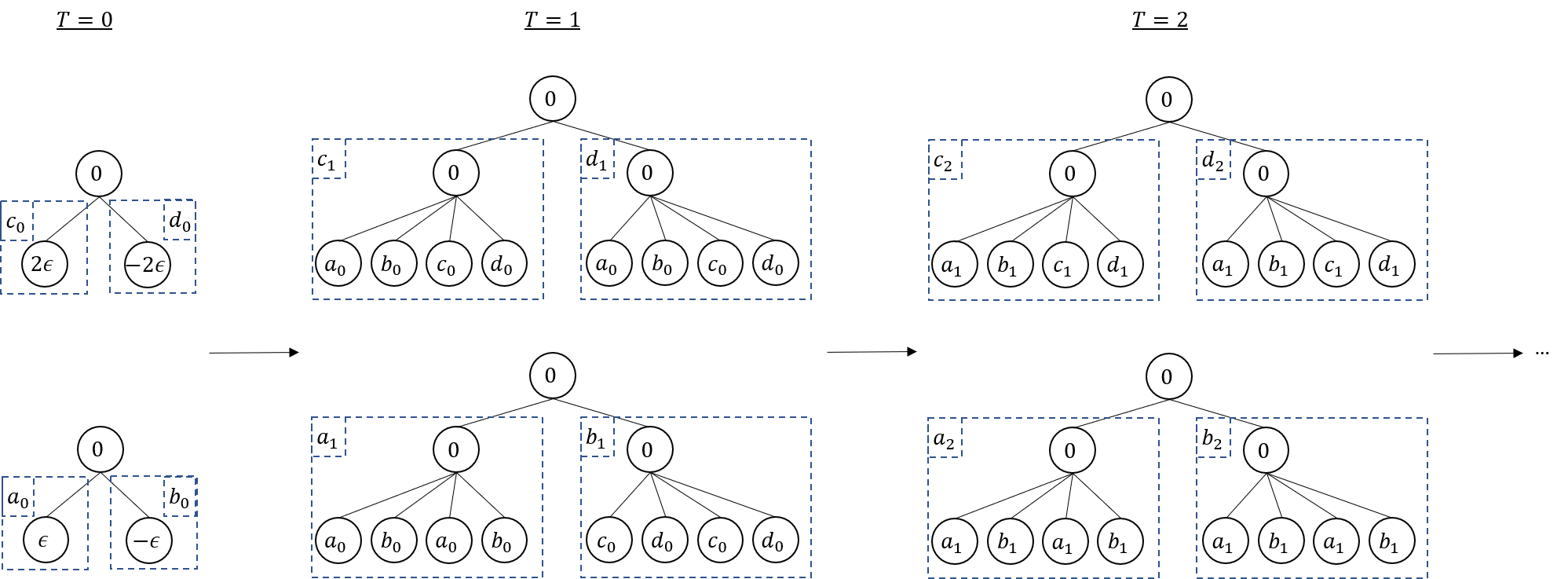
Figure 6: $\epsilon$-tree dataset construction: The trees are built using basic elements $a_{t},b_{t},c_{t},d_{t}$. At step $T$, the basic elements are defined using subtrees from the previous step.

Appendix I Experiments

I.1 Hardware

All experiments were executed on an a cluster of 8 nvidia A40 49GB GPUs.

I.2 Architecture variations

In this subsection we will lay out the architectural variations that were considered for SortMPNN and AdaptMPNN, that were omitted from the main text for brevity. We include explanations of these variations with the connection between them and the theoretical analysis.

SortMPNN

First off, we must choose how to model of the blank vector, since SortMPNN uses the blank vector explicitly in (2). We propose three options for the (blank method):

1. Learnable: For every multiset aggregation function there is a unique learnable blank vector that is used for augmentation. Since we assume the node features are from a compact subset of $\mathbb{R}^{d}$, there exist valid augmentation vectors, and upon training we can expect the learnable vector to converge to a valid augmentation vector. Note that this method assumes training takes place.

2. Iterative update: In this method, the blank vector of each layer is the output of the previous MPNN layers on the blank tree, where the blank tree node feature is set to zero. This works under two assumptions: (1): The nodes in the dataset don’t have the feature zero. (2): The intermediate layer outputs on computation trees from the data don’t clash with the same layer output on the blank tree. This seems relatively reasonable since SortMPNN is bi-Lipschitz in expectation, which in expectation should lead to injectivity.

3. Zero: simply using the zero vector as the blank vector. This works under the assumption that the zero vector is neither a valid initial feature, nor a valid output of intermediate layers. This is the weakest of the three, but was experimented with nonetheless.

Given a multiset $X$, we experimented with two variations for the aggregation implementation. Both share step (1), but differ in step (2):

1. projection: $X\mapsto colsort(A\rho_{(z)}(X)):=Y\in\mathbb{R}^{m\times n}$, where $A\in\mathbb{R}^{m\times d}$.

2. collapse: In this step, we either perform (1) a matrix collapse: $rowsum(B\odot Y)$ where $\odot$ is the element-wise product and $B\in\mathbb{R}^{m\times n}$ or (2) a vector collapse: $Yb$, for $b\in\mathbb{R}^{n}$.

Note that when choosing to use the matrix collapse, under the assumption that the blank method provides a valid blank vector, this is equivalent to running $m$ separate copies of $S_{z}$ (2) with independent parameters (at least upon initialization), just like we proposed in the main text. When using the vector collapse, the aggregation takes the form of multiple instances of $S_{z}$ except that that the parameter $b$ used in the inner product is shared across instances. Note the Hölder expectation doesn’t change in this case, but the variance is likely higher. We explored this option since it reduces the number of parameters needed for the aggregation, potentially easing the optimization process.

In addition, we experimented with adding bias to the projection, and to the vector collapse.

AdaptMPNN

The main detail we left out from the main text is the fact that the output of $m_{\mathrm{ReLU}}^{\mathrm{adapt}}$ is in $\mathbb{R}^{4}$, whereas we would want it to be in $\mathbb{R}$ in order to be able to stack $m$ instances and get an output in $\mathbb{R}^{d}$. In order to get the desired output dimension, we compose $m_{\mathrm{ReLU}}^{\mathrm{adapt}}$ with a projection, and the aggregation on a multiset $X\in\mathbb{R}^{d\times r}$ as follows:

1. Stacked Adaptive ReLU:

   $$Y:=\begin{bmatrix}m_{\mathrm{ReLU}}^{\mathrm{adapt}}(X;a_{1},t_{1})\\ \vdots\\ m_{\mathrm{ReLU}}^{\mathrm{adapt}}(X;a_{m},t_{m})\end{bmatrix}\in\mathbb{R}^{m\times 4}$$

2. Project: $rowsum(B\odot Y)$ where $\odot$ is the element-wise product and $B\in\mathbb{R}^{m\times 4}$ has rows that are drawn uniformly independently from $S^{3}$.

As we proved previously C.1, an inner product with a vector drawn uniformly from $S^{d-1}$ is bi-Hölder in expectation. From composition properties B.1, this means that the above stacking of multiple independent instances of $project\circ m_{\mathrm{ReLU}}^{\mathrm{adapt}}$ keeps the Hölder properties of $m_{\mathrm{ReLU}}^{\mathrm{adapt}}$.

In addition, we experimented with four optional changes to the aggregation:

1. Adding the sum $\sum\langle x_{j},a\rangle$ a 5’th coordinate to the output of $m_{\mathrm{ReLU}}^{\mathrm{adapt}}$. The idea behind this choice is that the sum is an informative feature which is encountered when using the standard ReLU activations and bias smaller than the minimal feature in the multiset. For adaptive ReLU, this summation will only occur when $t=0$.

2. Note that the adaptive relu uses the parameter $t\in[0,1]$ to choose a bias within the minimal and maximal multiset values. When training, we experimented with either clamping $t$ to $[0,1]$ or otherwise lifting this constraint.

3. We experimented with adding a bias term to the projection step, since this can potentially lead to stronger expressivity.

4. the initialization of $t$ was optionally chosen to be linspace between $[0,1]$.

I.3 $\epsilon$-tree dataset

Distortion experiment

The experiment depicted in 2 was run on a set of $1,000$ pairs of trees with $\epsilon$ going from $0.05$ to $0.4$. The first $500$ trees are of height $h=3$ and were input to MPNNs of depth $d=1$, and the other $500$ trees were of height $h=4$ and were input to MPNNs of depth $d=2$. The plots in figure 2 were separated by MPNN depth in order for the phenomenon to be clearly visible. We note that the feature of all non-leaf nodes which appear with $0$ in figure 6, was set to be $1$. All the models in the experiment used linear combination as the combine function, had an embedding dimension of $45,000$, except SortMPNN that used an embedding dimension of $2,048$ due to resource constraints. The large width was used to show the behavior of the MPNNs as we approach the expected value over the parameters. In order to plot the curve in each subplot, the minimal ratio $r_{min}=l_{2}/TMD^{\alpha}$ was computed for each graph pair where $\alpha$ is the theoretical lower-Hölder exponent. Then, $r_{min}\cdot x^{\alpha}$ was plotted. Note that $r_{min}$ was only computed for half of the pairs with the largest TMD values in order to avoid the case where the embedding distance is zero leading to $r_{min}=0$.

Throughout the experiment, double precision was used in order to capture the small differences as needed. The measured embedding distance was taken over the output of the readout function, without further processing.

Separation experiment

For the trained graph separation experiment, $100$ pairs of $\epsilon$ trees of height $h=4$ with $\epsilon\in[0.1,1]$ were used. Trees corresponding to the first row in figure 6 were given the label $0$, and trees from the second row were given the label $1$. The models were trained by inputting a single pair as a batch per training iteration. All models were composed of 2 message passing layers, followed by readout and a single linear layer to obtain a logit. All of $\{64,128,256,512\}$ were tested for the embedding dimension with results consistent regardless of the embedding dimension. The models were trained for 10 epochs using the adamw optimizer and a learning rate of 0.01.

I.4 TUDataset

Results on datasets that appear in table 3 for GIN, GCN, GraphSage are from [35], except for GIN on NCI109 which is from [14]. The reported results in 3 for the fully trained SortMPNN and AdaptMPNN were chosen out to be the best single result out of 30 random hyper-parameter choices from the following hyperparameters: batch size$\in\{32,64\}$, depth$\in[2-5]$, embed dim$\in\{16,32,64\}$, combine$\in\{ConcatProject,LinearCombination,LTSum\}$, dropout$\in\{0,0.1,0.2\}$,output mlp depth $\in\{1,2,3\}$, weight decay $\in\{0,0.01,0.1\}$, lr$\in[0.0001,0.01]$, optimizer $\in[adam,adamw]$, #epochs$=500$. In addition, for SortMPNN the blank method was taken to be iterative update, and the collapse method was taken to be from {matrix, vector} without bias begin used at any stage. For AdaptMPNN, adding the sum of the multiset was a hyper-parameter, as was the choice if to clamp the parameter $t$ to be in $[0,1]$. The choice of the 30 random configurations was chosen with wandb [5] sweeps.

As stated in the main text, results are reported as in [35]. Namely, we report the mean and standard deviation of the validation performance over stratified 10-folds, where the validation curves of all 10 folds are aggregated, and the best epoch is chosen.

I.5 LRGB

In both experiments from table 4, the models adhere to the 500K parameter limit. The hyper-parameters were tuned for a single seed, and then the configuration with the best validation results was rerun for 4 different seeds. We report the mean and standard deviation on the test set in table 2. The code from the official LRGB github repo was used to run these experiments, with the only change being the addition of our architectures. The reported results for other models are taken from [31].

peptides-func

For SortMPNN, the following hyper-parameters were used to achieve the results shown in the table 4: blank method - learnable, collapse method - vector, bias used both in projection and collapse, combine - ConcatProject, embedding dimension - 165, message passing layers - 4, final mlp layers - 3, dropout - 0.05, weight decay - 0.01, positional encoding - RWSE [16], learning rate - 0.005, scheduler - cosine with warmup, optimizer - adamW. Number of parameters: 494865.

For AdaptMPNN - the following hyper-parameters were used: the bias parameter $t$ was clamped to stay within $[0,1]$, the sum of a multiset was added as a 5’th coordinate, bias added in project, collapse method - LinearCombination, embedding dimension - 220, message passing layers - 6, final mlp layers - 3, dropout - 0.05,weight decay - 0.01, positional encoding - RWSE, learning rate - 0.001, scheduler - cosine with warmup, optimizer - adamW. Number of parameters: 480915.

peptides-struct

For SortMPNN: blank method - learnable, collapse method - matrix, bias not used both in projection or collapse, combine - LinearCombination, embedding dimension - 200, message passing layers - 6, final mlp layers - 3, dropout - 0, weight decay - 0.01, positional encoding - LapPE [15], learning rate - 0.005, scheduler - step, optimizer - adamW. Number of parameters: 493858.

For AdaptMPNN:the bias parameter $t$ was clamped to stay within $[0,1]$, the sum of a multiset was added as a 5’th coordinate, bias added in project, collapse method - LinearCombination, embedding dimension - 220, message passing layers - 6, final mlp layers - 3, dropout - 0,weight decay - 0.1, positional encoding - LapPE, learning rate - 0.001, scheduler - step, optimizer - adamW. Number of parameters: 480973.

small models

Additional experiments run on peptides struct were performed by running models with the exact same hyper-parameters aside from the width. Results are shown in figure 4. Exact width and number of parameters (including for the 500K budget) appear in table 5.

Budget	SortMPNN	AdaptMPNN	GCN
500K	[200 | 493.8K]	[220 | 478.8K]	[235 | 488K]
100K	[70 | 95.9K]	[95 | 98.6K]	[100 | 98.4K]
50K	[48 | 47.3]	[65 | 49.3K]	[68 | 48.8K]
25K	[34 | 24.9K]	[44 | 24.3K]	[46 | 24.2K]
7K	[17 | 6.7K]	[22 | 6.7K]	[23 | 6.8K]

Table 5: [width | #params] per model for each parameter budget

I.6 Subgraph aggregation networks

In this experiment, we made use of edge features. The incorporation of edge features was chosen to be one of two options: (1) simple sum of the node feature and the corresponding edge feature before computing the message to be sent to a node’s neighbor. (2) sum of the node feature and the corresponding edge feature, followed by the linear layer of the aggregation (this is the first step in the aggregation both in the sort based and adaptive relu aggragation) and finally a ReLU. This was tested since it is used in the GINE architecture [23]. We call the first w-relu, and the second wo-relu. Test set mean and standard deviation were computed over 10 random seeds. Hyper-parameters were chosen by randomly running 40 configurations with the DS edge deleted configuration, and choosing the best. the validation set was done using a single seed. The code provided with [4] was used to run these experiments, with the only change being the addition of our architectures.

SortMPNN

Both for the DS and DSS experiments, the model consisted of 5 message passing layers, used sum Jumping Knowledge (JK) from [36], Combine - ConcatProject, matrix collapse, bias was added to projection, blank method - learnable, edge features - wo-relu for DS and w-relu for DSS. The model was trained for 400 epochs with lr=0.01 and batch size of 128.

AdaptMPNN

Both for the DS and DSS experiments, the model consisted of 5 message passing layers, sum JK for DS and last for DSS, combine - ConcatProject, sum wasn’t added, $t$ was clapmed to $[0,1]$, bias was added throughout aggregation steps, edge features - wo-relu. The model was trained for 400 epochs, with lr of 0.005 for DS and 0.01 for DSS.

References

- [1] Tal Amir et al. “Neural Injective Functions for Multisets, Measures and Graphs via a Finite Witness Theorem” In Thirty-seventh Conference on Neural Information Processing Systems, 2023 URL: https://openreview.net/forum?id=TQlpqmCeMe
- [2] Radu Balan, Naveed Haghani and Maneesh Singh “Permutation invariant representations with applications to graph deep learning” In arXiv preprint arXiv:2203.07546, 2022
- [3] Radu Balan and Efstratios Tsoukanis “G-Invariant Representations using Coorbits: Bi-Lipschitz Properties”, 2023 arXiv:2308.11784 [math.RT]
- [4] Beatrice Bevilacqua et al. “Equivariant Subgraph Aggregation Networks” In The Tenth International Conference on Learning Representations, ICLR 2022, Virtual Event, April 25-29, 2022 OpenReview.net, 2022 URL: https://openreview.net/forum?id=dFbKQaRk15w
- [5] Lukas Biewald “Experiment Tracking with Weights and Biases” Software available from wandb.com, 2020 URL: https://www.wandb.com/
- [6] Jan Böker “Graph similarity and homomorphism densities” In arXiv preprint arXiv:2104.14213, 2021
- [7] Jan Böker et al. “Fine-grained Expressivity of Graph Neural Networks” In Thirty-seventh Conference on Neural Information Processing Systems, 2023 URL: https://openreview.net/forum?id=jt10uWlEbc
- [8] Fedor Borisyuk et al. “LiGNN: Graph Neural Networks at LinkedIn”, 2024 arXiv:2402.11139 [cs.LG]
- [9] César Bravo, Alexander Kozachinskiy and Cristóbal Rojas “On dimensionality of feature vectors in MPNNs” In arXiv preprint arXiv:2402.03966, 2024
- [10] Xavier Bresson and Thomas Laurent “Residual Gated Graph ConvNets”, 2018 arXiv:1711.07553 [cs.LG]
- [11] Jameson Cahill, Andres Contreras and Andres Contreras-Hip “Complete set of translation invariant measurements with Lipschitz bounds” In Applied and Computational Harmonic Analysis 49.2 Elsevier, 2020, pp. 521–539
- [12] Jameson Cahill, Joseph W. Iverson and Dustin G. Mixon “Towards a bilipschitz invariant theory”, 2024 arXiv:2305.17241 [math.FA]
- [13] Samantha Chen et al. “Weisfeiler-lehman meets gromov-Wasserstein” In International Conference on Machine Learning, 2022, pp. 3371–3416 PMLR
- [14] Ching-Yao Chuang and Stefanie Jegelka “Tree Mover’s Distance: Bridging Graph Metrics and Stability of Graph Neural Networks” In Advances in Neural Information Processing Systems, 2022 URL: https://openreview.net/forum?id=Qh89hwiP5ZR
- [15] Vijay Prakash Dwivedi and Xavier Bresson “A Generalization of Transformer Networks to Graphs” In AAAI Workshop on Deep Learning on Graphs: Methods and Applications, 2021
- [16] Vijay Prakash Dwivedi et al. “Graph Neural Networks with Learnable Structural and Positional Representations” In International Conference on Learning Representations, 2022 URL: https://openreview.net/forum?id=wTTjnvGphYj
- [17] Vijay Prakash Dwivedi et al. “Long Range Graph Benchmark” In Advances in Neural Information Processing Systems 35 Curran Associates, Inc., 2022, pp. 22326–22340 URL: https://proceedings.neurips.cc/paper_files/paper/2022/file/8c3c666820ea055a77726d66fc7d447f-Paper-Datasets_and_Benchmarks.pdf
- [18] Nadav Dym and Steven J. Gortler “Low Dimensional Invariant Embeddings for Universal Geometric Learning”, 2023 arXiv:2205.02956 [cs.LG]
- [19] Chen Gao et al. “A Survey of Graph Neural Networks for Recommender Systems: Challenges, Methods, and Directions”, 2023 arXiv:2109.12843 [cs.IR]
- [20] Justin Gilmer et al. “Neural Message Passing for Quantum Chemistry” In International Conference on Machine Learning, 2017 URL: https://api.semanticscholar.org/CorpusID:9665943
- [21] Martin Grohe “word2vec, node2vec, graph2vec, x2vec: Towards a theory of vector embeddings of structured data” In Proceedings of the 39th ACM SIGMOD-SIGACT-SIGAI Symposium on Principles of Database Systems, 2020, pp. 1–16
- [22] Will Hamilton, Zhitao Ying and Jure Leskovec “Inductive Representation Learning on Large Graphs” In Advances in Neural Information Processing Systems 30 Curran Associates, Inc., 2017 URL: https://proceedings.neurips.cc/paper_files/paper/2017/file/5dd9db5e033da9c6fb5ba83c7a7ebea9-Paper.pdf
- [23] Weihua Hu* et al. “Strategies for Pre-training Graph Neural Networks” In International Conference on Learning Representations, 2020 URL: https://openreview.net/forum?id=HJlWWJSFDH
- [24] Ningyuan Huang and Soledad Villar “A Short Tutorial on The Weisfeiler-Lehman Test And Its Variants” In ICASSP 2021 - 2021 IEEE International Conference on Acoustics, Speech and Signal Processing (ICASSP), 2021, pp. 8533–8537 URL: https://api.semanticscholar.org/CorpusID:235780517
- [25] Thomas N. Kipf and Max Welling “Semi-Supervised Classification with Graph Convolutional Networks” In International Conference on Learning Representations, 2017 URL: https://openreview.net/forum?id=SJU4ayYgl
- [26] Christopher Morris et al. “Future Directions in Foundations of Graph Machine Learning”, 2024 arXiv:2402.02287 [cs.LG]
- [27] Christopher Morris et al. “TUDataset: A collection of benchmark datasets for learning with graphs”, 2020 arXiv:2007.08663 [cs.LG]
- [28] Christopher Morris et al. “Weisfeiler and Leman Go Neural: Higher-Order Graph Neural Networks” In The Thirty-Third AAAI Conference on Artificial Intelligence, AAAI 2019, The Thirty-First Innovative Applications of Artificial Intelligence Conference, IAAI 2019, The Ninth AAAI Symposium on Educational Advances in Artificial Intelligence, EAAI 2019, Honolulu, Hawaii, USA, January 27 - February 1, 2019 AAAI Press, 2019, pp. 4602–4609 DOI: 10.1609/AAAI.V33I01.33014602
- [29] Kristof T. Schütt et al. “Quantum-chemical insights from deep tensor neural networks” In Nature Communications 8.1 Springer ScienceBusiness Media LLC, 2017 DOI: 10.1038/ncomms13890
- [30] Puoya Tabaghi and Yusu Wang “Universal Representation of Permutation-Invariant Functions on Vectors and Tensors” In Proceedings of The 35th International Conference on Algorithmic Learning Theory 237, Proceedings of Machine Learning Research PMLR, 2024, pp. 1134–1187 URL: https://proceedings.mlr.press/v237/tabaghi24a.html
- [31] Jan Tönshoff, Martin Ritzert, Eran Rosenbluth and Martin Grohe “Where Did the Gap Go? Reassessing the Long-Range Graph Benchmark”, 2023 arXiv:2309.00367 [cs.LG]
- [32] Petar Velickovic et al. “Graph Attention Networks” In 6th International Conference on Learning Representations, ICLR 2018, Vancouver, BC, Canada, April 30 - May 3, 2018, Conference Track Proceedings OpenReview.net, 2018 URL: https://openreview.net/forum?id=rJXMpikCZ
- [33] Edward Wagstaff et al. “On the Limitations of Representing Functions on Sets” In International Conference on Machine Learning, 2019 URL: https://api.semanticscholar.org/CorpusID:59292002
- [34] Boris Weisfeiler and AA Lehman “A reduction of a graph to a canonical form and an algebra arising during this reduction” In Nauchno-Technicheskaya Informatsia 2.9, 1968, pp. 12–16
- [35] Keyulu Xu, Weihua Hu, Jure Leskovec and Stefanie Jegelka “How Powerful are Graph Neural Networks?” In International Conference on Learning Representations, 2019 URL: https://openreview.net/forum?id=ryGs6iA5Km
- [36] Keyulu Xu et al. “Representation Learning on Graphs with Jumping Knowledge Networks” In Proceedings of the 35th International Conference on Machine Learning 80, Proceedings of Machine Learning Research PMLR, 2018, pp. 5453–5462 URL: https://proceedings.mlr.press/v80/xu18c.html
- [37] Manzil Zaheer et al. “Deep sets” In Advances in neural information processing systems 30, 2017
- [38] Muhan Zhang, Zhicheng Cui, Marion Neumann and Yixin Chen “An End-to-End Deep Learning Architecture for Graph Classification” In Proceedings of the Thirty-Second AAAI Conference on Artificial Intelligence, (AAAI-18), the 30th innovative Applications of Artificial Intelligence (IAAI-18), and the 8th AAAI Symposium on Educational Advances in Artificial Intelligence (EAAI-18), New Orleans, Louisiana, USA, February 2-7, 2018 AAAI Press, 2018, pp. 4438–4445 DOI: 10.1609/AAAI.V32I1.11782
- [39] Yan Zhang, Jonathon Hare and Adam Prügel-Bennett “FSPool: Learning Set Representations with Featurewise Sort Pooling”, 2019 URL: https://arxiv.org/abs/1906.02795