Motion Consistency Model:
Accelerating Video Diffusion with
Disentangled Motion-Appearance Distillation

Abstract

Image diffusion distillation achieves high-fidelity generation with very few sampling steps. However, applying these techniques directly to video diffusion often results in unsatisfactory frame quality due to the limited visual quality in public video datasets. This affects the performance of both teacher and student video diffusion models. Our study aims to improve video diffusion distillation while improving frame appearance using abundant high-quality image data. We propose motion consistency model (MCM), a single-stage video diffusion distillation method that disentangles motion and appearance learning. Specifically, MCM includes a video consistency model that distills motion from the video teacher model, and an image discriminator that enhances frame appearance to match high-quality image data. This combination presents two challenges: (1) conflicting frame learning objectives, as video distillation learns from low-quality video frames while the image discriminator targets high-quality images; and (2) training-inference discrepancies due to the differing quality of video samples used during training and inference. To address these challenges, we introduce disentangled motion distillation and mixed trajectory distillation. The former applies the distillation objective solely to the motion representation, while the latter mitigates training-inference discrepancies by mixing distillation trajectories from both the low- and high-quality video domains. Extensive experiments show that our MCM achieves the state-of-the-art video diffusion distillation performance. Additionally, our method can enhance frame quality in video diffusion models, producing frames with high aesthetic scores or specific styles without corresponding video data.

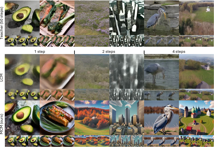
Figure 1: Qualitative result comparisons with latent consistency model (LCM) [38] using ModelScopeT2V [62] as teacher. Our MCM outputs clearer video frames using few-step sampling, and can also adapt to different image styles using additional image datasets. Corresponding video results are in supplementary materials.

1 Introduction

Diffusion models [22, 54, 42, 23, 28, 45] have significantly advanced the quality of text-to-image generation [45, 8, 13], enabling the creation of high-fidelity images and allowing for diverse stylistic variations [3, 2, 1]. The recent development in image diffusion distillation [55, 34, 48, 38, 31] significantly reduces the inference cost by letting distilled student models to perform high-fidelity generation with extremely low sampling steps.

Due to the additional temporal dimension, the sampling time for video diffusion models [21, 24, 9, 62, 19, 65] is considerably longer than that for image diffusion models. However, directly extending image distillation methods to speed up the video diffusion models results in unsatisfactory frame appearance quality. Specifically, unlike image diffusion models that benefit from high-quality image datasets such as LAION [49], public video datasets [70, 57, 5] often suffer from lower frame quality, including issues like low resolution, significant motion blur, and watermarks. This discrepancy poses a great challenge, as the quality of the training data directly impacts both the teacher generation quality and the distillation process. An example is shown in Fig. 1, where both the teacher and the latent consistency model (LCM) student [38, 66] learn the watermark from the video dataset.

To address this challenge, we propose motion consistency model (MCM), a single-stage video diffusion distillation method that enables few-step sampling and can optionally leverage a high-quality image dataset to improve the video frame quality. We showcase our results in Fig. 1 bottom row and Fig. 6, and illustrate the distillation process in Fig. 2.

To simultaneously achieve the goal of diffusion distillation and frame quality improvement, we build our method upon a video LCM [38, 66] combined with an image adversarial objective [47, 48], due to their proven effectiveness in the two tasks [38, 66, 61, 75, 27], respectively. However, directly combining them presents two essential problems. (1) Conflicted frame learning objectives. The LCM aims to learn and represent the characteristics of low-quality video frames, while the adversarial objective pushes the frames toward high-quality image data. This opposition creates conflicts between preserving low-quality visual features and enhancing image quality. (2) Discrepant training-inference distillation input. During training, only low-quality video samples are used for LCM distillation, whereas during inference, the input is generated high-quality video samples. These two problems greatly hinders the distillation process and the generated frame quality.

To address the first problem, we propose disentangled motion distillation. Specifically, we disentangle the motion components from the video latent, and only distill the motion knowledge from the teacher. Meanwhile, the image adversarial objective is used exclusively to learn frame appearance. This approach effectively mitigates the conflict between learning objectives by ensuring that motion and appearance are learned independently. For the second problem, we propose mixed trajectory distillation. We simulate the probability flow ordinary differential equation (PF-ODE) trajectory during inference and sample generated high-quality videos from this simulated trajectory for distillation. By mixing distillation between low-quality video samples and generated high-quality video samples, we ensure better alignment between training and inference phases, thereby enhancing overall performance.

In summary, our contributions are as follows:

• We propose motion consistency model (MCM), a single-stage video diffusion distillation method that accelerates the sampling process and can optionally leverage an image dataset to enhance the quality of generated video frames.

• We introduce disentangled motion distillation to resolve the conflicting frame learning objectives between video diffusion distillation and image adversarial learning, ensuring better motion consistency and frame appearance.

• We propose mixed trajectory distillation, which simulates the PF-ODE trajectory during inference. By combining low-quality video samples with generated high-quality video samples during distillation, our approach improves training-inference alignment and enhances generation quality.

• We conduct extensive experiments, demonstrating that our MCM significantly improves video diffusion distillation performance. Furthermore, when leveraging an additional image dataset, our MCM better aligns the appearance of the generated video with the high-quality image dataset.

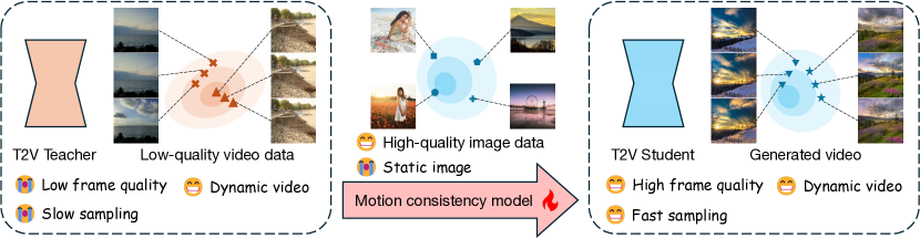
Figure 2: Illustration of our motion consistency model distillation process, which not only distills the motion prior from teacher to accelerate sampling, but also can benefit from an additional high-quality image dataset to improve the frame quality of generated videos.

2 Preliminaries

Diffusion models. Diffusion models [22] consists of a forward and a reverse process. The forward process corrupts the data progressively by interpolating a Gaussian noise $\bm{\epsilon}\in\mathcal{N}(0,\bm{I})$ and the data sample $\bm{x}_{0}$: $\bm{x}_{t}=q(\bm{x}_{0},\bm{\epsilon},t)=\alpha_{t}\bm{x}_{0}+\sigma_{t}\bm{\epsilon}$, where $\alpha_{t}$ and $\sigma_{t}$ are pre-defined noise schedule. The reverse process learns a time-conditioned model to gradually removes the noise. Recent methods [56, 37] propose to design numerical solvers of ordinary differential equations (ODE) to reduce the number of sampling steps.

Consistency model. Consistency model (CM) [55] is a new family of generative models that enables few-step sampling. The essence of CM $\bm{f}(\bm{x}_{t},t)$ is the self-consistency property, that maps any point in the same probability flow ODE (PF-ODE) trajectory to a same point. That is, $\bm{f}(\bm{x}_{t},t)=\bm{f}(\bm{x}_{t^{\prime}},t^{\prime})$ for $\forall t,t^{\prime}\in[\epsilon,T]$, where $\epsilon$ is a fixed small positive number. The boundary condition $\bm{f}(\bm{x}_{\epsilon},\epsilon)=\bm{x}_{\epsilon}$ ensures the CM always predicts the origin of PF-ODE trajectories. CM is parameterized as the weighted sum of the data sample and a model output $\bm{F}$ parameterized by $\theta$:

$$\bm{f}(\bm{x}_{t},t)=c_{\text{skip}}(t)\bm{x}_{t}+c_{\text{out}}(t)\bm{F}_{\theta}(\bm{x}_{t},t),$$ (1)

where $c_{\text{skip}}(t)$ and $c_{\text{out}}(t)$ are differentiable functions [55, 28] with $c_{\text{skip}}(\epsilon)=1$ and $c_{\text{out}}(\epsilon)=0$.

CM can be learned via consistency distillation (CD), where a teacher model $\phi$ and an ODE solver $\bm{\Phi}$ estimates the previous sample in the empirical PF-ODE trajectory, with $s$ being the step size:

$$\hat{\bm{x}}_{t-s}^{\phi}=\bm{x}_{t}-s\bm{\Phi}(\bm{x}_{t},t;\phi).$$ (2)

Let $\theta$ be the student model parameter, and its exponential moving average (EMA) $\theta^{-}\leftarrow\mu\theta^{-}+(1-\mu)\theta$ be the target model parameter. CD is trained to enforce the self-consistency property, which minimizes the distance between student and target outputs:

$$\mathcal{L}_{\text{CD}}=\mathbb{E}_{\bm{x}_{0},\bm{\epsilon},t}\left[d\left(\bm{f}_{\theta}(\bm{x}_{t},t),\bm{f}_{\theta^{-}}(\hat{\bm{x}}_{t-s}^{\phi},t-s)\right)\right].$$ (3)

In this paper, we follow previous methods [38, 61] to use Huber loss as the distance function: $d(\bm{x}_{t},\bm{x}_{t}^{\prime})=\sqrt{\|\bm{x}_{t}-\bm{x}_{t}^{\prime}\|^{2}_{2}+\delta^{2}}-\delta$, where $\delta$ is a threshold hyperparameter.

3 Motion consistency model

We present motion consistency model (MCM), a novel video diffusion distillation method designed for accelerating the text-to-video diffusion sampling process. Additionally, MCM can leverage a different image dataset to adjust the frame appearance, e.g., frame quality improvement, watermark removal or frame style transfer. An illustration of the objective is shown in Fig. 2.

Problem formulation. Given a pre-trained text-to-video diffusion model $\phi$, a video-caption dataset $\mathbb{V}=\{(\bm{v},c)_{i}\}$, and an image dataset $\mathbb{M}=\{m_{i}\}$, our objective is twofold.

1. Distill the motion knowledge from teacher $\phi$ into a student $\theta$ using the video dataset $\mathbb{V}$, enabling few-step video generation.

2. Adjust the appearance of the generated video frames using the image dataset $\mathbb{M}$.

In this paper, we assume that the appearance of video frames in $\mathbb{V}$ has lower quality compared to the images in $\mathbb{M}$. For convenience, we refer to the appearance of video frames as following a “low-quality” distribution and the images in $\mathbb{M}$ as following a “high-quality” distribution.

When the image dataset $\mathbb{M}$ consists of frames extracted from the video dataset $\mathbb{V}$, this task simplifies into a straightforward video diffusion distillation process.

3.1 Video latent consistency model meets image discriminator

A straightforward way to achieve the aforementioned goal is to adopt a two-stage training strategy [61], i.e., train a 2D backbone with the image dataset, and then temporally inflate the backbone to fine-tune temporal layers on videos. However, not only this approach can be time-consuming, but the disjointed training stages can lead to suboptimal motion modeling and degraded appearance learning. To address this problem, we propose a single-stage, end-to-end learnable approach.

To build a strong baseline, we adopt a video latent consistency model (LCM) [38] $\bm{f}_{\theta}(\cdot,\cdot)$ with a frame adversarial objective [47, 48]. The LCM has proven effective in diffusion distillation [38, 66, 61], and the adversarial objective has been widely used for style transfer [75, 27] and diffusion distillation [48]. By combining these two approaches, we aim to achieve both few-step sampling and improved frame appearance control.

For the discriminator $D(\cdot)$ used in the adversarial learning, we adopt a pixel-space discriminator following previous methods [47, 48]. However, densely applying the adversarial objective to all frames is computationally expensive, and can lead to degraded temporal smoothness [72]. To mitigate this, drawing inspiration from sparse sampling-based action recognition [52, 64, 63], we apply the adversarial loss only to a set of sparsely sampled frames.

Specifically, let $\hat{\bm{x}}_{0}^{\theta}=\bm{f}_{\theta}(\bm{x}_{t},t)$ represent the LCM-predicted video latent, and $\hat{\bm{v}}_{0}^{\theta}=\mathscr{D}(\hat{\bm{x}}_{0}^{\theta})$ be the decoded video, where $\mathscr{D}$ is the latent decoder. We randomly sample $l$ frames from the video, denoted as $\{\hat{v}_{0,0}^{\theta,\text{s}},...,\hat{v}_{0,l}^{\theta,\text{s}}\}$, and apply the adversarial loss to these sampled frames:

$$\mathcal{L}_{\text{adv}}^{\text{G}}=-\mathbb{E}_{\bm{x}_{0},\bm{\epsilon},t}\left[\frac{1}{l}\sum_{i}D_{\psi}(\hat{v}_{0,i}^{\theta,\text{s}})\right],$$ (4)

where $\psi$ is the learnable parameter in $D(\cdot)$. The discriminator is trained to minimize

$$\mathcal{L}_{\text{adv}}^{\text{D}}=\mathbb{E}_{\bm{x}_{0},\bm{\epsilon},t}\left[\max\left(0,1+\frac{1}{l}\sum_{i}D_{\psi}(\hat{v}_{0,i}^{\theta,\text{s}})\right)\right]+\mathbb{E}_{m_{i}}\left[\max(0,1-D_{\psi}\left(m_{i}\right))\right].$$ (5)

We omit the gradient penalty term [18, 48] for conciseness. Please find details on the discriminator design in [47, 48] or in Appendix C. Note that the discriminator’s objective is to distinguish between the generated video frame and the images from the image dataset $\mathbb{M}$, thereby aligning the video frame with the high-quality distribution.

The overall baseline learning objective is a weighted sum of the CD loss (Eq. 3) and the adversarial loss: $\mathcal{L}_{\text{base}}=\mathcal{L}_{\text{CD}}+\lambda_{\text{adv}}\mathcal{L}_{\text{adv}}^{\text{G}}$, where $\lambda_{\text{adv}}$ is the weighting hyperparameter.

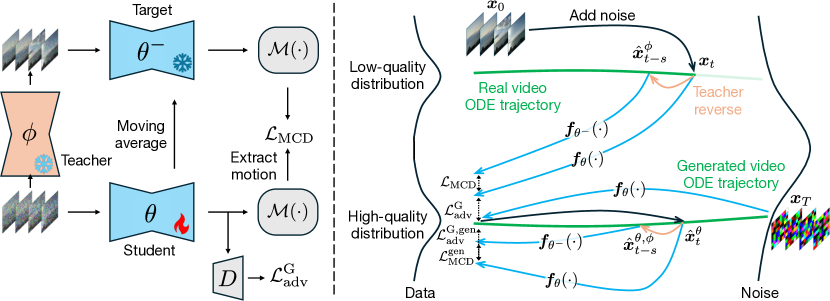
Figure 3: Left: framework overview. Our MCM features disentangled motion-appearance distillation, where motion is learned via the motion consistency distillation loss $\mathcal{L}_{\text{MCD}}$, and the appearance is learned with the frame adversarial objective $\mathcal{L}_{\text{adv}}^{\text{G}}$. Right: mixed trajectory distillation. We simulate the inference-time ODE trajectory using student-generated video (bottom green line), which is mixed with the real video ODE trajectory (top green line) for consistency distillation training.

3.2 Disentangled motion consistency distillation

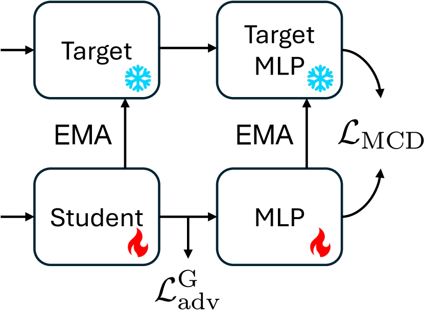
Figure 4: Learnable motion representation.

While combining LCM and the adversarial loss is straightforward, their training objectives conflict. The LCM aligns the appearance of the predicted video with the low-quality distribution, while the adversarial objective adjust the appearance to match the high-quality distribution. Moreover, as LCM relies solely on boundary conditions (Sec. 2) to generate clean video frames, it typically leads to blurry frame as $t$ approaches $T$ [55, 38, 61]. This blurriness conflicts with the adversarial loss objective, which seeks to produce clean frames at all steps.

To mitigate these conflicts, we propose a disentangled approach: separating the motion presentation from the video latent, and applying the LCM objective exclusively to the motion representation to ensure temporal smoothness. Meanwhile, we use the adversarial objective to learn the frame appearance. This disentanglement allows us to leverage the strengths of both objectives without them interfering with each other. An illustration is shown in Fig. 3 left.

Specifically, we replace the original consistency distillation loss $\mathcal{L}_{\text{CD}}$ in $\mathcal{L}_{\text{base}}$ with the following motion consistency distillation (MCD) objective $\mathcal{L}_{\text{MCD}}$:

$$\mathcal{L}_{\text{MCD}}=\mathbb{E}_{\bm{x}_{0},\bm{\epsilon},t}\left[d\left(\mathcal{M}\left(\bm{f}_{\theta}(\bm{x}_{t},t)\right),\mathcal{M}\left(\bm{f}_{\theta^{-}}(\hat{\bm{x}}_{t-s}^{\phi},t-s)\right)\right)\right],$$ (6)

where $\mathcal{M}(\cdot)$ indicates motion representation extraction function. In this paper, we consider the following implementations.

• Latent difference: the difference between temporally consecutive frame latents. This was used in action recognition [52, 64, 74] as motion representations.

• Latent correlation: a 4D cost volume tensor containing pairwise dot-product between consecutive frame latents, widely used in optical flow estimation [26, 51, 50].

• Latent low/high-frequency components: this is inspired by recent work [69], which shows different frequency components of the latent have different impacts on the motion.

• Learnable representation: we apply a two-layer MLP after the LCM output to extract motion (Fig. 4). This MLP does not contain temporal layers, and preserves the motion while avoiding direct applying appearance loss to the latent. The parameters of the target MLP head are updated using exponential moving average, and the MLP is discarded during inference. This design resembles the projection head used in self-supervised learning [17, 11, 12, 10].

We examine all choices in Sec. 4.3, and find that the learnable representation works the best.

3.3 Mixed trajectory distillation

While the disentangled motion distillation mitigates the appearance learning objective conflicts, another training-inference discrepancy persists. During training, all ODE trajectories used for MCD are sampled by adding noise to the low-quality videos in $\mathbb{V}$ (Fig. 3 top right). In contrast, during inference, the ODE trajectories will be sampled in the high-quality video space. As a result, such discrepancy leads to degraded performance during inference. Furthermore, since we do not have access to high-quality videos, we cannot directly sample ODE trajectories from this distribution for training, making it challenging to resolve this training-inference discrepancy.

To address this problem, we propose to simulate such high-quality video ODE trajectories by using the consistency model multi-step inference process [55]. Specifically, starting from random noise $\bm{x}_{T}\in\mathcal{N}(0,\bm{I})$, we first run single-step inference to get the high-quality data sample $\hat{\bm{x}}_{0}^{\theta}$, and then add noise to it to sample high-quality ODE trajectories. An illustration is shown in Fig. 3 bottom right. Formally, the starting point $\hat{\bm{x}}_{t}^{\theta}$ for MCD is sampled as:

$$\hat{\bm{x}}_{t}^{\theta}=\alpha_{t}\hat{\bm{x}}_{0}^{\theta}+\sigma_{t}\bm{\epsilon},\ \text{where}\ \hat{\bm{x}}_{0}^{\theta}=\bm{f}_{\theta}(\bm{x}_{T},T)\ \text{and}\ \bm{x}_{T}\in\mathcal{N}(0,\bm{I}).$$ (7)

In this way, the MCD loss can be formulated by replacing the starting data points from those sampled from low-quality trajectories with those sampled from simulated high-quality video trajectories:

$$\mathcal{L}_{\text{MCD}}^{\text{gen}}=\mathbb{E}_{\bm{x}_{T},\bm{\epsilon},t}\left[d\left(\mathcal{M}\left(\bm{f}_{\theta}(\hat{\bm{x}}_{t}^{\theta},t)\right),\mathcal{M}\left(\bm{f}_{\theta^{-}}(\hat{\bm{x}}_{t-s}^{\theta,\phi},t-s)\right)\right)\right],$$ (8)

where $\hat{\bm{x}}_{t-s}^{\theta,\phi}=\hat{\bm{x}}_{t}^{\theta}-s\bm{\Phi}(\hat{\bm{x}}_{t}^{\theta},t;\phi)$. Similarly, the adversarial loss is also applied to the model prediction from the samples on the high-quality trajectories, which we denote as $\mathcal{L}_{\text{adv}}^{\text{G},\text{gen}}$. By applying the MCD and adversarial objectives to the simulated high-quality trajectory, it not only mitigates the training-inference trajectory discrepancy, but also ensures zero terminal signal-to-noise ratio $\bm{x}_{T}\in\mathcal{N}(0,\bm{I})$ to avoid the data leakage problem [33] and helps plain video distillation.

In practice, we found that only training from the generated video ODE trajectory potentially leads to mode collapse (Sec. B.1), and mixing the training from real samples and generated samples achieves the best results. Thus, the final loss $\mathcal{L}$ is formulated as a weighted sum of the distillation objectives using real samples and generated samples:

$$\mathcal{L}=\lambda_{\text{real}}\left(\mathcal{L}_{\text{MCD}}+\lambda_{\text{adv}}\mathcal{L}_{\text{adv}}^{\text{G}}\right)+(1-\lambda_{\text{real}})\left(\mathcal{L}_{\text{MCD}}^{\text{gen}}+\lambda_{\text{adv}}\mathcal{L}_{\text{adv}}^{\text{G},\text{gen}}\right),$$ (9)

where $\lambda_{\text{real}}\in[0,1]$ is a hyperparameter to balance the distillation in different trajectories.

Table 1: Video diffusion distillation comparison on the WebVid mini validation set.

Teacher	Method	FVD@Step $\downarrow$				CLIPSIM@Step $\uparrow$
		1	2	4	8	1	2	4	8
AnimateDiff [19] $512\times 512\times 16$	DDIM [54]	5228	2580	1222	858	20.05	20.61	24.04	28.89
	DPM++ [37]	2082	1142	843	975	22.13	24.78	29.38	30.75
	LCM [38] (our impl.)	1242	978	1006	909	27.32	28.95	29.94	29.86
	AnimateLCM [61]	1575	1333	998	946	24.65	27.43	28.98	28.77
	AnimateDiff-Lightning [35]	1288	1289	1283	1355	28.29	29.07	30.01	29.69
	MCM (ours)	1025	948	827	821	30.36	30.70	30.85	29.88
ModelScopeT2V [62] $256\times 256\times 16$	DDIM [54]	7231	2309	1229	652	20.47	20.06	23.68	28.46
	DPM++ [37]	2030	1142	477	506	22.38	24.79	29.70	31.00
	LCM [38] (our impl.)	854	658	603	637	27.50	29.28	30.48	30.73
	MCM (ours)	526	450	456	503	29.81	30.63	30.55	29.58

4 Experiments

Implementation details. We choose two text-to-video diffusion models for experiments: ModelScopeT2V [62] and AnimateDiff [19] with StableDiffusion v1.5 [45]. We use DDIM solver [54] with 50 sampling steps as the ODE solver $\bm{\Phi}$. We train LoRA [25] with rank $64$ as MCM, following [38, 61]. Following the teacher model setting, we generate $16$-frame videos, with resolution 256x256 for ModelScopeT2V, and 512x512 for AnimateDiff. The learning rates for the diffusion model and discriminator are set to $5e^{-6}$ and $5e^{-5}$, respectively, with batch size $128$, Adam optimizer [30], and $30k$ training steps. The weight hyperparameters are determined via a grid search: $\lambda_{\text{adv}}=1$ and $\lambda_{\text{real}}=0.5$. The experiments are conducted on a machine equipped with 32 H100 GPUs. The project is developed using PyTorch [4], Diffusers [60], and PEFT [40].

Evaluation metrics. We use FVD [59] to measure the video quality, and CLIP [44] similarity score (CLIPSIM) for video-prompt alignment measurement, where CLIP-ViT-B/16 is used. In Sec. 4.2, we use FID [20] to measure the frame quality and the similarity to the image dataset.

Table 2: Zero-shot video diffusion distillation comparison on the MSRVTT validation set.

Teacher	Method	FVD@Step $\downarrow$				CLIPSIM@Step $\uparrow$
		1	2	4	8	1	2	4	8
AnimateDiff [19] $512\times 512\times 16$	DDIM [54]	4782	4350	2774	933	20.90	20.94	22.87	27.36
	DPM++ [37]	2004	1447	876	794	22.93	24.5	27.62	29.10
	LCM [38] (our impl.)	1276	1180	956	830	25.75	27.33	28.37	28.65
	AnimateLCM [61]	1578	1278	824	740	27.56	28.52	29.58	27.67
	AnimateDiff-Lightning [35]	1260	1259	892	932	27.38	28.77	29.12	28.77
	MCM (ours)	1197	1036	801	675	28.95	29.40	29.64	29.13
ModelScopeT2V [62] $256\times 256\times 16$	DDIM [54]	6459	2305	1445	841	21.49	20.33	22.57	26.76
	DPM++ [37]	2039	1336	467	552	23.48	24.85	28.51	29.70
	LCM [38] (our impl.)	1094	820	713	717	26.78	28.01	28.45	29.01
	MCM (ours)	501	434	414	482	28.37	29.02	28.86	28.28

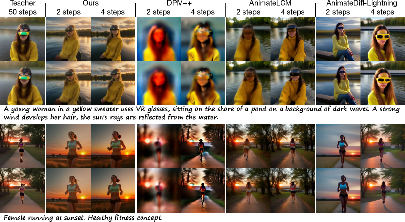
Figure 5: Qualitative comparison of video diffusion distillation with AnimateDiff [19] as the teacher model. The first and last frames are sampled for visualization. Our MCM produces cleaner frames using only 2 and 4 sampling steps, with better prompt alignment and improved frame details. Corresponding video results are in supplementary materials.

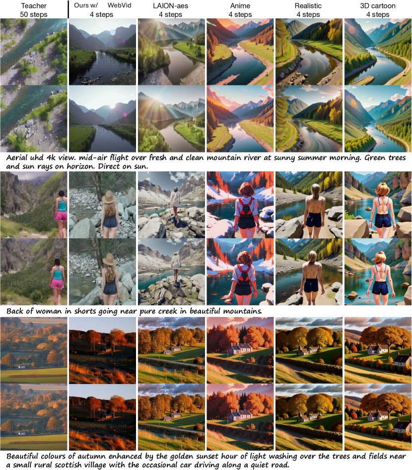
Figure 6: MCM frame quality improvement results using different image datasets with ModelScopeT2V [62] teacher. Our MCM effectively adapts to different distributions with 4 steps. Corresponding video results are in supplementary materials.

Table 3: Comparison on frame quality improvement. Performance is measured by FID using different numbers of sampling steps.

Method	FID $\downarrow$ (LAION-aes)				FID $\downarrow$ (Anime)
	1	2	4	8	1	2	4	8
Two-stage	110	119	115	122	160	159	149	150
MCM (ours)	82	69	73	76	78	71	67	69

Table 4: Ablation study on each components in MCM. ModelScopeT2V [62] is used as teacher.

Adv.	MCD	Mixed	FVD@Step $\downarrow$				CLIPSIM@Step $\uparrow$
			1	2	4	8	1	2	4	8
LCM [38]			854	658	603	637	27.50	29.28	30.48	30.73
$\checkmark$			703	650	767	760	28.70	30.37	30.90	30.77
$\checkmark$	$\checkmark$		563	526	548	579	29.30	30.40	30.11	29.52
$\checkmark$	$\checkmark$	$\checkmark$	526	450	456	503	29.81	30.63	30.55	29.58

Table 5: Ablation study on motion representation.

Motion	FVD@Step $\downarrow$				CLIPSIM@Step $\uparrow$
	1	2	4	8	1	2	4	8
Raw latent	703	650	767	760	28.70	30.37	30.90	30.77
Diff.	628	640	722	779	29.17	30.39	31.03	30.55
Corr.	659	699	727	725	28.83	30.39	30.62	30.62
Low freq.	677	667	753	919	29.25	30.32	30.35	29.79
High freq.	676	647	687	753	28.76	30.01	30.16	29.43
Learnable	563	526	548	579	29.30	30.40	30.11	29.52

Table 6: Ablation study on the mixed trajectory training.

$\lambda_{\text{real}}$	FVD@Step $\downarrow$				CLIPSIM@Step $\uparrow$
	1	2	4	8	1	2	4	8
1	563	526	548	579	29.30	30.40	30.11	29.52
0.5	526	450	456	503	29.81	30.63	30.55	29.58
0	556	498	483	523	28.77	29.73	29.93	29.53

4.1 Comparisons with distilled video diffusion models

Experiment settings. In this section, we compare MCM with other video diffusion models to validate the effectiveness of the disentangled motion-appearance distillation. For fair comparison, we use the WebVid 2M [5] as both the video and image training dataset, without using any additional image datasets. We postpone the experiments with different image datasets in Sec. 4.2. For testing, we randomly sample 500 validation videos from WebVid 2M (WebVid mini) for in-distribution evaluation; we also follow common practice [62, 16] to use $\sim$2900 validation videos from MSRVTT [70] for zero-shot generation evaluation. We report standard metrics of FVD and CLIPSIM.

Results. We compare our method with training-free samplers DDIM [54] and DPM++ [37], and trainable models LCM [38], AnimateLCM [61] and AnimateDiff-Lightning [35]. We present the quantitative results on WebVid and MSRVTT in Tab. 1 and Tab. 2, respectively. On both datasets, and using both teacher models AnimateDiff [19] and ModelScopeT2V [62], our MCM outperforms all competing distillation methods in terms of video quality and video-prompt alignment at sampling steps 1, 2, and 4. We compare the qualitative results in Fig. 5, where our method outputs clean video frames using 2 and 4 sampling steps. Compared with AnimateDiff-Lightning [35], we achieve better prompt-alignment and frame details, demonstrating our effectiveness.

4.2 Video distillation with improved frame quality

Experiment settings. In this section, we unleash the full capability of MCM by equipping the model with diverse types of image datasets. We showcase the effectiveness of using image datasets to boost frame quality as well as adapting the model to new styles without requiring corresponding video data. Specifically, we continue to use WebVid 2M [5] as the video dataset. For image dataset, we consider the following options. LAION-aes, a 4M subset sampled from the high-aesthetic image dataset LAION-Aesthetic 6+ [49]; datasets in anime, realistic, and 3D cartoon styles generated by fine-tuned StableDiffusion [3, 2, 1], each dataset containing 500k images with LAION captions.

Results. Due to the lack of prior arts with comparable capabilities, we validate by comparing MCM with a designed two-stage baseline. Following AnimateLCM [61], we implement a two-stage method: first training the spatial layers with the image dataset, then training the temporal layers with the video dataset. We use a real image dataset, LAION-aes, and a generated anime-style dataset for quantitative comparison. As shown in Tab. 4, our MCM achieves lower FID scores on both datasets, demonstrating its superior adaptability to different image dataset distributions. We present our qualitative results in Fig. 6, where our method demonstrates high frame quality using only four sampling steps, achieving sharp frames with various styles.

4.3 Ablation study

We conduct the distillation ablation study on WebVid mini [5] using ModelScopeT2V [62] as teacher. The main results are summarized in Tab. 4. Starting from LCM [38], we progressively add adversarial learning, motion consistency distillation loss, and mixed trajectory distillation. Each addition shows an improvement in video quality, demonstrating the effectiveness of these components.

Disentangled motion distribution. We compare different motion representations in Tab. 6. All representations, except for the latent low-frequency components, help reduce FVD and improve CLIPSIM at low sampling steps. This indicates that disentangling motion from the raw latent space for consistency learning enhances video quality. Among these, the learnable motion representation performs the best, demonstrating its effectiveness compared to handcrafted motion representations.

Mixed trajectory distribution. Tab. 6 compares the performance between using only real video ($\lambda_{\text{real}}=1$), only generated video ($\lambda_{\text{real}}=0$), or a mixed of both. The results reveal that mixing the trajectories achieves the best results. While using only generated videos also reduces FVD at all steps, it potentially leads to mode collapse, producing nearly all-black videos (Sec. B.1), highlighting the importance of incorporating real videos.

5 Conclusion

We introduce motion consistency model (MCM) to tackle the challenge of low frame quality in video diffusion distillation. Our method leverages disentangled motion distillation to separate motion learning from appearance learning, and mixed trajectory distillation to align training and inference through simulating the inference ODE trajectory. MCM achieves state-of-the-art video diffusion distillation results, and effectively improves frame quality when using a high-quality image dataset. Broader impacts and limitations. MCM accelerates and enhances video generation for creative applications. However, as a data-driven approach, our model is sensitive to the distribution and diversity of the training data, which influences model’s ability to generate varied video frames, potentially limiting generalization ability. MCM also carries potential risks such as deepfakes creation. Implementing responsible deployment is essential to mitigate these risks.

Appendix A Related work

Video generation. Early methods mainly rely on generative adversarial networks (GANs) [58, 6, 67, 53], which struggled with scalability and generalization to out-of-distribution domains. Building on the recent success of image diffusion models [22, 45], several methods leverage diffusion models for video generation [21, 24, 9, 62, 19, 65]. This paper focuses on two popular text-to-video diffusion models: ModelScopeT2V [62] and AnimateDiff [19]. ModelScopeT2V [62] inserts spatio-temporal blocks into 2D backbones and trains the whole backbone end-to-end, ensuring adaptability to varying frame lengths with smooth motions. AnimateDiff [19] introduces a plug-and-play motion module that learns motion priors from real-world videos and can be applied to personalized image diffusion models for video generation.

Diffusion distillation. Training-free methods primarily focus on developing advanced ODE solvers to reduce the number of sampling steps [54, 37, 7, 36, 73]. Another approach employs smaller backbones [39, 15, 32] to improve structural efficiency. To further reduce the inference steps, progressive distillation [46, 41, 34, 35] is first proposed to distill the two or more steps into one. Consistency models [55, 38, 66, 61] generalize progressive distillation by mapping any point on the PF-ODE trajectory to the same origin. A parallel line of work [71, 48, 34, 35, 31] directly applies constraints on the model output by leveraging adversarial losses. However, these methods heavily rely on the quality of the training dataset, and low-quality datasets inevitably degrade the generation quality.

Frame quality adjustment. Unlike image generation, which benefits from high-quality datasets [49], popular public video datasets [57, 70, 5] often exhibit lower frame quality, including issues like motion blur, low resolution, and watermarks. This discrepancy hinders the development of high-quality video generation in a single-stage, end-to-end manner. A straightforward way to improve frame quality is two-stage approach [9, 19, 61], which involves training an image backbone with a high-quality image dataset and then adding temporal layers for fine-tuning on video datasets Alternatively, some methods [29, 68] animate pre-trained image diffusion models with low-shot fine-tuning. In this paper, we propose a single-stage, end-to-end method to address this problem, while simultaneously achieving few-step sampling with video diffusion distillation.

Appendix B Additional experiments

B.1 Mixed trajectory distillation

We empirically find that only using generated videos for trajectory sampling (i.e., $\lambda_{\text{real}}=0$) may sometimes lead to near all-black videos, accounting for $\sim 5\%$ generated videos. Some examples are shown in Fig. 7. Such a result demonstrates the importance of leveraging real video data for the distillation.

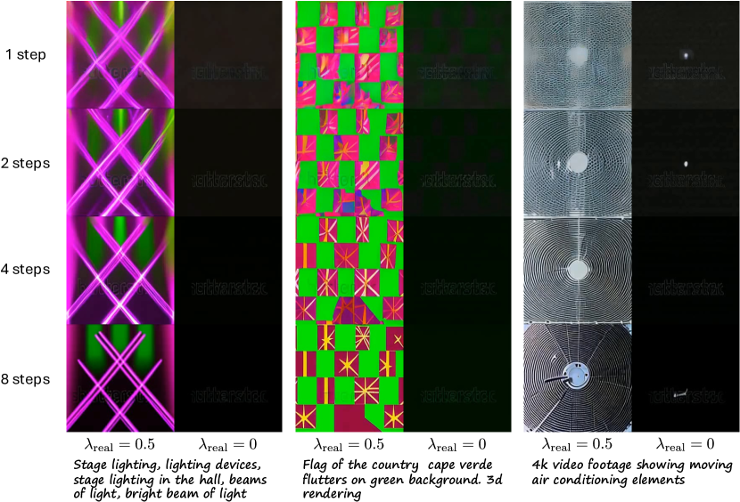
Figure 7: Failure case in mixed trajectory distillation when only generated videos are used for ODE trajectories sampling, i.e., $\lambda_{\text{real}}=0$.

Appendix C Additional implementation details

C.1 Image discriminator

We design our image discriminator based on StyleGAN-T [47] and ADD [48]. Specifically, given an input image, the discriminator first extracts features using a pre-trained, frozen DINOv2 [43, 14] model. Features are extracted from layers 2, 5, 8, and 11. These features are then passed through a set of trainable, lightweight discriminator heads to distinguish images at the patch level.

Following ADD [48], we use the ViT-S/14 variant for feature extraction. To improve video-caption alignment, we also incorporate CLIP embeddings for additional discriminator conditioning, following StyleGAN-T [47] and ADD [48]. For this, we use a CLIP-ViT-g-14 text encoder to compute text embeddings.

C.2 Training details

Both teachers use classifier-free guidance [23], and we follow LCM [38] to set a dynamic guidance scale range for distillation. Specifically, we set the guidance range values to $[5,15]$ for ModelScopeT2V [62], and $[7,8]$ for AnimateDiff [19]. We follow respective teachers to use $\epsilon$-prediction, and use linear beta scheduling for AnimateDiff following AnimateDiff-Lightning [35].

References

- [1] Disney pixar cartoon type b - v1.0. https://civitai.com/models/75650/disney-pixar-cartoon-type-b, 2023.
- [2] Realistic vision v6.0 b1. https://civitai.com/models/4201/realistic-vision-v60-b1, 2023.
- [3] Toonyou - beta 6. https://civitai.com/models/30240/toonyou, 2023.
- [4] Jason Ansel, Edward Yang, Horace He, Natalia Gimelshein, Animesh Jain, Michael Voznesensky, Bin Bao, Peter Bell, David Berard, Evgeni Burovski, et al. Pytorch 2: Faster machine learning through dynamic python bytecode transformation and graph compilation. In Proceedings of the 29th ACM International Conference on Architectural Support for Programming Languages and Operating Systems, Volume 2, pages 929–947, 2024.
- [5] Max Bain, Arsha Nagrani, Gül Varol, and Andrew Zisserman. Frozen in time: A joint video and image encoder for end-to-end retrieval. In Int. Conf. Comput. Vis., pages 1728–1738, 2021.
- [6] Yogesh Balaji, Martin Renqiang Min, Bing Bai, Rama Chellappa, and Hans Peter Graf. Conditional gan with discriminative filter generation for text-to-video synthesis. In IJCAI, volume 1, page 2, 2019.
- [7] Fan Bao, Chongxuan Li, Jun Zhu, and Bo Zhang. Analytic-dpm: an analytic estimate of the optimal reverse variance in diffusion probabilistic models. arXiv preprint arXiv:2201.06503, 2022.
- [8] James Betker, Gabriel Goh, Li Jing, Tim Brooks, Jianfeng Wang, Linjie Li, Long Ouyang, Juntang Zhuang, Joyce Lee, Yufei Guo, et al. Improving image generation with better captions. Computer Science. https://cdn. openai. com/papers/dall-e-3. pdf, 2(3):8, 2023.
- [9] Andreas Blattmann, Robin Rombach, Huan Ling, Tim Dockhorn, Seung Wook Kim, Sanja Fidler, and Karsten Kreis. Align your latents: High-resolution video synthesis with latent diffusion models. In IEEE Conf. Comput. Vis. Pattern Recog., pages 22563–22575, 2023.
- [10] Mathilde Caron, Hugo Touvron, Ishan Misra, Hervé Jégou, Julien Mairal, Piotr Bojanowski, and Armand Joulin. Emerging properties in self-supervised vision transformers. In Int. Conf. Comput. Vis., pages 9650–9660, 2021.
- [11] Ting Chen, Simon Kornblith, Mohammad Norouzi, and Geoffrey Hinton. A simple framework for contrastive learning of visual representations. pages 1597–1607. PMLR, 2020.
- [12] Xinlei Chen, Haoqi Fan, Ross Girshick, and Kaiming He. Improved baselines with momentum contrastive learning. arXiv preprint arXiv:2003.04297, 2020.
- [13] Xiaoliang Dai, Ji Hou, Chih-Yao Ma, Sam Tsai, Jialiang Wang, Rui Wang, Peizhao Zhang, Simon Vandenhende, Xiaofang Wang, Abhimanyu Dubey, et al. Emu: Enhancing image generation models using photogenic needles in a haystack. arXiv preprint arXiv:2309.15807, 2023.
- [14] Timothée Darcet, Maxime Oquab, Julien Mairal, and Piotr Bojanowski. Vision transformers need registers, 2023.
- [15] Gongfan Fang, Xinyin Ma, and Xinchao Wang. Structural pruning for diffusion models. Adv. Neural Inform. Process. Syst., 36, 2024.
- [16] Songwei Ge, Seungjun Nah, Guilin Liu, Tyler Poon, Andrew Tao, Bryan Catanzaro, David Jacobs, Jia-Bin Huang, Ming-Yu Liu, and Yogesh Balaji. Preserve your own correlation: A noise prior for video diffusion models. In Int. Conf. Comput. Vis., pages 22930–22941, 2023.
- [17] Jean-Bastien Grill, Florian Strub, Florent Altché, Corentin Tallec, Pierre Richemond, Elena Buchatskaya, Carl Doersch, Bernardo Avila Pires, Zhaohan Guo, Mohammad Gheshlaghi Azar, et al. Bootstrap your own latent-a new approach to self-supervised learning. Adv. Neural Inform. Process. Syst., 33:21271–21284, 2020.
- [18] Ishaan Gulrajani, Faruk Ahmed, Martin Arjovsky, Vincent Dumoulin, and Aaron C Courville. Improved training of wasserstein gans. Adv. Neural Inform. Process. Syst., 30, 2017.
- [19] Yuwei Guo, Ceyuan Yang, Anyi Rao, Yaohui Wang, Yu Qiao, Dahua Lin, and Bo Dai. Animatediff: Animate your personalized text-to-image diffusion models without specific tuning. arXiv preprint arXiv:2307.04725, 2023.
- [20] Martin Heusel, Hubert Ramsauer, Thomas Unterthiner, Bernhard Nessler, and Sepp Hochreiter. Gans trained by a two time-scale update rule converge to a local nash equilibrium. Adv. Neural Inform. Process. Syst., 30, 2017.
- [21] Jonathan Ho, William Chan, Chitwan Saharia, Jay Whang, Ruiqi Gao, Alexey Gritsenko, Diederik P Kingma, Ben Poole, Mohammad Norouzi, David J Fleet, et al. Imagen video: High definition video generation with diffusion models. arXiv preprint arXiv:2210.02303, 2022.
- [22] Jonathan Ho, Ajay Jain, and Pieter Abbeel. Denoising diffusion probabilistic models. Adv. Neural Inform. Process. Syst., 33:6840–6851, 2020.
- [23] Jonathan Ho and Tim Salimans. Classifier-free diffusion guidance. arXiv preprint arXiv:2207.12598, 2022.
- [24] Jonathan Ho, Tim Salimans, Alexey Gritsenko, William Chan, Mohammad Norouzi, and David J Fleet. Video diffusion models. Adv. Neural Inform. Process. Syst., 35:8633–8646, 2022.
- [25] Edward J Hu, Yelong Shen, Phillip Wallis, Zeyuan Allen-Zhu, Yuanzhi Li, Shean Wang, Lu Wang, and Weizhu Chen. Lora: Low-rank adaptation of large language models. arXiv preprint arXiv:2106.09685, 2021.
- [26] Zhaoyang Huang, Xiaoyu Shi, Chao Zhang, Qiang Wang, Ka Chun Cheung, Hongwei Qin, Jifeng Dai, and Hongsheng Li. Flowformer: A transformer architecture for optical flow. In Eur. Conf. Comput. Vis., pages 668–685. Springer, 2022.
- [27] Phillip Isola, Jun-Yan Zhu, Tinghui Zhou, and Alexei A Efros. Image-to-image translation with conditional adversarial networks. In IEEE Conf. Comput. Vis. Pattern Recog., pages 1125–1134, 2017.
- [28] Tero Karras, Miika Aittala, Timo Aila, and Samuli Laine. Elucidating the design space of diffusion-based generative models. Adv. Neural Inform. Process. Syst., 35:26565–26577, 2022.
- [29] Levon Khachatryan, Andranik Movsisyan, Vahram Tadevosyan, Roberto Henschel, Zhangyang Wang, Shant Navasardyan, and Humphrey Shi. Text2video-zero: Text-to-image diffusion models are zero-shot video generators. In Int. Conf. Comput. Vis., pages 15954–15964, 2023.
- [30] Diederik P Kingma and Jimmy Ba. Adam: A method for stochastic optimization. arXiv preprint arXiv:1412.6980, 2014.
- [31] Jonas Kohler, Albert Pumarola, Edgar Schönfeld, Artsiom Sanakoyeu, Roshan Sumbaly, Peter Vajda, and Ali Thabet. Imagine flash: Accelerating emu diffusion models with backward distillation. arXiv preprint arXiv:2405.05224, 2024.
- [32] Yanyu Li, Huan Wang, Qing Jin, Ju Hu, Pavlo Chemerys, Yun Fu, Yanzhi Wang, Sergey Tulyakov, and Jian Ren. Snapfusion: Text-to-image diffusion model on mobile devices within two seconds. Adv. Neural Inform. Process. Syst., 36, 2024.
- [33] Shanchuan Lin, Bingchen Liu, Jiashi Li, and Xiao Yang. Common diffusion noise schedules and sample steps are flawed. In IEEE Winter Conf. Appl. Comput. Vis., pages 5404–5411, 2024.
- [34] Shanchuan Lin, Anran Wang, and Xiao Yang. Sdxl-lightning: Progressive adversarial diffusion distillation. arXiv preprint arXiv:2402.13929, 2024.
- [35] Shanchuan Lin and Xiao Yang. Animatediff-lightning: Cross-model diffusion distillation. arXiv preprint arXiv:2403.12706, 2024.
- [36] Luping Liu, Yi Ren, Zhijie Lin, and Zhou Zhao. Pseudo numerical methods for diffusion models on manifolds. arXiv preprint arXiv:2202.09778, 2022.
- [37] Cheng Lu, Yuhao Zhou, Fan Bao, Jianfei Chen, Chongxuan Li, and Jun Zhu. Dpm-solver: A fast ode solver for diffusion probabilistic model sampling in around 10 steps. Adv. Neural Inform. Process. Syst., 35:5775–5787, 2022.
- [38] Simian Luo, Yiqin Tan, Longbo Huang, Jian Li, and Hang Zhao. Latent consistency models: Synthesizing high-resolution images with few-step inference. arXiv preprint arXiv:2310.04378, 2023.
- [39] Xinyin Ma, Gongfan Fang, and Xinchao Wang. Deepcache: Accelerating diffusion models for free. arXiv preprint arXiv:2312.00858, 2023.
- [40] Sourab Mangrulkar, Sylvain Gugger, Lysandre Debut, Younes Belkada, Sayak Paul, and Benjamin Bossan. Peft: State-of-the-art parameter-efficient fine-tuning methods. https://github.com/huggingface/peft, 2022.
- [41] Chenlin Meng, Robin Rombach, Ruiqi Gao, Diederik Kingma, Stefano Ermon, Jonathan Ho, and Tim Salimans. On distillation of guided diffusion models. In IEEE Conf. Comput. Vis. Pattern Recog., pages 14297–14306, 2023.
- [42] Alexander Quinn Nichol and Prafulla Dhariwal. Improved denoising diffusion probabilistic models. pages 8162–8171. PMLR, 2021.
- [43] Maxime Oquab, Timothée Darcet, Theo Moutakanni, Huy V. Vo, Marc Szafraniec, Vasil Khalidov, Pierre Fernandez, Daniel Haziza, Francisco Massa, Alaaeldin El-Nouby, Russell Howes, Po-Yao Huang, Hu Xu, Vasu Sharma, Shang-Wen Li, Wojciech Galuba, Mike Rabbat, Mido Assran, Nicolas Ballas, Gabriel Synnaeve, Ishan Misra, Herve Jegou, Julien Mairal, Patrick Labatut, Armand Joulin, and Piotr Bojanowski. Dinov2: Learning robust visual features without supervision, 2023.
- [44] Alec Radford, Jong Wook Kim, Chris Hallacy, Aditya Ramesh, Gabriel Goh, Sandhini Agarwal, Girish Sastry, Amanda Askell, Pamela Mishkin, Jack Clark, et al. Learning transferable visual models from natural language supervision. pages 8748–8763. PMLR, 2021.
- [45] Robin Rombach, Andreas Blattmann, Dominik Lorenz, Patrick Esser, and Björn Ommer. High-resolution image synthesis with latent diffusion models. In IEEE Conf. Comput. Vis. Pattern Recog., pages 10684–10695, 2022.
- [46] Tim Salimans and Jonathan Ho. Progressive distillation for fast sampling of diffusion models. arXiv preprint arXiv:2202.00512, 2022.
- [47] Axel Sauer, Tero Karras, Samuli Laine, Andreas Geiger, and Timo Aila. Stylegan-t: Unlocking the power of gans for fast large-scale text-to-image synthesis. pages 30105–30118. PMLR, 2023.
- [48] Axel Sauer, Dominik Lorenz, Andreas Blattmann, and Robin Rombach. Adversarial diffusion distillation. arXiv preprint arXiv:2311.17042, 2023.
- [49] Christoph Schuhmann, Romain Beaumont, Richard Vencu, Cade Gordon, Ross Wightman, Mehdi Cherti, Theo Coombes, Aarush Katta, Clayton Mullis, Mitchell Wortsman, et al. Laion-5b: An open large-scale dataset for training next generation image-text models. Adv. Neural Inform. Process. Syst., 35:25278–25294, 2022.
- [50] Xiaoyu Shi, Zhaoyang Huang, Weikang Bian, Dasong Li, Manyuan Zhang, Ka Chun Cheung, Simon See, Hongwei Qin, Jifeng Dai, and Hongsheng Li. Videoflow: Exploiting temporal cues for multi-frame optical flow estimation. In Int. Conf. Comput. Vis., pages 12469–12480, 2023.
- [51] Xiaoyu Shi, Zhaoyang Huang, Dasong Li, Manyuan Zhang, Ka Chun Cheung, Simon See, Hongwei Qin, Jifeng Dai, and Hongsheng Li. Flowformer++: Masked cost volume autoencoding for pretraining optical flow estimation. In IEEE Conf. Comput. Vis. Pattern Recog., pages 1599–1610, 2023.
- [52] Karen Simonyan and Andrew Zisserman. Two-stream convolutional networks for action recognition in videos. Adv. Neural Inform. Process. Syst., 27, 2014.
- [53] Ivan Skorokhodov, Sergey Tulyakov, and Mohamed Elhoseiny. Stylegan-v: A continuous video generator with the price, image quality and perks of stylegan2. In IEEE Conf. Comput. Vis. Pattern Recog., pages 3626–3636, 2022.
- [54] Jiaming Song, Chenlin Meng, and Stefano Ermon. Denoising diffusion implicit models. arXiv preprint arXiv:2010.02502, 2020.
- [55] Yang Song, Prafulla Dhariwal, Mark Chen, and Ilya Sutskever. Consistency models. arXiv preprint arXiv:2303.01469, 2023.
- [56] Yang Song, Jascha Sohl-Dickstein, Diederik P Kingma, Abhishek Kumar, Stefano Ermon, and Ben Poole. Score-based generative modeling through stochastic differential equations. arXiv preprint arXiv:2011.13456, 2020.
- [57] Khurram Soomro, Amir Roshan Zamir, and Mubarak Shah. Ucf101: A dataset of 101 human actions classes from videos in the wild. arXiv preprint arXiv:1212.0402, 2012.
- [58] Sergey Tulyakov, Ming-Yu Liu, Xiaodong Yang, and Jan Kautz. Mocogan: Decomposing motion and content for video generation. In IEEE Conf. Comput. Vis. Pattern Recog., pages 1526–1535, 2018.
- [59] Thomas Unterthiner, Sjoerd Van Steenkiste, Karol Kurach, Raphael Marinier, Marcin Michalski, and Sylvain Gelly. Towards accurate generative models of video: A new metric & challenges. arXiv preprint arXiv:1812.01717, 2018.
- [60] Patrick von Platen, Suraj Patil, Anton Lozhkov, Pedro Cuenca, Nathan Lambert, Kashif Rasul, Mishig Davaadorj, Dhruv Nair, Sayak Paul, William Berman, Yiyi Xu, Steven Liu, and Thomas Wolf. Diffusers: State-of-the-art diffusion models. https://github.com/huggingface/diffusers, 2022.
- [61] Fu-Yun Wang, Zhaoyang Huang, Xiaoyu Shi, Weikang Bian, Guanglu Song, Yu Liu, and Hongsheng Li. Animatelcm: Accelerating the animation of personalized diffusion models and adapters with decoupled consistency learning. arXiv preprint arXiv:2402.00769, 2024.
- [62] Jiuniu Wang, Hangjie Yuan, Dayou Chen, Yingya Zhang, Xiang Wang, and Shiwei Zhang. Modelscope text-to-video technical report. arXiv preprint arXiv:2308.06571, 2023.
- [63] Limin Wang, Yuanjun Xiong, Dahua Lin, and Luc Van Gool. Untrimmednets for weakly supervised action recognition and detection. In IEEE Conf. Comput. Vis. Pattern Recog., pages 4325–4334, 2017.
- [64] Limin Wang, Yuanjun Xiong, Zhe Wang, Yu Qiao, Dahua Lin, Xiaoou Tang, and Luc Van Gool. Temporal segment networks: Towards good practices for deep action recognition. In Eur. Conf. Comput. Vis., pages 20–36. Springer, 2016.
- [65] Xiang Wang, Hangjie Yuan, Shiwei Zhang, Dayou Chen, Jiuniu Wang, Yingya Zhang, Yujun Shen, Deli Zhao, and Jingren Zhou. Videocomposer: Compositional video synthesis with motion controllability. Adv. Neural Inform. Process. Syst., 36, 2024.
- [66] Xiang Wang, Shiwei Zhang, Han Zhang, Yu Liu, Yingya Zhang, Changxin Gao, and Nong Sang. Videolcm: Video latent consistency model. arXiv preprint arXiv:2312.09109, 2023.
- [67] Yaohui Wang, Piotr Bilinski, Francois Bremond, and Antitza Dantcheva. G3an: Disentangling appearance and motion for video generation. In IEEE Conf. Comput. Vis. Pattern Recog., pages 5264–5273, 2020.
- [68] Jay Zhangjie Wu, Yixiao Ge, Xintao Wang, Stan Weixian Lei, Yuchao Gu, Yufei Shi, Wynne Hsu, Ying Shan, Xiaohu Qie, and Mike Zheng Shou. Tune-a-video: One-shot tuning of image diffusion models for text-to-video generation. In Int. Conf. Comput. Vis., pages 7623–7633, 2023.
- [69] Tianxing Wu, Chenyang Si, Yuming Jiang, Ziqi Huang, and Ziwei Liu. Freeinit: Bridging initialization gap in video diffusion models. arXiv preprint arXiv:2312.07537, 2023.
- [70] Jun Xu, Tao Mei, Ting Yao, and Yong Rui. Msr-vtt: A large video description dataset for bridging video and language. In IEEE Conf. Comput. Vis. Pattern Recog., pages 5288–5296, 2016.
- [71] Yanwu Xu, Yang Zhao, Zhisheng Xiao, and Tingbo Hou. Ufogen: You forward once large scale text-to-image generation via diffusion gans. arXiv preprint arXiv:2311.09257, 2023.
- [72] Hangjie Yuan, Shiwei Zhang, Xiang Wang, Yujie Wei, Tao Feng, Yining Pan, Yingya Zhang, Ziwei Liu, Samuel Albanie, and Dong Ni. Instructvideo: Instructing video diffusion models with human feedback. arXiv preprint arXiv:2312.12490, 2023.
- [73] Qinsheng Zhang and Yongxin Chen. Fast sampling of diffusion models with exponential integrator. arXiv preprint arXiv:2204.13902, 2022.
- [74] Yue Zhao, Yuanjun Xiong, and Dahua Lin. Recognize actions by disentangling components of dynamics. In IEEE Conf. Comput. Vis. Pattern Recog., pages 6566–6575, 2018.
- [75] Jun-Yan Zhu, Taesung Park, Phillip Isola, and Alexei A Efros. Unpaired image-to-image translation using cycle-consistent adversarial networks. In Int. Conf. Comput. Vis., pages 2223–2232, 2017.