Causality for Complex Continuous-time Functional Longitudinal Studies with Dynamic Treatment Regimes
Abstract
Causal inference in longitudinal studies is often hampered by treatment-confounder feedback. Existing methods typically assume discrete time steps or step-like data changes, which we term “regular and irregular functional studies,” limiting their applicability to studies with continuous monitoring data, like intensive care units or continuous glucose monitoring. These studies, which we formally term “functional longitudinal studies,” require new approaches. Moreover, existing methods tailored for “functional longitudinal studies” can only investigate static treatment regimes, which are independent of historical covariates or treatments, leading to either stringent parametric assumptions or strong positivity assumptions. This restriction has limited the range of causal questions these methods can answer and their practicality. We address these limitations by developing a nonparametric framework for functional longitudinal data, accommodating dynamic treatment regimes that depend on historical covariates or treatments, and may or may not depend on the actual treatment administered. To build intuition and explain our approach, we provide a comprehensive review of existing methods for regular and irregular longitudinal studies. We then formally define the potential outcomes and causal effects of interest, develop identification assumptions, and derive g-computation and inverse probability weighting formulas through novel applications of stochastic process and measure theory. Additionally, we compute the efficient influence curve using semiparametric theory. Our framework generalizes existing literature, and achieves double robustness under specific conditions. Finally, to aid interpretation, we provide sufficient and intuitive conditions for our identification assumptions, enhancing the applicability of our methodology to real-world scenarios.
keywords:
[class=MSC]keywords:
1 Introduction
1.1 Background
Establishing causality is a fundamental goal in scientific research, particularly in fields such as medicine and social sciences. While randomized controlled trials are considered the gold standard for causal inference, they may not always be feasible or ethical. Observational studies, especially those involving complex longitudinal data, pose unique challenges for causal inference due to the presence of time-varying confounders and the need to account for the dynamic nature of treatment and outcome processes.
Functional longitudinal data, characterized by continuous-time processes and high-dimensional measurements, present additional complexities for causal inference. The presence of an infinite number of potential treatment-confounder feedback loops and the lack of a joint density for these processes require novel methodological approaches. Existing methods developed for regular and irregular longitudinal data may not be directly applicable to functional longitudinal data, necessitating the development of a rigorous theoretical framework tailored to this setting.
Traditional methods of adjustment, such as regression models that incorporate a history of treatments and confounders, often fall short in these scenarios. These methods typically assume that confounders are static and do not take into account the dynamic feedback loop between treatment and confounding variables over time. Intervening on past treatment values, a critical aspect in such studies, necessitates accounting for changes in future confounders. These future confounders must then be carefully conditioned upon to correct for confounding. This creates a complex interplay of variables across different time points, complicating the process of establishing clear causal links.
Given these challenges, there is a pressing need for more sophisticated and nuanced methods of causal inference that can effectively handle the intricacies of longitudinal data. Developing these methods is not just an academic exercise; it has profound implications for how we understand and intervene in a range of fields, from healthcare to social policy. As such, the pursuit of advancing causal inference techniques in the context of complex longitudinal studies is both a formidable challenge and an imperative for continued progress in scientific research. In light of these challenges, this paper aims to develop a comprehensive theoretical framework for causal inference in functional longitudinal data under all dynamic treatment regimes, filling an important gap in the current literature.
1.1.1 Longitudinal data formats
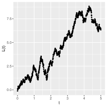
To gain a deeper insight into the complexities of functional longitudinal data, it is crucial to first examine the various formats of longitudinal data and their unique features. These datasets can be classified into three primary types. The first type, ”Regular Longitudinal Data (RLD),” involves data collected at set, regular intervals, though this may not accurately reflect the unpredictable nature of visit timings. The second type, ”Irregular Longitudinal Data (ILD),” consists of data where changes in treatment and confounders occur in discrete, finite steps, resembling point processes. This type is common in pharmacoeconomic studies, where patient visits and treatment adjustments happen randomly but within finite periods. The third type, ”Functional Longitudinal Data (FLD),” has emerged with advancements in real-time monitoring technologies in healthcare, characterized by continuous tracking of confounders and treatments. This type of data is common in intensive care and chronic disease management using wearable devices, which results in numerous feedback loops between treatment and confounders, thereby complicating causal inference due to the absence of a joint density for these variables. Figures 1 and 2 provide a visual representation of the distinct characteristics and relationships of these data types.


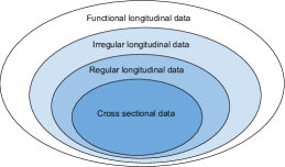
It is evident and important to realize that both RLD and ILD are special cases of FLD, as shown in the left figure of Figure 2. Therefore, methods designed for FLD can be applied to RLD and ILD, but typically not vice versa. Existing frameworks tailored for RLD or ILD cannot be straightforwardly applied to FLD. Intentional or unintentional usage of existing frameworks on FLD, for instance, pruning FLD into RLD, is prone to errors and hence might lead to unwanted causal conclusions, which can have serious vital consequences and result in a waste of healthcare resources. See Ying (2022, 2024) for a detailed discussion of the distinctions between the three types of longitudinal data.
1.1.2 Treatment regimes
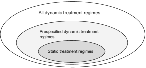
In addition to the complexity introduced by functional longitudinal data, the presence of time-varying treatments and the need to consider dynamic treatment regimes further complicate causal inference in this setting. A Treatment Regime (TR), also referred to as a strategy, plan, policy, or protocol, is a rule to assign treatment at each time of follow-up (Hernán and Robins, 2020). It is called a Static TR (STR) if it only depends on past treatment, while it is called a Dynamic TR (DTR) if it further depends on past covariates and outcomes. It is called deterministic if it is a determined function of past information, while it is called stochastic or random if it is random. For example, in a cross-sectional study, the average treatment effect focuses on a contrast between the averages of counterfactual outcomes if treatment were to be set to everyone or no one. This is static because it does not depend on covariates and deterministic because it is fixed. Suppose we define a rule that any patient were to receive treatment with 50% chance, then this is a stochastic STR. If, over age 65 were not to be treated while under age 65 were to be treated, then this is a deterministic DTR. If the patient under age 65 has a 50% chance of being treated, then this is a stochastic DTR. Apparently, deterministic TRs and STRs are special cases of stochastic TRs and DTRs, respectively.
It is important to note that previous literature almost exclusively investigates prespecified DTRs, that is, DTRs that are known and independent of the actual TR, though in most cases they have abused the name DTR. Recent works have started to consider DTRs that depend on the actual TRs. For example, Haneuse and Rotnitzky (2013) considered “modified treatment policy” to answer what happens if, say, some continuous treatment dosage were to be added by some values. Robins, Hernán and SiEBERT (2004); Taubman et al. (2009) considered the “threshold intervention” to answer what happens if some continuous treatment like physical activity were to be set to a threshold if below but otherwise kept unchanged. Kennedy (2019) considered the so-called “incremental interventions” to shift the odds of receiving treatment and answered what happens if everyone’s odds of receiving treatment were, for instance, doubled compared to the actual odds. Young, Hernán and Robins (2014); Díaz and van der Laan (2012) both considered DTRs depending on actual TRs, where Díaz and van der Laan (2012) focused on “shift interventions”, for example, the effect of a policy that encourages people to exercise more, leading to a population where the distribution of physical activity is shifted according to certain health and socioeconomic variables. Therefore, distinguishing treatment regimes is not only a mathematical consideration but, more importantly, about what causal questions one is raising. In this paper, we investigate all DTRs (ADTRs), that is, we allow DTRs to depend on either the actual TR or not.
1.2 Objectives and Contributions
Functional longitudinal data (FLD) presents unique challenges for causal inference that are not adequately addressed by existing methods developed for regular or irregular longitudinal data. The continuous-time nature of FLD, coupled with the presence of an infinite number of potential treatment-confounder feedback loops, requires a novel theoretical framework that can account for these complexities. Existing methods often rely on the presence of a joint density for the treatment and confounder processes, which is not available in the FLD setting, and may make simplifying assumptions that do not hold for FLD. Furthermore, most existing methods for FLD focus on STRs, which may not be realistic in many real-world settings.
The primary objective of this paper is to develop a rigorous theoretical framework for causal inference in FLD under ADTRs. This framework aims to address the limitations of existing methods and provide a foundation for the development of practical estimation methods and algorithms. Our goal is not only to integrate and build upon the existing literature but also to extend the boundaries of our understanding by developing a corresponding semiparametric theory. Note that both the longitudinal data (FLD) and the treatment regimes (ADTRs) are as general as they can be (weakest to none assumptions on their formats).
To develop our framework, we draw inspiration from the concept of the Riemann integral. In the context of integration, one cannot simply evaluate the function point by point, as there are uncountably infinite points along the real number line. The Riemann integral bridges this gap between the finite and the infinite by partitioning the domain into smaller intervals and considering the function’s behavior within each interval. As the number of intervals increases and their width tends to zero, the Riemann sum converges to the true integral value.
Similarly, in the context of causal inference for FLD, we face the challenge of dealing with an uncountably infinite number of treatment-confounder feedback loops. Attempting to handle each time point individually, as one might do in the case of regular longitudinal data (RLD), becomes intractable. Moreover, without considering one point at a time, we lose access to a well-defined density function, which creates a tension between the existing theory based on densities and the theory needed for FLD.
Guided by this intuition, our key contributions are as follows:
-
1.
We generalize the potential outcome framework for FLD under ADTR, which is surprisingly a nontrivial task.
-
2.
We propose a novel set of assumptions tailored to the FLD setting, enabling the identification of causal effects under ADTRs. We construct a comprehensive identification framework for causal inference in FLD under ADTRs, including the development of g-computation, inverse probability weighting (IPW), and doubly robust formulas.
-
3.
We develop the semiparametric theory, including the derivation of the efficient influence curve (EIC), providing a basis for optimal estimators and inference procedures in the future.
-
4.
We discuss the implications of our results for practice and provide guidance on interpreting our key assumptions in real-world settings. We demonstrate the generality of our framework by showing how it subsumes existing methods for regular and irregular longitudinal data as special cases.
By addressing these objectives and making these contributions, we aim to fill an important gap in the current literature on causal inference for complex longitudinal data. Our theoretical framework provides a foundation for the development of practical estimation methods and algorithms, paving the way for more effective treatment strategies in various domains, such as healthcare and social policy.
The identification framework and semiparametric theory can be directly applied to:
-
1.
RLD with functional data observation at each regular observed time point ;
-
2.
ILD with functional data observation at each jumping time ;
-
3.
Studies on continuous time to treatment switching, initialization, or termination where timing is of interest;
-
4.
ILD where incremental intervention, threshold intervention, or increasing intervention might be of interest;
-
5.
Semi-Functional Longitudinal Data (SFLD) which we define as a data type standing between ILD and FLD, where the treatment process is ILD and the covariate process is allowed to be FLD.
The remainder of this paper is organized as follows: Section 2 provides a review of existing methods for causal inference in regular and irregular longitudinal data, highlighting their limitations when applied to FLD. Therein we also review Ying (2022). Section 3 introduces the concept of ”all dynamic treatment regimes” (ADTR) and provides a rigorous mathematical definition of the causal quantity of interest in the FLD setting. Section 4 presents our causal identification framework for FLD under ADTR, including the key assumptions and the derivation of the g-computation and inverse probability weighting (IPW) formulas. In this Section we also discuss the recursive representations of the g-computation and IPW processes, presents the doubly robust formula. Section 5 develops the semiparametric theory for our proposed estimators, deriving the efficient influence function (EIF) and discussing its implications. Section 6 provides guidance on interpreting our key assumptions and results in practice. Finally, Section 7 concludes the paper with a summary of our main contributions and a discussion of future research directions. Proofs of our results are given in the appendix.
1.3 Preliminaries
Throughout the rest of the paper, suppose that there is a longitudinal study during 0 to .
-
1.
Define as the underlying sample space and -algebra. Write as the probability measure, where is the set of all probability measures on .
-
2.
are treatments received at time , which can be multi-dimensional binary, categorical or continuous measurable random mapping defined on . We write and abbreviate . We define as the set of all possible values of .
-
3.
are measured confounders at time , which can be multi-dimensional binary, categorical, or continuous measurable random mapping defined on . We write and abbreviate . For convenience, we write , a subset of , as the outcomes of interest. We include the outcomes into covariates to reflect the fact that both past outcomes and covariates influence current treatment, which can affect both future outcomes and covariates.
-
4.
Note that and measured at a single time in principle can be functional data themselves with measure theory we will leverage. However, such consideration has been rarely considered for cross sectional studies (Miao, Xue and Zhang, 2020; Zhang et al., 2021; Tan et al., 2022) and not yet for regular or irregular longitudinal studies. Therefore, for easier reviews later in Section 2, we assume they are multi-dimensional binary, categorical, or continuous, at least for Section 2.
-
5.
Also, write the counterfactual covariates and counterfactual outcomes , for any , as the covariates and outcomes if the treatment were to set as . These counterfactuals are considered to be defined pre-treatment. Note that counterfactual covariates and outcomes under DTRs are functions of and . There is individual subtlety when defining them and therefore we will define them one by one for RLD, ILD, and FLD later. In principle, we could define counterfactual censoring time as well but we drop this because we do not care the causal effect on censoring time. We write and .
-
6.
When there is no confusion, we may write to represent the distribution on the path space induced by the stochastic processes and the probability measure on the sample space . Note that this is not a density. This notation is well adopted by probabilists (Bhattacharya and Waymire, 2007; Durrett, 2019) and also statisticians (Gill and Robins, 2001).
-
7.
We assume the event space is Polish so that conditional probability can be chosen to be regular. We understand conditional distribution as a function over a sigma algebra multiplied with a path set. For instance, can be seen as a function over Borel space generated by and the path set . Importantly, conditional distribution is defined almost surely and one needs to take extra caution when replacing and intervening treatment distributions when conducting causal inference.
-
8.
For any two probability distribution and on , and two temporary random variables , we write as the Radon-Nikodym derivative. It is understood as a function of such that for any measurable function , .
-
9.
We use the upper case for random variables and the lower case for their realized values. An important caveat is that conditional probability is only uniquely defined almost surely. Therefore throughout this draft, otherwise stated, for the measure zero subset where the conditional probability is not uniquely defined, we set the conditional probability to be zero.
-
10.
Starting from Section 3, we define additional notation for mortality and censoring, filtration, partition and total variation norm:
-
•
To accommodate mortality and censoring in our framework, we consider as a time-to-event endpoint, for instance, death, and as the right censoring time, both of which are terminating states. Define as the censored event time. To ease notation, we include into and set whenever .
-
•
Note that and are not observed for or defined for . We can offset and for observed data whenever and and for censoring free data whenever . Therefore, and is always well defined and observed for any . Also, the information of is absorbed into and .
-
•
Thus the observed data are and the uncensored full data are .
-
•
Define as the natural filtration and . We also define as a one-step treatment aware filtration. Note that is a stopping time of and , thus we may write and . We manually write and as the trivial sigma algebra for convenience.
-
•
A partition on is a finite sequence of numbers of the form . The mesh of a partition is , representing the maximum gap length of the partition.
-
•
We use to represent the total variation norm over the space of signed measures of the path space, which is a Banach space.
-
•
-
11.
Starting from Section 5, we define Gâteaux derivative. For any two probability distribution and on , we write as the Gâteaux derivative of to the direction by , understood in the linear space of all signed measure on .
These following examples were previously introduced in Ying (2022), and are expanded upon here in the context of the generalized framework.
Example 1 (Intensive care unit).
The widespread adoption of electronic health records (EHRs) has resulted in an extensive collection of clinical data across hospitals in the United States. The Intensive Care Unit (ICU) is a particularly rich source of data due to the continuous monitoring and critical interventions provided to patients. This environment demands a sophisticated data infrastructure to accurately capture the temporal details of patient care. The Medical Information Mart for Intensive Care IV (MIMIC-IV) (Johnson et al., 2023), an openly available EHR database, addresses this need by offering detailed, time-stamped data on ICU patients. MIMIC-IV goes beyond static health records by providing functional longitudinal data (FLD), which includes continuous streams of physiological measurements, lab results, medication records, and clinical events. This detailed dataset enables researchers to move past simple correlations and investigate the dynamic interactions affecting patient outcomes. Key factors such as treatment timing and duration are crucial for understanding the effectiveness of interventions. For example, could represent the administration of antibiotics at time , while might encompass variables such as illness severity scores, vital signs, lab results, urine output, and other relevant patient data. Researchers can specify treatment regimes to study the impact of antibiotic use on patient recovery in the ICU.
Example 2 (Continuous glucose monitoring).
Continuous glucose monitoring (CGM) Continuous glucose monitoring (CGM) (Klonoff, 2005; Rodbard, 2016; Klonoff, Ahn and Drincic, 2017) has become an increasingly popular tool for patients requiring insulin, offering detailed insights into glycemic variations that are not possible with intermittent capillary blood glucose measurements. CGM aids patients in managing diabetes through real-time data, enabling timely lifestyle and medication adjustments. The introduction of CGM has revolutionized the understanding of glycemia by providing continuous, high-resolution data streams that capture glucose fluctuations in interstitial fluid every few minutes. This transforms CGM data into functional longitudinal data (FLD), requiring a new statistical approach that considers temporal dependencies and physiological variations over time. Unlike static blood glucose measurements, CGM data present a dynamic and intricate picture of glycemic control. For instance, might represent insulin administration at time , while could include glucose levels and immediate changes due to diet, medication, or physical activity at time . Researchers can design specific treatment regimes to explore the impact of various insulin dosages, frequencies, and timings on glucose levels.
2 A Review for Longitudinal Studies
In this section, we give more thorough reviews on causal definitions and identification procedures in regular longitudinal studies in Section 2.1 and irregular longitudinal studies in Section 2.2. We summarize their assumptions (assumptions on paths of the underlying stochastic processes) and distributional assumptions (assumptions on the underlying distribution). We skip literature about STRs for RLD and ILD. For interested readers, see Ying (2022, 2024). We mainly borrow results from the literature mentioned earlier, however, we adjust them to our settings and add our understanding along the way, which can motivate our framework as well. Finally, we review Ying (2022, 2024) in Section 2.3. We ignore time-to-event variable and censoring in this section to sharp the focus and ground ideas.
See Table 1 for a summary of literature review. Apparently from the table, there are research gaps in several directions. There is no consideration of causal inference under PDTRs for FLD. There is rarely any investigation of more general ADTR considered, very recently for RLD, nothing for ILD, let alone FLD.
| Model-based methods | |||
|---|---|---|---|
| RLD |
|
||
| ILD |
|
||
| FLD | Singer (2008); Commenges and Gégout-Petit (2009); Sun and Crawford (2022) | ||
| Estimand-based methods for STRs | |||
| RLD |
|
||
| ILD | Rytgaard, Gerds and van der Laan (2022) | ||
| FLD | Ying (2022, 2024) | ||
| Estimand-based methods for PDTRs | |||
| RLD |
|
||
| ILD | Rytgaard, Gerds and van der Laan (2022) | ||
| FLD | This paper | ||
| Estimand-based methods for ADTRs | |||
| RLD |
|
||
| ILD | This paper | ||
| FLD | This paper | ||
2.1 Regular longitudinal studies
Suppose the aforementioned longitudinal study is a regular longitudinal study conducted on fixed time . To connect with our notation, we may set . Obviously, and (hence ) may only change at and , and . The event time and censoring time may only take values in . For a finite number of random variables, the measure on the path space induced by gives rise to a multivariate distribution function. We use as the observed data density or probability mass function. Likewise, we use to denote conditional density or condition probability mass function.
The observed data likelihood admits a unique Markov’s factorization according to the temporal order as
| (1) |
where as convenience. Therefore, the observed TR is for any . Consider an ADTR , where the subscript means may depend on the observed TR, the counterfactual outcome under is best described, to the author’s opinion, to follow distribution as if were to be replaced by , for any . In fact, this is how g-computation formula, reviewed later, builds. Another way that is commonly adopted in the literature, is to directly define as the counterfactual outcome under , through pure English. To the author’s idea, the rigorous way is to define recursively. First, we initialize
| (2) |
| (3) |
Next, we can define
| (4) |
| (5) |
We iterate this process until is defined. Note that this definition is on the distribution level. Then finally, one can define the parameter of interest, which we choose to be
| (6) |
where is a user-specified continuous bounded function. To identify (53), we impose the following positivity assumption:
| (7) |
almost surely over , or a stronger version,
| (8) |
almost surely over and for any . For instance, for a binary treatment process, when , that is, “always under control”, the positivity assumption states that for any patients with any history of characteristics , they have a non-vanishing probability to always remain under control. With the positivity assumption, one can harmlessly substitute in (1) by to uniquely define the target distribution
| (9) |
One therefore can identify , where is the mathematical expectation with respect to . Next, one needs assumptions to ensure causal interpretation of , that is,
| (10) |
The first one is the consistency assumption:
| (11) |
almost surely. This assumption links the observed outcome and the potential outcome via the treatment regime actually received. It says that if an individual receives the treatment regime , then his/her observed outcome matches .
The second one is typically referred to as the “sequential randomization” assumption (SRA), “sequential exchangeability”, or “no unmeasured confounders” assumption, which assumes that the treatment received at time is independent of the potential outcome given the history of treatment and confounders up until time , that is,
| (12) |
for any and , almost surely. It requires that the history of treatment received and covariates collected before treatment decision are sufficient to render subjects exchangeable across observed treatment values within measured covariates strata. We remark that there is also literature not relying on this assumption (Tchetgen Tchetgen, Michael and Cui, 2018; Tchetgen Tchetgen et al., 2020; Ying et al., 2023), which is beyond the scope of this review.
Remark 1.
Robins and Hernan (2008); Hernán and Robins (2020) identified dynamic treatment effect via stronger causal assumptions than that listed above. This is because they directly defined potential outcomes under any DTRs without linking to the classical potential outcomes under static and deterministic treatment regimes. We here, because of the linking, can build identification framework based the classical and weaker set of assumption.
From SRA, intuitively, and shall be symmetric in identification. This intuition is true. There are two commonly adopted dual identification approaches based on observed data distribution. The first one is the g-computation formula (Greenland and Robins, 1986; Robins, 2000; Bang and Robins, 2005), which identifies (10) via adjustment over iterative steps of conditional expectations of over . Indeed, by the consistency assumption, the sequential randomization assumption, and the positivity assumption, the parameter of interest (53) is identified by the g-computation formula (or g-formula) (Greenland and Robins, 1986),
| (13) | |||
| (14) |
Another formula named inverse probability weighting (IPW) (Rosenbaum and Rubin, 1983; Hernán, Brumback and Robins, 2000, 2001, 2002) borrows the idea of reweighting, that is, one can leverage the Radon-Nikodym derivative (Lang, 1969; Stein and Shakarchi, 2009) between the target distribution and the underlying distribution as pseudoweights to mimic the distribution as if the treatment were randomly allocated under , which thus leads to an inverse probability weighting formula (or IPW formula)
| (15) |
As one can observe, g-computation formula relies on correct knowledge of outcome regression model. In contrast, the IPW formula hinges on knowing the propensity model, both of which are subject to model misspecification. Define the g-computation process,
| (16) | |||
| (17) | |||
| (18) |
and the inverse probability weighting process (IPW process),
| (19) |
for any . Typically one learns recursively via regression from to and recursively via multiplying from to . Importantly, note that and are -adapted processes.
There is also a third doubly robust (DR) formula, which incorporates both the g-computation process and IPW process,
| (20) | |||
| (21) |
2.2 Irregular longitudinal studies
For ILD, the point process under consideration is the simplest type of continuous-time stochastic process, for which a Riemann-Stieltjes measure exists pathwise. To our best knowledge, ADTRs have not been investigated for ILD. The pathwise assumption on restricting the path space to be the set of all stepwise functions greatly remove the difficulty because a finite number of random variables can equivalently characterize counting processes. Therefore the stochastic processes remain to admit a joint likelihood like in (1) and the substitution as in (9) is still achievable. The existing frameworks for regular longitudinal studies therefore can be applied with some efforts, possibly leveraging martingale theory on point processes and Riemann–Stieltjes integral theory. This pathwise assumption is practical enough for their data applications. Following the notation of Rytgaard, Gerds and van der Laan (2022), we may define as the point process (or counting process) counting how many times has changed up to time . We also denote the changing times and . Therefore remain constant between jumps. Define and as intensity processes (Andersen et al., 2012) of and keep using as the density when jumping.
The density admits the following decomposition
| (22) | |||
| (23) | |||
| (24) |
with denoting the product integral (Andersen et al., 2012; Gill and Johansen, 1990), which is a multiplicative version of Riemann integral. The additional terms appeared in (22), compared to (1) are the terms involving intensities and , representing frequencies of hospital visits.
While Rytgaard, Gerds and van der Laan (2022) has significantly advanced the field by extending a nonparametric causal inference framework to marked point processes, we note some areas in the mathematical approach that could be further refined. Instead we find that the definition of counterfactual outcome under a DTR might benefit from a more rigorous treatment. For instance, Rytgaard, Gerds and van der Laan (2022) defined the counterfactual outcome under a DTR to “be the counterfactual random variable representing the data that would have been observed, had been adhered to rather than the factual throughout the follow-up period.” However, as time space is infinite for ILD, a rigorous treatment as in RLD we mentioned in the last section, can not be directly applied. We will temporarily defined without rigor and explore its rigor in Section 3 for FLD, which however will be more difficult.
Through the positivity assumption
| (25) | |||
| (26) |
they can safely replace (22) by (24) by as
| (27) | |||
| (28) | |||
| (29) |
The consistency is
| (30) |
and the sequential randomization is stated as
| (31) |
for any ,
| (32) |
for any , which guarantee causal interpretation.
Remark 2.
We apply the general results of Rytgaard, Gerds and van der Laan (2022) on DTRs and ignore censoring or death considered in theirs here. They illustrated their ideas only intervening in (24), see their Definition 1. We tentatively considered a more general intervention including above based on their Definition 2. The corresponding g-computation formula, IPW formula, and the DR formula can be similarly defined.
2.3 A review on Ying (2022, 2024)
Ying (2022, 2024) were interested in learning a marginal mean of a transformed potential outcome under a pre-specified stochastic STR,
| (33) |
where is a user-specified function and is a priori defined (signed) measure on . To unify with our notation, we define the counterfactual outcome under the stochastic STR as
| (34) |
where
| (35) |
Then by the Fubini’s Theorem, one has
| (36) |
For identification, inspired by product integrals leveraged in Rytgaard, Gerds and van der Laan (2022), which is a multiplicative Riemann integral of the density across time, Ying (2022, 2024) generalized this intuition into measures. More specifically, for any sequences of partitions with as , one has the following decomposition of the probability measure :
| (37) |
Then he defined
| (38) |
He proposed an “intervenable” assumption: the measures converges to the same (signed) measure in the total variation distance on the path space, regardless of the choices of partitions, in which case he wrote the limit as
| (39) |
That is,
| (40) |
as .
Next, he imposed the positivity assumption: the target distribution induced by the target regime is absolutely continuous against , that is,
| (41) |
where he wrote
| (42) |
as the corresponding Radon-Nikodym derivative.
Also, he imposed the consistency assumption:
| (43) |
almost surely.
Finally, he generalized the sequential randomization (ignorability) assumption to FLD: there exists a bounded function with as , such that for any , , ,
| (44) |
Under intervenable and positivity assumptions, he defined
| (45) |
as a projection process, which he named the g-computation process. He also defined
| (46) |
as a Radon-Nikodym derivative at time , which he named the inverse probability weighting (IPW) process.
Under all assumptions listed above, he proved a g-computation formula as
| (47) |
and an inverse probability weighting formula as
| (48) |
He also achieved a doubly robust representation that we omit due to its notation burden.
3 Defining the Causal Quantity for Functional Longitudinal Data
Defining the counterfactual outcomes under a DTR, a relatively nontrivial task for RLD, has become much more difficult to handle for ILD as we reviewed earlier. Therefore, one may expect it is highly nontrivial for FLD. Not all treatment regimes can be considered. We want our definition to at least include those in regular and irregular longitudinal studies, also STRs considered in Ying (2022, 2024). A deterministic STR is easy to understand and be defined, as the potential outcome processes when treatment process were to be assigned, possibly contrary to the factual treatment process , to . We define a hypothetical treatment that follows
| (49) |
| (50) |
Next, we define
| (51) |
| (52) |
We iterate until infinity, so we have defined.
Assumption 1 (Causally Intervenable).
The distributions of converge in the total variation sense to the same point whenever , we then denote a realization of the limit as .
This assumption ensures that the counterfactual outcome process under a dynamic treatment regime is well-defined, regardless of the specific partitioning of the time interval. It guarantees that the sequence of counterfactual outcome distributions converges to a unique limiting distribution as the mesh of the partition approaches zero. This property is crucial for making meaningful causal inferences in the functional longitudinal data setting.
The parameter of interest is defined as
| (53) |
where is a user-specified bounded continuous function. This estimand includes those considering the marginal mean of outcomes under a STR in Ying (2024). Note that the definition of depends on the realization of . However, the distributions of multiple versions of are the same. As (53) is on the expectation level, the parameter of interest is uniquely and well defined.
We list some examples of the intervention borrowed from Ying (2024) below:
-
•
When the causal outcome under a specific regime is of interest, for instance, all patient were under treatment, the point mass (delta) measure can be considered;
-
•
Though the data are allowed to be functional and the underlying data generating mechanism can have uncountably infinite number of treatment-confounder feedbacks, a finite-dimensional distribution intervention in Section 2.1 can still be considered, for example, intervening dosage of certain drug hourly or daily;
-
•
Likewise, a marked point process measure in Section 2.2 represents intervening both dosage and frequency of usage for certain drugs;
-
•
If considering certain fluid intake that is continuously used, one might leverage stationary process measure that allows noise of fluid usage yet conforms to time regularity;
-
•
One may also consider continuous Gaussian process (including Wiener measure, also known as Brownian motion) as a typical example considered in stochastic processes.
Note that all interventions now can depend on historical covariates and treatment, and also the observed treatment regimes.
4 Causal Identification for Functional Longitudinal Data
In this section, we provide identification formulas for (53), that is, functional of the observed data distribution that equals (53). For any sequences of partitions with as , we have the following decomposition
| (54) | ||||
| (55) | ||||
| (56) |
We define
| (57) |
The following assumptions, which extend and generalize those introduced in Ying (2022), are necessary for identifying the causal effect of interest in the context of dynamic treatment regimes:
Assumption 2 (Intervenable).
The measures converges to the same (signed) measure in the total variation norm on the path space, regardless of the choices of partitions, in which case we may write the limit as
| (58) |
That is,
| (59) |
as . We call the target distribution.
The intervenable assumption guarantees that the probability measures induced by the discretized DTR converge to a unique limiting measure, referred to as the target distribution, as the mesh of the partition approaches zero. This assumption is essential for ensuring the existence and uniqueness of the causal effect of interest in the functional longitudinal data setting.
Assumption 3 (Positivity).
The target distribution induced by the target regime is absolutely continuous against , that is,
| (60) |
where we may write
| (61) |
as the corresponding Radon-Nikodym derivative.
The positivity assumption requires that the target distribution induced by the dynamic treatment regime is absolutely continuous with respect to the observed data distribution. In other words, for any treatment trajectory that can occur under the target regime, there must be a positive probability of observing that trajectory in the actual study. This assumption is necessary to ensure that causal effects are estimable from the observed data. The following consistency assumption is stated differently as its classic version, as the potential outcome under ADTR is defined on the distribution level.
Assumption 4 (Consistency).
For any discrete DTR , when follows , and are identically distributed.
The consistency assumption states that, for any discrete dynamic treatment regime, the counterfactual outcome process under that regime is identical in distribution to the observed outcome process when the observed TR matches the TR considered. This assumption connects the counterfactual outcomes to the observed outcomes, allowing for the estimation of causal effects from the observed data.
Assumption 5 (Continuous randomization).
There exists a bounded function with as , such that for any DTR , , ,
| (62) |
This assumption extends the sequential randomization assumption from the discrete-time setting to the continuous-time setting. It states that, at any given time point, the treatment assignment mechanism depends only on the observed history up to that time point, and not on any future potential outcomes or covariates. This assumption is crucial for identifying causal effects in the presence of time-varying confounders in functional longitudinal data.
Furthermore, we need an assumption over the censoring mechanism to eliminate the censoring bias. We consider the conditionally independent censoring assumption in Van der Laan and Robins (2003); Rotnitzky and Robins (2005); Tsiatis (2006); Ying (2022). Define the full data censoring time hazard as
| (63) |
The following conditional independent censoring assumption requires that the full data censoring time hazard at time only depends on the observed data up to time .
Assumption 6 (Conditional independent censoring).
The censoring mechanism is said to be conditionally independent if
| (64) |
The conditional independent censoring assumption requires that the censoring mechanism depends only on the observed data history and not on any future potential outcomes or covariates. This assumption ensures that the censoring process does not introduce bias into the estimation of causal effects, as it is independent of the potential outcomes given the observed data.
Definition 3 (G-computation process).
Theorem 1 (G-computation formula).
This theorem provides a formal identification result for the marginal mean of transformed potential outcomes under a user-specified dynamic treatment regime. The g-computation formula expresses this causal quantity in terms of the observed data distribution and the target treatment regime, enabling its estimation from the available data. The proof of this formula follows a similar structure to that presented in Ying (2022), with additional considerations for the dynamic treatment regime setting.
Definition 4 (Inverse probability weighting process).
Theorem 2 (Inverse probability weighting formula).
This theorem presents an alternative identification result for the marginal mean of transformed potential outcomes using an inverse probability weighting (IPW) approach. The IPW formula expresses the causal quantity of interest as a weighted average of the observed outcomes, with weights determined by the ratio of the target treatment regime to the observed treatment distribution. This theorem provides another avenue for estimating causal effects in functional longitudinal data.
4.1 Recursive representation of g-computation process
Inspired by the EIC and setting as if it were known, we get the following pragmatic identification formulas for and and futher a doubly robust formula. For any two -adapted processes and , and any partitions , we define
We also define as the weak limit of whenever it exists. We define
With some regularity conditions,
| (71) |
for any locally bounded process .
Theorem 3 (Identification of the g-computation process).
Under Assumptions 2, 3, and 13, for any -adapted process with and , is unbiased for zero, that is,
| (72) |
Moreover, suppose there exists an -adapted process satisfying , so that for any -adapted process with , we have and
| (73) |
Then equals the g-computation process in Definition 3 for any almost surely.
This theorem establishes a set of population estimating equations that uniquely identify the g-computation process, which is a key component in the g-computation formula for estimating causal effects. The theorem shows that, under certain regularity conditions, the g-computation process is the only solution to these estimating equations. This result provides a foundation for developing estimators of the g-computation process and, consequently, the causal effects of interest.
4.2 Recursive representation of IPW process
For any two -adapted processes and , and a partition , we define
| (74) | |||
| (75) | |||
| (76) |
We also define as the weak limit of whenever it exists. We define
Likewise with some regularity conditions, we have
| (77) |
for any locally bounded processes and . Here we provide a theorem for identifying the IPW process like Theorem 3.
Theorem 4 (Identification of the IPW process).
Similar to Theorem 3, this theorem establishes a set of population estimating equations that uniquely identify the inverse probability weighting (IPW) process, which is central to the IPW formula for estimating causal effects. The theorem demonstrates that, under regularity conditions, the IPW process is the only solution to these estimating equations. This result lays the groundwork for developing estimators of the IPW process and the corresponding causal effects.
4.3 Doubly robust formula
In this section, we establish a doubly robust formula identifying (53). For any two -adapted processes and , and a partition , we define
We also define as the weak limit of whenever it exists. The following double robustness is a direct result of Theorems 3 and 4.
Proposition 5 (Double robustness).
This theorem presents a doubly robust identification formula for the marginal mean of transformed potential outcomes under a user-specified dynamic treatment regime. The doubly robust formula combines the g-computation and IPW processes in a way that provides robustness against model misspecification. Specifically, the theorem shows that the doubly robust formula remains valid if either the g-computation process or the IPW process is correctly specified, even if the other is misspecified. This property enhances the reliability of causal effect estimates in practice.
A final identification formula is through the efficient influence curve (EIC). To give this formula we need to establish semiparametric theory and hence we postpone to the next section.
5 Semiparametric Theory
In this section, we investigate the first order behavior of our identification functional around an observed data distribution . To that end, we leverage semiparametric theory.
Semiparametric theory, as discussed in key works (Bickel et al., 1993; van der Vaart, 2000; Tsiatis, 2006; Kosorok, 2008; Kennedy, 2017), primarily deals with the local approximation of both the probability measure and its associated functional (or estimand). This theory emerges from applying principles of differential geometry to the concept of a probability measure “manifold.” It is important to distinguish this from semiparametric models, which describe probability distributions using both finite- and infinite-dimensional parameters. In the context of a differentiable manifold with a differentiable real-valued function (estimand) defined on it, the differential is understood as a linear approximation to the function at points along the tangent vectors. These tangent vectors represent an equivalence class of differentiable curves, defined through the equivalence relation of first-order contact between the curves. To calculate the differential, one can use any direction, or equivalently, any tangent vector, to determine the directional derivative. In the case of a probability measure “manifold,” these concepts take on explicit representations. Semiparametric theory characterizes the local neighborhood of a probability measure using the Hellinger distance. Consequently, for any smooth curve, also known as a parametric submodel, that passes through , one can derive a corresponding tangent vector, or score, by employing Hadamard derivatives in conjunction with the Hellinger distance. The tangent space is defined as the completion of the linear spans of all tangent vectors, which forms a subspace of . The directional derivative, acting as a continuous linear functional on the tangent vectors, possesses Riesz representers known as influence curves. The projection of these influence curves onto the tangent space is both unique and termed the efficient influence curve (EIC).
Understanding the differential representation of the estimand is crucial in practice. This is because the differential form has Riesz representers, which often suggests viable estimators in numerous scenarios that can substantially mitigate first-order bias. This aspect of semiparametric theory, due to its standalone significance and historical establishment in the literature for RLD and ILD (Rytgaard, Gerds and van der Laan, 2022), underscores the need for a comprehensive semiparametric framework tailored for FLD. Historically, the development of semiparametric theory in the realm of FLD has been notably sparse, possibly attributed to the inherent complexities and challenges in managing FLD without a defined density function. Recognizing this gap, our work endeavors to pioneer in this field by formulating a generalized semiparametric theory for FLD. This advancement not only bridges a significant gap in the existing literature but also opens new avenues for enhanced data analysis and interpretation in studies involving FLD. The novelty of our approach lies in its ability to adapt and extend established principles of semiparametric theory to the unique characteristics and requirements of FLD, thereby offering a more robust and versatile analytical framework that is poised to transform the handling and understanding of such data.
We show that the tangent space is full, as the space of all functions. This the “next best” result to full nonparametric property, that is, within the neighborhood of satisfying Assumptions 1 - 6, the other distributions satisfying Assumptions 1 - 6 are so rich that one cannot distinguish them with those who do no satisfy in an manner. This helps to establish the limiting IC of any ADTRs as , is the EIC, that is, the unique IC with shortest length and lies on the tangent space. A full tangent space trivially implies that any IC is EIC.
This theorem characterizes the tangent space of the statistical model considered in the paper, which is a key concept in semiparametric theory. The theorem shows that, under the assumptions stated in the paper, the tangent space is fully nonparametric, meaning that it imposes no restrictions on the observed data distribution. This result highlights the generality and flexibility of the proposed causal inference framework for functional longitudinal data.
Finally we arrive at the EIC-based identification formula. Define
Theorem 7 (Efficient Influence Curve).
Apart from possibly suggesting efficient estimators, this EIC later implies identification strategies for the g-computation process and IPW process, which prove to be more useful in the case of FLD than the traditional strategies for identification under RLD or ILD. Later, the EIC also further imply a doubly robust formula when does not depend on .
6 Interpreting Our Framework
For previous sections, we proceed with a minimal set of assumptions. They are weak but lack interpretation in practice. In this section, we focus on sufficient conditions for them to assist better interpretation.
Assumption 7 (Intervening TR Continuity).
For any sequence of ,
| (85) |
converges in the total variation sense to the same conditional distribution of over whenever , which we will write as .
This assumption ensures that the limiting behavior of the intervened treatment process is well-defined and consistent, regardless of the specific partitioning of the time interval. It guarantees that the sequence of intervened treatment distributions converges to a unique limiting distribution as the mesh of the partition approaches zero. This property is essential for defining meaningful dynamic treatment regimes in the functional longitudinal data setting. This assumption shall not be stringent because it is imposed on the target TR that be chosen and designed by practitioners to satisfy this assumption. By this assumption, becomes a selection process over . It is easy to show that Assumption 7 holds if where
-
1.
there exists a bounded function with as , such that , ,
(86) -
2.
or is discrete.
Like for Riemannian integral, condition 1 or 2 serves as the corresponding “absolute contuity” or “discrete” for a function to be “Riemannian integrable” in the Assumption 7 sense.
Proposition 8 (Existence of counterfactual outcomes under DTR for FLD).
This proposition establishes the existence and uniqueness of the counterfactual outcome process under a dynamic treatment regime in the functional longitudinal data setting. It states that, under the intervening TR continuity assumption (Assumption 7), the sequence of counterfactual outcome distributions converges to a unique limiting distribution as the mesh of the partition approaches zero. This result is crucial for ensuring the well-definedness of causal effects in this setting.
We then outline a sufficient set of conditions for our identification Assumptions 2 - 5 for easier interpretation. The key ingredient is the generalized “full conditional exchangeability” assumption in causal inference (Robins and Hernan, 2008), which generalized “coarsening at random” assumption in missing data literature (Heitjan and Rubin, 1991).
Assumption 8 (Full continuous-time conditional randomization).
The treatment assignment is independent of the all potential outcomes and covariates given history, in the sense that there exists a bounded function with as , such that for any , ,
| (87) |
This assumption strengthens the continuous randomization assumption (Assumption 5) by requiring that the treatment assignment mechanism at any given time point is independent of all future potential outcomes and covariates, given the observed history up to that time point. To assist Assumption 8, we strengthen the consistency Assumption 4 into:
Assumption 9 (Full consistency).
For any discrete DTR , when follows , and are identically distributed.
The full consistency assumption extends the consistency assumption (Assumption 4) to the entire covariate process. It states that, the observed covariate value under any TR is identically distributed with the counterfactual covariate value under the same TR.
We also strengthen the positivity Assumption 3 into:
Assumption 10 (Full positivity).
| (88) |
almost surely.
Proposition 9.
This proposition demonstrates that, under the full consistency and full conditional exchangeability assumptions (Assumptions 9 and 8), the g-computation and IPW identification results (Theorems 1 and 2) hold for the full set of counterfactual covariates and treatments. This proposition extends the identification results to a more general setting, allowing for the consideration of all potential outcomes and covariates in the causal analysis.
Consequently, one might choose Assumptions 6 - 10 instead of Assumptions 1 - 6 as starting point if “full conditional exchangeability” is more intuitive.
We now proceed into investigating when the limit and derivative can interchange and when the weak limit exists in Section 5.
Assumption 11 (Uniform convergence).
For any parametric submodel , , defined as with plugged in, converges in uniformly in as .
Proposition 10.
We also enhance our discussion on nonparametric properties. We consider the following assumption from Ying (2022).
Assumption 12 (Observed TR Continuity).
There exists a bounded function with as , such that , ,
| (91) |
See Ying (2022) for a complete discussion of this assumption.
7 Discussion
This paper has established a comprehensive framework for valid causal inference in continuous-time FLD with ADTRs, building upon and extending the work presented in Ying (2024, 2022). The proposed framework accommodates continuous-time progression and continuous data operation without imposing constraints on the observed data distribution. It offers sufficient assumptions for causal identification, significantly expanding upon the existing literature and encompassing scenarios with mortality and censoring. Furthermore, three distinct identification approaches have been presented: the g-computation formula, IPW formula, and an EIC formula. These contributions, along with the development of a generalized semiparametric theory for FLD, showcase the generality and nonparametric property of our framework.
While theoretical contributions can establish fundamental concepts, identify key assumptions, and delineate the limitations of statistical methods, even without numerical results, we recognize the importance of empirical evaluations in validating and illustrating the proposed methodology. As the field of functional data analysis for longitudinal causal inference is still in its early stages, there remains a significant theoretical gap that warrants further investigation. The extension of existing functional estimation methods for cross-sectional studies to the longitudinal setting, particularly when each time point is considered functional, presents a rich avenue for future research. Addressing this gap will be the focus of our subsequent work, aiming to bridge the theoretical foundations with practical applications.
Several critical areas require further investigation to advance the functional data analysis framework for longitudinal causal inference:
-
•
Assumption 2: Exploring alternative sufficient conditions, conducting sensitivity analyses, and examining its role in specific scenarios.
-
•
Positivity Assumption: Addressing the challenges in longitudinal studies and investigating semiparametric models like marginal structural models and structural nested models to handle situations with limited data.
-
•
Generalization beyond Assumption 5: Extending the framework to situations where this assumption falters, including those involving time-dependent instrumental variables and time-dependent proxies.
-
•
Formal Delineation of Assumptions and Theory: Providing a more rigorous mathematical foundation for the limit in probability of pairs (H,Q) in and .
-
•
Partial Identification with Discrete-Time Observations: Exploring the extent of partial identification using a discrete-time observed process for scenarios where continuous-time observations are unavailable.
By addressing these open questions and pursuing further research in these directions, we can continue to advance the field of functional data analysis for longitudinal causal inference and unlock its full potential for deriving meaningful insights from complex data scenarios. The proposed framework, along with the avenues for future research, paves the way for a more comprehensive understanding and application of causal inference techniques in the context of continuous-time longitudinal studies with ADTRs.
Acknowledgments
I would like to thank Dr. Jiangang Ying for countless discussions about stochastic processes and measure theory involved in this paper. I would like to thank Dr. Jon A. Wellner, Dr. Micheal R Kosorok, Dr. Yaccov Ritov, Dr. Peter Bickel for interesting discussion on semiparametric theory around functional data. Also, I would like to express my sincere appreciation to Gemini, a language model trained by Google, ChatGPT 4, a language model trained by OpenAI, and Claude, a language model developed by Anthropic, for their invaluable assistance in polishing this paper.
Appendix A Regularity Assumptions
Assumption 13 (Approximating rate).
For any -adapted process , and any ,
| (92) |
for some constant and .
Appendix B Proofs
B.1 Proof of Theorem 1
We define temporarily the discretization of an arbitrary DTR at , as . Therefore, with linearity of expectations and possibly monotone convergence theorem, we have
Let and hence the conclusion.
∎
B.2 Proof of Theorem 2
∎
B.3 Proof of Theorem 6
Consider any function , by Section 6, it suffices to show that the following parametric curve
| (94) |
lies in by showing that satisfy Assumptions 6 - 10, provided that . That is, it is a parametric submodel. Note that there is no circular argument because Section 6 does not utilize the result of Theorem 6.
Assumption 6 is immediate because the coarsening at random assumption is known to be nonparametric in the literature (Tsiatis, 2006). Assumption 7 is on the target TR and 9 is on random process, thus no restrictions are on the observed data distributions. Assumption 8 is imposed on a conditional distribution over the observed data and hence does not impose any restriction. A sufficient condition for Assumption 9 is for any discrete .
| (95) |
which is also imposed on a conditional distribution over the observed data and hence does not impose any restriction. For Assumption 10, note that or sufficiently small , is mutually absolutely continuous with respect to , therefore
| (96) | ||||
| (97) | ||||
| (98) |
∎
B.4 Proof of Theorem 7
We first compute an influence curve (IC), that is, a Riesz representer, of our parameter of interest. To compute an IC, we compute pathwise derivative. We start with discrete DTRs.
Lemma 12.
For any sequences of partitions with as , we define
| (99) |
An influence curve of is
| (100) |
Proof.
Without loss of generality, we prove the case when , that is, two time stages, for simplicity. That is,
| (101) |
We pass a parametric submodel to get
| (102) |
By taking derivatives with respect to and a product rule, we get
| (103) | |||
| (104) | |||
| (105) | |||
| (106) | |||
| (107) |
We work on these four terms one by one. Starting from the first term,
| (108) | |||
| (109) | |||
| (110) | |||
| (111) | |||
| (112) | |||
| (113) | |||
| (114) |
Therefore the first term contributes
| (115) |
to the IC. We proceed with the second term
| (116) | |||
| (117) | |||
| (118) | |||
| (119) | |||
| (120) | |||
| (121) |
Therefore the second term contributes
| (122) | |||
| (123) |
Following the same arguments the third contributes
| (124) | |||
| (125) |
the four term contributes
| (126) | |||
| (127) |
Putting together we get
| (128) | |||
| (129) | |||
| (130) | |||
| (131) | |||
| (132) | |||
| (133) | |||
| (134) |
One can generalize this to an arbitrary partition . ∎
We know that converges to by Assumption 2. By Lemma 12,
| (135) |
Therefore
| (136) | |||
| (137) | |||
| (138) | |||
| (139) | |||
| (140) |
∎
B.5 Proof of Proposition 8
We directly show that the distributions of converge in the total variation sense to the same point whenever . Note that only plays as a selection process role over , thus the distribution of is
| (141) | |||
| (142) | |||
| (143) |
by Assumption 7. Therefore the above measure converges and hence the result. ∎
B.6 Proof of Proposition 9
B.7 Proof of Proposition 10
For the derivative and the limit below to be interchangeable,
| (144) |
we need to leverage the following classical lemma:
Lemma 13 (Theorem 7.17 in Rudin (1976)).
Suppose is a sequence of functions, differentiable on and such that converges for some point on . If converges uniformly on , then converges uniformly on , to a function , and
| (145) |
Therefore, the key is to show that converges uniformly around . We have shown that
| (146) |
For it to be uniformly converging, we can show it is uniformly Cauchy. With a Cauchy Schwartz inequality, this further becomes to be showing that is Cauchy in at and bounding . The former holds if a stronger assumption that converges in uniformly in holds. It turns out that this stronger assumption also implies that converges weakly in , another property we need to show for Proposition 10. The latter is trivially achievable by manually chosing such parametric submodels, which all together shall yield a dense subset of the tangent space. ∎
References
- Andersen et al. (2012) {bbook}[author] \bauthor\bsnmAndersen, \bfnmPer K\binitsP. K., \bauthor\bsnmBorgan, \bfnmOrnulf\binitsO., \bauthor\bsnmGill, \bfnmRichard D\binitsR. D. and \bauthor\bsnmKeiding, \bfnmNiels\binitsN. (\byear2012). \btitleStatistical Models based on Counting Processes. \bpublisherSpringer Science & Business Media. \endbibitem
- Bang and Robins (2005) {barticle}[author] \bauthor\bsnmBang, \bfnmHeejung\binitsH. and \bauthor\bsnmRobins, \bfnmJames M\binitsJ. M. (\byear2005). \btitleDoubly robust estimation in missing data and causal inference models. \bjournalBiometrics \bvolume61 \bpages962–973. \endbibitem
- Bhattacharya and Waymire (2007) {bbook}[author] \bauthor\bsnmBhattacharya, \bfnmRabindra Nath\binitsR. N. and \bauthor\bsnmWaymire, \bfnmEdward C\binitsE. C. (\byear2007). \btitleA Basic Course in Probability Theory \bvolume69. \bpublisherSpringer. \endbibitem
- Bickel et al. (1993) {bbook}[author] \bauthor\bsnmBickel, \bfnmPeter J\binitsP. J., \bauthor\bsnmKlaassen, \bfnmChris AJ\binitsC. A., \bauthor\bsnmBickel, \bfnmPeter J\binitsP. J., \bauthor\bsnmRitov, \bfnmYa’acov\binitsY., \bauthor\bsnmKlaassen, \bfnmJ\binitsJ., \bauthor\bsnmWellner, \bfnmJon A\binitsJ. A. and \bauthor\bsnmRitov, \bfnmYA’Acov\binitsY. (\byear1993). \btitleEfficient and adaptive estimation for semiparametric models \bvolume4. \bpublisherSpringer. \endbibitem
- Chakraborty and Murphy (2014) {barticle}[author] \bauthor\bsnmChakraborty, \bfnmBibhas\binitsB. and \bauthor\bsnmMurphy, \bfnmSusan A\binitsS. A. (\byear2014). \btitleDynamic treatment regimes. \bjournalAnnual review of statistics and its application \bvolume1 \bpages447–464. \endbibitem
- Commenges and Gégout-Petit (2009) {barticle}[author] \bauthor\bsnmCommenges, \bfnmDaniel\binitsD. and \bauthor\bsnmGégout-Petit, \bfnmAnne\binitsA. (\byear2009). \btitleA general dynamical statistical model with causal interpretation. \bjournalJournal of the Royal Statistical Society: Series B (Statistical Methodology) \bvolume71 \bpages719–736. \endbibitem
- Díaz, Hoffman and Hejazi (2023) {barticle}[author] \bauthor\bsnmDíaz, \bfnmIván\binitsI., \bauthor\bsnmHoffman, \bfnmKatherine L\binitsK. L. and \bauthor\bsnmHejazi, \bfnmNima S\binitsN. S. (\byear2023). \btitleCausal survival analysis under competing risks using longitudinal modified treatment policies. \bjournalLifetime Data Analysis \bpages1–24. \endbibitem
- Díaz and van der Laan (2012) {barticle}[author] \bauthor\bsnmDíaz, \bfnmIván\binitsI. and \bauthor\bparticlevan der \bsnmLaan, \bfnmMark J\binitsM. J. (\byear2012). \btitlePopulation intervention causal effects based on stochastic interventions. \bjournalBiometrics \bvolume68 \bpages541–549. \endbibitem
- Díaz et al. (2023) {barticle}[author] \bauthor\bsnmDíaz, \bfnmIván\binitsI., \bauthor\bsnmWilliams, \bfnmNicholas\binitsN., \bauthor\bsnmHoffman, \bfnmKatherine L\binitsK. L. and \bauthor\bsnmSchenck, \bfnmEdward J\binitsE. J. (\byear2023). \btitleNonparametric causal effects based on longitudinal modified treatment policies. \bjournalJournal of the American Statistical Association \bvolume118 \bpages846–857. \endbibitem
- Durrett (2019) {bbook}[author] \bauthor\bsnmDurrett, \bfnmRick\binitsR. (\byear2019). \btitleProbability: Theory and Examples \bvolume49. \bpublisherCambridge university press. \endbibitem
- Gill and Johansen (1990) {barticle}[author] \bauthor\bsnmGill, \bfnmRichard D\binitsR. D. and \bauthor\bsnmJohansen, \bfnmSoren\binitsS. (\byear1990). \btitleA survey of product-integration with a view toward application in survival analysis. \bjournalThe Annals of Statistics \bvolume18 \bpages1501–1555. \endbibitem
- Gill and Robins (2001) {barticle}[author] \bauthor\bsnmGill, \bfnmRichard D\binitsR. D. and \bauthor\bsnmRobins, \bfnmJames M\binitsJ. M. (\byear2001). \btitleCausal inference for complex longitudinal data: the continuous case. \bjournalThe Annals of Statistics \bvolume29 \bpages1785–1811. \endbibitem
- Greenland and Robins (1986) {barticle}[author] \bauthor\bsnmGreenland, \bfnmSander\binitsS. and \bauthor\bsnmRobins, \bfnmJames M\binitsJ. M. (\byear1986). \btitleIdentifiability, exchangeability, and epidemiological confounding. \bjournalInternational Journal of Epidemiology \bvolume15 \bpages413–419. \endbibitem
- Haneuse and Rotnitzky (2013) {barticle}[author] \bauthor\bsnmHaneuse, \bfnmSebastian\binitsS. and \bauthor\bsnmRotnitzky, \bfnmAndrea\binitsA. (\byear2013). \btitleEstimation of the effect of interventions that modify the received treatment. \bjournalStatistics in medicine \bvolume32 \bpages5260–5277. \endbibitem
- Heitjan and Rubin (1991) {barticle}[author] \bauthor\bsnmHeitjan, \bfnmDaniel F\binitsD. F. and \bauthor\bsnmRubin, \bfnmDonald B\binitsD. B. (\byear1991). \btitleIgnorability and coarse data. \bjournalThe Annals of Statistics \bvolume19 \bpages2244–2253. \endbibitem
- Hernán, Brumback and Robins (2000) {barticle}[author] \bauthor\bsnmHernán, \bfnmMiguel Ángel\binitsM. Á., \bauthor\bsnmBrumback, \bfnmBabette\binitsB. and \bauthor\bsnmRobins, \bfnmJames M\binitsJ. M. (\byear2000). \btitleMarginal structural models to estimate the causal effect of zidovudine on the survival of HIV-positive men. \bjournalEpidemiology \bvolume11 \bpages561–570. \endbibitem
- Hernán, Brumback and Robins (2001) {barticle}[author] \bauthor\bsnmHernán, \bfnmMiguel A\binitsM. A., \bauthor\bsnmBrumback, \bfnmBabette\binitsB. and \bauthor\bsnmRobins, \bfnmJames M\binitsJ. M. (\byear2001). \btitleMarginal structural models to estimate the joint causal effect of nonrandomized treatments. \bjournalJournal of the American Statistical Association \bvolume96 \bpages440–448. \endbibitem
- Hernán, Brumback and Robins (2002) {barticle}[author] \bauthor\bsnmHernán, \bfnmMiguel A\binitsM. A., \bauthor\bsnmBrumback, \bfnmBabette A\binitsB. A. and \bauthor\bsnmRobins, \bfnmJames M\binitsJ. M. (\byear2002). \btitleEstimating the causal effect of zidovudine on CD4 count with a marginal structural model for repeated measures. \bjournalStatistics in Medicine \bvolume21 \bpages1689–1709. \endbibitem
- Hernán and Robins (2020) {bbook}[author] \bauthor\bsnmHernán, \bfnmMiguel A\binitsM. A. and \bauthor\bsnmRobins, \bfnmJames M\binitsJ. M. (\byear2020). \btitleCausal Inference: What If. \bpublisherBoca Raton: Chapman & Hall/CRC. \endbibitem
- Hu and Hogan (2019) {barticle}[author] \bauthor\bsnmHu, \bfnmLiangyuan\binitsL. and \bauthor\bsnmHogan, \bfnmJoseph W\binitsJ. W. (\byear2019). \btitleCausal comparative effectiveness analysis of dynamic continuous-time treatment initiation rules with sparsely measured outcomes and death. \bjournalBiometrics \bvolume75 \bpages695–707. \endbibitem
- Johnson and Tsiatis (2005) {barticle}[author] \bauthor\bsnmJohnson, \bfnmBrent A\binitsB. A. and \bauthor\bsnmTsiatis, \bfnmAnastasios A\binitsA. A. (\byear2005). \btitleSemiparametric inference in observational duration-response studies, with duration possibly right-censored. \bjournalBiometrika \bvolume92 \bpages605–618. \endbibitem
- Johnson et al. (2023) {barticle}[author] \bauthor\bsnmJohnson, \bfnmAlistair EW\binitsA. E., \bauthor\bsnmBulgarelli, \bfnmLucas\binitsL., \bauthor\bsnmShen, \bfnmLu\binitsL., \bauthor\bsnmGayles, \bfnmAlvin\binitsA., \bauthor\bsnmShammout, \bfnmAyad\binitsA., \bauthor\bsnmHorng, \bfnmSteven\binitsS., \bauthor\bsnmPollard, \bfnmTom J\binitsT. J., \bauthor\bsnmHao, \bfnmSicheng\binitsS., \bauthor\bsnmMoody, \bfnmBenjamin\binitsB., \bauthor\bsnmGow, \bfnmBrian\binitsB. \betalet al. (\byear2023). \btitleMIMIC-IV, a freely accessible electronic health record dataset. \bjournalScientific data \bvolume10 \bpages1. \endbibitem
- Kennedy (2017) {barticle}[author] \bauthor\bsnmKennedy, \bfnmEdward H\binitsE. H. (\byear2017). \btitleSemiparametric theory. \bjournalarXiv preprint arXiv:1709.06418. \endbibitem
- Kennedy (2019) {barticle}[author] \bauthor\bsnmKennedy, \bfnmEdward H\binitsE. H. (\byear2019). \btitleNonparametric causal effects based on incremental propensity score interventions. \bjournalJournal of the American Statistical Association \bvolume114 \bpages645–656. \endbibitem
- Klonoff (2005) {barticle}[author] \bauthor\bsnmKlonoff, \bfnmDavid C\binitsD. C. (\byear2005). \btitleContinuous glucose monitoring: roadmap for 21st century diabetes therapy. \bjournalDiabetes care \bvolume28 \bpages1231–1239. \endbibitem
- Klonoff, Ahn and Drincic (2017) {barticle}[author] \bauthor\bsnmKlonoff, \bfnmDavid C\binitsD. C., \bauthor\bsnmAhn, \bfnmDavid\binitsD. and \bauthor\bsnmDrincic, \bfnmAndjela\binitsA. (\byear2017). \btitleContinuous glucose monitoring: a review of the technology and clinical use. \bjournalDiabetes Research and Clinical Practice \bvolume133 \bpages178–192. \endbibitem
- Kosorok (2008) {bbook}[author] \bauthor\bsnmKosorok, \bfnmMichael R\binitsM. R. (\byear2008). \btitleIntroduction to Empirical Processes and Semiparametric Inference. \bpublisherSpringer. \endbibitem
- Lang (1969) {bbook}[author] \bauthor\bsnmLang, \bfnmSerge\binitsS. (\byear1969). \btitleAnalysis II. \bpublisherAddison-Wesley Publishing Company. \endbibitem
- Lok (2001) {barticle}[author] \bauthor\bsnmLok, \bfnmJacqueline Judith\binitsJ. J. (\byear2001). \btitleStatistical modelling of causal effects in time. \endbibitem
- Miao, Xue and Zhang (2020) {barticle}[author] \bauthor\bsnmMiao, \bfnmRui\binitsR., \bauthor\bsnmXue, \bfnmWu\binitsW. and \bauthor\bsnmZhang, \bfnmXiaoke\binitsX. (\byear2020). \btitleAverage treatment effect estimation in observational studies with functional covariates. \bjournalarXiv preprint arXiv:2004.06166. \endbibitem
- Murphy et al. (2001) {barticle}[author] \bauthor\bsnmMurphy, \bfnmSusan A\binitsS. A., \bauthor\bparticlevan der \bsnmLaan, \bfnmMark J\binitsM. J., \bauthor\bsnmRobins, \bfnmJames M\binitsJ. M. and \bauthor\bsnmGroup, \bfnmConduct Problems Prevention Research\binitsC. P. P. R. (\byear2001). \btitleMarginal mean models for dynamic regimes. \bjournalJournal of the American Statistical Association \bvolume96 \bpages1410–1423. \endbibitem
- Robins (1998) {binproceedings}[author] \bauthor\bsnmRobins, \bfnmJamees M\binitsJ. M. (\byear1998). \btitleMarginal Structural Models. In \bbooktitle1997 Proceedings of the Section on Bayesian Statistical Science \bpages1–10. \bpublisherAlexandria, VA: American Statistical Association. \endbibitem
- Robins (2000) {bmisc}[author] \bauthor\bsnmRobins, \bfnmJM\binitsJ. (\byear2000). \btitleRobust estimation in sequentially ignorable missing data and causal inference models, in Proceedings of the American Statistical Association. \endbibitem
- Robins, Hernán and SiEBERT (2004) {barticle}[author] \bauthor\bsnmRobins, \bfnmJames M\binitsJ. M., \bauthor\bsnmHernán, \bfnmMiguel A\binitsM. A. and \bauthor\bsnmSiEBERT, \bfnmUWE\binitsU. (\byear2004). \btitleEffects of multiple interventions. \bjournalComparative quantification of health risks: global and regional burden of disease attributable to selected major risk factors \bvolume1 \bpages2191–2230. \endbibitem
- Robins and Hernan (2008) {barticle}[author] \bauthor\bsnmRobins, \bfnmJames\binitsJ. and \bauthor\bsnmHernan, \bfnmMiguel\binitsM. (\byear2008). \btitleEstimation of the causal effects of time-varying exposures. \bjournalChapman & Hall/CRC Handbooks of Modern Statistical Methods \bpages553–599. \endbibitem
- Rodbard (2016) {barticle}[author] \bauthor\bsnmRodbard, \bfnmDavid\binitsD. (\byear2016). \btitleContinuous glucose monitoring: a review of successes, challenges, and opportunities. \bjournalDiabetes Technology & Therapeutics \bvolume18 \bpagesS2–3. \endbibitem
- Rosenbaum and Rubin (1983) {barticle}[author] \bauthor\bsnmRosenbaum, \bfnmPaul R\binitsP. R. and \bauthor\bsnmRubin, \bfnmDonald B\binitsD. B. (\byear1983). \btitleThe central role of the propensity score in observational studies for causal effects. \bjournalBiometrika \bvolume70 \bpages41–55. \endbibitem
- Rotnitzky and Robins (2005) {barticle}[author] \bauthor\bsnmRotnitzky, \bfnmAndrea\binitsA. and \bauthor\bsnmRobins, \bfnmJames\binitsJ. (\byear2005). \btitleInverse probability weighted estimation in survival analysis. \bjournalEncyclopedia of Biostatistics \bvolume4 \bpages2619–2625. \endbibitem
- Røysland (2011) {barticle}[author] \bauthor\bsnmRøysland, \bfnmKjetil\binitsK. (\byear2011). \btitleA martingale approach to continuous-time marginal structural models. \bjournalBernoulli \bvolume17 \bpages895–915. \endbibitem
- Røysland (2012) {barticle}[author] \bauthor\bsnmRøysland, \bfnmKjetil\binitsK. (\byear2012). \btitleCounterfactual analyses with graphical models based on local independence. \bjournalThe Annals of Statistics \bvolume40 \bpages2162–2194. \endbibitem
- Røysland et al. (2022) {barticle}[author] \bauthor\bsnmRøysland, \bfnmKjetil\binitsK., \bauthor\bsnmRyalen, \bfnmPål\binitsP., \bauthor\bsnmNygård, \bfnmMari\binitsM. and \bauthor\bsnmDidelez, \bfnmVanessa\binitsV. (\byear2022). \btitleGraphical criteria for the identification of marginal causal effects in continuous-time survival and event-history analyses. \bjournalarXiv preprint arXiv:2202.02311. \endbibitem
- Rudin (1976) {bbook}[author] \bauthor\bsnmRudin, \bfnmWalter\binitsW. (\byear1976). \btitlePrinciples of Mathematical Analysis \bvolume3. \bpublisherMcGraw-hill New York. \endbibitem
- Rytgaard, Gerds and van der Laan (2022) {barticle}[author] \bauthor\bsnmRytgaard, \bfnmHelene C\binitsH. C., \bauthor\bsnmGerds, \bfnmThomas A\binitsT. A. and \bauthor\bparticlevan der \bsnmLaan, \bfnmMark J\binitsM. J. (\byear2022). \btitleContinuous-time targeted minimum loss-based estimation of intervention-specific mean outcomes. \bjournalThe Annals of Statistics \bvolume50 \bpages2469–2491. \endbibitem
- Singer (2008) {barticle}[author] \bauthor\bsnmSinger, \bfnmHermann\binitsH. (\byear2008). \btitleNonlinear continuous time modeling approaches in panel research. \bjournalStatistica Neerlandica \bvolume62 \bpages29–57. \endbibitem
- Stein and Shakarchi (2009) {bbook}[author] \bauthor\bsnmStein, \bfnmElias M\binitsE. M. and \bauthor\bsnmShakarchi, \bfnmRami\binitsR. (\byear2009). \btitleReal Analysis: Measure Theory, Integration, and Hilbert Spaces. \bpublisherPrinceton University Press. \endbibitem
- Sun and Crawford (2022) {barticle}[author] \bauthor\bsnmSun, \bfnmJinghao\binitsJ. and \bauthor\bsnmCrawford, \bfnmForrest W\binitsF. W. (\byear2022). \btitleCausal identification for continuous-time stochastic processes. \bjournalarXiv preprint arXiv:2211.15934. \endbibitem
- Tan et al. (2022) {barticle}[author] \bauthor\bsnmTan, \bfnmRuoxu\binitsR., \bauthor\bsnmHuang, \bfnmWei\binitsW., \bauthor\bsnmZhang, \bfnmZheng\binitsZ. and \bauthor\bsnmYin, \bfnmGuosheng\binitsG. (\byear2022). \btitleCausal Effect of Functional Treatment. \bjournalarXiv preprint arXiv:2210.00242. \endbibitem
- Taubman et al. (2009) {barticle}[author] \bauthor\bsnmTaubman, \bfnmSarah L\binitsS. L., \bauthor\bsnmRobins, \bfnmJames M\binitsJ. M., \bauthor\bsnmMittleman, \bfnmMurray A\binitsM. A. and \bauthor\bsnmHernán, \bfnmMiguel A\binitsM. A. (\byear2009). \btitleIntervening on risk factors for coronary heart disease: an application of the parametric g-formula. \bjournalInternational journal of epidemiology \bvolume38 \bpages1599–1611. \endbibitem
- Tchetgen Tchetgen, Michael and Cui (2018) {barticle}[author] \bauthor\bsnmTchetgen Tchetgen, \bfnmEric J.\binitsE. J., \bauthor\bsnmMichael, \bfnmHaben\binitsH. and \bauthor\bsnmCui, \bfnmYifan\binitsY. (\byear2018). \btitleMarginal Structural Models for Time-varying Endogenous Treatments: A Time-Varying Instrumental Variable Approach. \bjournalarXiv preprint arXiv:1809.05422. \endbibitem
- Tchetgen Tchetgen et al. (2020) {barticle}[author] \bauthor\bsnmTchetgen Tchetgen, \bfnmEric J.\binitsE. J., \bauthor\bsnmYing, \bfnmAndrew\binitsA., \bauthor\bsnmCui, \bfnmYifan\binitsY., \bauthor\bsnmShi, \bfnmXu\binitsX. and \bauthor\bsnmMiao, \bfnmWang\binitsW. (\byear2020). \btitleAn introduction to proximal causal learning. \bjournalarXiv preprint arXiv:2009.10982. \endbibitem
- Tsiatis (2006) {bbook}[author] \bauthor\bsnmTsiatis, \bfnmAnastasios A\binitsA. A. (\byear2006). \btitleSemiparametric Theory and Missing Data. \bpublisherSpringer. \endbibitem
- Van der Laan and Robins (2003) {bbook}[author] \bauthor\bparticleVan der \bsnmLaan, \bfnmMark J\binitsM. J. and \bauthor\bsnmRobins, \bfnmJames M\binitsJ. M. (\byear2003). \btitleUnified Methods for Censored Longitudinal Data and Causality. \bpublisherSpringer Science & Business Media. \endbibitem
- van der Vaart (2000) {bbook}[author] \bauthor\bparticlevan der \bsnmVaart, \bfnmAad W\binitsA. W. (\byear2000). \btitleAsymptotic Statistics \bvolume3. \bpublisherCambridge university press. \endbibitem
- Vansteelandt and Joffe (2014) {barticle}[author] \bauthor\bsnmVansteelandt, \bfnmStijn\binitsS. and \bauthor\bsnmJoffe, \bfnmMarshall\binitsM. (\byear2014). \btitleStructural nested models and G-estimation: the partially realized promise. \bjournalStatistical Science \bvolume29 \bpages707–731. \endbibitem
- Wen, Marcus and Young (2023) {barticle}[author] \bauthor\bsnmWen, \bfnmLan\binitsL., \bauthor\bsnmMarcus, \bfnmJulia L\binitsJ. L. and \bauthor\bsnmYoung, \bfnmJessica G\binitsJ. G. (\byear2023). \btitleIntervention treatment distributions that depend on the observed treatment process and model double robustness in causal survival analysis. \bjournalStatistical Methods in Medical Research \bvolume32 \bpages509–523. \endbibitem
- Yang (2022) {barticle}[author] \bauthor\bsnmYang, \bfnmShu\binitsS. (\byear2022). \btitleSemiparametric estimation of structural nested mean models with irregularly spaced longitudinal observations. \bjournalBiometrics \bvolume78 \bpages937–949. \endbibitem
- Ying (2022) {barticle}[author] \bauthor\bsnmYing, \bfnmAndrew\binitsA. (\byear2022). \btitleCausal Inference for Complex Continuous-Time Longitudinal Studies. \bjournalarXiv preprint arXiv:2206.12525. \endbibitem
- Ying (2024) {binproceedings}[author] \bauthor\bsnmYing, \bfnmAndrew\binitsA. (\byear2024). \btitleCausality for Functional Longitudinal Data. In \bbooktitleCausal Learning and Reasoning \bpages665–687. \bpublisherPMLR. \endbibitem
- Ying et al. (2023) {barticle}[author] \bauthor\bsnmYing, \bfnmAndrew\binitsA., \bauthor\bsnmMiao, \bfnmWang\binitsW., \bauthor\bsnmShi, \bfnmXu\binitsX. and \bauthor\bsnmTchetgen Tchetgen, \bfnmEric J\binitsE. J. (\byear2023). \btitleProximal causal inference for complex longitudinal studies. \bjournalJournal of the Royal Statistical Society Series B: Statistical Methodology \bvolume85 \bpages684–704. \endbibitem
- Young, Hernán and Robins (2014) {barticle}[author] \bauthor\bsnmYoung, \bfnmJessica G\binitsJ. G., \bauthor\bsnmHernán, \bfnmMiguel A\binitsM. A. and \bauthor\bsnmRobins, \bfnmJames M\binitsJ. M. (\byear2014). \btitleIdentification, estimation and approximation of risk under interventions that depend on the natural value of treatment using observational data. \bjournalEpidemiologic methods \bvolume3 \bpages1–19. \endbibitem
- Young et al. (2011) {barticle}[author] \bauthor\bsnmYoung, \bfnmJessica G\binitsJ. G., \bauthor\bsnmCain, \bfnmLauren E\binitsL. E., \bauthor\bsnmRobins, \bfnmJames M\binitsJ. M., \bauthor\bsnmO’Reilly, \bfnmEilis J\binitsE. J. and \bauthor\bsnmHernán, \bfnmMiguel A\binitsM. A. (\byear2011). \btitleComparative effectiveness of dynamic treatment regimes: an application of the parametric g-formula. \bjournalStatistics in Biosciences \bvolume3 \bpages119–143. \endbibitem
- Zhang et al. (2021) {barticle}[author] \bauthor\bsnmZhang, \bfnmXiaoke\binitsX., \bauthor\bsnmXue, \bfnmWu\binitsW., \bauthor\bsnmWang, \bfnmQiyue\binitsQ. \betalet al. (\byear2021). \btitleCovariate balancing functional propensity score for functional treatments in cross-sectional observational studies. \bjournalComputational Statistics & Data Analysis \bvolume163. \endbibitem