Abstract

To leverage prediction models to make optimal scheduling decisions in service systems, we must understand how predictive errors impact congestion due to externalities on the delay of other jobs. Motivated by applications where prediction models interact with human servers (e.g., content moderation), we consider a large queueing system comprising of many single server queues where the class of a job is estimated using a prediction model. By characterizing the impact of mispredictions on congestion cost in heavy traffic, we design an index-based policy that incorporates the predicted class information in a near-optimal manner. Our theoretical results guide the design of predictive models by providing a simple model selection procedure with downstream queueing performance as a central concern, and offer novel insights on how to design queueing systems with AI-based triage. We illustrate our framework on a content moderation task based on real online comments, where we construct toxicity classifiers by finetuning large language models.

1 Introduction

Recent advances in predictive models present significant opportunities for utilizing unstructured information such as images and text to solve real-world sequential decision-making problems. A major challenge to effective decision-making is modeling complex endogenous interactions. For instance, prioritizing a particular job in a service system incurs negative externalities that affect the congestion of other jobs. Building effective scheduling policies requires a fundamental understanding of how decisions based on (potentially erroneous) predictions propagate through the system.

In this paper, we explore the use of predictive information to allocate scarce resources across stochastic workloads. We are motivated by content moderation systems on social media, a critical process for maintaining the health and sustainability of online platforms. Delays in removing violating posts (e.g., hate speech) can exacerbate their negative impact. While clear-cut cases can be filtered out by an initial AI-based filtering system, nuanced moderation requires human reviewers to account for nonstationary social contexts and avoid unnecessary censorship and violations of freedom of speech [3, 39].

We model content moderation as a large-scale service system involving human reviewers and state-of-the-art AI models (Figure 1). To ensure fairness and similar workload between human reviewers, jobs are typically assigned to different human reviewers in an identically random manner. The dynamic scheduling problem can thus be reduced to a single-server queuing system for each human reviewer, where jobs are categorized into different classes according to toxicity and whether the content targets protected demographic features such as race or religion. Online platforms incur differential cost of delay across job classes depending on their potential harm, and AI models present opportunities to utilize predictions of harm based on sophisticated content and user features.

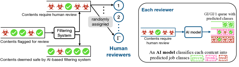
Figure 1: Schematic of a content moderation system as a triage system. Each content may be violating the user agreement (red toxicity symbol) or considered safe (green checkmark). This ground truth requires human review to uncover (“service”). Contents are flagged for review by users or automated filters, which we view as “entering” the triage system. The online platform uses an initial AI model to filter out contents most deemed to be safe. Then, remaining jobs/contents are randomly assigned to the human reviewers, a common practice due to fairness considerations in terms of mental workload. An AI model classifies each content into different classes (e.g., hate speech on a protected group), placing them in the corresponding virtual queue for the predicted class.

The random assignment assumption allows us to model the system as a set of single-server queues where job classes (e.g., toxicity) are a priori unknown. Here, misclassifications have endogenous impact on congestion since prioritizing a job delays the processing of others. To minimize the overall cost, we must balance heterogeneous service rates—such as political misinformation being harder to review than nudity—and the adverse effects of congestion, like toxic content going viral, by accounting for how misclassification errors reverberates through the queueing system.

When the class of every job is known, a simple index-based myopic policy—the oracle G$c\mu$-rule—is optimal in highly congested systems [63, 40]. Concretely, consider a single-server queue with $K$ distinct job classes with arrival and service rates $\lambda_{k}$ and $\mu_{k}$, which we assume are known to the modeler. Let $C_{k}(\cdot)$ be a convex cost function defined on sojourn time of jobs in class $k=1,\ldots,K$ (time between job arrival and service completion). The oracle G$c\mu$-rule is intuitive and simple: it greedily prioritizes jobs with the highest marginal cost of delay

$$\mathop{\rm argmax}_{k\in[K]}\mu_{k}(t)(C_{k})^{\prime}(a_{k}(t))\qquad\qquad\mbox{Oracle G$c\mu$-rule},$$ (1.1)

where $a_{k}(\cdot)$ is the age or the waiting time of the oldest unfinished job of class $k$.

When the true classes are unknown, we predict the job class using a classifier. Letting $\underline{\lambda}_{l}$ and $\underline{\mu}_{l}$ be the arrival and service rates for a predicted class $l$, a naive adaptation of the G$c\mu$-rule is

$$\mathop{\rm argmax}_{l\in[K]}\underline{\mu}_{l}(t)(C_{l})^{\prime}(\underline{a}_{l}(t))\qquad\qquad\mbox{Naive G$c\mu$-rule},$$ (1.2)

where $\underline{a}_{l}(\cdot)$ is the age or the waiting time of the oldest unfinished job with predicted class $l$ (Definition 2). This index policy does not consider misclassifications and ignores the fact that delay cost depends on the true class label instead of the predicted class: the delay cost of a content depends on whether it is toxic, rather than the prediction of toxicity. This mismatch leads to suboptimal scheduling decisions as we show in Theorem 3 to come.

We propose and analyze an index policy that optimally incorporates the impact of prediction errors in the overall cost of delay. We consider the weighted average of true class costs $C_{k}$ using the conditional probability that a job predicted as class $l$ belongs to class $k$

$$\underline{C}_{l}(t):=\sum_{k=1}^{K}\frac{p_{k}\underline{q}_{kl}}{\sum_{k^{\prime}=1}^{K}p_{k^{\prime}}\underline{q}_{k^{\prime}l}}\cdot C_{k}(t),~{}~{}~{}t\in[0,\infty),$$ (1.3)

where $p_{k}$ is the probability that an arbitrary job in the system belongs to class $k$, and $\underline{q}_{kl}$ is the probability that an arbitrary class $k$ job is predicted as class $l$. This gives rise to the index rule

$$\mathop{\rm argmax}_{l\in[K]}\underline{\mu}_{l}(t)(\underline{C}_{l})^{\prime}(\underline{a}_{l}(t))\qquad\qquad\mbox{P$c\mu$-rule},$$ (1.4)

which is easy to implement since the arrival rates and misclassification errors that determine $\underline{C}_{l}(t)$ can be efficiently estimated. In the specific case of linear delay costs and steady-state waiting time as the performance metric, the Pc$\mu$-rule bears resemblance to Argon and Ziya [4, Section 8]’s policy defined with conditional distributions of the true classes given the signal from a job. In contrast, we model increasing marginal cost of delay in content moderation through strongly convex cost functions and prove (heavy traffic) optimality over all feasible policies, in contrast to Argon and Ziya [4]’s analysis focusing on dominance over first-come-first-serve policies.

Offline deep reinforcement learning (DRL) methods are a popular contender to sequential decision-making. While flexible, DRL methods require significant engineering efforts to be reliably trained [29, 66, 16], and the performance of DRL methods is known to be highly sensitive to hyperparameters, implementation details, and even random seeds [29]. On a single-server queue with 10 classes, we observe that deep Q-learning policies with experience replay exhibits substantial variation in performance across hyperparameters, even when using identical instant rewards functions, training/testing enviroments, and same random seeds across training runs (Figure 3). The simple index policy P$c\mu$-rule significantly outperforms the best-performing DRL hyperparameter configuration (Figure 3), as we illustrate in detail in Section 5.

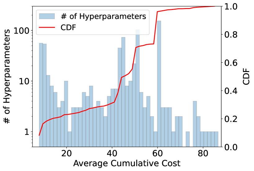
Figure 2: Histogram of average cumulative queueing cost of deep Q-learning policies over 672 hyperparameter configurations.

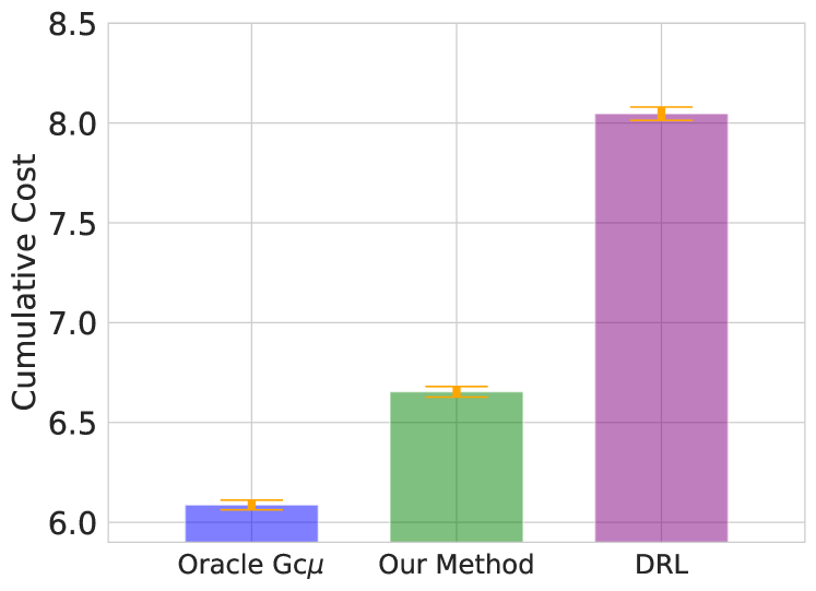
Figure 3: Cumulative cost with 2$\times$ standard errors

In contrast to the growing body of work on learning in queueing that develop online learning algorithms [13, 34, 36, 59, 65, 22], we propose an off-policy method to model applications where experimentation is risky or unwieldy. This reflects operational constraints that arise from modern AI-based service systems where models are trained offline using previously collected data. Since we assume service times are determined by true classes, in principle observed service times contain information about true class labels that can be used to improve the classifier in real time. Even in the largest industrial scenarios, however, online learning requires prohibitive infrastructure due to the high engineering complexity required for implementation. Any prediction model must be thoroughly validated prior to deployment, and the timescale for model development is typically longer (weeks to months) than that for scheduling decisions (hours to days). We thus view our offline heavy traffic analysis to be an useful analytic device for modeling AI-based queueing systems that operate close to system capacity. See Section 8 for a thorough literature review.

Contributions

Our work contributes to the growing literature studying the interface between predictive models and decision-making [4, 41, 57, 33, 12, 60]. Prediction is rarely the end goal in operational scenarios, but the link between predictive performance and downstream decision-making performance is complex due to endogeneity—misclassifications have downstream impact on delays. This work crystallizes how classical tools from queueing theory can be modified to provide managerial insights on the control and design of AI-based service systems.

Since solving for the optimal scheduling policy is computationally intractable even when job classes are known due to large state/policy spaces [46], we study highly congested systems in the heavy traffic limit as is standard in the queueing literature [50, 63, 28, 68, 40]. Our theoretical framework characterizes the optimal queueing performance in the presence of misclassification errors (Sections 3, 4), and offers several insights on the design of AI-based service systems like the one we study in Figure 1. Along the way, we identify a number of technical errors in the classical framework [63] and identify conditions under which prior results hold by giving corrected proofs based on our new techniques.

First, we derive a simple scheduling algorithm (1.4) with strong optimality and robustness guarantees by analyzing the stochastic fluctuations in the queue lengths of the unobservable true class jobs, and aggregating them to represent the fluctuation in the queue length of each predicted class (Section 3). We quantify the optimal workload allocation across the predicted classes and derive the P$c\mu$ cost function from the KKT conditions of the optimal resource allocation problem in the heavy traffic limit (3.4) (Section 4). Our theoretical results show that the P$c\mu$-rule induces queueing dynamics that achieve the asymptotic optimality with exogenous costs $\underline{C}_{l}(\cdot)$.

Next, we study the design of AI models with a central focus on decision-making. Although predictive performance is rarely the final goal, models are typically validated based on predictive measures such as precision or recall for convenience. But overparameterized models (e.g., neural networks) can achieve the same predictive performance, yet exhibit very different downstream decision performance [17, 8]. We quantify the connection between predictive performance and the cost of delay, allowing us to design AI models with downstream decision-making performance as a central concern (Section 6). We propose a model selection procedure based on the cumulative queueing cost, and demonstrate its advantages in contrast to conventional model selection approaches in ML that solely rely on predictive measures.

Finally, we use our characterization of the optimal queueing cost under misclassifications to inform the design of the queueing system itself. In the context of our motivating content moderation problem, we design an AI-based triaging system that helps determine staffing levels and corresponding filtering levels based on predictions from an initial round AI model (which may or may not be the same model used to classify jobs into classes). We propose a holistic framework trading off filtering cost, predictive performance, hiring costs, and congestion in the queueing system (Section 7). Our formulation significantly contributes to the practical discussion on designing content moderation systems, which traditionally focuses on pure prediction metrics [2, 54, 67, 1]. In Section 7.4, we demonstrate that traditional prediction-based metrics may accurately reflect the overall costs of a triage system when either filtering costs or hiring costs are the predominant factor. However, these metrics fall short in more complex scenarios where there are trade-offs between different types of costs. As a result, optimizing for these metrics typically requires computationally expensive queueing simulations. In contrast, our method reliably determines the optimal staffing and filtering levels across all scenarios by simulating a (reflected) Brownian motion.

2 Model

We begin by presenting our analytic framework in the heavy traffic regime. There are two possible data generating processes we can study. We could view jobs as originating from a single common arrival process, where interarrival times are independent of job features, true classes labels, and service times. This single arrival stream allows us to disentangle the arrival and service processes of predicted classes, and directly use the diffusion limit to show optimality of the P$c\mu$-rule. On the other hand, we may consider a more general generating process where the arrival and service processes for different classes are exogenously given. In this setting, we can still show similar mathematical guarantees as under the single stream model using heavy traffic analysis techniques pioneered by Mandelbaum and Stolyar [40]. However, this proof approach weakens our optimality results: we can only show optimality of the P$c\mu$-rule over first-come-first-serve policies, whereas under the single stream model, the direct analysis allows proving optimality over all feasible policies (see Section B.4). Furthermore, this proof approach requires more restrictive regularity conditions than the direct method that is possible under the single arrival stream model—see Section E.3 for a detailed discussion. We view the practical modeling capabilities of the two data generating assumptions to be similar; the singe arrival stream is a good model of the content moderation system (as depicted in Figure 1). Henceforth, we thus focus on the single common arrival process for expositional clarity and crisp mathematical results.

We consider a sequence of single-server multi-class queueing systems indexed by $n\in\mathbb{N}$, connected through a heavy traffic condition. Each system $n$ operates on a finite time horizon $[0,n]$, and starts empty. Let $u_{i}^{n}$ be i.i.d. interarrival times with an arrival rate $\lambda^{n}$. For $t\in[0,n]$, let $U_{0}^{n}(t):=\sum_{i=1}^{\lfloor t\rfloor}u_{i}^{n}$ be the arrival time of the $\lfloor t\rfloor$th job in the system and $A_{0}^{n}(t)=\max\{m:U_{0}^{n}(m)\leq t\}$ be the total number of jobs that arrive up to time $t$. For each class $k$, let $p_{k}^{n}:=\mathbb{P}^{n}[Y_{1k}^{n}=1]$ be the class prevalence and $(\mu_{k}^{n})^{-1}:=\mathbb{E}^{n}[v_{1}^{n}\mid Y_{1k}^{n}=1]$ the expected service time. For each job, a tuple $(X_{i}^{n},Y_{i}^{n},v_{i})$ is generated independently of its interarrival time $u_{i}^{n}$ where $X_{i}^{n}\in\mathbb{R}^{d}$ represents the feature vector associated with the $i$th job, $v_{i}^{n}$ indicates the time required to serve the $i$th job, and $Y_{i}^{n}=(Y_{i1}^{n},...,Y_{iK}^{n})$ denotes the one-hot encoded representation of its true class label. Let $V_{0}^{n}(t):=\sum_{i=1}^{\lfloor t\rfloor}v_{i}^{n},~{}\forall~{}t\in[0,n]$ be the total service time required by the first $\lfloor t\rfloor$ jobs.

A classifier $f_{\theta}$ predicts a class for each job $i$ using observed features $X_{i}^{n}$, and the job $i$ joins the (virtual) queue corresponding to the (one-hot encoded) predicted class $\underline{Y}_{i}^{n}:=f_{\theta}(X_{i}^{n})$ to wait for service. Let $\underline{q}_{kl}^{n}:=\mathbb{P}^{n}[\underline{Y}_{1l}^{n}=1\mid Y_{1k}^{n}=1]$ be the probability of a class $k$ job being predicted as class $l$; $Q^{n}:=(\underline{q}_{kl}^{n})_{k,l\in[K]}$ is the confusion matrix.

We assume service time is conditionally independent of the covariates given the true class label $Y^{n}_{i}$, $v_{i}^{n}\perp X^{n}_{i}\mid Y^{n}_{i}$, which simplies our anlysis by only considering true class label’s impact on service time. In practice, if covariates influence service time (e.g., content length), we can mitigate such dependency by creating more fine-grained true classes. We summarize our data generating process as in the following assumption.

Assumption A (Data Generating Processes).

For any system $n\in\mathbb{N}$, i) $\{(u_{i}^{n},v_{i}^{n},X_{i}^{n},Y_{i}^{n}):i\in\mathbb{N}\}$ is a sequence of i.i.d. random vectors, ii) $\{u_{i}^{n}:i\in\mathbb{N}\}$ and $\{(v_{i}^{n},X_{i}^{n},Y_{i}^{n}):i\in\mathbb{N}\}$ are independent, and iii) for any $i\in\mathbb{N}$, $v^{n}_{i}$ and $X^{n}_{i}$ are conditionally independent given $Y^{n}_{i}$.

The following assumption formalizes the notion of heavy traffic.

Assumption B (Heavy Traffic Condition).

Given a classifier $f_{\theta}$ and a sequence of queueing systems, there exist $p_{k},\underline{q}_{kl}\in[0,1]$ and $\lambda,\mu_{k}$ such that $\sum_{k=1}^{K}p_{k}\underline{q}_{kl}>0$, $\lambda\sum_{k=1}^{K}\frac{p_{k}}{\mu_{k}}=1$, and

$$n^{1/2}\big{(}\lambda^{n}-\lambda\big{)}\rightarrow 0,\quad n^{1/2}\big{(}\mu_{k}^{n}-\mu_{k}\big{)}\rightarrow 0,\quad n^{1/2}\big{(}p_{k}^{n}-p_{k}\big{)}\rightarrow 0,\quad n^{1/2}\big{(}\underline{q}_{kl}^{n}-\underline{q}_{kl}\big{)}\rightarrow 0.$$ (2.1)

$\lambda^{n}-\lambda=o(n^{-1/2})$ and $\mu_{k}^{n}-\mu_{k}=o(n^{-1/2})$ aligns with classical assumptions [40, Eq. (2)], and as usual we have that traffic intensity $\rho^{n}:=\lambda^{n}\sum_{k}p_{k}^{n}/\mu_{k}^{n}$ converges to $1$ at $o(n^{-1/2})$-rate

$$n^{1/2}[\rho^{n}-1] =n^{1/2}\Big{[}\lambda^{n}\sum\limits_{k=1}^{K}\frac{p_{k}^{n}}{\mu_{k}^{n}}-1\Big{]}\rightarrow 0.$$ (2.2)

The convergence rates in Assumption B are necessary for the results in Theorem 2 and Theorem 3 to come.

Notation

Let $\mathcal{C}$ be the space of continuous $[0,1]\mapsto\mathbb{R}$ functions, $\mathcal{D}$ the set of the right-continuous with left limits (RCLL); all stochastic processes will be RCLL. Let $\mathcal{D}^{k}$ be its product space and $\|\mathbf{x}(t)\|:=\max_{i\in[k]}|x_{i}(t)|$. Define $d_{J_{1}}(\cdot,\cdot):\mathcal{D}\times\mathcal{D}\rightarrow\mathbb{R}_{+}$ to be the $J_{1}$ (Skhorohod) metic [68, Page 79]. For any vector-valued functions $\mathbf{x}(t),\mathbf{y}(t)\in\mathcal{D}^{k}$, define $d_{p}(\mathbf{x},\mathbf{y})=\sum_{i=1}^{k}d_{J_{1}}(x_{i},y_{i})$ [68, Page 83] and its topology $WJ_{1}$ (weak $J_{1}$ topology). For a stochastic process, $A^{n}_{k}(t)$, the underlined format is used to denote the counterpart process associated with the predicted class, $\underline{A}^{n}_{l}(t)$.

3 Lower bound on queueing cost

Our analysis relies on a diffusion limit for predicted classes of the model. Scheduling is based on predicted classes, but service times are determined by the true classes. We characterize how misclassifications incur externalities on other jobs, and derive the optimal queueing cost in Theorem 2 to come. Compared to classical results in queueing that assume job classes are known [63, Proposition 6], our analysis requires handling the unobservable queue lengths of true classes as mentioned earlier; see the discussion in Section C.1.

When the job classifier is “perfect”, we have $Q^{n}=I$ where $Q^{n}$ is the confusion matrix defined in the previous section. In this case, our setting reduces to the classical setting where true classes are known, and our proofs to come give the counterpart results in Van Mieghem [63] and Mandelbaum and Stolyar [40]. Even in this classical setting, our analysis identifies missing assumptions (e.g., the zero limits in Assumption B) and provides proofs of missing arguments in Van Mieghem [63], Mandelbaum and Stolyar [40].

3.1 Convergence of endogenous processes

Define the counting processes for arrivals and service completions in the predicted classes. Let the $l$-th component of $\underline{\mathbf{A}}^{n}:[0,n]\rightarrow\mathbb{N}^{K}$ be the number of jobs that are predicted as class $l$ until time $t\in[0,n]$, and similarly let $\underline{\mathbf{S}}^{n}:[0,n]\rightarrow\mathbb{N}^{K}$ count service completions as a function of the total time that the server dedicates to each predicted class. Let $\underline{\mu}_{l}^{n}$ be the service rate of jobs in predicted class $l$, with $\underline{\mu}_{l}$ as the corresponding limit. For ease of exposition, we defer a formal discussion of diffusion limits Section A and defer precise definitions to Section B.3.

Feasible Policies

A scheduling policy $\text{$\pi$}_{n}$ is characterized by an allocation process $\underline{\mathbf{T}}^{n}:[0,n]\rightarrow\mathbb{R}^{K}$ whose $l$-th coordinate denotes the total time dedicated to predicted class $l$ up to $t\in[0,n]$. We use $\text{$\pi$}_{n}$ and $\underline{\mathbf{T}}^{n}$ interchangably. Let $\underline{\mathbf{N}}^{n}(t):[0,n]\rightarrow\mathbb{N}^{K}$ be the queue length process; its $l$-th coordinate denotes total jobs from predicted class $l$ remaining in system at $t\in[0,n]$. Let $I^{n}(t):=t-\sum_{l}\underline{T}^{n}_{l}(t)$ be the cumulative idling time up to $t\in[0,n]$. The scheduler has full knowledge of arrivals and the queue of predicted classes.

Definition 1 (Feasible Policies).

The sequence of scheduling policies $\{\text{$\pi$}_{n}\}$ is feasible if the associated processes $\{\underline{\mathbf{T}}^{n}(t),\underline{\mathbf{N}}^{n}(t),I^{n}(t)\}$ satisfy for all $n\in\mathbb{N}$,

1. $\underline{\mathbf{T}}^{n}(0)=\mathbf{0}$, $\underline{\mathbf{T}}^{n}$ is continuous and nondecreasing, $\underline{\mathbf{N}}^{n}\geq 0$, and $I^{n}$ is nondecreasing;

2. $\{\underline{\mathbf{T}}^{n}(t),t\in[0,n]\}$ is adapted to the filtration $\sigma\{(\underline{\mathbf{A}}^{n}(s),\underline{\mathbf{N}}^{n}(s)):0\leq s<t\}$.

Condition (i) is natural, and condition (ii) ensures that $\{\pi_{n}\}$ only relies on arrivals and queue status of predicted classes up to time $t$. We allow preemption (preemptive-resume policy) so that the server is able to pause serving one job and switch to another in a different predicted class. Preemption is not allowed between jobs from the same predicted class, consistent with classical settings [40].

Cumulative Queueing Cost

Our goal is to minimize the cumulative queueing cost determined by true class labels. For a true class $k$ job, its queueing cost is $C_{k}^{n}(\tau)$ where $\tau$ is sojourn time. Let $\underline{\tau}_{lj}^{n}$ be the sojourn time of the $j$th job of predicted class $l$, and $\underline{\boldsymbol{\tau}}^{n}=\{\underline{\tau}^{n}_{l}\}_{l\in[K]}$ be the sojourn time process tracking that of the most recently arriving job in predicted class $l$ by time $t$, i.e., $\underline{\tau}^{n}_{l}(t)=\underline{\tau}^{n}_{l\underline{A}_{l}^{n}(t)}$. Since $(\underline{\tau}_{l}^{n})_{l\in[K]}$ is of order $n^{1/2}$ (see Proposition 1 to come), we also assume commensurate scaling on $\{C^{n}_{k}\}_{k\in[K]}$ in Assumption C.

Assumption C (Cost functions I).

For all $k\in[K]$, $C_{k}^{n}(\cdot)$ is differentiable, nondecreasing, and convex for all $n$. There exists a continuously differentiable and strictly convex function $C_{k}$ with $C_{k}^{\prime}(0)=0$ such that $C_{k}^{n}(n^{1/2}\cdot)\rightarrow C_{k}(\cdot)$ and $n^{1/2}(C^{n}_{k})^{\prime}(n^{1/2}\cdot)\rightarrow C^{\prime}_{k}(\cdot)$ uniformly on compact sets.

The scaled cumulative cost function incurred by $\pi_{n}$ is

$$\tilde{J}^{n}_{\text{$\pi_{n}$}}(t;Q^{n})=n^{-1}\sum\limits_{l=1}^{K}\sum\limits_{k=1}^{K}\int_{0}^{nt}C_{k}^{n}(\underline{\tau}_{l}^{n}(s))\mathrm{d}\underline{A}_{kl}^{n}(s),~{}\forall~{}t\in[0,1],$$ (3.1)

where $\mathrm{d}\underline{A}_{kl}^{n}$ is the the Lebesgue-Stieltjes measure induced by $\underline{A}_{kl}^{n}$. $\tilde{J}^{n}_{\text{$\pi_{n}$}}(t;Q^{n})$ relies on the scheduling policy via the sojourn time process $\{\underline{\tau}^{n}_{l}\}$. Similar to the classical settings [63, 40], we study p-FCFS policies—those serving each predicted class in a first-come-first-served manner. Given a feasible policy $\pi_{n}$, we can reorder service within each predicted class to derive a feasible p-FCFS counterpart, $\text{$\pi$}_{n,\text{p-FCFS}}$, which dominates the original policy stochastically, i.e., $\mathbb{P}^{n}[\tilde{J}^{n}_{\text{$\pi$}_{n,\text{p-FCFS}}}(t)>x]\leq\mathbb{P}^{n}[\tilde{J}^{n}_{\text{$\pi_{n}$}}(t)>x],~{}\forall~{}x\in\mathbb{R},~{}t\in[0,1]$ (see Lemma 11). Since the objective (3.1) does not include preemption cost like [63, 40], work-conserving policies—the server never idles when jobs are present—dominates non-work-conserving policies in cumulative cost $\tilde{J}^{n}$ a.s. (see Lemma 12). Thus, we henceforth focus on p-FCFS and work-conserving feasible policies.

Sample path analysis

Let $\tilde{U}_{0}^{n},\tilde{V}_{0}^{n}$ be diffusion-scaled versions of partial sums of interarrival and service times:

$$\tilde{U}_{0}^{n}(t)=n^{-1/2}[U_{0}^{n}(nt)-(\lambda^{n})^{-1}\cdot nt],\quad\tilde{V}_{0}^{n}(t)=n^{-1/2}[V_{0}^{n}(nt)-\sum_{k=1}^{n}\frac{p^{n}_{k}}{\mu^{n}_{k}}\cdot nt],\quad t\in[0,1].$$ (3.2)

In Lemma 3 to come, we show there exist Brownian motions $(\tilde{U}_{0},\tilde{V}_{0})$ such that $(\tilde{U}_{0}^{n},\underline{\tilde{V}}_{0}^{n})\Rightarrow(\tilde{U}_{0},\underline{\tilde{V}}_{0})$ in $(D^{2},WJ_{1})$. Building off of our diffusion limit, we can strengthen the convergence to the uniform topology using standard tools (e.g., see Lemma 6 and Lemma 7), and conduct a sample path analysis where we construct copies of $(\tilde{U}_{0}^{n},\tilde{V}_{0}^{n})$ and $(\tilde{U}_{0},\tilde{V}_{0})$ that are identical in distribution with their original counterparts and converge almost surely under a common probability space. With a slight abuse of notations, we use the same notation for the newly construced processes.

Sample path analysis allows us to leverage properties of uniform convergence and significantly simplifies our analysis. All subsequent results and their proofs in the appendix, will be established on the copied processes in the common probability space $(\Omega_{\text{copy}},\mathcal{F}_{\text{copy}},\mathbb{P}_{\text{copy}})$ with probability one, i.e., $\mathbb{P}_{\text{copy}}\text{-}a.s.$, and all of the convergence results will be understood to hold in the uniform norm $\|\cdot\|$. For instance, Lemma 3 can be strengthen to $(\tilde{U}_{0}^{n},\underline{\tilde{V}}_{0}^{n})\Rightarrow(\tilde{U}_{0},\underline{\tilde{V}}_{0})$ in $(D^{2},\|\cdot\|)$, $\mathbb{P}_{\text{copy}}-a.s.$ as shown in Lemma 4. Also, in Lemma 10 to come, the diffusion-scaled process for $A_{0}^{n}$ converges to $\tilde{A}_{0}$ in $(D^{2},WJ_{1})$, $\mathbb{P}_{\text{copy}}-a.s.$, where $\tilde{A}_{0}$ a function of $\tilde{U}_{0}$. In addition, since these newly constructed processes are identical in distribution with their original counterparts, all subsequent results regarding almost sure convergence for the copied processes can be converted into corresponding weak convergence results for the original processes; see more discussion in Theorems 2 and 3.

Convergence of the Endogenous processes

Let $\underline{\mathbf{W}}^{n}:[0,n]\rightarrow\mathbb{R}^{K}$ be the remaining workload process representing the service requirement of remaining—waiting or being served—jobs predicted as class $l$ at $t\in[0,n]$. Then, $W_{+}^{n}(t)=\sum_{l}\underline{W}_{l}^{n}(t)$ is the total remaining workload. Let $\tilde{W}_{+}^{n}$, $\underline{\tilde{\mathbf{W}}}^{n}$, $\underline{\tilde{\boldsymbol{\tau}}}^{n}$, and $\underline{\tilde{\mathbf{N}}}^{n}$ be the diffusion-scaled processes corresponding to $W_{+}^{n}$, $\underline{\mathbf{W}}^{n}$, $\underline{\boldsymbol{\tau}}^{n}$, and $\underline{\mathbf{N}}^{n}$.

Proposition 1 (Fundamental Convergence Results).

Under Assumptions A, B, and H, and any work-conserving p-FCFS feasible policy

1. (Invariant Convergence) $\tilde{W}_{+}^{n}\rightarrow\tilde{W}_{+}:=\phi\Big{(}\tilde{V}_{0}\circ\lambda e+\sum_{k=1}^{K}\frac{p_{k}}{\mu_{k}}\tilde{A}_{0}\Big{)}$, where $\phi$ is the reflection mapping as defined in [68, Page 140, (2.5)];

2. (Equivalence of Convergence) For any predicted class $l\in[K]$, $\limsup_{n}\|\underline{\tilde{T}}_{l}^{n}\|$, $\limsup_{n}\|\underline{\tilde{N}}_{l}^{n}\|$, $\limsup_{n}\|\underline{\tilde{\tau}}_{l}^{n}\|$, and $\limsup_{n}\|\underline{\tilde{W}}_{l}^{n}\|$ are all bounded for any predicted class $l\in[K]$. Moreover, if any of the processes $\underline{\tilde{T}}_{l}^{n},\underline{\tilde{N}}_{l}^{n},\underline{\tilde{\tau}}_{l}^{n},$ or $\underline{\tilde{W}}_{l}^{n}$ converges, then all of $\underline{\tilde{T}}_{l}^{n},\underline{\tilde{N}}_{l}^{n},\underline{\tilde{\tau}}_{l}^{n},$ and $\underline{\tilde{W}}_{l}^{n}$ converge.

Proposition 1 extends the classical results of Van Mieghem [63, Proposition 2] by relaxing the assumption that true classes are known. When true classes are known, convergence for arrival and service processes of true classes ($\tilde{\mathbf{A}}^{n}$ and $\tilde{\mathbf{S}}^{n}$) can be derived directly via the the Functional Central Limit Theorem (FCLT) [63, Assumption 1]. In comparison, our generalization requires novel analysis approaches to establish convergence of diffusion-scaled arrival and service processes of predicted classes ($\underline{\tilde{\mathbf{A}}}^{n}$ and $\underline{\tilde{\mathbf{S}}}^{n}$) in Proposition 6. Specifically, we exploit the joint convergence result in Lemma 4 and characterize how misclassifications impact each subprocess. We develop novel connections from the primitives $\underline{\tilde{\mathbf{Z}}}^{n}$ and $\underline{\tilde{\mathbf{R}}}^{n}$ to $\underline{\tilde{\mathbf{A}}}^{n}$ and $\underline{\tilde{\mathbf{S}}}^{n}$, which involves techniques of random time change and continuous mapping approach. We give the full proof in Section B.1.

3.2 Asymptotic lower bound of the scaled delay cost function

We are now ready to present the main result of this section, the asymptotic lower bound for the cumulative queueing cost in the heavy traffic limit. Our lower bound motivates the design of the P$c\mu$-rule in Section 4. For predicted class $l\in[K]$, we let $\underline{\rho}_{l}:=\sum_{k}\frac{\lambda p_{k}\underline{q}_{kl}}{\mu_{k}}>0$ (Assumption B).

Theorem 2 (Heavy-traffic lower bound).

Given a classifier $f_{\theta}$ and a sequence of queueing systems, suppose that Assumptions A, B, C, and H hold. Under any feasible scheduling policies $\{\text{$\pi_{n}$}\}$, the associated sequence of cumulative costs $\{\tilde{J}^{n}_{\text{$\pi_{n}$}}(\cdot;Q^{n}):n\in\mathbb{N}\}$ satisfies

$$\liminf_{n\rightarrow\infty}\tilde{J}^{n}_{\text{$\pi_{n}$}}(t;Q^{n})\geq\tilde{J}^{*}(t;Q):=\sum_{k=1}^{K}\sum_{l=1}^{K}\int_{0}^{t}\lambda p_{k}\underline{q}_{kl}C_{k}\Big{(}\frac{\big{[}h\big{(}\tilde{W}_{+}(s)\big{)}\big{]}_{l}}{\underline{\rho}_{l}}\Big{)}\mathrm{d}s,~{}\forall t\in[0,1],$$ (3.3)

$\mathbb{P}_{\text{copy}}\text{-}a.s.,$ where $h(r)$ is an optimal solution to the following resource allocation problem

$$\text{Opt}(r):= \min_{x} \sum\limits_{l=1}^{K}\sum\limits_{k=1}^{K}\lambda p_{k}\underline{q}_{kl}C_{k}\Big{(}\frac{x_{l}}{\underline{\rho}_{l}}\Big{)}$$ (3.4)

s.t. $$\sum\limits_{l=1}^{K}x_{l}=r,\quad x_{l}\geq 0,~{}\forall~{}l\in[K].$$

Moreover, for the original processes under $\mathbb{P}^{n}$, under any feasible policies $\{\pi^{\prime}_{n}\}$,

$$\liminf_{n\rightarrow\infty}\mathbb{P}^{n}[\tilde{J}^{n}_{\pi^{\prime}_{n}}(t;Q^{n})>x]\geq\mathbb{P}_{\text{copy}}[\tilde{J}^{*}(t;Q)>x],~{}\forall~{}x\in\mathbb{R},~{}\forall~{}t\in[0,1].$$ (3.5)

According to Proposition 1, $\tilde{W}_{+}$ is solely determined by the exogenous processes $\tilde{A}_{0}$ and $\tilde{V}_{0}$. Consequently, the lower bound in Theorem 2 is independent of the scheduling policy $\underline{\mathbf{T}}^{n}$. Our proof is involved and deferred to Section C, where we also contrast our analytic approach to classical proof techniques.

4 Heavy-traffic optimality of the P$c\mu$-rule

We are ready to formally derive the P$c\mu$-rule, which is motivated by the convex optimization problem (3.4). We prove heavy traffic optimality of the P$c\mu$-rule by showing that it attains the lower bound in Theorem 2. Our result (Theorem 3) extends the classical result in Van Mieghem [63, Proposition 7].

While not the main contribution of this work, our analytic framework extend the standard heavy traffic analysis techniques [63, 40] in subtle ways as we detail in Sections E.2 and E.3. Even when specialized to the classical setting of known true classes, our analysis fills gaps in classical proofs for the optimality of the G$c\mu$-rule [63] and $D\text{-}Gc\mu$ [40]. The two methods use ages of waiting jobs, but only establish optimality stated in terms of the sojourn times. To bridge this gap, we provide a rigorous proof in Proposition 13. The proof of the proposition is nontrivial (to us) and reveals a necessary condition that was previously unstated in [63]: strong convexity of the cost functions. Also, our analysis circumvents the stronger assumptions on the cost functions in [40] in the single-server case by directly analyzing the age dynamics. See Sections E.3 for details.

We first characterize the limiting cumulative cost of a convergent policy. Let let $\underline{\bar{A}}_{kl}$ be the limit of $n^{-1}\underline{A}^{n}_{kl}(n\cdot)$ (see Definition 10 for a formal statement). In the following, $\tilde{J}_{\text{$\pi$}}(t;Q)$ is dependent on $\underline{\tilde{\boldsymbol{\tau}}}=\{\underline{\tilde{\tau}}_{l}\}_{l\in[K]}$ through the subscript $\pi$.

Lemma 1 (Convergence of $\tilde{J}^{n}_{\text{$\pi_{n}$}}(\cdot;Q^{n})$).

Given a classifier $f_{\theta}$, suppose that Assumption A, B, C, and H hold. For feasible policies $\{\text{$\pi_{n}$}\}$ satisfying $\underline{\tilde{\tau}}^{n}_{l}\rightarrow\underline{\tilde{\tau}}_{l},~{}\forall~{}l\in[K]$,

$$\sup\limits_{t\in[0,1]}|\tilde{J}^{n}_{\text{$\pi_{n}$}}(t;Q^{n})-\tilde{J}_{\text{$\pi$}}(t;Q)|\rightarrow 0,$$ (4.1)

where the limiting cumulative cost $\tilde{J}_{\text{$\pi$}}(t;Q)$ is defined by

$$\tilde{J}_{\text{$\pi$}}(t;Q):=\sum\limits_{l=1}^{K}\sum\limits_{k=1}^{K}\int_{0}^{t}C_{k}(\underline{\tilde{\tau}}_{l}(s))\mathrm{d}\underline{\bar{A}}_{kl}(s)=\sum\limits_{l=1}^{K}\sum\limits_{k=1}^{K}\int_{0}^{t}\lambda p_{k}\underline{q}_{kl}C_{k}(\underline{\tilde{\tau}}_{l}(s))~{}\mathrm{d}s.$$

See Section B.5 for the proof.

Combining our characterization of the cumulative cost with the lower bound in Theorem 2, we conclude that $\{\text{$\pi_{n}$}\}$ is asymptotically optimal if the following conditions are satisfied: i) the scaled sojourn time processes converge, i.e., $\underline{\tilde{\tau}}_{l}^{n}\rightarrow\underline{\tilde{\tau}}_{l},~{}\forall~{}l\in[K]$, and ii) the limiting sojourn time processes satisfy $\underline{\tilde{\tau}}_{l}(t)=[h(\tilde{W}_{+}(t))]_{l}/\underline{\rho}_{l},~{}\forall~{}t\in[0,1],~{}l\in[K]$, where $h(\cdot)$ is an optimal solution to the optimization problem (3.4). Recalling $\text{Opt}(\tilde{W}_{+}(t))$, the optimization problem (3.4), is convex with linear constraints, its KKT conditions characterize the optimal workload allocation $h$. For predicted class $l$, recall its limiting service rate $\underline{\mu}_{l}$ and the P$c\mu$ cost function (1.3).

Lemma 2 (KKT conditions).

$\{x_{l}\}_{l\in[K]}$ is an optimal solution for $\text{Opt}(\tilde{W}_{+}(t))$ if $x_{l}>0,~{}\forall~{}l\in[K]$ and is a solution to

$$\underline{\mu}_{l}\underline{C}_{l}^{\prime}\Big{(}\frac{x_{l}}{\underline{\rho}_{l}}\Big{)}=\underline{\mu}_{m}\underline{C}_{m}^{\prime}\Big{(}\frac{x_{m}}{\underline{\rho}_{m}}\Big{)},~{}\forall~{}l,m\in[K],\quad\sum\limits_{l=1}^{K}x_{l}=\tilde{W}_{+}(t).$$ (4.2)

We also show that the KKT conditions (4.2) have a unique solution (Proposition 15, Section C) and thus $h(\tilde{W}_{+}(t))$ is well-defined.

The cost function $\underline{C}_{l}(t)$ (1.3) arises from the KKT conditions of $\text{Opt}(\tilde{W}_{+}(t))$ as a weighted average with weights proportional to $p_{k}\underline{q}_{kl}$, reflecting how predicted class $l$ is composed of jobs from different true classes. As $p_{k}$ and $\underline{q}_{kl}$ rely on the arrival rates and misclassification errors, $\underline{C}_{l}(t)$ can be viewed as the exogenous average cost function associated with predicted class $l$. We aim to develop a scheduling policy that induces the workload allocation to align with the exogenous cost $\underline{C}_{l}(t)$, in the sense that the conditions (4.2) are satisfied for all $t\in[0,1]$.

According to Proposition 1, convergence of the sojourn time process $\underline{\tilde{\boldsymbol{\tau}}}^{n}\rightarrow\underline{\tilde{\boldsymbol{\tau}}}$ is equivalent to convergence of workload $\underline{\tilde{\mathbf{W}}}^{n}\rightarrow\underline{\tilde{\mathbf{W}}}$. Moreover, if $\underline{\tilde{\mathbf{W}}}^{n}$ converges, then $\underline{\tilde{\tau}}_{l}=\underline{\tilde{W}}_{l}/\underline{\rho}_{l},\forall~{}l\in[K]$ (see Lemma 8 and Lemma 16). Consequently, our goal is to develop a policy that satisfies $\underline{\tilde{\boldsymbol{\tau}}}^{n}\rightarrow\underline{\tilde{\boldsymbol{\tau}}}$ and

$$\underline{\mu}_{l}\underline{C}^{\prime}_{l}(\underline{\tilde{\tau}}_{l})=\underline{\mu}_{m}\underline{C}^{\prime}_{m}(\underline{\tilde{\tau}}_{m}),~{}\forall~{}l,m\in[K],$$ (4.3)

in the heavy traffic limit. When the balance (4.3) is achieved, the limiting workload allocation $\underline{\tilde{W}}_{l}=x_{l}:=\underline{\tilde{\tau}}_{l}\underline{\rho}_{l}$ satisfies the KKT conditions (4.2) and both conditions (a) and (b) are met, which leads to the policy’s optimality.

Since the sojourn time—time between job arrival and service completion—is not observable, we substitute $\underline{\boldsymbol{\tau}}^{n}=\{\underline{\tau}_{l}^{n}\}_{l\in[K]}$ with the observable age processes.

Definition 2 (Age Process).

Given a classifier $f_{\theta}$ and feasible policies $\{\text{$\pi_{n}$}\}$, a predicted class $l$ and time $t\in[0,n]$, let $\underline{a}_{l}^{n}(t)$ be the waiting time of the oldest job in predicted class $l$ at time $t$, where a job being served is defined to be waiting in the system. Let $\underline{a}_{l}^{n}$ be the age process of the predicted class $l\in[K]$ in system $n$, and let $\underline{\tilde{a}}_{l}^{n}(t):=n^{-1/2}\underline{a}_{l}^{n}(nt),~{}t\in[0,1]$ and $\underline{\tilde{\mathbf{a}}}^{n}:=\{\underline{\tilde{a}}_{l}^{n}\}_{l\in[K]}$ be the corresponding diffusion-scaled process and its vector-valued version.

If either $\{\underline{\tilde{a}}_{l}^{n}\}_{l\in[K]}$ or $\{\underline{\tilde{\tau}}_{l}^{n}\}_{l\in[K]}$ converges, then both of the processes converge to the same limit, i.e., $\underline{\tilde{\tau}}_{l}(t)=\underline{\tilde{a}}_{l}(t),~{}\forall~{}l\in[K],t\in[0,1]$ (see Proposition 12). Thus, we can equivalently reformulate the optimality condition for sojourn time (4.3) into that with observable age processes

$$\underline{\mu}_{l}\underline{C}^{\prime}_{l}(\underline{\tilde{a}}_{l})=\underline{\mu}_{m}\underline{C}^{\prime}_{m}(\underline{\tilde{a}}_{m}),~{}\forall~{}l,m\in[K].$$ (4.4)

Heavy-Traffic Optimality

We design the P$c\mu$-rule in the prelimit systems to achieve (4.4) in the heavy traffic limit. The P$c\mu$-rule prioritizes predicted classes with the highest prelimit Pc$\mu$ index, defined as follows.

Definition 3 (P$c\mu$-rule).

Given a classifier $f_{\theta}$, for any system $n$ at time $nt$ with $t\in[0,1]$, the P$c\mu$-rule serves the oldest job in the predicted class having the maximum P$c\mu$-rule index, i.e., $l\in\arg\max_{m\in[K]}\underline{\mathcal{I}}^{n}_{m}(t)$, with preemption, where

$$\underline{\mathcal{I}}^{n}_{l}(t):=\underline{\mu}^{n}_{l}\cdot n^{1/2}(\underline{C}^{n}_{l})^{\prime}(\underline{a}_{l}^{n}(nt)),~{}\forall~{}t\in[0,1],$$ (4.5)

is the P$c\mu$-rule index for predicted class $l$ at time $nt$ in system $n$, and $\underline{C}_{l}^{n}(t):=\frac{\sum_{k}p^{n}_{k}\underline{q}^{n}_{kl}C^{n}_{k}(t)}{\sum_{k^{\prime}}p^{n}_{k^{\prime}}\underline{q}^{n}_{k^{\prime}l}},~{}t\in[0,\infty),~{}l\in[K]$, is the weighted average of $C^{n}_{k}$ and the prelimit counterpart of $\underline{C}_{l}(t)$.

The P$c\mu$-rule is a work-conserving p-FCFS policy by definition, and the $n^{1/2}$ scaling ensures a well-defined heavy traffic limit. The P$c\mu$-rule naturally allows for preemption: since we consider jobs being served as waiting in the system, the age process $a_{l}^{n}$ corresponds to the same job waiting in the queue until its service completion. We adopt preemption for analysis purposes. In particular, we can develop a non-preemptive counterpart of the P$c\mu$-rule and show its optimality using the same analytic framework.

We are now ready to present our optimality result, which shows that the cumulative queueing cost associated with the P$c\mu$-rule, $\tilde{J}^{n}_{\text{Pc$\mu$}}(\cdot;Q^{n})$, converges to the asymptotic lower bound $\tilde{J}^{*}(\cdot;Q)$. Our proof relies on the fact that the P$c\mu$-rule is a greedy method minimizing the largest difference of the P$c\mu$ indices , $\sup_{t\in[0,1]}\,\max_{l,m\in[K]}|\underline{\mathcal{I}}^{n}_{l}(t)-\underline{\mathcal{I}}^{n}_{m}(t)|$, which guarantees (Proposition 13, Section E.1)

$$\sup_{t\in[0,1]}\,\max_{l,m\in[K]}|\underline{\mathcal{I}}^{n}_{l}(t)-\underline{\mathcal{I}}^{n}_{m}(t)|\rightarrow 0.$$ (4.6)

We develop novel analysis techniques to show the convergence (4.6), which requires strong convexity of the cost function.

Assumption D (Cost functions II).

The limiting cost $C_{k}$ is strongly convex for all $k\in[K]$.

Theorem 3 (Optimality of P$c\mu$-rule).

Given a classifier $f_{\theta}$ and a sequence of queueing systems, suppose that Assumptions A, B, C, D, and H hold. Then, $\tilde{J}^{n}_{\text{Pc$\mu$}}(\cdot;Q^{n})\rightarrow\tilde{J}^{*}(\cdot;Q)$ in $(\mathcal{D},\|\cdot\|)$ $\mathbb{P}_{\text{copy}}$-a.s.. For the original processes under $\mathbb{P}^{n}$, $\tilde{J}^{n}_{\text{Pc$\mu$}}(\cdot;Q^{n})\Rightarrow\tilde{J}^{*}(\cdot;Q)$ in $(\mathcal{D},J_{1})$, and in particular, $\mathbb{P}^{n}[\tilde{J}^{n}(t;Q^{n})>x]\rightarrow\mathbb{P}_{\text{copy}}[\tilde{J}^{*}(t;Q)>x],~{}\forall~{}x\in\mathbb{R},~{}t\in[0,1].$

Our proof is highly involved so we provide a brief overview in Section E.1 and defer detailed arguments to Section D and E. Our analytic framework extends upon prior work in subtle ways; see Sections E.2 and E.3 for an in-depth discussion of our proof compared to Van Mieghem [63] and Mandelbaum and Stolyar [40].

5 Empirical demonstration of the P$c\mu$-rule

We demonstrate the effectiveness of P$c\mu$-rule on a content moderation problem using real-world user-generated text comments with the data generating process in Section 2. To operate at a massive scale, online platforms use AI models to provide initial toxicity predictions. However, these models are imperfect due to the inherent nonstationarity in the system; for example, they cannot reliably detect context related to hate speech following a recent terrorist attack. As a result, platforms must rely on human reviewers as the final inspectors [39], especially since they bear the cost of mistakenly removing non-violating comments. Our goal is to analyze the downstream impact of prediction errors on scheduling decisions in the content moderation queueing system.

Different comments incur varying levels of negative impact on the platform. If not removed in a timely manner, toxic comments attacking historically marginalized or oppressed groups can have particularly harmful effects. We model this using heterogeneous delay costs based on the level of toxicity and the demographic group targeted by the comment. These factors also affect processing time; for instance, reviewing comments about an ethnic minority group in a foreign nation is more challenging and time-consuming compared to domestic content.

We use real user-generated text comments on online articles from the CivilComments dataset [10]. Each comment has been labeled by at least ten crowdsourcing workers with binary toxicity labels and whether it mentions one of the 8 demographic identities: male, female, LGBTQ, Christian, Muslim, other religions, Black, White. For simplicity, we focus on comments that mention one and only one of the common groups white, black, male, female, LGBTQ. By crossing them with binary toxicity labels, we derive 10 job classes. We assume the system has exact knowledge of target group (using simple rule-based logic), but can only predict the toxicity through an AI model.

The toxicity predictor, which can also be viewed as the job class predictor $f_{\theta}$, utilizes the same neural network architecture and training approach as described in Koh et al. [32]. To showcase the versatility of our scheduling algorithm regardless of the underlying prediction model, we study three models fine-tuned based on a pre-trained language model (DistilBERT-base-uncased [53]): empirical risk minimization (ERM), reweighted ERM that upsamples toxic comments, and a simple distributionally robust model trained to optimize worst-group performance over target demographic groups (GroupDRO [52]). We observe significant variation in predictive performance across the 10 job classes defined by $\{$toxicity $\times$ target demographic$\}$. Across the three models (ERM, Reweighted, GroupDRO), the worst-class accuracy (55%, 68%, 67%) is significantly lower than the mean accuracy (88%, 84%, 84%), leading to diverse patterns in the confusion matrix $Q$.

Queueing system

We assume jobs are assigned to reviewers randomly to ensure fairness, as mentioned in Section 1, and view each reviewer as a single-server queueing system. For simplicity, we consider a queueing model operating in a finite time interval $[0,1]$ with 10 job classes. New jobs/comments arrive with i.i.d. exponential interarrival times with rate 100 (uniformly drawn from the test set). Toxic comments have a lower service rate and toxic comments mentioning minority groups have an even lower service rate. The service times follow exponentially distributions that solely depend on the true class label $Y$: for white, black, male, female, LGBTQ, respectively, $\mu_{\text{toxic}}=[100,30,110,25,15]$ and $\mu_{\text{non-toxic}}=[150,150,150,150,150]$. (If the service rate depends on the covariate $X$, e.g., length of the comment, we can create further classes by splitting on relevant covariates.) Our queueing system operates in heavy traffic with overall traffic intensity $\approx 1$, aligning with Assumption B. We set higher delay costs for toxic comments and coments targeting historically marginalized or oppressed groups. Specifically, for each demographic group $i$, we set the delay cost as $C_{i,\cdot}(t)=c_{i,\cdot}t^{2}/2,$ with $c_{i,\text{toxic}}=[10,22,12,20,25]$ and $c_{i,\text{non-toxic}}=[1,1,1,1,1]$ for toxic and nontoxic comments mentioning the aforementioned demographic groups, respectively.

Queueing policies

We compare our proposed P$c\mu$-rule against three scheduling approaches. First, we consider the Naive G$c\mu$-rule (1.2) that treats the predicted classes as true, and employs the usual Gc$\mu$-rule. For both P$c\mu$-rule and Naive G$c\mu$-rule, we assume the scheduler has complete knowledge of the arrival/service rates of the predicted classes, and use the confusion matrix $Q$ computed on the validation dataset. Second, we study a black-box approach scheduling using deep reinforcement learning methods (DRL), where we use a Q-learning method to estimate the value function using a feedforward neural network (deep Q-Networks [42]). Finally, we consider the Oracle Gc$\mu$ policy, which knows the true class as well as associated arrival/service rates. All policies are evaluated in the aforementioned setup, where the scheduler predicts the class label using the AI model $f_{\theta}$.

To train our DRL policy, we use Namkoong et al. [44]’s discrete event queueing simulator. We use $\{(\text{queue length, age of the oldest job})\}$ of all predicted classes as our state space and let the predicted classes $\{1,\ldots,K=10\}$ be the action space. We learn a Q-function parameterized by a three-layer fully connected network, and serve the oldest job in the predicted class that maximizes the Q-function. As instantaneous rewards, we use the sum of cost rates, $c_{i,\cdot}$ times the age, for all classes. We employ a similar training procedure as described in [44, Section D.1], and impose a large penalty to discourage the policy from serving empty queues.

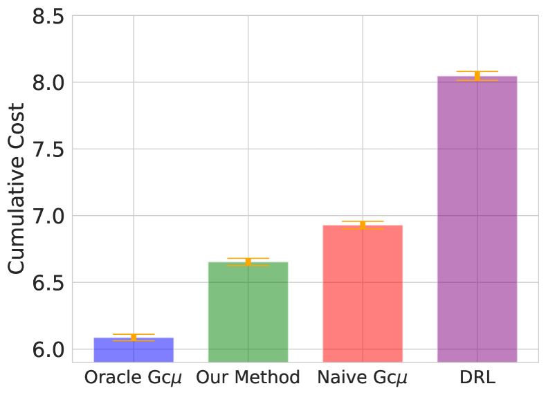
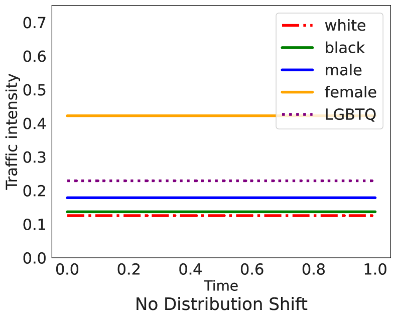
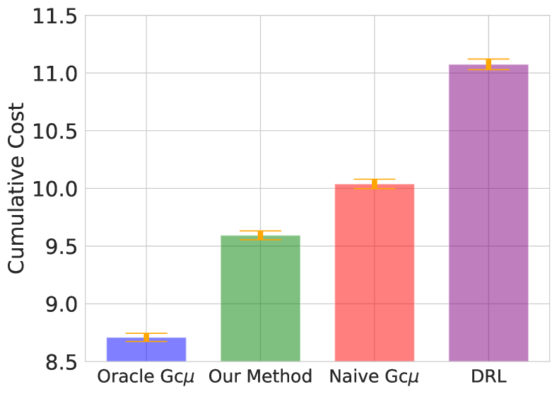
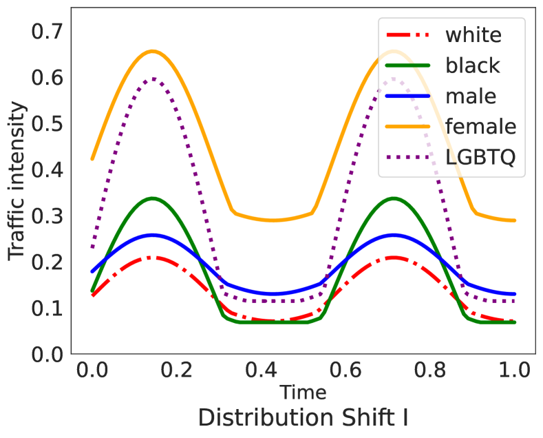
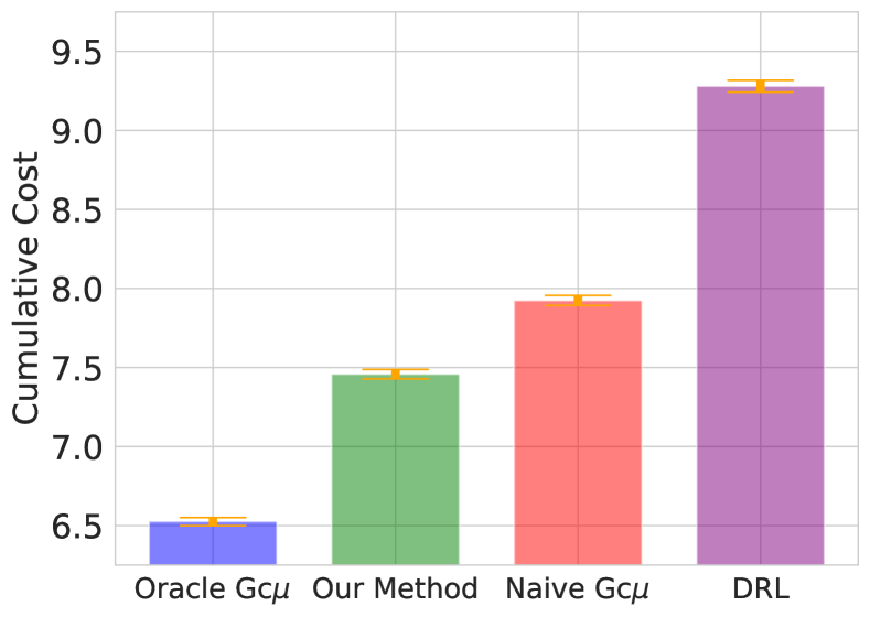
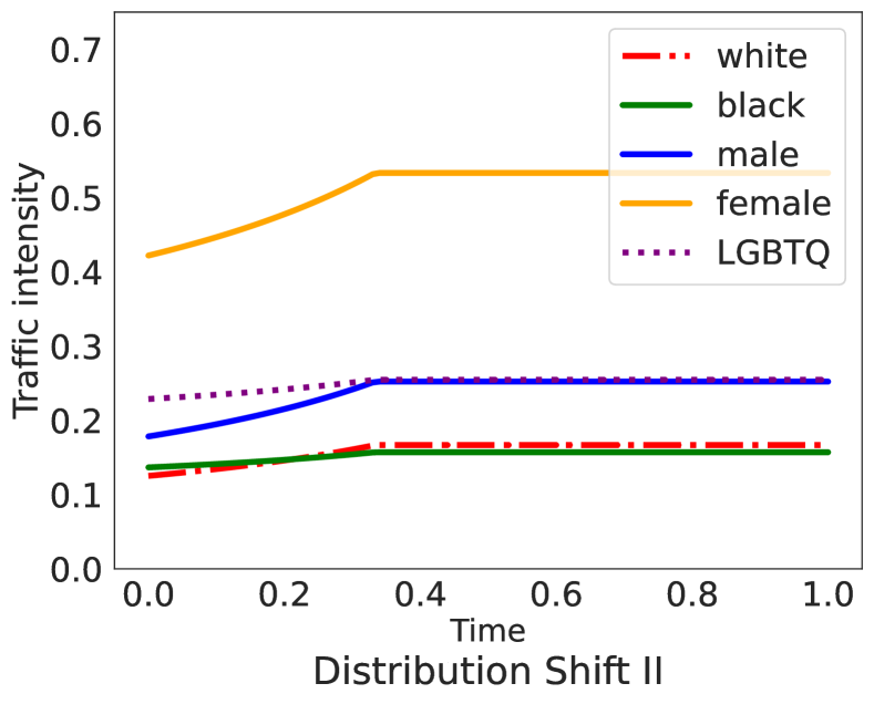
Figure 4: We present the cumulative cost for different policies under different testing environments (with 2$\times$ the standard error encapsulated in the orange bracket).

Instability of reinforcement learning

We run the deep Q-learning method with experience replay over 672 distinct sets of hyperparameters and evaluate them based on the average cumulative queuing cost over $5000$ independent sample paths simulated from the testing enviroment. In Figure 3, we observe substantial variation in queueing performance across hyperparameters even when using identical instant reward functions and training/testing enviroments. (We also use the same random seed across training runs.) In particular, the minimum, bottom & top deciles of cumulative costs are 7.98, 9.79, and 60.46. Our empirical observation highlights the significant engineering effort required to apply DRL approaches to scheduling and replicates previous findings in the RL literature (e.g., [29]). In the rest of the experiments, we select the best hyperparameter based on average queueing costs reported in Figure 3.

Main results

In Figure 4, we present cumulative cost averaged over $50K$ sample paths. In the first column of Figure 4, we test scheduling policies under the environment they were designed for: constant arrival/service rates as we described above, with traffic intensity $\approx$ 1. The P$c\mu$-rule outperforms Naive G$c\mu$-rule by $\sim 30\%$ and DRL by $60-70\%$ in terms of the cost gap towards the Oracle G$c\mu$-rule. While we expect the DRL policy can be further improved by additional engineering (reward shaping, neural network architecture search etc), we view the simplicity of our index-based policy as a significant practical advantage. Next, we assess the robustness of the scheduling policies against nonstationarity in the system. We consider two additional testing enviroments with heavy traffic conditions that differ from that the policies were designed for. We observe the performance gains of the P$c\mu$-rule hold over nonstationarities in the system.

The Pc$\mu$-rule consistently shows superior performance across different scenarios, demonstrating its robustness and practical utility in real-world content moderation tasks.

6 Model selection based on queueing cost

Predictive models with similar accuracy levels can exhibit significant differences in queueing performance. By explicitly deriving the optimal queueing cost under misclassification, our theoretical results allow designing AI models with queueing cost as a central concern. Since the P$c\mu$-rule is optimal in the heavy traffic limit, the corresponding $\tilde{J}^{*}(t;Q)$ represents the best possible cost when employing the given classifer, $f_{\theta}$, and the relative regret $\tilde{J}^{*}(t;Q)/\tilde{J}^{*}(t;I)$ serves as an evaluation metric with queueing performance as the central consideration. We empirically demonstrate that this simple model selection criteria based on our theory can provide substantial practical benefits in our content moderation simulator.

For quadratic cost functions, we can explicitly solve the optimization problem (3.4) and derive analytic expressions for $\tilde{J}^{*}(\cdot;Q)$ and $\tilde{J}^{*}(\cdot;I)$.

Assumption E (Quadratic Cost Functions).

For all $k\in[K]$, the cost functions are defined as $C^{n}_{k}(t)=\frac{1}{2n}c^{n}_{k}t^{2},~{}t\in[0,n],~{}n\in\mathbb{N}$, and $C_{k}(t)=\frac{1}{2}c_{k}t^{2},~{}t\in[0,1]$, where $\{c^{n}_{k}\}_{n\in\mathbb{N}}$ and $c_{k}$ are positive constants such that $c_{k}^{n}\rightarrow c_{k}$ as $n\rightarrow\infty.$

The following formulas are easy to approximate since the confusion matrix $Q$ can be effectively estimated on held-out data.

Proposition 4 (Cumulative Cost Rate of the P$c\mu$-rule).

Given a classifier $f_{\theta}$ and a sequence of queueing systems, suppose that Assumptions A, B, E, and H hold. Then, we have that

$$\tilde{J}^{*}(t;Q)=\frac{1}{\sum_{m=1}^{K}(\beta_{m}(Q))^{-1}}\cdot\frac{1}{2}\int_{0}^{t}\tilde{W}_{+}(s)^{2}\mathrm{d}s,~{}\forall~{}t\in[0,1],$$

where $\beta_{l}(Q):=\underline{\mu}_{l}\underline{c}_{l}/\underline{\rho}_{l}$. Under the Naive G$c\mu$-rule, the scaled cumulative queueing cost $\tilde{J}^{n}_{\text{Naive}}(\cdot;Q^{n})$ has the limit

$$\tilde{J}_{\text{Naive}}(t;Q)=\sum\limits_{l=1}^{K}\frac{\beta_{l}(Q)}{\Big{(}\sum_{m}\frac{\beta_{l,\text{Naive}}(Q)}{\beta_{m,\text{Naive}}(Q)}\Big{)}^{2}}\cdot\frac{1}{2}\int_{0}^{t}\tilde{W}_{+}(s)^{2}\mathrm{d}s,$$

where $\beta_{l,\text{Naive}}(Q)=\underline{\mu}_{l}c_{l}/\underline{\rho}_{l}$.

See Section F.1 for the proof of Proposition 4. $\tilde{J}^{*}(\cdot;Q)$ is dominated by small values of $\beta_{m}(Q)$, as is the case for the limiting workload $\underline{\tilde{W}}_{m}$ under the P$c\mu$-rule(see Section F.1). Small $\beta_{m}(Q)$ implies either high intensity or low priority of the predicted class, meaning the impact of $f_{\theta}$ is determined by the “imbalance” of $\{\beta_{m}(Q):m\in[K]\}$ between the predicted classes.

In what follows, we heavily rely on the independence between $\tilde{W}_{+}$ and misclassification errors from Proposition 1.

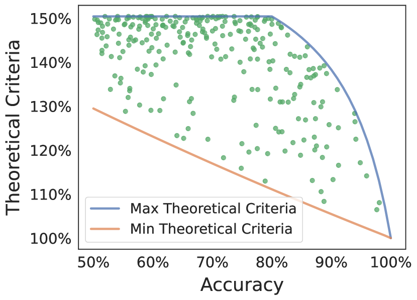
(a) High arrival rate of positive class

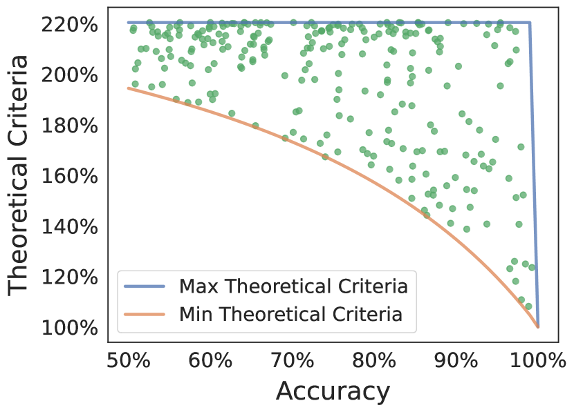
(b) Low arrival rate of positive class

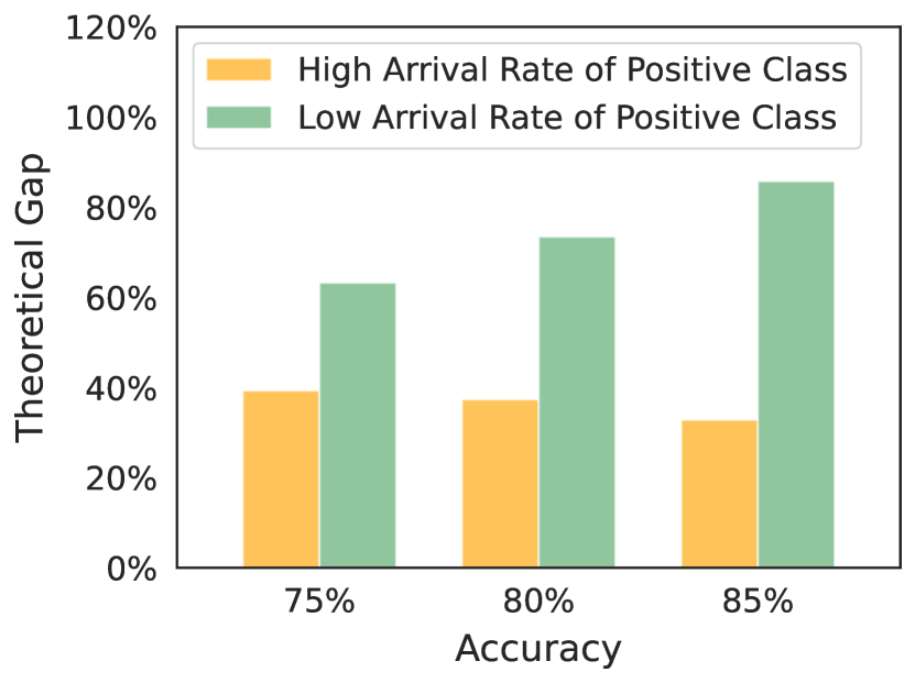
(c) Theoretical gap under different accuracy levels

Figure 5: Maximum and minimum relative regret $\tilde{J}(t;Q)/\tilde{J}^{*}(t;I)$ in the heavy traffic limit (“theoretical criteria”) across accuracy levels. Each green dot corresponds to theoretical criteria and accuracy of a simulated confusion matrix $Q$.

Model Multiplicity

It is well known that models of equal prediction accuracy can perform differently in downstream decision-making tasks [17, 8]. This phenomenon, known as model multiplicity [8], is particularly important in our setting, since prediction errors over different classes can have disproportionate impacts on downstream queueing performance. We consider a two-class toy example to showcase that models with high accuracy levels can still exhibit significant differences in queueing performances.

We simplify the setting from Section 5 to two classes: toxic comments (positive class, class 1), and non-toxic comments (negative class, class 2), where delay costs are set as $C_{k}(t)=c_{k}t^{2}/2$ with $c_{1}=15,c_{2}=1$. We examine two settings: (i) high arrival rate of the positive class, with $[\lambda_{1},\lambda_{2}]=[25,100]$, $[\mu_{1},\mu_{2}]=[50,200]$; and (ii) low arrival rate of the positive class, with $[\lambda_{1},\lambda_{2}]=[1,100]$, $[\mu_{1},\mu_{2}]=[2,200]$. The arrival and service rates are chosen to achieve an overall traffic intensity close to 1 and approximate heavy traffic limits.

Given fixed costs, arrival rates, and service rates, we can explcitly quantify the relative regret $\tilde{J}^{*}(t;Q)/\tilde{J}^{*}(t;I)$ for different classifiers through the confusion matrix $Q$, considering the maximum and minimum possible relative regret given a fixed accuracy level. In Figure 5(a)-(b), we study systems with two different arrival rates. We randomly generate 500 confusion matrix $Q$ ($\underline{q}_{11},\underline{q}_{22}\stackrel{{\scriptstyle\rm iid}}{{\sim}}\mbox{Unif}[0,1]$) and plot the resulting accuracy level and theoretical criteria in green dots. The variation in relative regret is substantial in both settings, and in Figure 5(c), even at high accuracy levels ($75\%,80\%,85\%$), the relative regret can vary by $30\%$ to $80\%$. This indicates that model multiplicity significantly affects queuing performance, which highlights the potential of using our evaluation metric in guiding model selection.

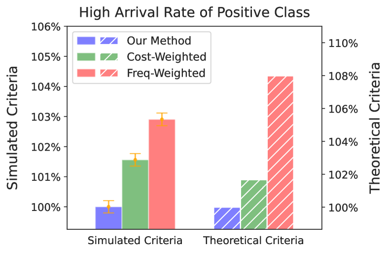
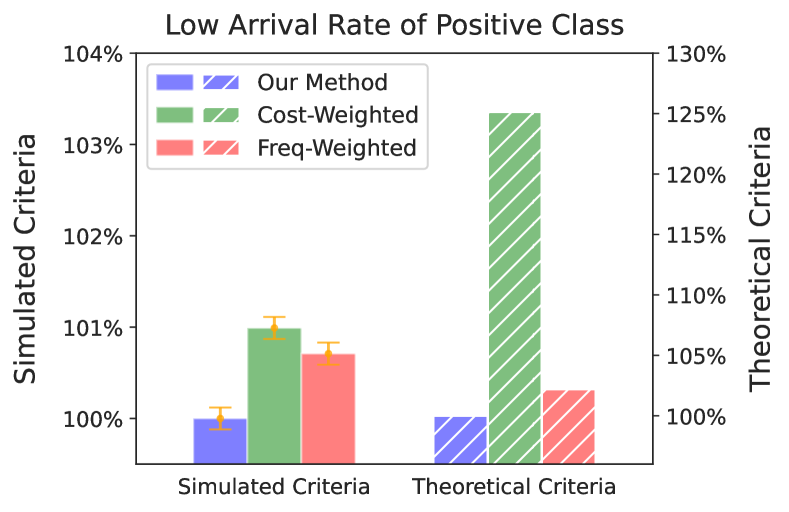
(a) threshold selection for a fixed classifer

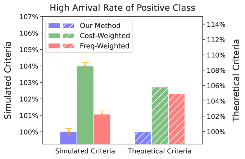
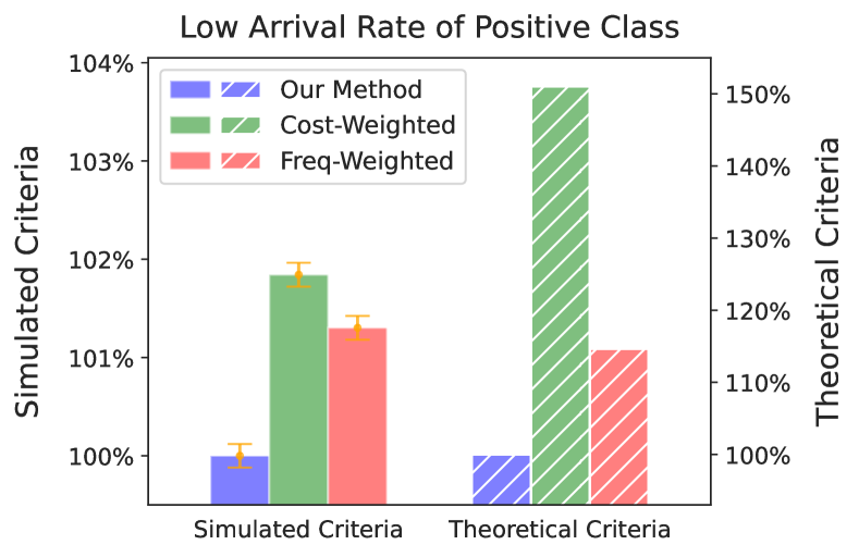
(b) model training

Figure 6: Our model selection approach vs. traditional weighted-accuracy-based methods. For thresholds or models optimized for each criteria, we present normalized simulated queueing cost (simulated critera) and relative regret in the heavy traffic limit (theoretical criteria). Our method reduces cumulative queueing costs; traditional methods exhibit varying rankings across settings.

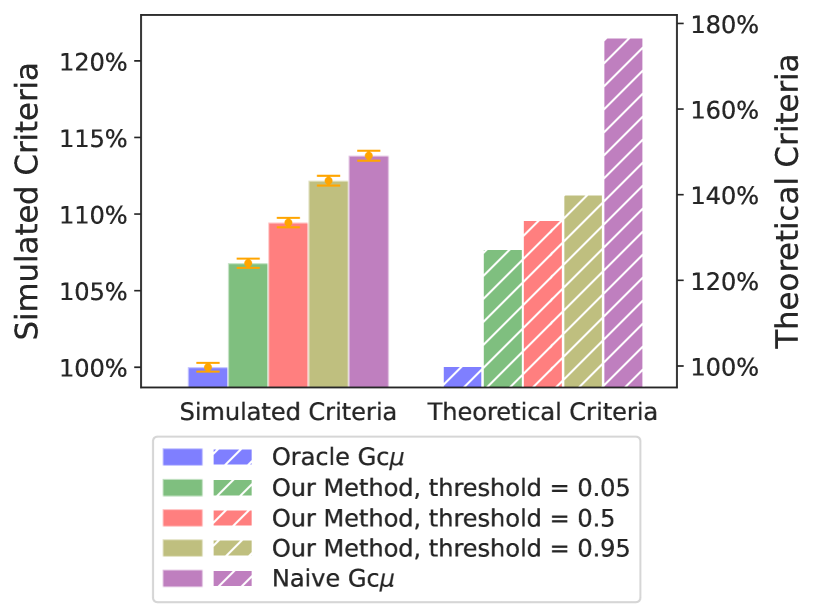
(a) Threshold selection

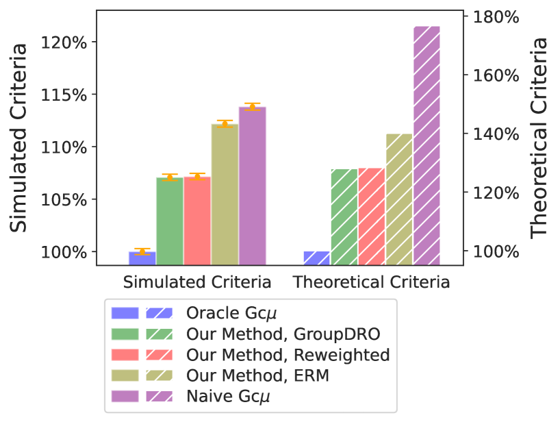
(b) Model selection

Figure 7: For different policies, we present our proposed model selection criteria (theoretical criteria) based on the relative regret $\tilde{J}(t;Q)/\tilde{J}^{*}(t;I)$ in the heavy traffic limit. To test its validity, we plot the simulated/acutal counterpart (simulated criteria) in the left. The relative ranking of policies based on our theoretical criteria exactly matches that given by the simulated quantities.

Comparison to Traditional Model Selection Criterias

Next, we explore the effectiveness of our model selection criterion by comparing it with traditional criteria that focus on predictive performance, such as accuracy, precision, recall, or their weighted combinations. In particular, we compare our evaluation metric $\tilde{J}^{*}(t;Q)/\tilde{J}^{*}(t;I)$ against two straightforward criteria: (i) cost-weighted accuracy, defined as $\frac{c_{1}q_{11}+c_{2}q_{22}}{c_{1}+c_{2}}$, and (ii) frequency-weighted accuracy, defined as $\frac{\lambda_{1}q_{11}+\lambda_{2}q_{22}}{\lambda_{1}+\lambda_{2}}$. As we observe below, model rankings under the traditional methods change across arrival rates, indicating their unreliability in queueing tasks.

We consider two different approaches for utilizing our metric: (i) setting the threshold for predicting the positive class for a fixed classifier, and (ii) model training. For threshold selection, we adopt the two environments from the above and generate covariates $X$ for positive and negative classes from independent normal distributions, $\mathcal{N}(0,0.5)$ and $\mathcal{N}(1,0.5)$, respectively. We focus on $f_{\theta}(X):=\mathbb{I}(X\geq\theta),~{}\forall~{}\theta\in[0,1]$, study thresholds selected by our method, cost-weighted accuracy, and frequency-weighted accuracy, and present corresponding simulated queueing cost under the P$c\mu$-rule in Figure 6 (a). (We use line search to to optimize each critera.) In Figure 6, we show the average simulated queueing costs (simulated criteria) at $T=1$ over $3\times 10^{6}$ independent sample paths using solid bars, with 2$\times$ the standard error encapsulated in the orange brackets. The shaded bar depicts the relative regret (theoretical criteria) corresponding to the selected thresholds in the heavy traffic limit. To facilitate comparison with our method, we normalize the theoretical and simulated criteria by the relative regret and the average simulated cumulative cost associated with our method, respectively.

We also study model training using relative regret. Specifically, we consider the 2 dimensional logistic regression problem, where covariates $\mathbf{X}\in\mathbb{R}^{2}$ for positive and negative classes are generated from $\mathcal{N}([1,0],[[1,-0.25],[-0.25,1]])$ and $\mathcal{N}([-1,0],[[1,0.75],[0.75,1]])$, respectively. For simplicity, we fix the threshold at 0.5 and focus on classifiers defined as: $f_{\mathbf{a},b}(\mathbf{X}):=\mathbb{I}([1+\exp\{-(\mathbf{a}^{\top}\mathbf{X}+b)\}]^{-1}\geq 0.5),~{}\forall~{}\mathbf{a}\in\mathbb{R}^{2},b\in\mathbb{R}.$ Due to the simplicity of the toy problem, we can directly minimize relative regret by grid search.

We compare our method with traditional methods using weighted cross-entropy loss as the training objective. Given weight $\mathbf{w}=[w_{1},w_{2}]$, predicted logits pred, and true labels $\mathbf{Y}$, the loss function is defined as $\ell_{w}(\mathbf{\texttt{pred}},\mathbf{Y}):=-\sum_{i:Y_{i}=1}w_{1}\log(\texttt{pred}_{i})-\sum_{j:Y_{j}=2}w_{2}\log(1-\texttt{pred}_{j})$. We study two straightforward methods: (i) cost-weighted loss, where $w_{1}=c_{1}/\lambda_{1},w_{2}=c_{2}/\lambda_{2}$, and (ii) frequency-weighted loss, where $w_{1}=1,w_{2}=1$. For both methods, we use the Adam optimizer with a learning rate of $0.1$, a batch size of 512, and train the model over $5$ epochs using $10^{5}$ datas points. We present the normalized theoretical and simulated criteria in Figure 6 (b).

As shown in Figure 6, in this simplified toy example, our method still outperforms traditional methods by $\sim 1-4\%$ in cumulative queueing costs. This demonstrates the effectiveness of our evaluation metric when queueing performance is the major concern. However, we note that there are discrepancies between the theoretical and simulated criteria in Figure 6 due to deviations from the heavy traffic limit. While we conduct a brute force grid search over classifier parameters in this simple setting, developing a practical and scalable training algorithm in more complex scenarios is an important direction of future work. As an interim solution, we can select between several candidate classifiers as we present next.

Numerical Experiments on CivilComments Dataset

To further understand the validity of our proposed model selection criteria, we revisit the fully general testing enviroment from Section 5. We study the performance of the P$c\mu$-rule, Oracle Gc$\mu$, and Naive G$c\mu$-rule, using the cumulative queueing cost at $T=1$ across $5\times 10^{4}$ independent sample paths. As the queueing cost of the Oracle Gc$\mu$-rule converges to $\tilde{J}^{*}(t;I)$, we normalize all simulated cumulative cost over each sample path by the average cumulative cost of the Oracle Gc$\mu$-rule. We refer to this quantity as “simulated” relative regret.

We demonstrate the utility of selecting and evaluating classifiers based on $\tilde{J}^{*}(t,Q)/\tilde{J}^{*}(t,I)$ using two tasks: (i) threshold selection for a fixed classifier, and (ii) model selection for a given collection of classifiers. In both cases, the ranking according to our proposed criteria aligns with simulated counterparts, illustrating how an analytic characterization of queueing cost can provide an effective comparison between ML models without extensive queueing simulation. For threshold selection, we consider the P$c\mu$-rule using the aforementioned ERM predictor and compare its queueing performance with thresholds being $[0.05,0.5,0.95]$, positioned from left to right in Figure 7 (a). In Figure 7, we present simulated relative regret using solid bars, with 2$\times$ the standard error encapsulated in the orange brackets. The shaded bar depicts our proposed model selection (theoretical criteria) given by the relative regret in the heavy traffic limit. For model selection, we consider the aforementioned three different classifiers: GroupDRO, Reweighted, and ERM with thresholds 0.05, 0.05, and 0.95. (These thresholds are chosen to showcase diverse queueing performances). In Figure 7 (b), we evaluate the P$c\mu$-rule using these models. We also compare P$c\mu$-rule to the Naive G$c\mu$-rule, where the classifier is fixed to the aforementeioned ERM classifier with threshold 0.5 in Figure 7 (a)(b).

We demonstrated that our proposed evaluation metric $\tilde{J}^{*}(t,Q)/\tilde{J}^{*}(t,I)$ effectively guides model selection by focusing on queueing performance. This approach ensures that the selected models optimize overall system performance, not just predictive accuracy, providing a robust basis for designing and selecting AI models in service systems.

7 Design of an AI-based triage system

Our characterization of queueing cost can be further utilized to design comprehensive job processing systems assisted by AI models. Motivated by content moderation systems on social media platforms [11, 64, 62], we study a triage system where an initial AI model filters out clear-cut cases, after which the queueing system serves remaining jobs (Figure 1). Standard triage systems in online platforms determine the filtering level using simple metrics such as maximizing recall subject to a fixed high precision level (e.g., [11]). These designs [2, 54, 67, 1] lead to suboptimal system performance as they do not consider the downstream operational cost such as hiring cost of human reviewers and queueing costs.

In this section, we provide a novel framework for designing AI-assisted triage systems that jointly optimize the filtering and queueing systems, taking into account all four types of costs: filtering costs, hiring costs, misclassification costs, and queueing congestion costs. Our objective can be easily estimated using a small set of validation data and a simple simulation of a (reflected) Brownian motion, allowing us to find the optimal filtering level through methods like line search. In Section 7.4, we conduct numerical experiments to demonstrate effectiveness of this approach. We find that prediction-based metrics, which is a norm in practice, may align with the total cost when either filtering cost or hiring cost dominates, but it fails to do so in more complicated settings with trade-offs between different types of costs. Our method avoids computationally expensive queueing simulations, and consistently identifies the optimal filtering and staffing levels in all of these scenarios by simply simulating a (reflected) Brownian motion.

7.1 Model of the AI-based triage system

We consider a sequence of single-stream incoming jobs that arrive at the triage system. We assume the $n$th system operates on a finite time horizon $[0,n]$, starts empty, has i.i.d. interarrival times with an arrival rate of $\Lambda^{n}$. With a slight abuse of notation, we let $u^{n}_{i}$ be the interarrival time of the $i$th job in system $n$, $U^{n}_{0}(t)$ be the arrival time of the $\lfloor t\rfloor$th job in system $n$, and $A^{n}_{0}(t)$ be the total number of jobs arriving in the triage system $n$ up to time $t$. For simplicity, we consider a two-class setting, with class 1 representing toxic content and class 2 representing non-toxic content. For each job, a tuple of (observed features, true class label, service time), denoted as $(X^{n}_{i},Y^{n}_{i},v^{n}_{i})$, is generated identically and indepedently of its arrival time $u^{n}_{i}$. Similar to our model in Section 2, $v^{n}_{i}$ and $X^{n}_{i}$ are conditionally independent given $Y^{n}_{i}$.

We use the binary classifier $f_{\theta}$ for the filtering procedure across all systems $n$. With a slight abuse of notation, let $f_{\theta}(\cdot)\in[0,1]$ now be the toxicity score instead of the predicted class label. Specifically, the classifier outputs $f_{\theta}(X^{n}_{i})\in[0,1]$ based on the observed features $X^{n}_{i}$ for each job $i$. The system designer is tasked with choosing a threshold $z_{\text{FL}}$ that affects the (triage) filtering level: an arriving job in system $n$ can pass the filtering system and enter the queueing system if and only if $f_{\theta}(X^{n}_{i})\geq z_{\text{FL}}$. Content that are filtered out are not reviewed and can remain on the platform. A higher filtering level $z_{\text{FL}}$ filters more jobs out, resulting in higher false negative rate (more filtering and misclassification costs), fewer human reviewers required (lower hiring cost), and a complex effect on the downstream queueing cost.

Each job that passes the filtering system is subsequently sent to human reviewers (queueing system). Given the filtering level $z_{\text{FL}}$, we use the same number of reviewers $\Gamma(z_{\text{FL}})$ across all systems, where $\Gamma(z_{\text{FL}})$ is a predetermined decision variable, fixed in advance and not subject to randomness. We assume that for each system $n$, all reviewers have the same service rate for class $k$ jobs, i.e., $\mu_{k,r}^{n}=\mu_{k}^{n},~{}\forall~{}k\in\{1,2\}$ for each reviewer $r\in[\Gamma(z_{\text{FL}})]$. To ensure workload equality and fairness among reviewers, we assume jobs passing through the filtering system are assigned to one and only one human reviewer with equal probability $1/\Gamma(z_{\text{FL}}),$ independently of any other random objects. Each human reviewer operates their own single-server queueing system. The jobs allocated to the $r$th reviewer corresponds to their arrival processes, denoted as $A_{\text{ps},r}^{n}(t)$, which are splited from the common arrival process after filtering, denoted as $A_{\text{ps},0}^{n}(t)$. For the $j$th job passing through the filtering system, let $\mathbf{B}^{n}_{j}:=(B_{j1}^{n},\ldots,B_{j\Gamma(z_{\text{FL}})}^{n})$ be the one-hot encoded representation of the reviewer it is assigned to. Then, $A_{\text{ps},r}^{n}(t):=\sum_{j=1}^{A_{\text{ps},0}^{n}(t)}B_{jr},~{}\forall~{}t\in[0,n],r\in[\Gamma(z_{\text{FL}})]$.

For simplicity, we assume all reviewers utilize $f_{\theta}$ to predict the class labels of incoming jobs. The system designer must decide another threshold $z_{\text{TX}}\geq z_{\text{FL}}$ that affects the toxicity classification. In particular, for the $s$th job assigned to reviewer $r$, it is predicted to be toxic (class 1), i.e., $\underline{Y}^{n}_{s1,r}=1$, if and only if $f_{\theta}(X^{n}_{s,r})\geq z_{\text{TX}}$. We assume all human reviewers adopt the same scheduling policy. Similar to our model in Section 2, reviewers use the predicted class $\underline{\mathbf{Y}}^{n}_{s,r}$ and feasible scheduling policies must satisfy a variant of Definition 1.

Throughout this section, we use $i$ when counting jobs that arrive at the triage system; $j$ for jobs that pass the filtering system and arrive at the queueing system; $s$ for jobs assigned to a human reviewer; and $r$ for human reviewers (servers). For a stochastic process $A_{\text{ps},0}^{n}(t)$, the subscript ps indicates processes associated with jobs passing through the filter and arriving at the queueing system. We use the subscript $0$ to indicate the total arrival process and $r$ to indicate processes associated with the reviewer $r$. We denote our decision variables $(z_{\text{FL}},z_{\text{TX}})$ by $\mathbf{z}$. We summarize our assumptions for the AI-based triage system below.

Assumption F (Data generating processes for the AI-based triage system).

For any system $n\in\mathbb{N}$, (i) $\{(u_{i}^{n},v_{i}^{n},X_{i}^{n},Y_{i}^{n}):i\in\mathbb{N}\}$ is a sequence of i.i.d. random vectors; (ii) $\{u_{i}^{n}:i\in\mathbb{N}\}$ and $\{(v_{i}^{n},X_{i}^{n},Y_{i}^{n}):i\in\mathbb{N}\}$ are independent; (iii) for any $i\in\mathbb{N}$, $v^{n}_{i}$ and $X^{n}_{i}$ are conditionally independent given $Y^{n}_{i}$; (iv) $\{\mathbf{B}^{n}_{j}:j\in\mathbb{N}\}$ is a sequence of i.i.d. random vectors; (v) $\{\mathbf{B}^{n}_{j}:j\in\mathbb{N}\}$ is independent of $\{u_{i}^{n}:i\in\mathbb{N}\}$ and $\{(v_{i}^{n},X_{i}^{n},Y_{i}^{n}):i\in\mathbb{N}\}$.

The data generating process for the AI-based triage system is crucial to our analysis, because it enables the reduction of the scheduling problem for all reviewers to stochastically identical single-server scheduling problems across the reviewers. Assumption F (i), (iv) and (v) ensure that each reviewer $r$ has a single stream of jobs with i.i.d. tuples $\{(v^{n}_{s,r},X^{n}_{s,r},Y^{n}_{s,r}):s\in\mathbb{N}\}$. More importantly, the tuples associated with reviewer $r$ become independent of those of any other reviewers. This leads to the joint convergence of the diffusion-scaled processes defined by $\{(v^{n}_{s,r},X^{n}_{s,r},Y^{n}_{s,r}):s\in\mathbb{N}\}$ across all reviewers $r\in[\Gamma(z_{\text{FL}})]$. In addition, similar to Section 2, Assumption F (i), (iv), and (v) allow us to disentangle the interarrival times $\{u^{n}_{s,r}:s\in\mathbb{N}\}$ from the filtering process, service processes, and the covariates, ensuring the joint convergence of the diffusion-scaled processes defined by $\{u^{n}_{s,r}:s\in\mathbb{N}\}$ across the reviewers $r\in[\Gamma(z_{\text{FL}})]$. Since Assumption F (ii) and (v) imply independence between $\{(v^{n}_{s,r},X^{n}_{s,r},Y^{n}_{s,r}):s\in\mathbb{N}\}_{r\in[\Gamma(z_{\text{FL}})]}$ and $\{u^{n}_{s,r}:s\in\mathbb{N}\}_{r\in[\Gamma(z_{\text{FL}})]}$, we can derive the desired joint convergence (Lemma 30) and apply our sample path analysis at the reviewer level. For further discussion, see Appendix G.1.

7.2 Heavy traffic conditions for the AI-based triage system

In the sequel, we assume the triage system operates under heavy traffic conditions and analyze the limiting system. Denote the conditional probability of a class $k$ job passing through the level $z$ as $g_{k}^{n}(z):=\mathbb{P}^{n}[f_{\theta}(X_{i}^{n})\geq z\mid Y_{ik}^{n}=1],~{}\forall~{}z\in[0,1],~{}k\in\{1,2\}$. Similar to Assumption B, we adopt the following heavy traffic conditions for the AI-based triage system.

Assumption G (Heavy traffic conditions for AI-based triage system).

Given a classifier $f_{\theta}$ and a sequence of triage systems, we assume that there exist $\Lambda$, $\mu_{k}$, and $g_{k}:[0,1]\rightarrow[0,1]$ such that (i) for any filtering level $z_{\text{FL}}\in[0,1]$ and class $k\in\{1,2\}$, we have that

$$n^{1/2}(\Lambda^{n}-\Lambda)\rightarrow 0,\quad n^{1/2}(\mu_{k}^{n}-\mu_{k})\rightarrow 0,\quad n^{1/2}(g_{k}^{n}(z_{\text{FL}})-g_{k}(z_{\text{FL}}))\rightarrow 0;$$

(ii) given the filtering level $z_{\text{FL}}$, the number of hired reviewers satisfies $\Gamma(z_{\text{FL}})=\Lambda\sum_{k=1}^{2}\frac{p_{k}g_{k}(z_{\text{FL}})}{\mu_{k}}.$

We adopt Assumption G to ensure that each reviewer aligns with Assumption B. Specifically, according to Assumption G (i) and [68, Theorem 9.5.1], we can show that for each reviewer $r$, their class prevalence $p^{n}_{k,r}(z_{\text{FL}}):=\mathbb{P}^{n}[Y_{sk,r}^{n}=1\mid f_{\theta}(X^{n}_{s,r})\geq z_{\text{FL}}]$ and confusion matrix $\underline{q}^{n}_{kl,r}(\mathbf{z}):=\mathbb{P}^{n}[\underline{Y}^{n}_{sl,r}=1\mid f_{\theta}(X^{n}_{s,r})\geq z_{\text{FL}},Y_{sk,r}^{n}=1]$ all converge to their limits $p_{k}(z_{\text{FL}})$ and $\underline{q}_{kl}(\mathbf{z})$ at the rate of $o(n^{-1/2})$ (Lemma 32). We use $Q^{n}(\mathbf{z})$ and $Q(\mathbf{z})$ to denote the prelimit and limiting confusion matrix for each reviewer. In addition, by Assumption G (ii), we have that

$$n^{1/2}\Big{[}\frac{\Lambda^{n}}{\Gamma(z_{\text{FL}})}\sum\limits_{k=1}^{2}\frac{p_{k}^{n}g_{k}^{n}(z_{\text{FL}})}{\mu_{k}^{n}}-1\Big{]}\rightarrow 0,$$ (7.1)

which indicates that each reviewer operates under heavy traffic conditions and matches (2.2). According to Assumption G (ii), when all reviewers operates under heavy traffic conditions, the number of reviewers is solely determined by limiting traffic indensity and the filtering level $z_{\text{FL}}$. Thus, our decision variables are filtering level $z_{\text{FL}}$ and toxicity level $z_{\text{TX}}$, with the number of reviewers determined accordingly. Intuitively, as the filtering level $z_{\text{FL}}$ increases, the traffic intensity decreases and the number of reviewers hired also decreases.

Starting from Assumptions F and G, we first establish the joint convergence result in Lemma 30. As Assumptions F and G are compatible with Assumptions A and B, we derive a common probability space $\mathbb{P}_{\text{copy}}$ in Lemma 31 and apply the previous results on single-server queueing systems to each reviewer. This allows us to establish the limiting total cost of the triage system in Section 7.3.

7.3 Total Cost of the AI-based triage system

Motivated by content moderation problems, we divide the total cost into four components: filtering cost, hiring cost, misclassification cost, and queueing cost. Since the P$c\mu$-rule is optimal for each single-server queueing system under heavy traffic conditions, we can explicitly quantify the best possible queueing cost of the limiting system under quadratic cost assumption (Assumption E). This enables us to determine the limiting total cost and minimize it to find the optimal filtering and classification levels $(z_{\text{FL}},z_{\text{TX}})$ for a fixed classifier $f_{\theta}$. In the following, we first define each cost component and then establish the limiting total cost in Theorem 5.

Definition 4 (Total cost of the AI-based triage system).

Given a classifier $f_{\theta}$, filtering level $z_{\text{FL}}$, toxicity level $z_{\text{TX}}$, the number of hired reviewers $\Gamma(z_{\text{FL}})$, and a sequence of AI-based triage system, for a sequence of feasible policies $\{\text{$\pi_{n}$}\}$, define the cost incurred as the following.

1. (Filtering cost) For each job that is filtered out, the unit costs for toxic and non-toxic jobs are $c_{\text{FL},1}>0$ and $c_{\text{FL},2}<0$. The total filtering cost up to time $t\in[0,n]$ is

   $$G^{n}(t;z_{\text{FL}}):=c_{\text{FL},1}\sum_{i=1}^{A_{0}^{n}(t)}\mathbb{I}(f_{\theta}(X^{n}_{i})<z_{\text{FL}})\cdot Y^{n}_{i1}+c_{\text{FL},2}\sum_{i=1}^{A_{0}^{n}(t)}\mathbb{I}(f_{\theta}(X^{n}_{i})<z_{\text{FL}})\cdot Y^{n}_{i2},$$

   and $\tilde{G}^{n}(t;z_{\text{FL}}):=n^{-1}G^{n}(nt;z_{\text{FL}})$ is the scaled filtering cost.

2. (Hiring Cost) Each reviewer costs $c_{r}>0$ per unit of time.

3. (Misclassification Cost) The per-job cost of false positive, false negative, true positive, or true negative are $c_{\text{fp}},c_{\text{fn}},c_{\text{tp}},c_{\text{tn}}$, respectively. The total misclassification cost up to time $t$ is $M^{n}(\mathbf{z},t)$, and its scaled counterpart is $\tilde{M}^{n}(t;\mathbf{z}):=n^{-1}M^{n}(nt;\mathbf{z})$.

4. (Queueing Cost) For each system $n$ and reviewer $r$, $J^{n}_{\text{$\pi_{n}$},r}(t;Q^{n}(\mathbf{z}))$ is the cumulative queueing cost as defined in Section 3.1, and $\tilde{J}^{n}_{\text{$\pi_{n}$},r}(t;Q^{n}(\mathbf{z})):=n^{-1}J^{n}_{\text{$\pi_{n}$},r}(nt;Q^{n}(\mathbf{z}))$ is its scaled counterpart.

The total cost incurred up to time $t$ is defined by

$$F_{\text{$\pi_{n}$}}^{n}(t;\mathbf{z})=\underbrace{G^{n}(t;z_{\text{FL}})}_{\text{filtering}}+\underbrace{c_{r}\Gamma(z_{\text{FL}})t}_{\text{hiring}}+\underbrace{M^{n}(t;\mathbf{z})}_{\text{misclassification}}+\underbrace{\sum_{r=1}^{\Gamma(z_{\text{FL}})}J^{n}_{\text{$\pi_{n}$},r}(t;Q^{n}(\mathbf{z}))}_{\text{queueing}},~{}\forall~{}t\in[0,n],$$

and $\tilde{F}_{\text{$\pi_{n}$}}^{n}(t;\mathbf{z}):=n^{-1}F_{\text{$\pi_{n}$}}^{n}(nt;\mathbf{z})$ is its scaled counterpart.

For any filtering level $z_{\text{FL}}$ and toxicity level $z_{\text{TX}}$, we can easily establish the optimal total cost of the AI-based triage system under heavy traffic limits by extending Proposition 6, Theorem 3, and Proposition 4. Such optimal cost can be achieved by applying the P$c\mu$-rule to all reviewers as shown in (7.2).

Theorem 5 (Total cost the AI-based triage system).

Given a classifier $f_{\theta}$, filtering level $z_{\text{FL}}$, toxicity level $z_{\text{TX}}$, the number of hired reviewers $\Gamma(z_{\text{FL}})$, and a sequence of AI-based triage system, suppose that Assumptions E, F, G, and H hold. There exists a common probability space $\mathbb{P}_{\text{copy}}$ such that

1. (Lower bound) under any feasible policies $\{\text{$\pi_{n}$}\}$, the associated total cost $\tilde{F}_{\text{$\pi_{n}$}}^{n}(t;\mathbf{z})$ satisfies $\liminf\limits_{n}\tilde{F}_{\text{$\pi_{n}$}}^{n}(t;\mathbf{z})\geq\tilde{F}^{*}(t;\mathbf{z})$, $\forall~{}t\in[0,1]~{}\mathbb{P}_{\text{copy}}-a.s.$. For the original processes under $\mathbb{P}^{n}$, under any feasible policies $\{\pi^{\prime}_{n}\}$,

   $$\liminf\limits_{n}\mathbb{P}^{n}[\tilde{F}_{\pi^{\prime}_{n}}^{n}(t;\mathbf{z})>x]\geq\mathbb{P}_{\text{copy}}[\tilde{F}^{*}(t;\mathbf{z})>x],~{}\forall x\in\mathbb{R},t\in[0,1];$$

2. (Optimality) under the P$c\mu$-rule, we have that $\tilde{F}^{n}_{\text{Pc$\mu$}}(\cdot;\mathbf{z})\rightarrow\tilde{F}^{*}(\cdot;\mathbf{z})$ $\text{in }(\mathcal{D},\|\cdot\|),~{}\mathbb{P}_{\text{copy}}-a.s.$. For the original processes under $\mathbb{P}^{n}$, $\tilde{F}^{n}_{\text{Pc$\mu$}}(\cdot;\mathbf{z})\Rightarrow\tilde{F}^{*}(\cdot;\mathbf{z})$ $\text{in }(\mathcal{D},J_{1})$, and in particular, $\mathbb{P}^{n}[\tilde{F}^{n}_{\text{Pc$\mu$}}(t;\mathbf{z})>x]\rightarrow\mathbb{P}_{\text{copy}}[\tilde{F}^{*}(t;\mathbf{z})>x],~{}\forall~{}x\in\mathbb{R},t\in[0,1]$.

Here, the optimal total cost $\tilde{F}^{*}(t;\mathbf{z})$ is defined as

$$\tilde{F}^{*}(t;\mathbf{z}):=\tilde{G}^{*}(t;z_{\text{FL}})+c_{r}\Gamma(z_{\text{FL}})t+\tilde{M}^{*}(t;\mathbf{z})+\sum_{r=1}^{\Gamma(z_{\text{FL}})}\tilde{J}_{r}^{*}(t;Q(\mathbf{z})),$$ (7.2)

where

$$\tilde{G}^{*}(t;z_{\text{FL}})=\Lambda t\cdot[c_{\text{FL},1}p_{1}(1-g_{1}(z_{\text{FL}}))+c_{\text{FL},2}p_{2}(1-g_{2}(z_{\text{FL}}))],$$

$$\tilde{M}^{*}(t;\mathbf{z})=\Lambda t\cdot\big{[}p_{1}g_{1}(z_{\text{FL}})[c_{\text{tp}}\underline{q}_{11}(\mathbf{z})+c_{\text{fn}}\underline{q}_{12}(\mathbf{z})]+p_{2}g_{2}(z_{\text{FL}})[c_{\text{fp}}\underline{q}_{21}(\mathbf{z})+c_{\text{tn}}\underline{q}_{22}(\mathbf{z})]\big{]}$$

$$\tilde{J}_{r}^{*}(t;Q(\mathbf{z}))=\frac{\beta_{1}(Q(\mathbf{z}))\beta_{2}(Q(\mathbf{z}))}{2\big{[}\beta_{1}(Q(\mathbf{z}))+\beta_{2}(Q(\mathbf{z}))\big{]}}\int_{0}^{t}\tilde{W}_{+}(s;\mathbf{z},r)^{2}\mathrm{d}s,$$

for all $t\in[0,1]$, and $\tilde{W}_{+}(t;\mathbf{z},r)$ is the limiting remaining total workload process of reviewer $r$ as defined in Lemma 33.

According to Theorem 5, we can minimize (7.2) to find the optimal filtering and toxicity levels $(z_{\text{FL}},z_{\text{TX}})$ for a given classifier $f_{\theta}$. In particular, (7.2) depends solely on limiting exogenous quantities such as $\Lambda$, $p_{k}(z_{\text{FL}})$, $\underline{q}_{kl}(z_{\text{FL}})$ that can be easily estimated given a small set of validation data. $\tilde{W}_{+}^{n}(t;\mathbf{z},r)$ is a reflected Brownian motion with a known drift and covariance (see further discussion in Appendix G.3), so we can estimate the total cost using a simulated (reflected) Brownian motion. The optimal level $\mathbf{z}^{*}$ can be then found through a simple line search over $[0,1]$. Our approach avoids traditional queueing simulations, which can be costly and time-consuming, making it practical and scalable for real-world applications.

7.4 Numerical Experiments for the AI-based triage system

Our formulation trades off multiple desiderata, in contrast to the standard industry practice that choose $\mathbf{z}$ solely based on prediction metrics, such as maximizing recall subject to a fixed high precision level [11]. To compare our proposed approach with such standard triage design approaches, we consider the 2-class content moderation problem described in Section 6. We assume the covariates for positive and negative classes are generated in the same fasion as in the 2d logistic regression problem in Section 6, and consider the logistic regression classifier $f_{\theta}$ developed by minimizing the equally-weighted cross-entropy loss ($w_{1}=1$, $w_{2}=1$). For simplicity, we fix the toxicity level $z_{\text{TX}}=0.5$ and only study how filtering level $z_{\text{FL}}$ affects the total cost.

We examine the setting where the positive class has a relatively high arrival rate to mimic the setting where only flagged content is sent to the triage system, which results in a relatively high proportion of positive class; recall Figure 1. In particular, we set $[\Lambda_{1},\Lambda_{2}]=[10000,40000]$, $[\mu_{1},\mu_{2}]=[50,200]$, where $[\Lambda_{1},\Lambda_{2}]$ is the arrival rate of positive and negative classes to the triage system, and $[\mu_{1},\mu_{2}]$ is the common service rate for the positive and negative classes across all reviewers. We consider three cases: (i) filtering costs dominate, (ii) hiring costs dominate, and (iii) a trade-off between filtering cost and hiring costs. The filtering costs and hiring costs are set as follows: (i) $[c_{\text{FL},1},c_{\text{FL},2}]=[200,-3]$, $c_{r}=500$, (ii) $[c_{\text{FL},1},c_{\text{FL},2}]=[20,-3]$, $c_{r}=5000$, and (iii) $[c_{\text{FL},1},c_{\text{FL},2}]=[20,-3]$, $c_{r}=500$. In all cases, the misclassification costs are set as $[c_{\text{fp}},c_{\text{fn}},c_{\text{tp}},c_{\text{tn}}]=[3,3,-3,-3]$, and the delay costs are set as $C_{\cdot}(t)=c_{\cdot}t^{2}/2$ with $c_{1}=15,c_{2}=1$.

Our goal is to find the best filtering level $z_{\text{FL}}$ that minimizes the total cost. We compare our method that minimizes (7.2) to the following classical method from Chandak [11], which finds the filtering level $z_{\text{FL}}$ by maximizing recall subject to a high precision level lower bound $z_{\text{prec}}\in[0,1]$. Both methods can be effectively implemented using small set of validation data and a linear search. We set the search range for $z_{\text{FL}}$ as $[0.05,0.48]$.

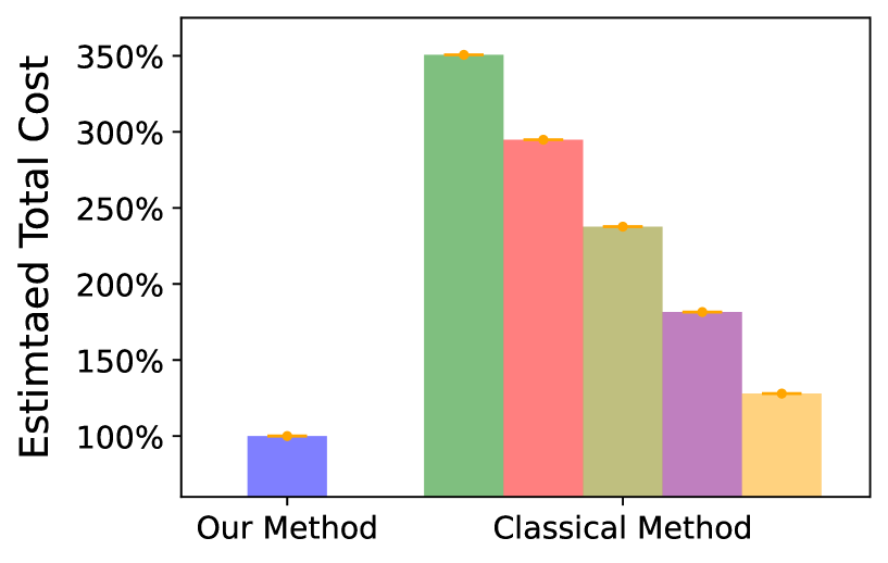
(i) Filtering costs dominate

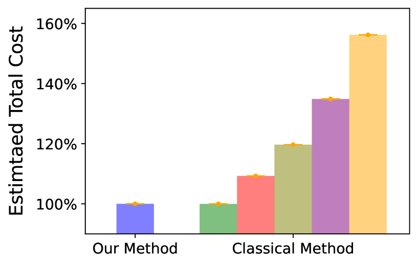
(ii) Hiring costs dominate

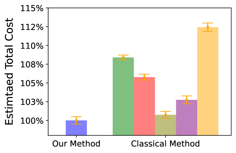
(iii) Trade-off between

filtering and hiring costs

Figure 8: For different methods, we consider the selected filtering level $z_{\text{FL}}$ and present the associated estimated total cost of the AI-based triage system. The classical method maximizes recall subject to the precision level $[0.93,0.94,0.95,0.96,0.97]$, positioned from left to right. This method exhibits highly varying total cost even at high precision levels, making it hard to determine the best filtering level. In contrast, our method effectively minimizes the total cost by cheap simulations of (reflected) Brownian motion.

In Figure 8, we present the average total cost over 10K sample paths of the simulated (reflected) Brownian motion, with $2\times$ the standard error encapsulated in the orange brackets. For the classical method, we set the precision level as $[0.93,0.94,0.95,0.96,0.97]$, positioned from left to right. To facilitate comparison with our method, we normalize the estimated total cost by that of our method. We observe that the classical method exhibits highly varying total cost (by $\sim 10\%-250\%$) even at high precision levels in Figure 8. This demonstrates the importance of selecting the right filtering level to minimize the total cost. In addition, for the classical method, it also shows the total cost is highly sensitive to the precision level. Therefore, the precision level serves as an important hyperparameter, and it is challenging to determine the best precision level that corresponds to optimal filtering level using the classical method.

Such challenge arises since our method takes a holistic view of the entire triage system, yet the classical method only considers the prediction metrics. In our toy example, a higher precision level leads to a lower selected filtering level $z_{\text{FL}}$, which results in lower filtering costs and higher hiring costs. Figure 8 (i)(ii) corresponds to simpler settings where the total cost aligns with prediction metrics. That is, when filtering costs or hiring costs dominate, the total cost is monotone with respect to the filtering level and thus the precision level, as shown in Figure 8 (i)(ii). Therefore, when adopting the classical method, we can simply choose the precision level at the search boundary, which yields a filtering level near the search boundary that minimizes the total cost. In contrast, in Figure 8 (iii), where there is a trade-off between filtering and hiring costs, the total cost is non-monotone and “U”-shaped with respect to the precision/filtering level. In this case, prediction metrics fails to capture the total cost. While hyperparameter (precision) tuning based on total costs is possible, the classical method merely shifts our search space to hyperparameters (precision levels). In other words, hyperparameter tuning is equivalently to a naive line search for the decision variable (filtering level $z_{\text{FL}}$) based on simulated total cost and the classical method does not serve as effective objectives/metrics. More importantly, without our Theorem 5, the total cost can only be estimtaed through multiple costly simulations of the entire triage system. Our method, in contrast, effectively identifies the correct objective and finds the best filtering level through cheap simulations of (reflected) Brownian motion.

Our numerical experiments demonstrate the the effectiveness of our method and the importance of taking a holistic view of the entire content moderation system. We hope our method paves the way for more advanced system designs for complex AI-based triage systems in practical use.

8 Discussion

Our work builds on the large literature on queueing, as well as the more nascent study of decision-making problems with prediction models [4, 41, 57, 33, 12, 60]. Unlike previous works that study relatively simple optimization problems (e.g., linear programming [19]) that take as input predictions, our scheduling setting requires modeling the endogenous impact of misclassifications.

8.1 Related work

Heavy traffic analysis allows circumventing the complexity of state/policy spaces via state-space collapse, thereby identifying asymptotically optimal queueing decisions [28, 40, 50, 63, 68]. The $c\mu$-rule was shown to be optimal among priority rules in [15], and Van Mieghem [63] proved heavy traffic optimality of the G$c\mu$-rule with convex delay costs in single-server systems with general distributions of interarrival and service times. Under a heavy traffic regime defined with a complete resource pooling condition [27], Mandelbaum and Stolyar [40] extended the result to multi-server and multi-class queues. In the many server Halfin-Whitt heavy traffic regime (where the server pool is also scaled [26]), Gurvich and Whitt [25] showed their state-dependent policy that minimizes the holding cost reduces to a simple index-rule with linear holding costs, and to the G$c\mu$-rule with convex costs. When customers in queues can abandon systems, a similar index rule that accounts for the customer abandonment rate was shown to minimize the long-run average holding cost under the many-server fluid limit [5].

We focus on the single-server model and relax a common assumption that the class of every job is known. We study the impact of AI models in queueing jobs, and use the heavy traffic limit to analyze the downstream impacts of miclassifications. Our results provide a unified framework for evaluating and selecting AI models for optimal queueing. Along the way, we also provide rigorous proofs for the classical setting with known classes by proving unjustified steps in Van Mieghem [63] and qualifying conditions under which they hold.

The challenge of unknown traffic parameters was identified as early as Cox [14]. Using an off-policy ML model in queueing systems was also proposed for classifying jobs into different types or priority classes [57, 60] and predicting service times [12]. Argon and Ziya [4], Singh et al. [57] focus on minimizing the mean stationary waiting time with Poisson arrivals, while we allow general distributions of arrival and service times in our heavy traffic analysis. Although Argon and Ziya [4, Section 8] proposes a policy similar in form to the P$c\mu$-rule, their policy is compared to the FCFS policies in terms of the stationary waiting time, while our analysis shows the optimality of P$c\mu$-rule over all feasible policies in terms of cumulative cost. Sun et al. [60] consider a two-class setting (triage or not) where classes can be inferred with additional time, and analyze when it is optimal to triage all (or no) jobs. Importantly, they assume service times follow predicted classes.  Chen and Dong [12] develop a two-class priority rule using predicted service times and show the convergence of the queue length process to the same limit as in the perfect information case when estimation error is sufficiently small. In contrast, we characterize the optimal queueing cost given a fixed classifier instead of aiming to match the performance of the perfect classifier. Our approach allows us to provide guidance on model selection for classifiers as we illustrate in Section 6.

Going beyond simple index policies, deep reinforcement learning (DRL) algorithms can be used for queueing systems with unknown parameters. Dai and Gluzman [16] develop a policy optimization approach for multiclass Markovian queueing networks and proposes several variance reduction techniques. Pavse et al. [47] combine proximal and trust region-based policy optimization algorithms [55] with a Lyapunov-inspired technique to ensure stability. Developing further approaches to overcome the challenges of applying RL algorithms in queueing (e.g., infinite state spaces, unbounded costs) is a fertile direction of future research.

There is a growing body of work on learning in queueing systems that focus on online learning and analyze regret, the performance gap between the learning algorithm and the best policy in hindsight with the complete knowledge of system parameters [16, 21, 22, 23, 34, 35, 36, 56, 65, 66, 70]. Inspired by the well-known static priority policies in queueing literature [5, 6, 40, 48, 49, 63], empirical versions of such policies were proposed where plug-in estimates of unknown parameters are used to compute static priorities. When service rates are unknown, Krishnasamy et al. [35] propose an empirical $c\mu$ rule for multi-server settings and show constant regret for linear cost functions, and Zhong et al. [70] develop an algorithm for learning service and abandonment rates in time-varying multiclass queues with many servers and show the empirical $c\mu/\theta$ rule achieves optimal regret. In the machine scheduling literature, where a finite set of jobs are given (with no external arrivals), Lee and Vojnovic [37] studies settings where delay costs are unknown, and show that a plug-in version of the $c\mu$-rule can achieve near-optimal regret when coupled with an exploration strategy.

For more general queueing networks, Walton and Xu [66] present a connection between the MaxWeight policy [61] and Blackwell approachability [9], relating the waiting time regret to that of a policy for learning service rates. Borrowing insights from the stochastic multi-armed bandit literature [58], a body of work [13, 34, 36, 59, 65] develops learning algorithms to minimize expected queue length, addressing challenges in the queueing bandit model such as ensuring stability until the parameters are sufficiently learned [36]. Freund et al. [22] propose a new performance measure of time-averaged queue length, and show near-optimality of the upper-confidence bound (UCB) algorithm in a single-queue multi-server setting, as well as new UCB-type variants of MaxWeight and BackPressure [61] in multi-queue systems and queueing networks, respectively. For queueing systems with multi-server multiclass jobs, Yang et al. [69] recently developed another UCB-type variant of the MaxWeight algorithm. Learning service rates has also been studied in decentralized queueing systems, where classes of jobs are considered as strategic agents [21, 23, 56] and stability is a primary concern. Motivated by content moderation, a concurrent work [38] studies the joint decision of content classification, and admission and scheduling for human review in an online learning framework.

8.2 Future directions

We discuss limitations of our framework and pose future directions of research. First, implementing the P$c\mu$-rule needs more information than the previous index-based policies. It necessitates arrival information, $\lambda$ and $\{p_{k}\}_{k\in[K]}$, as well as the misclassification probabilities $Q^{n}=(\underline{q}_{kl}^{n})_{k,l\in[K]}$. In practice, such parameters need to be estimated on a limited amount of data and estimation errors are unavoidable.

Extension of the queueing model

We identify conceptual and analytical challenges in extending our framework to the multiserver setting. Modeling the extension after Mandelbaum and Stolyar [40] who consider known true classes, we can posit the complete resource pooling (CRP) condition. This condition requires the limit of the arrival rates to be located in the outer face of the stability region, and to be uniquely represented as a maximal allocation of the servers’ service capacity. For our setting in Section 2, the main challenge is that the CRP condition will not necessarily hold on the arrival and service rates of the predicted classes. Because the service rate of each predicted class in prelimit will be a mixture of the original service rates as $\underline{\mu}_{l}^{n}$ in Definition 10, the CRP condition on true classes may not be preserved for predicted classes.

Understanding of how prediction error interacts with queueing performance under general dynamics is an important direction of future research. For example, when jobs exhibit abandonment behavior, a suitable adjustment to the c$\mu$-rule minimizes the long-run holding cost under many-server fluid scaling [5]. Policies that simultaneously account for predictive error and job impatience may yield fruit.

Design of queueing systems under class uncertainty

While we focus on optimal scheduling, an even more important operational lever is the design of the queueing system [20, 30]. For example, designing priority classes that account for predictive error is a promising research direction [12]. In our model, if we keep the limiting distributions of the interarrival and service times the same, class designs satisfying the heavy traffic condition (2.2) should have an identical limiting total workload $\tilde{W}_{+}$ by Proposition 1, implying similar forms of the lower bound in (3.3). Given this observation, we may investigate how class design interacts with the AI model’s predictive performance.

Combining the P$c\mu$-rule with AI-based approaches

The performance of RL algorithms degrade under distribution shift, and simple index-based policies may offer robustness benefits. The two approaches may provide synergies. For example, we can pre-train a policy to initially imitate an index-based policy, and then fine-tune it to maximize performance in specific environments.

For quadratic costs, we showed the effectiveness of using the relative regret $\tilde{J}^{*}(\cdot;Q)$ to select the classification threshold. Alternatively, we could directly fine-tune the classifier to minimize this metric, which may further enhance downstream queueing performance, albeit at the cost of increased engineering complexity.

Appendices

Appendix A Diffusion limits

We consider the following processes: partial sum process of interarrival time $U_{0}^{n}(t)$ that depends solely on $\{u_{i}^{n}:i\in\mathbb{N}\}$, partial sum process of service time $V_{0}^{n}$ and two other processes $\underline{\mathbf{Z}}^{n}:=(\underline{Z}_{kl}^{n})_{k,l\in[K]},\underline{\mathbf{R}}^{n}:=(\underline{R}^{n}_{l})_{l\in[K]}$ that solely relies on $\{(X_{i}^{n},Y_{i}^{n},v_{i}^{n}):i\in\mathbb{N}\}$. In particular, given system $n$, $\underline{Z}_{kl}^{n}(t)$ is the total number of jobs from real class $k$ and predicted as class $l$ and $\underline{R}_{l}^{n}(t)$ is the total service time requested by jobs predicted as class $l$, among the first $\lfloor t\rfloor$ jobs arriving in the system:

$$\underline{Z}_{kl}^{n}(t):=\sum_{i=1}^{\lfloor t\rfloor}Y_{ik}^{n}\underline{Y}_{il}^{n},\quad\underline{R}_{l}^{n}(t):=\sum_{i=1}^{\lfloor t\rfloor}\underline{Y}_{il}^{n}v_{i}^{n},\quad t\in[0,n].$$

For any $n\in\mathbb{N}$ and $t\in[0,1]$, let $\tilde{U}_{0}^{n},\tilde{V}_{0}^{n},\underline{\tilde{\mathbf{Z}}}^{n}:=(\underline{\tilde{Z}}_{kl}^{n})_{k,l\in[K]},\underline{\tilde{\mathbf{R}}}^{n}:=(\underline{\tilde{R}}^{n}_{l})_{l\in[K]}$ be the diffusion-scaled process, where

$$\tilde{U}_{0}^{n}(t)=n^{-1/2}[U_{0}^{n}(nt)-(\lambda^{n})^{-1}\cdot nt],\quad\tilde{V}_{0}^{n}(t)=n^{-1/2}[V_{0}^{n}(nt)-\sum_{k=1}^{n}\frac{p^{n}_{k}}{\mu^{n}_{k}}\cdot nt],\quad t\in[0,1];$$ (A.1)

and formal definitions of $\underline{\tilde{\mathbf{Z}}}^{n}$ and $\underline{\tilde{\mathbf{R}}}^{n}$ are deferred to Definition 8. In Assumption H to come, we state basic moment conditions that allows the application of the martingale FCLT.

Lemma 3 (Joint weak convergence).

Suppose that Assumptions A, B, and H hold. Then, there exist Brownian motions $(\tilde{U}_{0},\underline{\tilde{\mathbf{Z}}},\underline{\tilde{\mathbf{R}}},\tilde{V}_{0})$ such that

$$(\tilde{U}_{0}^{n},\underline{\tilde{\mathbf{Z}}}^{n},\underline{\tilde{\mathbf{R}}}^{n},\tilde{V}_{0}^{n})\Rightarrow(\tilde{U}_{0},\underline{\tilde{\mathbf{Z}}},\underline{\tilde{\mathbf{R}}},\tilde{V}_{0})\quad\text{\quad in $(D^{K(K+1)+2},WJ_{1})$.}$$

Deferring a detailed proof to Section A.2, we highlight the main ingredients of the joint convergence result. Our main observation is that the diffusion-scaled processes admit a martingale central limit result when $\{(u^{n}_{i},v^{n}_{i},X^{n}_{i},Y^{n}_{i}):i\in\mathbb{N}\}$ are i.i.d. (Assumption A (i)) and $v^{n}_{i}\perp X^{n}_{i}\mid Y^{n}_{i}$ (Assumption A (iii)). This allows us to show the weak convergence $\tilde{U}_{0}^{n}\Rightarrow\tilde{U}_{0}$ in $(\mathcal{D},J_{1})$ and $(\underline{\tilde{\mathbf{Z}}}^{n},\underline{\tilde{\mathbf{R}}}^{n},\tilde{V}_{0}^{n})\Rightarrow(\underline{\tilde{\mathbf{Z}}},\underline{\tilde{\mathbf{R}}},\tilde{V}_{0})$ in $(\mathcal{D}^{K(K+1)+1},WJ_{1})$. Since $\{u^{n}_{i}\}$ and $\{(v_{i}^{n},X_{i}^{n},Y_{i}^{n})\}$ are independent (Assumption A (ii)), we can obtain the desired joint convergence (e.g., see Whitt [68, Theorem 11.4.4] which we give as Lemma 9).

Building off of our diffusion limit, we can strengthen the convergence to the uniform topology using standard tools (e.g., see Lemma 6 and Lemma 7), and conduct a sample path analysis where we construct copies of $(\tilde{U}_{0}^{n},\underline{\tilde{\mathbf{Z}}}^{n},\underline{\tilde{\mathbf{R}}}^{n},\tilde{V}_{0}^{n})$ and $(\tilde{U}_{0},\underline{\tilde{\mathbf{Z}}},\underline{\tilde{\mathbf{R}}},\tilde{V}_{0})$ that are identical in distribution with their original counterparts and converge almost surely under a common probability space. Abusing notation, we use the same notation for the newly construced processes.

Lemma 4 (Uniform convergence).

Suppose that Assumptions A, B, and H hold. Then, there exist stochastic processes $(\tilde{U}_{0}^{n},\underline{\tilde{\mathbf{Z}}}^{n},\underline{\tilde{\mathbf{R}}}^{n},\tilde{V}_{0}^{n}),~{}\forall~{}n\geq 1$ and $(\tilde{U}_{0},\underline{\tilde{\mathbf{Z}}},\underline{\tilde{\mathbf{R}}},\tilde{V}_{0})$ defined on a common probability space $(\Omega_{\text{copy}},\mathcal{F}_{\text{copy}},\mathbb{P}_{\text{copy}})$ such that $(\tilde{U}_{0}^{n},\underline{\tilde{\mathbf{Z}}}^{n},\underline{\tilde{\mathbf{R}}}^{n},\tilde{V}_{0}^{n}),~{}\forall~{}n\geq 1$ and $(\tilde{U}_{0},\underline{\tilde{\mathbf{Z}}},\underline{\tilde{\mathbf{R}}},\tilde{V}_{0})$ are identical in distribution with their original counterparts and

$$(\tilde{U}_{0}^{n},\underline{\tilde{\mathbf{Z}}}^{n},\underline{\tilde{\mathbf{R}}}^{n},\tilde{V}_{0}^{n})\rightarrow(\tilde{U}_{0},\underline{\tilde{\mathbf{Z}}},\underline{\tilde{\mathbf{R}}},\tilde{V}_{0})\quad\text{\quad in $(\mathcal{D}^{K(K+1)+2},\|\cdot\|)$,}\quad\mathbb{P}_{\text{copy}}\text{-a.s.}.$$ (A.2)

We defer a detailed proof to Section A.3 since it is a basic consequence of the Skorokhod representation theorem [7, Theorem 6.7]. Since the diffusion limits $(\tilde{U}_{0},\underline{\tilde{\mathbf{Z}}},\underline{\tilde{\mathbf{R}}},\underline{\tilde{V}}_{0})$ are multidimensional Brownian motions, the copied processes of $(\tilde{U}_{0}^{n},\underline{\tilde{\mathbf{Z}}}^{n},\underline{\tilde{\mathbf{R}}}^{n},\underline{\tilde{V}}_{0}^{n})$ jointly converge to a continuous limit almost surely. We obtain the result by noting that convergence in $J_{1}$ to a deterministic and continuous limit is equivalent to uniform convergence on compact intervals (e.g., see Glynn [24, Proposition 4] stated in Lemma 7).

Sample path analysis allows us to leverage properties of uniform convergence and significantly simplifies our analysis. All subsequent results and their proofs in the appendix, will be established on the copied processes in the common probability space $(\Omega_{\text{copy}},\mathcal{F}_{\text{copy}},\mathbb{P}_{\text{copy}})$ with probability one, i.e., $\mathbb{P}_{\text{copy}}\text{-}a.s.$, and all of the convergence results will be understood to hold in the uniform norm $\|\cdot\|$. Moreover, since these newly constructed processes are identical in distribution with their original counterparts, all subsequent results regarding almost sure convergence for the copied processes can be converted into corresponding weak convergence results for the original processes; see more discussion in Theorems 2 and 3.

To show the above result, we first introduce a uniform integrability condition that allows us to apply the martigale FCLT.

Assumption H (Uniform integrability).

For any system $n\in\mathbb{N}$, we assume that

1. $\mathbb{E}^{n}[(u_{1}^{n})^{2}]<\infty$, $\mathbb{E}^{n}[(v_{1}^{n})^{2}]<\infty$, $\mathbb{E}^{n}[(X_{1}^{n})^{2}]<\infty$, and there exists fuctions $g_{u}$ and $g_{v}$ such that $g_{u}(x)\rightarrow 0$, $g_{v}(x)\rightarrow 0$ as $x\rightarrow\infty$ and for any $n\in\mathbb{N}$ and $x\in\mathbb{R}$,

   $$\mathbb{E}^{n}[(u_{1}^{n})^{2}\mathbf{1}\left\{u_{1}^{n}>x\right\}]\leq g_{u}(x),\quad\mathbb{E}^{n}[(v_{1}^{n})^{2}\mathbf{1}\left\{v_{1}^{n}>x\right\}]\leq g_{v}(x);$$

2. There exist constants $\alpha_{u}\in(0,\infty)$ and $\alpha_{v,k}\in(0,\infty)$ for any $k\in[K]$ such that

   $$\alpha_{u}^{n}:=\mathbb{E}^{n}[(u_{1}^{n})^{2}]\rightarrow\alpha_{u},\quad\alpha_{v,k}^{n}:=\mathbb{E}^{n}[(v_{1}^{n})^{2}|Y_{1k}^{n}=1]\rightarrow\alpha_{v,k}$$

   as $n\rightarrow\infty$.

For completeness, we review the martingale FCLT and Skorohod representation result before proving the main results of Section 2.

A.1 Review of basic results

We review classical results on the martingale FCLT and the Skorohod construction.

A.1.1 Martigale Functional Central Limit Theorem

Our proof of Lemma 3 primarily relies on the martingale FCLT [45, Theorem 8.1]. We define the maximum jump and the optional quadratic variation of processes and review the martingale FCLT in Lemma 5.

Let $\mathcal{D}_{[0,\infty)}:=\mathcal{D}([0,\infty),\mathbb{R})$ be the set of right-continuous with left limits (RCLL) functions $[0,\infty)\to\mathbb{R}$, and $\mathcal{D}^{k}_{[0,\infty)}:=\mathcal{D}([0,\infty),\mathbb{R}^{k})$ be the product space $\mathcal{D}_{[0,\infty)}\times\cdots\times\mathcal{D}_{[0,\infty)}$ for $k\in\mathbb{N}$. With a slight abuse of notations, we also use $J_{1}$ to denote be the standard Skorohod $J_{1}$ topology on $\mathcal{D}_{[0,\infty)}$ and $WJ_{1}$ to denote the product $J_{1}$ topology on $\mathcal{D}_{[0,\infty)}^{k}$.

Definition 5 (Maximum jump).

For any function $x\in\mathcal{D}_{[0,\infty)}$, the maximum jump of $x$ up to time $t$ is represented as

$$J(x,t):=\sup\{|x(s)-x(s^{-})|:0<s\leq t\},\quad t>0.$$ (A.3)

Definition 6 (Optional quadratic variation).

Let $M_{1}$ and $M_{2}$ be two martingales in $\mathcal{D}_{[0,\infty)}$ with respect to a filtration $\mathcal{F}\equiv\{\mathcal{F}_{t}:t\geq 0\}$ satisfying $M_{1}(0)=M_{2}(0)=0$. The optional quadratic variation between $M_{1}$ and $M_{2}$ is defined as

$$[M_{1},M_{2}](t)=\lim\limits_{m\rightarrow\infty}\sum\limits_{i=1}^{\infty}\big{(}M_{1}(t_{m,i})-M_{1}(t_{m,i-1})\big{)}\big{(}M_{2}(t_{m,i})-M_{2}(t_{m,i-1})\big{)},\quad t>0,$$ (A.4)

where $t_{m,i}=\min(t,i2^{-m})$.

Pang et al. [45, Theorem 3.2] shows that $[M_{1},M_{2}](t)$ is well-defined for any martingales pairs $(M_{1},M_{2})$ satisfying conditions outlined in Definition 6.

Lemma 5 (Multidimensional martingale FCLT).

For $n\geq 1$, let $\mathbf{M}^{n}\equiv(M^{n}_{1},\ldots,M^{n}_{k})$ be a martingale in $(\mathcal{D}_{[0,\infty)}^{k},WJ_{1})$ with respect to a filtration $\mathcal{F}_{n}\equiv\left\{\mathcal{F}_{n,t}:t\geq 0\right\}$ satisfying $\mathbf{M}^{n}(0)=$ $(0,\ldots,0)$. If both of the following conditions hold

1. the expected maximum jump is asymptotically negligible: $\lim_{n\rightarrow\infty}\mathbb{E}[J(M^{n}_{i},T)]=0,~{}\forall~{}i\in[k],~{}\forall~{}T\geq 0;$

2. there exists a positive semidefinite symmetric matrix $\mathbf{A}=\{a_{ij}\}_{i,j\in[k]}\in\mathbb{R}^{k\times k}$ such that for any $1\leq i,j\leq k$ and $t>0$, $[M^{n}_{i},M^{n}_{j}](t)\Rightarrow a_{ij}t$ in $\mathbb{R}$ as $n\rightarrow\infty,$

then, we have that

$$\mathbf{M}^{n}\Rightarrow\mathbf{M}\quad\text{ in }(\mathcal{D}_{[0,\infty)}^{k},WJ_{1})\quad\text{ as }n\rightarrow\infty,$$

where $\mathbf{M}$ is a $k$-dimensional Brownian motion with mean vector and covariance matrix being

$$\mathbb{E}[\mathbf{M}(t)]=(0,\ldots,0)\quad\text{ and }\quad\mathbb{E}[\mathbf{M}(t)\mathbf{M}^{\top}(t)]=\mathbf{A}t,\quad t\geq 0.$$

A.1.2 Skorohod representation

Recall the definition of random elements on a metric space $(S,m)$ [68, Page 78].

Definition 7 (Random Element).

For a separable metric space $(S,m)$, we say that $\mathbf{X}$ is a random element of $(S,m)$ if $\mathbf{X}$ is a measurable mapping from some underlying probability space $(\Omega,\mathcal{F},\mathbb{P})$ to $(S,\mathcal{B}(S))$, where $\mathcal{B}(s)$ is the Borel $\sigma$-field induced by $(S,m)$.

The well-known Skorohod representation theorem [7, Theorem 6.7] gives the following.

Lemma 6 (Skorohod representation).

Let $\{\mathbf{X}^{n}\}_{n\geq 1}$ and $\mathbf{X}$ be random elements of a separable metric space $(S,m)$. If $\mathbf{X}^{n}\Rightarrow\mathbf{X}$ in $(S,m)$, then there exists other random elements $\{\mathbf{X}^{n}_{\text{copy}}\}_{n\geq 1}$ and $\mathbf{X}_{\text{copy}}$ of $(S,m)$, defined on a common probability space $(\Omega,\mathcal{F},\mathbb{P})$, such that (i) $\mathbf{X}^{n}_{\text{copy}}\stackrel{{\scriptstyle d}}{{=}}\mathbf{X}^{n},~{}\forall~{}n\geq 1$ and $\mathbf{X}_{\text{copy}}\stackrel{{\scriptstyle d}}{{=}}\mathbf{X}$; (ii) $\lim_{n\rightarrow+\infty}m(\mathbf{X}^{n}_{\text{copy}},\mathbf{X}_{\text{copy}})=0$ $\mathbb{P}$-almost surely.

Let $d_{J_{1}}(\cdot,\cdot)$ be the $J_{1}$ metric (Skorohod metic) defined on $\mathcal{D}:=\mathcal{D}([0,1],\mathbb{R})$, the set of RCLL functions $[0,1]\rightarrow\mathbb{R}$ [68, Page 79]. Moreover, for the product space $\mathcal{D}^{k}:=\mathcal{D}\times\cdots\times\mathcal{D}$, let $d_{p}(\cdot,\cdot)$ be the product metric defined by $d_{p}(\mathbf{x},\mathbf{y}):=\sum_{i=1}^{K}d_{J_{1}}(x_{i},y_{i}),~{}\forall~{}\mathbf{x},\mathbf{y}\in D^{k}$ [68, Page 83]. It is known that both $(\mathcal{D},d_{J_{1}}(\cdot,\cdot))$ and $(\mathcal{D}^{k},d_{p}(\cdot,\cdot))$ are separable metric spaces with $J_{1}$ topology and $WJ_{1}$ (weak $J_{1}$) topology respectively [68, Sections 3.3, 11.4, and 11.5]. Then, according to Lemma 6, for weakly converging random elements, we can obtain copies that converges almost surely. This enables us to conduct sample path analysis. Specifically, if the limiting random element is continuous almost surely, we can utilize the following theorem from [24, Proposition 4] to conduct analysis under uniform norm convergence, which can streamline our analysis significantly.

Lemma 7.

For a sequence of functions $X^{n}\in\mathcal{D}$, convergence to a continuous function, say $X\in\mathcal{C}$, in the $J_{1}$ metric $d_{J_{1}}(\cdot,\cdot)$ is equivalent to convergence in uniform norm $\|\cdot\|$, i.e.,

$$\lim_{n\rightarrow\infty}d_{J_{1}}(X^{n},X)=0\quad\Leftrightarrow\quad\lim_{n\rightarrow\infty}\|X^{n}-X\|=0.$$

A.2 Proof of Lemma 3

First, we define arrival and service processes of predicted classes on which we apply the martigale FCLT to establish their weak convergence.

Definition 8 (Arrival and service processes of predicted classes I).

Given a classifier $f_{\theta}$ and a sequence of queueing systems, we define the following for a given system $n$ and time $t\in[0,n]$:

1. (Counting process) for any real class $k\in[K]$ and predicted class $l\in[K]$, let $\underline{Z}_{kl}^{n}(t)$ be the total number of jobs from real class $k$ and predicted as class $l$, among the first $\lfloor t\rfloor$ jobs arriving in the system, i.e.,

   $$\underline{Z}_{kl}^{n}(t):=\sum_{i=1}^{\lfloor t\rfloor}Y_{ik}^{n}\underline{Y}_{il}^{n},~{}\forall~{}t\in[0,n];$$

   Moreover, let $\underline{\tilde{\mathbf{Z}}}^{n}=\{\underline{\tilde{Z}}_{kl}^{n}\}_{k,l\in[K]}$ be the corresponding diffusion-scaled process, defined as

   $$\underline{\tilde{Z}}_{kl}^{n}(t)=n^{-\frac{1}{2}}\Big{[}\sum_{i=1}^{\lfloor nt\rfloor}Y_{ik}^{n}\underline{Y}_{il}^{n}-p_{k}^{n}\underline{q}_{kl}^{n}\cdot nt\Big{]},~{}\forall~{}t\in[0,1];$$

2. (Cumulative service time) for any predicted class $l\in[K]$, let $\underline{R}_{l}^{n}$ be the total service time requested by jobs predicted as class $l$, among the first $\lfloor t\rfloor$ jobs arriving in the system, i.e.,

   $$\underline{R}_{l}^{n}(t):=\sum_{i=1}^{\lfloor t\rfloor}\underline{Y}_{il}^{n}v_{i}^{n},~{}\forall~{}t\in[0,n].$$

   Moreover, let $\underline{\tilde{\mathbf{R}}}=\{\underline{\tilde{R}}_{l}\}_{l\in[K]}$ be the corresponding diffusion-scaled process, defined as

   $$\underline{\tilde{R}}_{l}^{n}(t)=n^{-\frac{1}{2}}\Big{[}\sum_{i=1}^{\lfloor nt\rfloor}\underline{Y}_{il}^{n}v_{i}^{n}-\sum\limits_{k=1}^{K}\frac{p_{k}^{n}}{\mu_{k}^{n}}\underline{q}_{kl}^{n}\cdot nt\Big{]},\quad~{}\forall~{}t\in[0,1].$$

We define $\underline{Z}_{kl}^{n}$ and $\underline{R}^{n}_{l}$ on $[0,n]$, and $\underline{\tilde{Z}}_{kl}^{n}$ and $\underline{\tilde{R}}^{n}_{l}$ on $[0,1]$ for analysis simplicity, and these processes can be naturally extended to $[0,+\infty)$ to apply the martingale FCLT in Lemma 5. In addition, we introduce the following rescaled and centered processes $\breve{U}^{n}_{0}(t)$ and $(\underline{\breve{\mathbf{Z}}}^{n},\underline{\breve{\mathbf{R}}}^{n},\breve{V}_{0}^{n})$ for analysis purposes.

Definition 9 (Arrival and service processes of predicted classes II).

Given a classifier $f_{\theta}$ and a sequence of queueing systems, we define the rescaled and centered processes for a given system $n$ and time $t\in[0,1]$ as followings:

$$\breve{U}_{0}^{n}(t)=n^{-\frac{1}{2}}\sum_{i=1}^{\lfloor nt\rfloor}(u_{i}^{n}-(\lambda^{n})^{-1}),\quad \breve{V}_{0}^{n}(t)=n^{-\frac{1}{2}}\sum_{i=1}^{\lfloor nt\rfloor}\Big{[}v_{i}^{n}-\sum_{k=1}^{K}\frac{p_{k}^{n}}{\mu_{k}^{n}}\Big{]},$$

$$\underline{\breve{Z}}_{kl}^{n}(t)=n^{-\frac{1}{2}}\sum_{i=1}^{\lfloor nt\rfloor}[Y_{ik}^{n}\underline{Y}_{il}^{n}-p_{k}^{n}\underline{q}_{kl}^{n}],~{}\forall~{}k,l\in[K], \underline{\breve{R}}_{l}^{n}(t)=n^{-\frac{1}{2}}\sum_{i=1}^{\lfloor nt\rfloor}\Big{[}\underline{Y}_{il}^{n}v_{i}^{n}-\sum\limits_{k=1}^{K}\frac{p_{k}^{n}}{\mu_{k}^{n}}\underline{q}_{kl}^{n}\Big{]},~{}\forall~{}l\in[K].$$

One can check that $\breve{U}_{0}^{n},\breve{V}_{0}^{n},\underline{\breve{\mathbf{Z}}}^{n},\underline{\breve{\mathbf{R}}}^{n}$ are closely related to $\tilde{U}_{0}^{n},\tilde{V}_{0}^{n},\underline{\tilde{\mathbf{Z}}}^{n},\underline{\tilde{\mathbf{R}}}^{n}$ by noting that for any $t\in[0,1]$,

$$\tilde{U}_{0}^{n}(t)=\breve{U}_{0}^{n}(t)+n^{-\frac{1}{2}}(\lambda^{n})^{-1}(\lfloor nt\rfloor-nt), \tilde{V}_{0}^{n}(t)=\breve{V}_{0}^{n}(t)+n^{-\frac{1}{2}}\sum\limits_{k=1}^{K}\frac{p_{k}^{n}}{\mu_{k}^{n}}(\lfloor nt\rfloor-nt),$$

$$\underline{\tilde{Z}}_{kl}^{n}(t)=\underline{\breve{Z}}_{kl}^{n}(t)+n^{-\frac{1}{2}}p_{k}^{n}\underline{q}_{kl}^{n}(\lfloor nt\rfloor-nt), \underline{\tilde{R}}_{l}^{n}(t)=\underline{\breve{R}}_{l}^{n}(t)+n^{-\frac{1}{2}}\sum\limits_{k=1}^{K}\frac{p_{k}^{n}}{\mu_{k}^{n}}\underline{q}_{kl}^{n}(\lfloor nt\rfloor-nt).$$

Under Assumptions A and H, we establish the weak convergence of $\breve{U}^{n}_{0}(t)$ and $(\underline{\breve{\mathbf{Z}}}^{n},\underline{\breve{\mathbf{R}}}^{n},\breve{V}_{0}^{n})$ using the martingale FCLT in Lemma 5.

Lemma 8 (Individual weak convergence).

Suppose that Assumptions A, B, and H hold. Then, there exist Brownian motions $\breve{U}_{0}$ and $(\underline{\breve{\mathbf{Z}}},\underline{\breve{\mathbf{R}}},\breve{V}_{0})$ such that (i) $\breve{U}_{0}^{n}\Rightarrow\breve{U}_{0}$ in $(\mathcal{D},J_{1})$; (ii) $(\underline{\breve{\mathbf{Z}}}^{n},\underline{\breve{\mathbf{R}}}^{n},\breve{V}_{0}^{n})\Rightarrow(\underline{\breve{\mathbf{Z}}},\underline{\breve{\mathbf{R}}},\breve{V}_{0})$ in $(\mathcal{D}^{K(K+1)+1},WJ_{1})$.

We defer a detailed proof of the lemma to Section A.2.1.

The following processes are all well-defined deterministic functions on $[0,1]$

$$n^{-\frac{1}{2}}(\lambda^{n})^{-1}(\lfloor nt\rfloor-nt),~{}~{}n^{-\frac{1}{2}}\sum\limits_{k=1}^{K}\frac{p_{k}^{n}}{\mu_{k}^{n}}(\lfloor nt\rfloor-nt),~{}~{}n^{-\frac{1}{2}}p_{k}^{n}\underline{q}_{kl}^{n}(\lfloor nt\rfloor-nt),~{}~{}n^{-\frac{1}{2}}\sum\limits_{k=1}^{K}\frac{p_{k}^{n}}{\mu_{k}^{n}}\underline{q}_{kl}^{n}(\lfloor nt\rfloor-nt).$$

Assumption B and $n^{-1/2}\sup_{t\in[0,1]}(\lfloor nt\rfloor-nt)\rightarrow 0$ imply that all of them converge to $0$ in $(\mathcal{D},J_{1})$. Using the jointly weak convergence with a deterministic limit [68, Theorem 11.4.5], continuity of addition [68, Theorem 4.1] by almost-sure continuity of all limits, and the continuous mapping theorem, it follows that there exist Brownian motions $\tilde{U}_{0}$ and $(\underline{\tilde{\mathbf{Z}}},\underline{\tilde{\mathbf{R}}},\tilde{V}_{0})$ such that (i) $\tilde{U}_{0}^{n}\Rightarrow\tilde{U}_{0}$ in $(\mathcal{D},J_{1})$; (ii) $(\underline{\tilde{\mathbf{Z}}}^{n},\underline{\tilde{\mathbf{R}}}^{n},\tilde{V}_{0}^{n})\Rightarrow(\underline{\tilde{\mathbf{Z}}},\underline{\tilde{\mathbf{R}}},\tilde{V}_{0})$ in $(\mathcal{D}^{K(K+1)+1},WJ_{1})$.

Since $\{u^{n}_{i}\}$ and $\{(v_{i}^{n},X_{i}^{n},Y_{i}^{n})\}$ are independent (Assumption A (ii)), we can use the following result [68, Theorem 11.4.4] to obtain our desired jointly weak convergence in Lemma 3.

Lemma 9 (Joint weak convergence for independent random elements).

Let $\mathbf{X}^{n}$ and $\mathbf{Y}^{n}$ be independent random elements of separable metric spaces $(S^{\prime},m^{\prime})$ and $(S^{\prime\prime},m^{\prime\prime})$ for each $n\geq 1$. Then, there is joint convergence in distribution

$$(\mathbf{X}^{n},\mathbf{Y}^{n})\Rightarrow(\mathbf{X},\mathbf{Y})\text{ in }S^{\prime}\times S^{\prime\prime}$$

if and only if $\mathbf{X}^{n}\Rightarrow\mathbf{X}$ in $S^{\prime}$ and $\mathbf{Y}^{n}\Rightarrow\mathbf{Y}$ in $S^{\prime\prime}$.

A.2.1 Proof of Lemma 8

To utilize the martingale FCLT (Lemma 5), we extend $\breve{U}^{n}_{0}$ and $(\underline{\breve{\mathbf{Z}}}^{n},\underline{\breve{\mathbf{R}}}^{n},\breve{V}^{n}_{0})$ to $\mathcal{D}_{[0,\infty)}$ and $\mathcal{D}_{[0,\infty)}^{K(K+1)+1}$, respectively, and establish individual weak convergence for these extended stochastic processes. We can get the desired result by restricting the extended stochastic processes to the time interval $[0,1]$.

We establish weak convergence of the extended $\breve{U}^{n}_{0}$ and $(\underline{\breve{\mathbf{Z}}}^{n},\underline{\breve{\mathbf{R}}}^{n},\breve{V}^{n}_{0})$ separately. To show the former, note that $\{u_{i}^{n}:i\geq 1\}$ are i.i.d. random variables with mean $(\lambda^{n})^{-1}$ by Assumptions A. Evidently, $\{\breve{U}_{0}^{n}:n\in\mathbb{N}\}$ is a martingale with respect to the natural filtration and satisfies $\breve{U}_{0}^{n}(0)=0$. It thus suffices to validate the conditions (i) and (ii) of Lemma 5. To verify condition (i), use the shorthand $\Delta^{n}_{i}:=|u^{n}_{i}-(\lambda^{n})^{-1}|$ to write

$$\mathbb{E}^{n}[J(\breve{U}_{0}^{n},t)^{2}]=n^{-1}\mathbb{E}^{n}\big{[}\max\limits_{1\leq i\leq\lfloor nt\rfloor}(\Delta^{n}_{i})^{2}\big{]}\leq\mathbb{E}^{n}\big{[}\max\limits_{1\leq i\leq\lfloor nt\rfloor}(\Delta^{n}_{i})^{2}\mathbf{1}\left\{(\Delta^{n}_{i})^{2}\geq\sqrt{n}\right\}\big{]}+\frac{1}{\sqrt{n}}.$$

From uniform integrability (Assumption H), we have $\mathbb{E}^{n}[J(\breve{U}_{0}^{n},t)]\leq\big{(}\mathbb{E}^{n}\big{[}|J(\breve{U}_{0}^{n},t)|^{2}\big{]}\big{)}^{1/2}\to 0$. To verify condition (ii), first truncate the triangular array $\{|u_{i}^{n}-(\lambda^{n})^{-1}|^{2}:i\in\mathbb{N},n\in\mathbb{N}\}$ uniformly with a constant using the uniform integrability (Assumption H), and apply the triangular weak law of large numbers (WLLN) [18, Theorem 2.2.6] on the truncated array, with a choice of $b_{n}:=n$ in that theorem, to obtain

$$[\breve{U}_{0}^{n},\breve{U}_{0}^{n}](t)=n^{-1}\sum_{i=1}^{\lfloor nt\rfloor}(u_{i}^{n}-\lambda_{n}^{-1})^{2}\stackrel{{\scriptstyle p}}{{\rightarrow}}c_{u}t~{}~{}\mbox{where}~{}~{}c_{u}:=\lim_{n\rightarrow\infty}{\rm Var}(u_{1}^{n})=\alpha_{u}-(\lambda)^{-2}.$$

We now show the weak convergnece of $\mathbf{G}^{n}:=(\underline{\breve{\mathbf{Z}}}^{n},\underline{\breve{\mathbf{R}}}^{n},\breve{V}_{0}^{n})$. We have $\mathbf{G}^{n}(0)=\mathbf{0}$ and by Assumption A, $\{(Y_{i}^{n},X_{i}^{n},v_{i}^{n}):i\in\mathbb{N}\}$ are i.i.d. and $X^{n}_{i}$ is independent of $v^{n}_{i}$ given $Y^{n}_{i}$. Therefore, by conditioning on $Y_{i}^{n}$, we have that for all $i\geq 1$,

$$\mathbb{E}^{n}[Y_{ik}^{n}\underline{Y}_{il}^{n}]=p_{k}^{n}q_{kl}^{n},\quad\mathbb{E}^{n}[\underline{Y}_{il}^{n}v_{i}^{n}]=\sum\limits_{k=1}^{K}\frac{p_{k}^{n}}{\mu_{k}^{n}}q_{kl}^{n},\quad\mathbb{E}^{n}[v_{i}^{n}]=\sum\limits_{k=1}^{K}\frac{p_{k}^{n}}{\mu_{k}^{n}},$$

which indicates that $\mathbf{G}^{n}$ is a martingale with respect to the natural filtration. To apply Lemma 5 towards $\mathbf{G}^{n}$, we now validate its conditions (i) and (ii). Using a similar argument as above, uniform integrability yields condition (i) of Lemma 5

$$\mathbb{E}^{n}[|J(\breve{V}_{0}^{n},t)|]\rightarrow 0,\qquad\mathbb{E}^{n}[J(\underline{\breve{Z}}_{kl}^{n},t)]\rightarrow 0,\qquad\mathbb{E}^{n}[J(\underline{\breve{R}}_{l}^{n},t)]\rightarrow 0$$ (A.5)

for all $k,l\in[K]$. Similarly, the triangular WLLN gives condition (ii)

$$[\breve{V}_{0}^{n},\breve{V}_{0}^{n}](t)\Rightarrow c_{v}t,\quad [\breve{Z}_{kl}^{n},\breve{Z}_{rs}^{n}](t)\Rightarrow c_{(k,l),(r,s)}t,\quad [\breve{R}_{l}^{n},\breve{R}_{s}^{n}](t)\Rightarrow c_{l,s}t,$$

$$[\breve{V}_{0}^{n},\breve{Z}_{kl}^{n}](t)\Rightarrow c_{0,k,l}t,\quad [\breve{V}_{0}^{n},\breve{R}_{l}^{n}](t)\Rightarrow c_{0,l}t,\quad [\breve{Z}_{kl}^{n},\breve{R}_{s}^{n}](t)\Rightarrow c_{k,l,s}t,$$

where

$$c_{v}:=\sum_{k=1}^{K}p_{k}\alpha_{v,k}-(\sum_{k=1}^{K}p_{k}/\mu_{k})^{2} c_{(k,l),(r,s)}:=\Big{\{}\begin{array}[]{lr}p_{k}\underline{q}_{kl}(1-p_{k}\underline{q}_{kl})&\text{if }(k,l)=(r,s)\\ -p_{k}\underline{q}_{kl}p_{r}\underline{q}_{rs}&\text{if }(k,l)\neq(r,s)\end{array}$$

$$c_{l,s}:=\begin{cases}\sum\limits_{k=1}^{K}p_{k}\underline{q}_{kl}\alpha_{v,k}-\big{(}\sum\limits_{k=1}^{K}\frac{p_{k}\underline{q}_{kl}}{\mu_{k}}\big{)}^{2}&\text{if }l=s\\ -\big{(}\sum\limits_{k=1}^{K}\frac{p_{k}\underline{q}_{kl}}{\mu_{k}}\big{)}(\sum\limits_{k=1}^{K}\frac{p_{k}\underline{q}_{ks}}{\mu_{k}}\big{)}&\text{if }l\neq s\end{cases} c_{0,k,l}:=\sum_{k=1}^{K}\frac{p_{k}\underline{q}_{kl}}{\mu_{k}}-\Big{(}\sum_{k=1}^{K}\frac{p_{k}}{\mu_{k}}\Big{)}\Big{(}\sum_{k=1}^{K}p_{k}\underline{q}_{kl}\Big{)}$$

$$c_{0,l}:=\sum_{k=1}^{K}p_{k}\underline{q}_{kl}\alpha_{v,k}-\Big{(}\sum_{k=1}^{K}\frac{p_{k}}{\mu_{k}}\Big{)}\Big{(}\sum_{k=1}^{K}\frac{p_{k}\underline{q}_{kl}}{\mu_{k}}\Big{)} c_{k,l,s}:=\begin{cases}\sum\limits_{k=1}^{K}\frac{p_{k}\underline{q}_{kl}}{\mu_{k}}-\big{(}\sum\limits_{k=1}^{K}p_{k}\underline{q}_{kl}\big{)}(\sum\limits_{k=1}^{K}\frac{p_{k}\underline{q}_{kl}}{\mu_{k}}\big{)}&\text{if }l=s\\ -\big{(}\sum\limits_{k=1}^{K}p_{k}\underline{q}_{kl}\big{)}(\sum\limits_{k=1}^{K}\frac{p_{k}\underline{q}_{ks}}{\mu_{k}}\big{)}&\text{if }l\neq s\end{cases}$$

A.3 Proof of Lemma 4

From the Skorohod representation (Lemma 6), there exist stochastic processes defined on some common probability space $(\Omega_{\text{copy}},\mathcal{F}_{\text{copy}},\mathbb{P}_{\text{copy}})$, $(\tilde{U}_{0}^{n},\underline{\tilde{\mathbf{Z}}}^{n},\underline{\tilde{\mathbf{R}}}^{n},\underline{\tilde{V}}_{0}^{n}),~{}\forall~{}n\geq 1$ and $(\tilde{U}_{0},\underline{\tilde{\mathbf{Z}}},\underline{\tilde{\mathbf{R}}},\underline{\tilde{V}}_{0})$, such that $(\tilde{U}_{0}^{n},\underline{\tilde{\mathbf{Z}}}^{n},\underline{\tilde{\mathbf{R}}}^{n},\underline{\tilde{V}}_{0}^{n})$ and $(\tilde{U}_{0},\underline{\tilde{\mathbf{Z}}},\underline{\tilde{\mathbf{R}}},\underline{\tilde{V}}_{0})$ are identical in distribution with their original counterparts and

$$(\tilde{U}_{0}^{n},\underline{\tilde{\mathbf{Z}}}^{n},\underline{\tilde{\mathbf{R}}}^{n},\underline{\tilde{V}}_{0}^{n})\rightarrow(\tilde{U}_{0},\underline{\tilde{\mathbf{Z}}},\underline{\tilde{\mathbf{R}}},\underline{\tilde{V}}_{0})\quad\text{\quad in $(\mathcal{D}^{K(K+1)+2},WJ_{1})$,}\quad\mathbb{P}_{\text{copy}}\text{-a.s.}.$$

Or equivalently, with probability one

$$d_{p}\big{(}(\tilde{U}_{0}^{n},\underline{\tilde{\mathbf{Z}}}^{n},\underline{\tilde{\mathbf{R}}}^{n},\underline{\tilde{V}}_{0}^{n}),(\tilde{U}_{0},\underline{\tilde{\mathbf{Z}}},\underline{\tilde{\mathbf{R}}},\underline{\tilde{V}}_{0})\big{)}\rightarrow 0,$$

where $d_{p}(\cdot,\cdot)$ is the product $J_{1}$ metric. By definition of $d_{p}(\cdot,\cdot)$, each coordinate of $(\tilde{U}_{0}^{n},\underline{\tilde{\mathbf{Z}}}^{n},\underline{\tilde{\mathbf{R}}}^{n},\underline{\tilde{V}}_{0}^{n})$ converges to the limiting process in $(\mathcal{D},J_{1})$ $\mathbb{P}_{\text{copy}}$-a.s.. Since $(\tilde{U}_{0},\underline{\tilde{\mathbf{Z}}},\underline{\tilde{\mathbf{R}}},\underline{\tilde{V}}_{0})$ is a multidimensional Brownian motion, $(\tilde{U}_{0},\underline{\tilde{\mathbf{Z}}},\underline{\tilde{\mathbf{R}}},\underline{\tilde{V}}_{0})$ is continuous $\mathbb{P}_{\text{copy}}$-a.s.. By Lemma 7, $\mathbb{P}_{\text{copy}}$-almost surely, every coordinate of $(\tilde{U}_{0},\underline{\tilde{\mathbf{Z}}},\underline{\tilde{\mathbf{R}}},\underline{\tilde{V}}_{0})$ converges to the limiting process in $(\mathcal{D},\|\cdot\|)$. This completes our proof.

Appendix B Proofs of results in Section 3.1

We show convergence diffusion-scaled versions of the exogenous processes associated with predicted classes in Section B.1. Then, we provide a sequence of interim results required for us to prove Proposition 1 in Section B.3.1.

We begin by extending Lemma 4 to include the arrival process. For any system $n$, let $A_{0}^{n}(t):=\max\{m:U_{0}^{n}(m)\leq t\},~{}\forall~{}t\in[0,n]$ be the total number of jobs that arrive in the system up to time $t$, and

$$\tilde{A}_{0}^{n}(t)=n^{-1/2}\big{[}A_{0}^{n}(nt)-\lambda^{n}nt\big{]},~{}t\in[0,1].$$ (B.1)

By definition, $A_{0}^{n}(t)=\max\{j\in\mathbb{N}:U_{0}^{n}(j)\leq t\}$. By Lemma 4, $\underline{\tilde{U}}^{n}_{0}\rightarrow\underline{\tilde{U}}_{0}\in\mathcal{C}$; since the limiting function is continuous, convergence in weak $M_{2}$ topology is equivalent to convergence in uniform metric [68, Corollary 12.11.1]. Using the asymptotic equivalence between counting and inverse processes with centering [68, Corollary 13.8.1], convergence of $\underline{\tilde{A}}_{0}^{n}$ follows from convergence of $\underline{\tilde{U}}_{0}^{n}$.

Lemma 10 (Uniform convergence II).

Suppose that Assumptions A, B, and H hold. Then, there exists a multidimensional Brownian motion $(\tilde{A}_{0},\tilde{U}_{0},\underline{\tilde{\mathbf{Z}}},\underline{\tilde{\mathbf{R}}},\underline{\tilde{V}}_{0})$ such that

$$(\tilde{A}_{0}^{n},\tilde{U}_{0}^{n},\underline{\tilde{\mathbf{Z}}}^{n},\underline{\tilde{\mathbf{R}}}^{n},\underline{\tilde{V}}_{0}^{n})\rightarrow(\tilde{A}_{0},\tilde{U}_{0},\underline{\tilde{\mathbf{Z}}},\underline{\tilde{\mathbf{R}}},\underline{\tilde{V}}_{0})\text{\quad in $(\mathcal{D}^{K(K+1)+3},\|\cdot\|)$,}\quad\mathbb{P}_{\text{copy}}\text{-a.s.}$$ (B.2)

B.1 Convergence of arrival and service processes of predicted classes

We formally define the arrival and service processes associated predicted classes, and provide corresponding diffusion limits in Proposition 6. Given a classifier $f_{\theta}$, suppose that Assumption B holds and consider system $n$ operating in $t\in[0,n]$. Recall $\underline{u}_{l,j}^{n}$ and $\underline{v}_{l,j}^{n}$ are the interarrival and service times of the $j$th arriving job in predicted class $l$.

Definition 10 (Arrival and service processes of predicted classes II).

1. (Arrival Process) Let $\underline{A}_{kl}^{n}(t):=\sum_{i=1}^{A^{n}_{0}(t)}Y_{ik}^{n}\underline{Y}_{il}^{n}$ be the number of jobs from real class $k$ predicted as class $l$ among jobs arriving up to time $t\in[0,n]$, $\underline{\bar{A}}^{n}_{kl}(t):=\lambda^{n}p_{k}^{n}\underline{q}_{kl}^{n}t$ and $\underline{\bar{A}}_{kl}(t):=\lambda p_{k}\underline{q}_{kl}t,~{}t\in[0,1]$ be the first-order approximation processes, and $\underline{\tilde{A}}_{kl}^{n}(t)=n^{-1/2}[\underline{A}_{kl}^{n}(nt)-n\underline{\bar{A}}^{n}_{kl}(t)]~{}t\in[0,1]$ be the diffusion-scaled process. Let $\underline{A}_{l}^{n}(t):=\sum_{k=1}^{K}\underline{A}_{kl}^{n}(t)=\sum_{i=1}^{A^{n}_{0}(t)}\underline{Y}^{n}_{il}$ be the number of jobs predicted as class $l$ among jobs arriving up to time $t\in[0,n]$, $\underline{\bar{A}}^{n}_{l}(t):=\lambda^{n}\underline{p}_{l}^{n}t$ and $\underline{\bar{A}}_{l}(t):=\lambda\underline{p}_{l}t,~{}t\in[0,1]$ be first-order approximations, and $\underline{\tilde{A}}_{l}^{n}(t):=\sum_{k=1}^{K}\underline{\tilde{A}}_{kl}^{n}(t)=n^{-1/2}\Big{[}\underline{A}_{l}^{n}(nt)-n\underline{\bar{A}}^{n}_{l}(t)\Big{]}$ with $t\in[0,1]$ be the diffusion-scaled process. Here, the occurrence of predicted class $l$ is denoted by $\underline{p}_{l}^{n}:=\sum_{k=1}^{K}p_{k}^{n}\underline{q}_{kl}^{n}$ and $\underline{p}_{l}:=\sum_{k=1}^{K}p_{k}\underline{q}_{kl}$.

2. (Sum of Interarrival Time) Let $\underline{U}_{l}^{n}(t):=\sum_{j=1}^{\lfloor t\rfloor}\underline{u}_{l,j}^{n},~{}t\in[0,n]$ be the sum of interarrival times among the first $\lfloor t\rfloor$ jobs predicted as class $l$, $\underline{\bar{U}}_{l}(t):=(\lambda\underline{p}_{l})^{-1}t,~{}t\in[0,1]$ be the first-order approximation, and $\underline{\tilde{U}}_{l}^{n}(t)=n^{-1/2}\big{[}\underline{U}_{l}^{n}(nt)-n\underline{\bar{U}}^{n}_{l}(t)\big{]},~{}t\in[0,1]$ be the corresponding diffusion-scaled process where $\underline{\bar{U}}^{n}_{l}(t):=(\lambda^{n}\underline{p}_{l}^{n})^{-1}t$.

3. (Sum of Service Time) Let $\underline{V}_{l}^{n}(t):=\sum_{j=1}^{\lfloor t\rfloor}\underline{v}_{l,j}^{n},~{}t\in[0,n]$ be the sum of service times among the first $\lfloor t\rfloor$ jobs predicted as class $l$, $\underline{\bar{V}}^{n}_{l}(t):=(\underline{\mu}^{n}_{l})^{-1}t$ and $\underline{\bar{V}}_{l}(t):=(\underline{\mu}_{l})^{-1}t,~{}t\in[0,1]$ be the first-order approximation and $\underline{\tilde{V}}_{l}^{n}(t)=n^{-1/2}\Big{[}\underline{V}_{l}^{n}(nt)-n\underline{\bar{V}}^{n}_{l}(t)\Big{]},~{}t\in[0,1],$ be the corresponding diffusion-sclaed process. Here, $(\underline{\mu}_{l})^{-1}:=\sum_{k=1}^{K}\frac{p_{k}\underline{q}_{kl}}{\underline{p}_{l}}\frac{1}{\mu_{k}}$ and $(\underline{\mu}^{n}_{l})^{-1}:=\sum_{k=1}^{K}\frac{p_{k}^{n}\underline{q}_{kl}^{n}}{\underline{p}_{l}^{n}}\frac{1}{\mu_{k}^{n}}$ are the expected service times of an arbitrary job predicted as class $l$.

4. (Service Process) Let $\underline{S}_{l}^{n}(t):=\max\{j\in\mathbb{N}:\underline{V}^{n}_{l}(j)\leq t\},~{}t\in[0,n]$ be the number of predicted class $l$ jobs served during $[0,t]$ time units, $\underline{\bar{S}}_{l}^{n}(t):=\underline{\mu}_{l}^{n}t$ and $\underline{\bar{S}}_{l}(t):=\underline{\mu}_{l}t,~{}t\in[0,1]$ be the first-order approximation, and $\underline{\tilde{S}}_{l}^{n}:=n^{-1/2}[\underline{S}_{l}^{n}(nt)-n\underline{\bar{S}}_{l}^{n}(t)],~{}t\in[0,1]$ be the corresponding diffusion-scaled process.

For simplicity, we also use the vector processes $\underline{\tilde{\mathbf{A}}}^{n}=(\underline{\tilde{A}}_{l}^{n})_{l}$, $\underline{\tilde{\mathbf{U}}}^{n}=(\underline{\tilde{U}}_{l}^{n})_{l}$, $\underline{\tilde{\mathbf{S}}}^{n}=(\underline{\tilde{S}}_{l}^{n})_{l}$, and $\underline{\tilde{\mathbf{V}}}^{n}=(\underline{\tilde{V}}_{l}^{n})_{l}$ to denote the second-order/diffusion-scaled processes.

Proposition 6 plays a major role in our analysis of the endogenous processes in Section B.3. We use the little-o notation $o_{n}(1)$ to denote uniform convergence over $t\in[0,1]$ as $n\rightarrow+\infty$.

Proposition 6 (Convergence of exogenous processes of predicted classes).

Given a classifier $f_{\theta}$, suppose Assumptions A, B and H hold. There is a Brownian motion $(\underline{\tilde{\mathbf{A}}},\underline{\tilde{\mathbf{U}}},\underline{\tilde{\mathbf{S}}},\underline{\tilde{\mathbf{V}}})$ such that

$$(\underline{\tilde{\mathbf{A}}}^{n},\underline{\tilde{\mathbf{U}}}^{n},\underline{\tilde{\mathbf{S}}}^{n},\underline{\tilde{\mathbf{V}}}^{n})\rightarrow(\underline{\tilde{\mathbf{A}}},\underline{\tilde{\mathbf{U}}},\underline{\tilde{\mathbf{S}}},\underline{\tilde{\mathbf{V}}}),$$ (B.3)

and for any predicted class $l\in[K]$

$$\underline{A}_{l}^{n}(nt)=n\underline{\bar{A}}^{n}_{l}(t)+n^{1/2}\underline{\tilde{A}}_{l}^{n}(t)+o_{n}(n^{1/2}),$$ (B.4)

$$\underline{U}_{l}^{n}(nt)=n\underline{\bar{U}}^{n}_{l}(t)+n^{1/2}\underline{\tilde{U}}_{l}^{n}(t)+o_{n}(n^{1/2}),$$

$$\underline{S}_{l}^{n}(nt)=n\underline{\bar{S}}^{n}_{l}(t)+n^{1/2}\underline{\tilde{S}}_{l}^{n}(t)+o_{n}(n^{1/2}),$$

$$\underline{V}_{l}^{n}(nt)=n\underline{\bar{V}}^{n}_{l}(t)+n^{1/2}\underline{\tilde{V}}_{l}^{n}(t)+o_{n}(n^{1/2}),$$

$$n^{-1/2}\sup\limits_{1\leq j\leq\underline{A}_{l}^{n}(n)}\underline{u}_{l,j}^{n}\rightarrow 0,\qquad n^{-1/2}\sup\limits_{1\leq j\leq\underline{A}_{l}^{n}(n)}\underline{v}_{l,j}^{n}\rightarrow 0.$$ (B.5)

Proof    Recalling that $\tilde{A}_{0}$, $\underline{\tilde{Z}}_{kl}$ are Brownian motions (B.2), we begin by showing the limit

$$\underline{\tilde{A}}_{kl}^{n}\rightarrow\underline{\tilde{A}}_{kl}:=\underline{\tilde{Z}}_{kl}\circ\lambda e+p_{k}\underline{q}_{kl}\tilde{A}_{0},\quad\underline{\tilde{A}}_{l}^{n}\rightarrow\underline{\tilde{A}}_{l}:=\sum\limits_{k=1}^{K}\underline{\tilde{A}}_{kl}=\sum\limits_{k=1}^{K}\underline{\tilde{Z}}_{kl}\circ\lambda e+\underline{p}_{l}\underline{\tilde{A}}_{0},$$

$$\underline{\tilde{U}}_{l}^{n}\rightarrow\underline{\tilde{U}}_{l}:=-\Big{(}\lambda\sum\limits_{k=1}^{K}p_{k}\underline{q}_{kl}\Big{)}^{-1}\underline{\tilde{A}}_{l}\Big{(}\big{(}\lambda\sum\limits_{k=1}^{K}p_{k}\underline{q}_{kl}\big{)}^{-1}e\Big{)}.$$

Recall from Definition 8 and Definition 10 that $\underline{A}_{kl}^{n}=\underline{Z}_{kl}^{n}\circ A_{0}^{n}$ and

$$\underline{\tilde{A}}_{kl}^{n}(t)=n^{-1/2}[\underline{A}_{kl}^{n}(nt)-\lambda^{n}p_{k}^{n}\underline{q}_{kl}^{n}nt]=\underline{\tilde{Z}}_{kl}^{n}(n^{-1}A_{0}^{n}(nt))+p_{k}^{n}\underline{q}_{kl}^{n}\tilde{A}_{0}^{n}(t).$$

Since $n^{-1}A^{n}_{0}(n\cdot)\to\lambda e$, continuity of the composition function [68, Theorem 13.2.1] and the continuous mapping theorem yields

$$\underline{\tilde{A}}_{kl}^{n}\rightarrow\underline{\tilde{Z}}_{kl}\circ\lambda e+p_{k}\underline{q}_{kl}\tilde{A}_{0}\qquad\mbox{and}\qquad\underline{\tilde{A}}_{l}^{n}\rightarrow\underline{\tilde{A}}_{l}.$$

Since all limit have continuous sample paths, convergence in weak $M_{2}$ topology is equivalent to uniform convergence [68, Corollary 12.11.1]. Asymptotic equivalence of counting and inverse processes (with centering) gives convergence of $\underline{\tilde{U}}^{n}_{l}$ [68, Corollary 13.8.1].

Using a nearly identical argument, we show convergence of $\underline{\tilde{S}}_{l}^{n}$ and $\underline{\tilde{V}}_{l}^{n}$

$$\underline{\tilde{V}}^{n}_{l}\rightarrow\underline{\tilde{V}}_{l}:=\underline{\tilde{R}}_{l}\circ(\underline{p}_{l})^{-1}e+\underline{p}_{l}(\underline{\mu}_{l})^{-1}\underline{\tilde{M}}_{l},$$

$$\underline{\tilde{S}}_{l}^{n}\rightarrow\underline{\tilde{S}}_{l}:=-\underline{\mu}_{l}\underline{\tilde{V}}_{l}\circ\underline{\mu}_{l}e=-\underline{\mu}_{l}\underline{\tilde{R}}_{l}\circ(\underline{p}_{l})^{-1}\underline{\mu}_{l}e-\underline{p}_{l}\underline{\tilde{M}}_{l}\circ\underline{\mu}_{l}e,$$

where $\underline{M}_{l}^{n}(t)$ is the total number of job arriving in the system until arrival of $\lfloor t\rfloor$ jobs predicted as $l\in[K]$ and $\underline{\tilde{M}}_{l}^{n}(t)$ is the corresponding diffusion-scaled process,

$$\underline{M}_{l}^{n}(t):=\max\Big{\{}m\geq 0:\sum\limits_{i=1}^{m}\underline{Y}_{il}^{n}\leq t\Big{\}}=\max\Big{\{}m\geq 0:\sum_{k=1}^{K}\underline{Z}_{kl}^{n}(m)\leq t\Big{\}},~{}\forall~{}t\in[0,n],$$ (B.6)

$$\underline{\tilde{M}}_{l}^{n}:=n^{-1/2}[\underline{M}_{l}^{n}(nt)-(\underline{p}_{l}^{n})^{-1}nt],~{}\forall~{}t\in[0,1].$$

(Recall $\underline{p}_{l}^{n}=\sum_{k=1}^{K}p_{k}^{n}\underline{q}_{kl}^{n}$.) $\underline{M}_{l}^{n}$ is closely related to $\sum_{k=1}^{K}\underline{\tilde{Z}}_{kl}$ and can be understood as a counting process with “interarrival times” being $\{\underline{Y}_{il}^{n}:i\geq 1\}$.

Represent the service partial sum $\underline{V}_{l}^{n}$ as a composition of $\underline{R}_{l}^{n}$ with the counting process $\underline{M}_{l}^{n}$

$$\underline{V}_{l}^{n}(t)=\underline{R}_{l}^{n}(\underline{M}_{l}^{n}(t))=\sum_{i=1}^{\underline{M}_{l}^{n}(t)}\underline{Y}_{il}^{n}v_{i}^{n},~{}\forall~{}t\in[0,n]~{}~{}~{}~{}~{}~{}\mbox{(Definitions~{}\ref{definition: U, Z, R, V} and~{}\ref{def: concerned processes for arrival and service})}.$$

Since $\underline{\tilde{Z}}^{n}_{kl}\rightarrow\underline{\tilde{Z}}_{kl}\in\mathcal{C}$, a similar argument as before gives

$$\underline{\tilde{M}}_{l}^{n}\rightarrow\underline{\tilde{M}}_{l}:=-\underline{p}_{l}^{-1}\Big{(}\sum_{k=1}^{K}\underline{\tilde{Z}}_{kl}\Big{)}\circ\underline{p}_{l}^{-1}e\in\mathcal{C}.$$

From the continuous mapping theorem, we have the convergence of $\underline{\tilde{V}}^{n}_{l}$ and $\underline{\tilde{S}}^{n}_{l}$. ∎

B.2 Dominance of p-FCFS and work-conserving policies

The results on the endogenous processes in Proposition 1 and the lower bound in Theorem 2 will be obtained assuming p-FCFS and work-conserving policies. We justify focusing on the set of p-FCFS and work-conserving policies.

p-FCFS

Given a queueing system $n$ and a feasible policy, we can derive an associated feasible p-FCFS policy by swapping the service orders within each predicted class when the class has no previously preempted job. We show that the latter policy has stochastically smaller cumulative cost function $\tilde{J}^{n}(t)$ for all $t\in[0,1]$. To do so, we analyze the distribution of the cost function under a modified data generating process governed by a new probability measure $\mathbb{Q}^{n}$ such that the distribution of $\tilde{J}^{n}_{\text{$\pi_{n}$}}$ remains the same as the original one under $\mathbb{P}^{n}$. The idea is to define the classes of jobs that govern the cost functions and service time distributions to be invariant under permutation within each predicted class, and use the convexity argument on the cost functions.

We assume that under $\mathbb{Q}^{n}$, $\{(u_{i}^{n},X_{i}^{n},Y_{i}^{n},\underline{Y}_{i}^{n}):i\in\mathbb{N}\}$ are generated in the same way as in Section 2, but service times are generated differently. We introduce $\{(\hat{\mathbf{Y}}_{jl}^{n},\underline{v}_{jl}^{n}):j\in\mathbb{N}\}$ that are indexed according to the order of being served rather than the order of arrivals within each predicted class $l\in[K]$. For any job that is served as the $j$th distinct job within predicted class $l$ in system $n$, the service time is realized as $\underline{v}_{jl}^{n}$ in a tuple $(\hat{\mathbf{Y}}_{jl}^{n},\underline{v}_{jl}^{n})$, where $\hat{\mathbf{Y}}^{n}_{jl}:=(\hat{Y}^{n}_{jl,1},\ldots,\hat{Y}^{n}_{jl,K})$ denotes the one-hot encoding that determines the distribution of $\underline{v}_{jl}^{n}$ as well as the cost function. In the sequel, we employ the subscripts $i$ and $j$ to signify indexing according to the arrival and service order within each predicted class, respectively.

We assume that for any queueing system $n$ and predicted class $l\in[K]$,

1. $\{\hat{\mathbf{Y}}_{jl}^{n},\underline{v}_{jl}^{n}:j\in\mathbb{N}\}$ are i.i.d. random variables;

2. $\{\hat{\mathbf{Y}}_{jl}^{n},\underline{v}_{jl}^{n}:j\in\mathbb{N}\}$ are independent of $\{(u_{i}^{n},X_{i}^{n},Y_{i}^{n},\underline{Y}_{i}^{n}):i\in\mathbb{N}\}$.

Note that when swapping service orders between jobs within each predicted class, $(\hat{\mathbf{Y}}_{jl}^{n},\underline{v}_{jl}^{n})$ remains unchanged in each sample path in $\mathbb{Q}^{n}$—a key property to be utilized in our proof. To connect with the original data generating process under $\mathbb{P}^{n}$, we define the distribution of $(\hat{\mathbf{Y}}_{1l}^{n},\underline{v}_{1l}^{n})$ as

$$\mathbb{Q}^{n}[\hat{Y}_{1l,k}^{n}=1,\underline{v}_{1l}^{n}\leq x] :=\mathbb{P}^{n}[Y_{1k}^{n}=1,v_{1}^{n}\leq x\mid\underline{Y}_{1l}^{n}=1],$$ (B.7)

for any $k\in[K],x\in\mathbb{R}$, where $\mathbb{P}^{n}[Y_{1k}^{n}=1,v_{1}^{n}\leq x\mid\underline{Y}_{1l}^{n}=1]=\frac{p_{k}^{n}\underline{q}_{kl}^{n}}{\sum_{r=1}^{K}p_{r}^{n}\underline{q}_{rl}^{n}}\mathbb{P}^{n}[v_{1}^{n}\leq x|Y_{1k}^{n}=1]$ by conditional independence between $v_{1}^{n}$ and $\underline{Y}_{1l}^{n}$ given $Y_{1k}^{n}$ in Assumption A. Moreover, we use a modified cumulative cost function $\hat{J}^{n}_{\pi^{n}}(t;Q^{n})$, where for any job that is served as the $j$th distinct job within predicted class $l$, the cost is incurred according to its “analytical class label” $\hat{\mathbf{Y}}_{jl}^{n}$ and defined by $C^{n}_{k:\hat{Y}_{jl,k}^{n}=1}(\cdot).$

Lemma 11 (p-FCFS).

Given a classifier $f_{\theta}$ and a sequence of feasible policies $\{\pi_{n}\}$, suppose that Assumptions A B, H, and C hold. Then, for any queueing system $n$, there exists a feasible p-FCFS policy $\pi_{n,\text{p-FCFS}}$ such that $\tilde{J}^{n}_{\pi_{n,\text{p-FCFS}}}(t;Q^{n})\leq_{\text{st}}\tilde{J}^{n}_{\pi_{n}}(t;Q^{n}),~{}\forall~{}t\in[0,1].$

Proof    Our proof uses a similar idea alluded in the proof of [40, Theorem 2] and provides a rigorous justification. Given a feasible policy $\text{$\pi$}_{n}$ in system $n\in\mathbb{N}$, we can define an associated p-FCFS policy, say $\pi_{n}^{\prime}$, by applying the following basic operation: if there exists the $j$th arriving job in predicted class $l\in[K]$ that starts to be served by $\text{$\pi$}_{n}$ before the $i$th arriving job in the same predicted class with $\underline{U}^{n}_{l}(i)<\underline{U}^{n}_{k}(j)$ and $i$ being the smallest such index, then we swap service orders of the two jobs. It suffices to show that $\mathbb{P}^{n}[\tilde{J}^{n}_{\pi_{n}^{\prime}}(t;Q^{n})>x]\leq\mathbb{P}^{n}[\tilde{J}^{n}_{\pi_{n}}(t;Q^{n})>x]$ for all $t\in[0,1],~{}x\in\mathbb{R}$.

We first claim that for all $t\in[0,1]$, $\tilde{J}^{n}_{\text{$\pi$}_{n}}(t;Q^{n})$ under $\mathbb{P}^{n}$ has the same marginal distribution as that of $\hat{J}^{n}_{\text{$\pi$}_{n}}(t;Q^{n})$ under $\mathbb{Q}^{n}$. That is,

$$\mathbb{P}^{n}[\tilde{J}^{n}_{\text{$\pi$}_{n}}(t;Q^{n})>x]=\mathbb{Q}^{n}[\hat{J}_{\text{$\pi$}_{n}}(t;Q^{n})>x],~{}\forall~{}x\in\mathbb{R}.$$ (B.8)

The reason is that under $\mathbb{P}^{n}$ and $\mathbb{Q}^{n}$, the actual service time and the true/analytical class label of a job that determines the cost function to be applied are not known until the job starts to be served. Moreover, given arrival times $\{\underline{U}_{l}^{n}(i):i\in\mathbb{N}\}$ in predicted class $l\in[K]$, service times and true/analytical class labels of waiting jobs are i.i.d. as (B.7) under the two probability measures. The latter implies that given the same realization of $\{\underline{U}_{l}^{n}(i):i\in\mathbb{N},l\in[K]\}$, the conditional distributions of $\tilde{J}_{\text{$\pi$}_{n}}(\cdot;Q^{n})$ and $\hat{{J}}_{\text{$\pi$}_{n}}(\cdot;Q^{n})$ are identical.

By (B.8), it suffices to show that $\pi_{n}^{\prime}$ induced from $\pi_{n}$ by the basic operation satisfies

$$\mathbb{Q}^{n}\big{[}\hat{J}^{n}_{\pi_{n}^{\prime}}(t;Q^{n})\leq\hat{J}^{n}_{\pi_{n}}(t;Q^{n}),~{}\forall~{}t\in[0,1]\big{]}=1.$$ (B.9)

To prove (B.9), fix a sample path under $\mathbb{Q}^{n}$ in system $n$. Suppose that at some time $nt^{\prime}\in[0,n]$, there exist two jobs, $i_{1}$ and $i_{2}$, that arrived as the $i_{1}$th and $i_{2}$th job in predicted class $l\in[K]$, respectively, with $\underline{U}_{l}^{n}(i_{1})<\underline{U}_{l}^{n}(i_{2})$, and have not been served at all. Suppose that $\text{$\pi$}_{n}$ chooses to serve $i_{2}$ at time $nt$ as the $j_{2}$th distinct job served in predicted class $l$, and starts to serve $i_{1}$ later as the $j_{1}$th distinct job in that class with $j_{1}>j_{2}$. Let $\Delta\underline{v}_{l}^{n}(j_{2},j_{1}):=\sum_{r=j_{2}+1}^{j_{1}-1}v_{rl}^{n}$ be the summation of service times for jobs in predicted class $l$ that are served between $i_{1}$ and $i_{2}$. Also, suppose $\hat{Y}_{j_{1},l,k_{1}}^{n}=\hat{Y}_{j_{2},l,k_{2}}^{n}=1$ for some $k_{1},k_{2}\in[K]$. Note that $\Delta\underline{v}_{l}^{n}(j_{2},j_{1}),\underline{v}_{j_{2},l}^{n},\underline{v}_{j_{1},l}^{n},\hat{Y}_{j_{1},l}^{n}$, and $\hat{Y}_{j_{2},l}^{n}$ are identical regardless of which job is chosen for service at time $nt^{\prime}$. Similarly, under the conditions on preemption in Section 3.1, waiting times of jobs incurred by preemption during their service also remain the same independently of the job chosen for service at time $nt^{\prime}$. Let $\Delta\underline{w}_{l}^{n}(j_{2},j_{1})$ be the summation of waiting times incurred by preemption on jobs served between $i_{1}$ and $i_{2}$ in predicted class $l$, and let $\underline{w}_{j_{1},l}^{n}$ and $\underline{w}_{j_{2},l}^{n}$ be the waiting times by preemption on $i_{1}$ and $i_{2}$, respectively.

Now we are ready to show (B.9). We first show that changing service orders of $j_{1}$ and $j_{2}$ improves the cumulative cost at $t=1$. Specifically, the change $\hat{J}^{n}_{\text{$\pi$}_{n}^{\prime}}(1;Q^{n})-\hat{J}^{n}_{\text{$\pi$}_{n}}(1;Q^{n})$ would be

$$\Big{[}C_{k_{2}}^{n}\big{(}t^{\prime}-\underline{U}_{l}^{n}(i_{1})+\underline{w}_{j_{2},l}^{n}+\underline{v}_{j_{2},l}^{n}\big{)}-C_{k_{2}}^{n}\big{(}t^{\prime}-\underline{U}_{l}^{n}(i_{2})+\underline{w}_{j_{2},l}^{n}+\underline{v}_{j_{2},l}^{n}\big{)}\Big{]}$$

$$-\Big{[}C_{k_{1}}^{n}\big{(}t^{\prime}-\underline{U}_{l}^{n}(i_{1})+\underline{w}_{j_{2},l}^{n}+\underline{v}_{j_{2},l}^{n}+\Delta\underline{w}_{l}^{n}(j_{2},j_{1})+\Delta\underline{v}_{l}^{n}(j_{2},j_{1})+\underline{w}_{j_{1},l}^{n}+\underline{v}_{j_{1},l}^{n}\big{)}$$

$$-C_{k_{1}}^{n}\big{(}t^{\prime}-\underline{U}_{l}^{n}(i_{2})+\underline{w}_{j_{2},l}^{n}+\underline{v}_{j_{2},l}^{n}+\Delta\underline{w}_{l}^{n}(j_{2},j_{1})+\Delta\underline{v}_{l}^{n}(j_{2},j_{1})+\underline{w}_{j_{1},l}^{n}+\underline{v}_{j_{1},l}^{n}\big{)}\Big{]}\leq 0,$$

where the inequality follows from convexity of $C_{k_{1}}^{n},C_{k_{2}}^{n}$ and $\underline{U}_{l}^{n}(i_{1})<\underline{U}_{l}^{n}(i_{2})$, similarly to the proof [63, Proposition 1]. In fact, one can observe that the cost reduction holds true for all $t\in[0,1]$ such that both jobs $i_{1}$ and $i_{2}$ are present in the system at time $nt$, and thus (B.9) follows. This completes our proof. ∎

Work-Conserving

For all system $n$ and any feasible policy $\pi_{n}$, we can always create a work-conserving counterpart policy by having the server during an idle time to serve any waiting job, if available. Since preemption is allowed without incurring additional costs, the server can pause service and come back to the preempted job later, ensuring that the cumulative cost does not increase as stated in the following lemma; see further discussion in [63, Section 2].

Lemma 12 (Work-Conserving).

Given a classifier $f_{\theta}$ and a sequence of feasible policy $\{\pi_{n}\}$, suppose that Assumptions A and C hold. Then, for any queueing system $n$, there exists a feasible work-conserving policy $\pi_{n,\text{work-conserving}}$ such that

$$\tilde{J}^{n}_{\pi_{n,\text{work-conserving}}}(t;Q^{n})\leq\tilde{J}^{n}_{\pi_{n}}(t;Q^{n}),~{}\forall~{}t\in[0,1],~{}\mathbb{P}^{n}\text{-a.s.}.$$

B.3 Convergence of the endogenous processes of predicted classes

To prove Proposition 1, we formally define processes that are endogenous to scheduling policies for predicted classes.

Definition 11 (Endogenous processes).

1. (Total workload process) Let $\underline{L}_{l}^{n}(t)$ be the total service time requested by all jobs predicted as class $l$ and arriving by time $t\in[0,n]$, and $\underline{\tilde{L}}_{l}^{n}(t)$ be the corresponding diffusion-scaled process

   $$\underline{L}_{l}^{n}(t)=\sum\limits_{i=1}^{A_{0}^{n}(t)}\underline{Y}_{il}^{n}v_{i}^{n},~{}t\in[0,n],~{}~{}~{}\underline{\tilde{L}}_{l}^{n}(t)=n^{-1/2}\Big{[}\underline{L}_{l}^{n}(nt)-\lambda^{n}\sum_{k=1}^{K}\frac{p^{n}_{k}}{\mu^{n}_{k}}\underline{q}_{kl}^{n}\cdot nt\Big{]},~{}t\in[0,1].$$

2. (Cumulative total input process) Let $L_{+}^{n}(t)=\sum_{l}\underline{L}_{l}^{n}(t),~{}t\in[0,n]$ be the cumulative total input process and $\tilde{L}_{+}^{n}(t):=\sum_{l=1}^{K}\underline{\tilde{L}}_{l}^{n}(t),~{}t\in[0,1]$ be the corresponding diffusion-scaled process, i.e.,

   $$\tilde{L}_{+}^{n}(t)=n^{-1/2}\Big{[}L_{+}^{n}(nt)-\lambda^{n}\sum_{k=1}^{K}\frac{p_{k}^{n}}{\mu_{k}^{n}}\cdot nt\Big{]},~{}\forall~{}t\in[0,1].$$

3. (Policy process) Let $\underline{T}_{l}^{n}(t)$ be total amount of time during $[0,t]$ that the server allocates to jobs from predicted class $l$, and $\underline{\tilde{T}}^{n}_{l}(t)$ be the corresponding diffusion-scaled process

   $$\underline{\tilde{T}}_{l}^{n}(t)=n^{-1/2}\Big{[}\underline{T}^{n}_{l}(nt)-\lambda^{n}\sum_{k=1}^{K}\frac{p^{n}_{k}}{\mu^{n}_{k}}\underline{q}^{n}_{kl}\cdot nt\Big{]},~{}t\in[0,1].$$

4. (Remaining workload process) Let $\underline{W}_{l}^{n}(t)$ be the remaining service time requested by jobs predicted as class $l$ and present—waiting for service or being served—in the system at time $t\in[0,n]$

   $$\underline{W}_{l}^{n}(t)=\underline{L}_{l}^{n}(t)-\underline{T}_{l}^{n}(t),\quad t\in[0,n].$$ (B.10)

   and $\underline{\tilde{W}}^{n}_{l}(t):=n^{-1/2}\underline{W}^{n}_{l}(nt),~{}\forall~{}t\in[0,1]$ be the corresponding diffusion scaled process.

5. (Total remaining workload process) Let $W_{+}^{n}(t)=\sum_{l}\underline{W}_{l}^{n}(t)$ be the total remaining workload process and $\tilde{W}_{+}^{n}(t):=n^{-1/2}\sum_{l=1}^{K}\underline{W}^{n}_{l}(nt),~{}\forall~{}t\in[0,1]$ be the corresponding diffusion scaled process.

6. (Queue length process) Let $\underline{N}_{l}^{n}(t)$ be the total number of jobs that are predicted as class $l$ and present—waiting for service or being served—in the system at time $t\in[0,n]$, and $\underline{N}_{kl}^{n}(t)$ be the total number of true class $k$ jobs that are predicted as class $l$ and present in the system at time $t\in[0,n]$. Let $\underline{\tilde{N}}_{l}^{n}(t):=n^{-1/2}\underline{N}^{n}_{l}(nt),~{}\underline{\tilde{N}}_{kl}^{n}(t):=n^{-1/2}\underline{N}^{n}_{kl}(nt),~{}\forall~{}t\in[0,1]$ be the corresponding scaled processes.

7. (Sojourn time process) Let $\underline{\tau}_{lj}^{n}$ be the sojourn time—the time span between arrival and service completion–of the $j$th job of predicted class $l$. Let $\underline{\tau}^{n}_{l}(t)=\underline{\tau}^{n}_{l,\underline{A}_{l}^{n}(t)},~{}\forall~{}t\in[0,n]$ be the sojourn time process where $\underline{\tau}^{n}_{l}(t)$ denotes the sojourn time of the latest job predicted as class $l$ and arriving by time $t$ and $\underline{\tilde{\tau}}_{l}^{n}(t):=n^{-1/2}\underline{\tau}^{n}_{l}(nt),~{}\forall~{}t\in[0,1]$ be the corresponding scaled process.

Note that $\underline{\tau}_{l}^{n}(\underline{U}^{n}_{l}(i))=\underline{\tau}^{n}_{l,i}$ and $\underline{\tau}^{n}_{l}$ only exhibits jumps at arrival times $\{\underline{U}^{n}_{l}(i)\}_{i=1}^{\infty}$ of jobs predicted as class $l$. By definition, $\underline{\tau}^{n}_{l}$ is also RCLL. Since $\underline{L}^{n}_{l}$ is an exogenous process, according to Eq. (B.10), we can also characterize the policy process $\underline{T}^{n}_{l}$, or equivalently, the scheduling policies, by the remaining workload process $\underline{W}^{n}_{l}$. The following results hold under p-FCFS feasible policies:

$$\underline{N}_{l}^{n}(t) =\underline{A}_{l}^{n}(t)-\underline{S}_{l}^{n}(\underline{T}_{l}^{n}(t)), \forall~{}t\in[0,n];$$ (B.11)

$$\underline{\tau}_{l}^{n}(t) =\inf\{s\geq 0:\underline{W}_{l}^{n}(t)\leq\underline{T}_{l}^{n}(t+s)-\underline{T}_{l}^{n}(t)\}, \forall~{}t\in[0,n];$$

$$\underline{W}_{l}^{n}(t) =\underline{T}_{l}^{n}\left(t+\underline{\tau}_{l}^{n}(t)\right)-\underline{T}_{l}^{n}(t), \forall~{}t\in[0,n].$$

We show the convergence of the scaled input process $\underline{\tilde{L}}^{n}_{l}$, which will be used to prove convergence of the workload $W_{+}^{n}$ in Section B.3.1.

Lemma 13 (Convergence of $\underline{\tilde{L}}^{n}_{l}$ and $\tilde{L}_{+}^{n}$).

Given a classifier $f_{\theta}$, a sequence of queueing systems, and a sequence of feasible policies $\{\text{$\pi_{n}$}\}$, suppose that Assumptions A, B and H hold. Then, for any predicted class $l\in[K]$, we have that

$$\underline{\tilde{L}}_{l}^{n}\rightarrow\underline{\tilde{L}}_{l}:=\underline{\tilde{R}}_{l}\circ\lambda e+\sum_{k=1}^{K}\frac{p_{k}}{\mu_{k}}\underline{q}_{kl}\tilde{A}_{0},\quad\tilde{L}_{+}^{n}\rightarrow\tilde{L}_{+}:=\tilde{V}_{0}\circ\lambda e+\sum\limits_{k=1}^{K}\frac{p_{k}}{\mu_{k}}\tilde{A}_{0}$$

as $n\rightarrow\infty$, where $e$ is the identity function on $[0,1]$. Also, for any system $n$ and time $t\in[0,1]$,

$$\underline{L}_{l}^{n}(nt)=\lambda^{n}\sum_{k=1}^{K}\frac{p_{k}^{n}}{\mu_{k}^{n}}\underline{q}^{n}_{kl}\cdot nt+n^{1/2}\underline{\tilde{L}}_{l}^{n}(t)+o(n^{1/2});\quad L_{+}^{n}(nt)=\lambda^{n}\sum_{k=1}^{K}\frac{p_{k}^{n}}{\mu_{k}^{n}}\cdot nt+n^{1/2}\tilde{L}_{+}^{n}(t)+o(n^{1/2}).$$

Proof    Note that $\underline{L}_{l}^{n}=\underline{R}_{l}^{n}\circ A_{0}^{n}$ by Definition 11. Therefore, we have

$$\underline{\tilde{L}}^{n}_{l}(t)= ~{}n^{-1/2}\Big{[}\underline{R}^{n}_{l}(\underline{A}^{n}_{0}(nt))-\sum_{k=1}^{K}\frac{p^{n}_{k}}{\mu^{n}_{k}}\underline{q}_{kl}^{n}\cdot A^{n}_{0}(nt)\Big{]}+\sum_{k=1}^{K}\frac{p^{n}_{k}}{\mu^{n}_{k}}\underline{q}_{kl}^{n}\cdot n^{-1/2}\Big{[}A^{n}_{0}(nt)-\lambda^{n}\cdot nt\Big{]}$$

$$= ~{}\underline{\tilde{R}}_{l}^{n}(n^{-1}A^{n}_{0}(nt))+\sum_{k=1}^{K}\frac{p^{n}_{k}}{\mu^{n}_{k}}\underline{q}_{kl}^{n}\cdot\tilde{A}^{n}_{0}(t).$$

Recall $\tilde{A}^{n}_{0}(t)\rightarrow\tilde{A}_{0}(t)$ by Lemma 10 and $n^{-1}A^{n}_{0}(n\cdot)\rightarrow\lambda e$ by Proposition 6. Since $\lambda e$ is continuous, continuity of the composition mapping [68, Theorem 13.2.1] and the continuous mapping theorem yields $\underline{\tilde{L}}^{n}_{l}(t)\rightarrow\underline{\tilde{R}}_{l}\circ\lambda e+\underline{p}_{l}(\underline{\mu}_{l})^{-1}\tilde{A}_{0}.$ Convergence of $\tilde{L}_{+}^{n}$ is a direct consequence of continuous mapping theorem and $\tilde{L}_{+}^{n}=\sum_{l=1}^{K}\underline{\tilde{L}}^{n}_{l}$ by Definition 11. ∎

B.3.1 Proof of Proposition 1

We establish Proposition 1 based on Proposition 6 and Lemma 13. Our approach is similar to the proof of [63, Proposition 2], and we complement the latter with additional details in the proof. Since $\{\text{$\pi_{n}$}\}$ is work-conserving, the remaining workload process $W_{+}^{n}$ can be written as $W_{+}^{n}=\phi(L_{+}^{n}-e)$ [68], where $\phi$ is the one-sided reflection mapping. By Lemma 13 and heavy-traffic conditions (Assumption B), for any $t\in[0,1]$

$$(L_{+}^{n}-e)(nt) =\Big{(}\lambda^{n}\sum_{k=1}^{K}\frac{p_{k}^{n}}{\mu_{k}^{n}}-1\Big{)}\cdot nt+n^{1/2}\underline{\tilde{L}}_{+}^{n}(t)+o(n^{1/2})$$

$$=n^{1/2}\Big{[}\tilde{L}_{+}^{n}(t)+n^{1/2}\big{(}\lambda^{n}\sum_{k=1}^{K}\frac{p_{k}^{n}}{\mu_{k}^{n}}-1\big{)}t\Big{]}+o(n^{1/2})$$

$$=n^{1/2}\tilde{L}_{+}^{n}(t)+o(n^{1/2}),$$

where we used $n^{1/2}\big{(}\lambda^{n}\sum_{k=1}^{K}\frac{p_{k}^{n}}{\mu_{k}^{n}}-1\big{)}=o_{n}(1)$ in the final line. Combining with the relation $W_{+}^{n}=\phi(L_{+}^{n}-e)$, we get

$$n^{-1/2}W_{+}^{n}(nt)= ~{}n^{-1/2}\phi(\underline{L}_{+}^{n}-e)(nt)=\phi(n^{-1/2}(\underline{L}_{+}^{n}-e)(nt))$$

$$= ~{}\phi(\tilde{L}_{+}^{n}(t)+o_{n}(1))=\phi(\tilde{L}_{+}^{n}(t))+o_{n}(1),$$

where the first line follows from definition of $\phi$, and the last line results from Lipschitz property of $\phi$ with the uniform metric [68, Lemma 13.5.1]. Since $\tilde{W}_{+}^{n}(t):=n^{-1/2}W_{+}^{n}(nt)$ in Definition 11, the convergence $\tilde{W}_{+}^{n}\rightarrow\phi(\tilde{L}_{+})$ follows from analysis above and Lemma 13.

Next, we consider $\underline{\tilde{W}}^{n}_{l},\underline{\tilde{N}}^{n}_{l}$, and $\underline{\tilde{\tau}}^{n}_{l}$. Notice that $\underline{\tilde{W}}^{n}_{l}\geq 0$, $\sum_{l=1}^{K}\underline{\tilde{W}}^{n}_{l}\rightarrow\phi(\tilde{L}_{+})$, and $\phi(\tilde{L}_{+})$ is a continous function on $[0,1]$. Therefore, it is clear that $\limsup_{n}\|\underline{\tilde{W}}^{n}_{l}\|<+\infty,~{}\forall~{}l\in[K]$. For $\underline{\tilde{T}}^{n}_{l}$, by Definition 11 and Lemma 13, we have that

$$\underline{\tilde{T}}_{l}^{n}(t)= ~{}n^{-1/2}\Big{[}\underline{T}_{l}^{n}(nt)-\lambda^{n}\sum_{k=1}^{K}\frac{p_{k}^{n}}{\mu_{k}^{n}}\cdot nt\Big{]}$$ (B.12)

$$= ~{}n^{-1/2}\Big{[}\underline{L}_{l}^{n}(nt)-\lambda^{n}\sum_{k=1}^{K}\frac{p_{k}^{n}}{\mu_{k}^{n}}\cdot nt\Big{]}-n^{-1/2}\underline{W}_{l}^{n}(nt)=\underline{\tilde{L}}^{n}_{l}(t)+\underline{\tilde{W}}^{n}_{l}(t),$$

where the second line follows from $\underline{T}_{l}^{n}(nt)=\underline{L}_{l}^{n}(nt)-\underline{W}_{l}^{n}(nt)$ by Definition 11. Since $\underline{\tilde{L}}^{n}_{l}\rightarrow\underline{\tilde{L}}_{l}$ by Lemma 13, one can check that for any $l\in[K]$, $\underline{\tilde{T}}_{l}^{n}$ converges if and only if $\underline{\tilde{W}}_{l}^{n}$ converges. Also, $\limsup_{n}\|\underline{\tilde{T}}_{l}^{n}\|<+\infty,~{}\forall~{}l\in[K]$.

Recalling the relation (B.11), we have $\underline{N}_{l}^{n}(nt)=\underline{A}_{l}^{n}(nt)-\underline{S}_{l}^{n}(\underline{T}_{l}^{n}(nt))$. Using Proposition 6, we can rewrite $\underline{\tilde{N}}^{n}_{l}(t)$

$$\underline{\tilde{N}}^{n}_{l}(t)= ~{}n^{-1/2}[\underline{A}_{l}^{n}(nt)-\underline{S}_{l}^{n}(\underline{T}_{l}^{n}(nt))]$$

$$= ~{}n^{1/2}\underline{\bar{A}}^{n}_{l}(t)+\underline{\tilde{A}}^{n}_{l}(t)-n^{1/2}\underline{\bar{S}}^{n}_{l}(n^{-1}\underline{T}_{l}^{n}(nt))-\underline{\tilde{S}}^{n}_{l}(n^{-1}\underline{T}_{l}^{n}(nt))+o(1)$$

Note that $\underline{\bar{A}}^{n}_{l}(t)=\lambda^{n}\underline{p}_{l}^{n}t$, $\underline{\bar{S}}^{n}_{l}(t)=\underline{\mu}_{l}^{n}t$, and

$$n^{-1}\underline{T}_{l}^{n}(nt)=\lambda^{n}\sum_{k=1}^{K}\frac{p^{n}_{k}\underline{q}_{kl}^{n}}{\mu^{n}_{k}}\cdot t+n^{-1/2}\underline{\tilde{T}}^{n}_{l}(t)+o(n^{-1/2}),$$ (B.13)

where $n^{-1/2}\underline{\tilde{T}}^{n}_{l}(t)=o(1)$ as $\limsup_{n}\|\underline{\tilde{T}}^{n}_{l}\|<+\infty$. Therefore, $\underline{\tilde{N}}^{n}_{l}(t)$ can be rewritten as

$$\underline{\tilde{N}}_{l}^{n}(t)= ~{}n^{1/2}\Big{[}\lambda^{n}\underline{p}^{n}_{l}\cdot t-\underline{\mu}^{n}_{l}\lambda^{n}\sum_{k=1}^{K}\frac{p^{n}_{k}\underline{q}_{kl}^{n}}{\mu^{n}_{k}}\cdot t\Big{]}-\underline{\mu}^{n}_{l}\underline{\tilde{T}}^{n}_{l}(t)+\underline{\tilde{A}}^{n}_{l}(t)-\underline{\tilde{S}}^{n}_{l}\Big{(}\lambda^{n}\sum_{k=1}^{K}\frac{p^{n}_{k}\underline{q}_{kl}^{n}}{\mu^{n}_{k}}\cdot t+o(1)\Big{)}+o(1)$$

$$= ~{}-\underline{\mu}^{n}_{l}\underline{\tilde{T}}^{n}_{l}(t)+\underline{\tilde{A}}^{n}_{l}(t)-\underline{\tilde{S}}^{n}_{l}\Big{(}\lambda^{n}\sum_{k=1}^{K}\frac{p^{n}_{k}\underline{q}_{kl}^{n}}{\mu^{n}_{k}}\cdot t+o(1)\Big{)}+o(1)$$ (B.14)

by definition of $\underline{p}^{n}_{l}$ and $\underline{\mu}^{n}_{l}$. Since $\lambda^{n}\sum_{k=1}^{K}\frac{p^{n}_{k}\underline{q}_{kl}^{n}}{\mu^{n}_{k}}\cdot t\rightarrow\lambda\sum_{k=1}^{K}\frac{p_{k}\underline{q}_{kl}}{\mu_{k}}\cdot t\in\mathcal{C}$, by continuity of composition [68, Theorem 13.2.1] and continuous mapping theorem, for any $l\in[K]$, $\underline{\tilde{T}}_{l}^{n}$ converges if and only if $\underline{\tilde{N}}_{l}^{n}$ converges, and $\limsup_{n}\|\underline{\tilde{N}}_{l}^{n}\|<+\infty,~{}\forall~{}l\in[K]$.

Finally, for $\underline{\tilde{\tau}}^{n}_{l}$, once again by (B.11), we have that

$$\underline{\tilde{W}}_{l}^{n}(t)=n^{-1/2}[\underline{T}_{l}^{n}(nt+\underline{\tau}_{l}^{n}(nt))-\underline{T}_{l}^{n}(nt)],~{}\forall~{}t\in[0,n].$$

According to the previous result (B.13), we have

$$\underline{\tilde{W}}_{l}^{n}(t) =\lambda^{n}\sum_{k=1}^{K}\frac{p^{n}_{k}\underline{q}_{kl}^{n}}{\mu_{k}^{n}}\cdot\underline{\tilde{\tau}}_{l}^{n}(t)+\underline{\tilde{T}}_{l}^{n}(t+n^{-1}\underline{\tau}_{l}^{n}(nt))-\underline{\tilde{T}}_{l}^{n}(t)+o(n^{1/2}).$$ (B.15)

For any predicted class $l\in[K]$, $\limsup_{n}\|\underline{\tilde{W}}_{l}^{n}\|<+\infty$ and $\limsup_{n}\|\underline{\tilde{T}}_{l}^{n}\|<+\infty$, so that $\limsup_{n}\|\underline{\tilde{\tau}}_{l}^{n}\|<+\infty$ and $n^{-1}\underline{\tilde{\tau}}_{l}^{n}=o(1)$. Moreover, for any predicted class $l\in[K]$, $\underline{\tilde{\tau}}^{n}_{l}$ converges if and only if $\underline{\tilde{W}}^{n}_{l}$ converges.

B.4 Diffusion limits of the classical queueing model

We extend the classical queueing model in Van Mieghem [63] and Mandelbaum and Stolyar [40] in the presence of misclassification errors. Key convergence results analogous to Lemma 4, Proposition 6, and Proposition 1 can be shown similarly to our proofs. However, P$c\mu$-rule in this framework becomes optimal only among p-FCFS policies, leading to a weaker result than Theorem 3 wherein the optimality was established over all feasible policies.

B.4.1 Diffusion limit in the classical framework

We explain a new data generating process given external arrivals from $K$ real classes as in [63, 40]. For $k\in[K]$ and $n\in\mathbb{N}$, i.i.d random vectors $\{(u_{ki}^{n},X_{ki}^{n},v_{ki}^{n}):i\in\mathbb{N}\}$ are generated where $u_{ki}^{n}$ be an i.i.d interarrival time of the $i$th arriving job of real class $k$ in system $n$ with a constant arrival rate $\lambda_{k}^{n}:=\mathbb{E}^{n}[u_{k1}^{n}]>0$. The tuple $(X_{ki}^{n},v_{ki}^{n})$ is generated independently of $u_{ki}^{n}$ where $X_{ki}^{n}\in\mathbb{R}^{d}$ represents the feature vector of the job, and $v_{ki}^{n}$ indicates the time required to serve the job. Let $(\mu_{k}^{n})^{-1}:=\mathbb{E}^{n}[v_{k1}^{n}]$ be the expected service time of a class-$k$ job. Let $A_{k}^{n}(t)=\max\{m:U_{k}^{n}(m)\leq t\},t\in[0,n]$ be the arrival counting process of real class $k$.

For each $k\in[K]$, the predicted class of a real class $k$ job is defined by the one-hot vector $\underline{Y}_{ki}^{n}:=f_{\theta}(X_{ki}^{n})=(\underline{Y}_{ki}^{n}(1),...,\underline{Y}_{ki}^{n}(K))$. The classification probabilities are defined as $\underline{q}_{kl}^{n}:=\mathbb{P}^{n}[\underline{Y}_{k1}^{n}(l)=1]$ for $k,l\in[K]$. We assume that $v^{n}_{ki}$ is independent of $X^{n}_{ki}$, implying $v_{ki}^{n}\perp\underline{Y}^{n}_{ki}$. The data generating processes and the corresponding heavy traffic conditions are summarized as the following.

Assumption I (Alternative data generating processes).

For any system $n\in\mathbb{N}$,

1. the sequences of random vectors $\{(u_{ki}^{n},v_{ki}^{n},X_{ki}^{n}):i\in\mathbb{N}\}$ are independent over $k\in[K]$;

2. $\{(u_{ki}^{n},v_{ki}^{n},X_{ki}^{n}):i\in\mathbb{N}\}$ is a sequence of i.i.d random vectors for each class $k\in[K]$;

3. $\{u_{ki}^{n}:i\in\mathbb{N}\}$, $\{v_{ki}^{n}:i\in\mathbb{N}\}$, and $\{X_{ki}^{n}:i\in\mathbb{N}\}$ are independent for each class $k\in[K]$.

Assumption J (Heavy traffic condition).

Given a classifier $f_{\theta}$ and a sequence of queueing systems, there exist $\lambda_{k},\mu_{k}\in(0,\infty)$ and $\underline{q}_{kl}\in[0,1]$ for $k,l\in[K]$ such that $\sum_{k=1}^{K}\underline{q}_{kl}>0,~{}\forall~{}l\in[K]$, $\sum_{k=1}^{K}\frac{\lambda_{k}}{\mu_{k}}=1$, and as $n\rightarrow\infty$, for all $k,l\in[K]$

$$n^{1/2}\big{(}\lambda_{k}^{n}-\lambda_{k}\big{)}\rightarrow 0,\quad n^{1/2}\big{(}\mu_{k}^{n}-\mu_{k}\big{)}\rightarrow 0,\quad n^{1/2}\big{(}\underline{q}_{kl}^{n}-\underline{q}_{kl}\big{)}\rightarrow 0.$$ (B.16)

Diffusion limit

To derive the diffusion limit in the classical model, the key processes in Definition 8 are modified to

$$\underline{Z}_{kl}^{n}(t):=\sum_{i=1}^{\lfloor t\rfloor}\underline{Y}_{ki}^{n}(l),\quad\underline{R}_{kl}^{n}(t):=\sum_{i=1}^{\lfloor t\rfloor}\underline{Y}_{ki}^{n}(l)v_{ki}^{n},\quad t\in[0,n],~{}\forall k,l\in[K].$$

Note that $\underline{R}_{kl}^{n}$ is now defined for each pair of $k,l\in[K]$. Then, using Assumptions H, I, J, the convergence results analogous to Lemma 3 and Lemma 4 can be obtained using the martingale FCLT (Lemma 5) as in Section A.2 and Section A.3. Building off of the initial diffusion limit, we can show convergence of the processes of predicted classes as in Proposition 6 and Proposition 1 using similar techniques. Specifically, let arrival processes associated with predicted classes be $\underline{A}_{kl}^{n}(t):=\sum_{i=1}^{A_{k}^{n}(t)}\underline{Y}_{ki}^{n}(l),~{}\underline{A}_{l}^{n}(t):=\sum_{k=1}^{K}\underline{A}_{kl}^{n}(t),~{}t\in[0,n]$ for $k,l\in[K]$, and adapt the definitions of the other processes (Definition 10, Definition 11) and their characterizations analogously. For example, similarly to the proof of Proposition 6, $\underline{V}_{l}^{n}$ will have to be represented as a composition to apply the random time change technique:

$$\underline{V}_{l}^{n}(t)=\sum\limits_{k=1}^{K}\underline{R}_{kl}^{n}\big{(}(A_{k}^{n}\circ\underline{U}_{l}^{n})(t)\big{)}=\sum\limits_{k=1}^{K}\sum\limits_{i=1}^{A_{k}^{n}(\underline{U}_{l}^{n}(t))}\underline{Y}_{ki}^{n}(l)v_{ki}^{n},~{}t\in[0,n].$$

B.4.2 Stochastic dominance of the P$c\mu$-rule under the classical queueing model

We demonstrate that the stochastic dominance of p-FCFS policies in Lemma 11 does not hold in the classical queueing model. The idea is that service times of waiting jobs in a predicted class are not generally i.i.d with respect to the usual filtration [63, 40] that policies are adapted to (Definition 1), except for a special case of independent Poisson arrivals, and thus our proof of Lemma 11 is not applicable. Consequently, the distributional lower bound of P$c\mu$-rule in (3.5) and the optimality in Theorem 3 would only hold over p-FCFS policies rather than all feasible policies.

To be concrete, consider a two-class system $n$ where $\{u_{1i}^{n}\}$ and $\{u_{2i}^{n}\}$ take values of either 100 or 150 and 1 or 3, respectively. Let service times $\{v_{1i}^{n}\}$ and $\{v_{2i}^{n}\}$ be either 2 or 6 and $\frac{1}{2}$ or $\frac{3}{2}$, respectively, and $\underline{q}_{kl}^{n}=\frac{1}{2}$ for all $k,l=1,2$. Suppose predicted class 1 has two waiting jobs with the arrival time of the $j$th arriving job $\underline{U}_{1,j}^{n},j=1,2$. First, consider $\underline{U}_{1,1}^{n}=100,\underline{U}_{1,2}^{n}=103$. Given the knowledge of the arrival rates and $\underline{U}_{1,1}^{n},\underline{U}_{1,2}^{n}$, service times of the jobs are not identically distributed because the first job has positive probabilities to be either of real class 1 or 2 but the second job can only be from class 2. Next, consider $\underline{U}_{1,1}^{n}=100,\underline{U}_{1,2}^{n}=150$. If service time of the first job is observed to be 2 or 6, the first and second job must be of real class 1 and 2, respectively. If service time of the first job turns out to be $\frac{1}{2}$ or $\frac{3}{2}$, the second job can be of real class 1 with positive probability. Thus, the service times of the jobs in predicted class 1 are not independent.

B.5 Proof of Lemma 1

Using the shorthand $f^{n}_{kl}(s):=C_{k}^{n}(\underline{\tau}_{l}^{n}(ns))=C_{k}^{n}(n^{1/2}\underline{\tilde{\tau}}_{l}^{n}(ns))$, $f_{kl}(s):=C_{k}(\underline{\tilde{\tau}}_{l}(s))$ $\mathrm{d}\xi^{n}_{kl}(\cdot):=\mathrm{d}\left(n^{-1}\underline{A}^{n}_{kl}(n\cdot)\right)(\cdot)$, and $\mathrm{d}\xi_{kl}(\cdot):=\mathrm{d}\underline{\bar{A}}_{kl}(\cdot)$, triangle inequalities gives

$$~{}\sup\limits_{t\in[0,1]}|\tilde{J}^{n}_{\text{$\pi_{n}$}}(t;Q^{n})-\tilde{J}_{\text{$\pi$}}(t;Q)|=\sup\limits_{t\in[0,1]}\Big{|}\sum\limits_{k=1}^{K}\sum\limits_{l=1}^{K}\int_{0}^{t}f^{n}_{kl}(s)\mathrm{d}\xi^{n}_{kl}(s)-\sum_{k}\sum_{l}\int_{0}^{t}f_{kl}(s)\mathrm{d}\xi_{kl}(s)\Big{|}$$ (B.17)

$$\leq ~{}\sum\limits_{k=1}^{K}\sum\limits_{l=1}^{K}\sup\limits_{t\in[0,1]}\int_{0}^{t}\big{|}f^{n}_{kl}(s)-f_{kl}(s)\big{|}\mathrm{d}\xi^{n}_{kl}(s)+\sup\limits_{t\in[0,1]}\Big{|}\int_{0}^{t}f_{kl}(s)\mathrm{d}\xi^{n}_{kl}(s)-\int_{0}^{t}f_{kl}(s)\mathrm{d}\xi_{kl}(s)\Big{|}.$$

The first term of (B.17) $\rightarrow 0$ since $f^{n}_{kl}(s)\rightarrow f_{kl}(s)$ by Assumption C and $\limsup_{n,t}\xi^{n}_{kl}([0,t])=\xi_{kl}([0,1])<+\infty$ by Proposition 6. For the second term of (B.17), by Proposition 6 and generalized Lebesgue convergence theorem [51, Page 270], it is clear that $\int_{0}^{t^{\prime}}f_{kl}(s)\mathrm{d}\xi^{n}_{kl}(s)-\int_{0}^{t^{\prime}}f_{kl}(s)\mathrm{d}\xi_{kl}(s)\rightarrow 0$ as $n\rightarrow+\infty$ for any fixed $t^{\prime}\in[0,1]$. To achieve uniform convergence, we partition $[0,1]$ into $M$ intervals $0=a_{0}<a_{1}<\cdots<a_{M}=1$ with $a_{i}-a_{i-1}=1/M$. Then, for any fixed $M$, $\max_{1\leq i\leq M}|\int_{0}^{a_{i}}f_{kl}(s)\mathrm{d}\xi^{n}_{kl}(s)-\int_{0}^{a_{i}}f_{kl}(s)\mathrm{d}\xi_{kl}(s)|\rightarrow 0$ as $n\rightarrow+\infty$. Using $\|f_{kl}(s)\|<+\infty$ and

$$\sup_{|t_{1}-t_{2}|\leq 1/M}\Big{|}\int_{t_{1}}^{t_{2}}f_{kl}(s)\mathrm{d}\xi^{n}_{kl}(s)-\int_{t_{1}}^{t_{2}}f_{kl}(s)\mathrm{d}\xi_{kl}(s)\Big{|}\leq\|f_{kl}\|\sup_{|t_{1}-t_{2}|\leq 1/M}\Big{|}\int_{t_{1}}^{t_{2}}\mathrm{d}\xi^{n}_{kl}(s)\Big{|}+\Big{|}\int_{t_{1}}^{t_{2}}\mathrm{d}\xi_{kl}(s)\Big{|}\rightarrow 0$$

as $M,n\rightarrow+\infty$ by Proposition 6, we can show the second term of (B.17) also $\rightarrow 0$ as $n\rightarrow+\infty$. This completes our proof.

Appendix C Proof of heavy traffic lower bound (Theorem 2)

In addition to the proof of Theorem 2, we provide rigorous justifications for Van Mieghem [63, Proposition 6] in Section C.7 in the case when $\tilde{W}_{+}$ is a reflected Brownian motion.

C.1 Overview

Since the queue based on the predicted classes contains a mixture of true classes due to misclassification, we must characterize its asymptotic compositions in order to analyze the queueing cost. For $k,l\in[K]$, let $\underline{N}_{kl}^{n}(t),~{}t\in[0,n]$ be the number of true class $k$ jobs that are predicted as class $l$ and remain in system $n$ at time $t$, and let $\underline{\tilde{N}}_{kl}^{n}(t):=n^{-1/2}\underline{N}_{kl}^{n}(t)$ denote its the diffusion-scaled version. (See Section B.3 for the formal definition.)

Proposition 7 (Proportion of true class labels).

Given a classifier $f_{\theta}$ and a sequence of queueing systems, suppose that Assumptions A, B and H hold. Under any work-conserving p-FCFS policy, we have that for any $k,l\in[K]$ and $t\in[0,1]$,

$$\underline{\tilde{N}}_{kl}^{n}(t)=\frac{p_{k}^{n}\underline{q}_{kl}^{n}}{\sum_{r=1}^{K}p_{r}^{n}\underline{q}_{rl}^{n}}\underline{\tilde{N}}^{n}_{l}(t)+o_{n}(1).$$ (C.1)

For any predicted class $l\in[K]$, Proposition 7 states the unobservable (scaled) queue length of true class $k$ jobs, $\underline{\tilde{N}}_{kl}^{n}$, is proportional to the overall queue length $\underline{\tilde{N}}_{l}^{n}$. Moreover, the proportion is asymptotically “stable” in the sense that $\frac{p_{k}^{n}\underline{q}_{kl}^{n}}{\sum_{r=1}^{K}p_{r}^{n}\underline{q}_{rl}^{n}}$ converges to a constant under Assumption B. Since the actual cost incurred by a job is governed by the job’s true class label, the decomposition (C.1) enables to approximate the aggregated cost incurred by jobs in predicted class $l\in[K]$ according to their true class labels (see Eq. (C.10) to come for details).

Next, we use Proposition 1 to reveal asymptotic relationships between endogenous processes such as $\underline{\tilde{\mathbf{W}}}_{l}^{n}$ and $\underline{\tilde{\mathbf{N}}}_{l}^{n}$ (e.g., see Lemma 16 in Section C). Combining this with the decomposition (C.1), we establish a link between the actual cost incurred in the presence of misclassification errors and the exogenous component $\underline{\tilde{W}}_{+}^{n}$ (see Eq. (C.11) to come). Our analysis allows us to idenfify a lower bound as a workload allocation over the predicted classes as we characterize in Proposition 2.

Discussion of proof

The proof of Proposition 7 is nontrivial, but once we arrive at the decomposition (C.1), it sheds light on the construction of the P$c\mu$ rule (1.4). The main challenge in deriving the cost functions (1.3) used in the P$c\mu$ rule (1.4) is the proof of Proposition 7. We decompose the stochastic fluctuation $\underline{\tilde{N}}_{kl}^{n}$ into fluctuations of other processes, including the service process $\underline{\tilde{S}}_{l}^{n}$ and the classification partial sum process, $\underline{\tilde{Z}}_{kl}^{n}$. Since service times and the true/predicted class labels are correlated in our model, it is not a priori clear how the corresponding fluctuations in $\underline{\tilde{S}}_{l}^{n}$ and $\underline{\tilde{Z}}_{kl}^{n}$ jointly influence that of $\underline{\tilde{N}}_{kl}^{n}$. The derivation of (C.1) requires articulating the stochastic fluctuation of $\underline{\tilde{N}}_{kl}^{n}$. Toward this goal, we provide a novel characterization of the service completion in the predicted classes from the perspective of the common stream of arrivals in Eq. (C.18). The proof of the proposition is provided in Section C.5.

The $o(n^{-1/2})$ rates in Assumption B are the exact rate required to prove Theorem 2. Proposition 7 relies on Proposition 1, which builds on the convergence rate in Assumption B. Importantly, the same rate is necessary for a key relationship between $\underline{\tilde{W}}_{l}^{n}$ and $\underline{\tilde{N}}_{l}^{n}$ in Lemma 16. In Section E.1, we explain how this rate condition also leads to a crucial equivalence between the age and sojourn time processes, laying the foundation of the optimality of the P$c\mu$-rule in Theorem 3 to come.

Comparision to the analysis of Van Mieghem [63]

Plugging $Q^{n}=I$ into Theorem 2, we recover the classical result under perfect classification in Van Mieghem [63, Proposition 6]. In addition to its generality discussed above, our proof corrects an important and missing condition in Van Mieghem [63, Proposition 6] even in the classical setting when all true classes are known.

As we noted above, the $o(n^{-1/2})$ rates for $\mu_{k}^{n},p_{k}^{n},\underline{q}_{kl}^{n}~{}\forall~{}k,l\in[K]$ in our Assumption B are essential for proving Theorem 2. We found that the same convergence rate is also required for the counterparts in Van Mieghem [63] (e.g., $\bar{V}_{k}^{n}$ in their notation), but was omitted in the result.

In the classical setting and beyond, we need the optimal workload allocation $h$ that solves (3.4) to be continuous with respect to the total workload $\tilde{W}_{+}(t),~{}t\in[0,1]$. As this argument was omitted in Van Mieghem [63], we give it in Proposition 15.

In the proof of Theorem 2, we partition the time interval $[0,1]$ to bound the accrued cost over each small subinterval, and the approximation errors due to the finite partitioning is handled accordingly (see Eq. (C.5)). In the proof of Van Mieghem [63, Proposition 6], however, the partition is chosen by a different method than ours, and the author claims that the partition size, hence the approximation error, can be arbitrarily small without justification. When the workload is a general reflected process as in Van Mieghem [63]’s setting, we found this claim to be challenging to prove. As a result, we provide a rigorous justification for their claim with respect to the reflected Brownian motion $\tilde{W}_{+}$ in Section C.7.

C.2 Detailed proof of heavy traffic lower bound (Theorem 2)

We begin by proving (3.3). We analyze $\tilde{J}^{n}_{\text{$\pi_{n}$}}(t;Q^{n})$ for a fixed $t\in[0,1]$. By definition,

$$\tilde{J}^{n}_{\text{$\pi_{n}$}}(t;Q^{n})=n^{-1}\sum\limits_{l=1}^{K}\sum\limits_{k=1}^{K}\int_{0}^{nt}C_{k}^{n}\left(\underline{\tau}_{l}^{n}(s)\right)\mathrm{d}\underline{A}_{kl}^{n}(s).$$

For a fixed $\varepsilon>0$, partition $[0,1]$ into $0=t_{0}<t_{1}<\ldots<t_{M}=1$ such that $\sup_{i}(t_{i+1}-t_{i})=\varepsilon$, where $M$ is a constant dependent on $\varepsilon$. Let $\mathrm{d}\xi_{kl,i}^{n}:=\frac{\mathrm{d}\underline{A}_{kl}^{n}}{\underline{A}_{kl}^{n}(nt_{i+1})-\underline{A}_{kl}^{n}(nt_{i})}$ be a probability measure over $[nt_{i},nt_{i+1}]$, convexity of $C^{n}_{k}$ and Jensen’s inequality yields

$$\tilde{J}^{n}_{\text{$\pi_{n}$}}(t;Q^{n})= ~{}n^{-1}\sum\limits_{l=1}^{K}\sum\limits_{k=1}^{K}\sum_{i}\int_{nt_{i}}^{nt_{i+1}}C_{k}^{n}(\underline{\tau}_{l}^{n}(s))\mathrm{d}\underline{A}_{kl}^{n}(s)$$ (C.2)

$$= ~{}n^{-1}\sum_{k}\sum_{l}\sum_{i}[\underline{A}_{kl}^{n}(nt_{i+1})-\underline{A}_{kl}^{n}(nt_{i})]\mathbb{E}_{\xi_{kl,i}^{n}}[C_{k}^{n}(\underline{\tau}_{l}^{n})]$$

$$\geq ~{}n^{-1}\sum_{k}\sum_{l}\sum_{i}[\underline{A}_{kl}^{n}(nt_{i+1})-\underline{A}_{kl}^{n}(nt_{i})]C_{k}^{n}(\mathbb{E}_{\xi_{kl,i}^{n}}[\underline{\tau}_{l}^{n}]).$$

By connecting $\mathbb{E}_{\xi_{kl,i}^{n}}[\underline{\tau}_{l}^{n}]$ with the workload process, we can show the following claim. Recall $o_{n}(1)\rightarrow 0$ uniformly over $t\in[0,1]$.

Claim 14.

$$\tilde{J}^{n}_{\text{$\pi_{n}$}}(t;Q^{n})\geq n^{-1}\sum_{k}\sum_{l}\sum_{i}[\underline{A}_{kl}^{n}(nt_{i+1})-\underline{A}_{kl}^{n}(nt_{i})]C_{k}^{n}(\mathbb{E}_{\xi_{kl,i}^{n}}[\underline{\tau}_{l}^{n}])$$ (C.3)

$$=\sum_{k}\sum_{l}\sum_{i}[\lambda p_{k}\underline{q}_{kl}(t_{i+1}-t_{i})+o_{n}(1)]\cdot C_{k}^{n}\Big{(}n^{1/2}\Big{[}[\underline{\rho}_{l}(t_{i+1}-t_{i})]^{-1}\int_{t_{i}}^{t_{i+1}}\underline{\tilde{W}}^{n}_{l}(s)\mathrm{d}s+o_{n}(1)\Big{]}\Big{)}.$$

Since $C_{k}^{n}(n^{1/2}\cdot)\rightarrow C_{k}(\cdot)$ and $C_{k}^{\prime}$ is bounded on the compact set $[0,2\lim\sup\|\tilde{W}_{+}\|/\underline{\rho}_{l}]$, the right hand side of inequality (C.3) can be rewritten

$$\sum_{i}(t_{i+1}-t_{i})\sum_{k}\sum_{l}\lambda p_{k}\underline{q}_{kl}C_{k}\Big{(}\frac{1}{t_{i+1}-t_{i}}\int_{t_{i}}^{t_{i+1}}\underline{\tilde{W}}^{n}_{l}(s)/\underline{\rho}_{l}~{}\mathrm{d}s\Big{)}+o_{n}(1)$$ (C.4)

$$\geq\sum_{i}(t_{i+1}-t_{i})\sum_{k}\sum_{l}\lambda p_{k}\underline{q}_{kl}C_{k}\Big{(}[h(y_{i}^{n})]_{l}/\underline{\rho}_{l}\Big{)}+o_{n}(1)$$

where $h(\cdot)$ is the solution to $\text{Opt}(r)$ (3.4) and

$$y_{i}^{n}:=\sum_{l}\frac{1}{t_{i+1}-t_{i}}\int_{t_{i}}^{t_{i+1}}\underline{\tilde{W}}^{n}_{l}(s)~{}\mathrm{d}s=\frac{1}{t_{i+1}-t_{i}}\int_{t_{i}}^{t_{i+1}}\tilde{W}_{+}^{n}(s)\mathrm{d}s.$$

By $\tilde{W}_{+}^{n}\rightarrow\tilde{W}_{+}$ and the continuity of $\tilde{W}_{+}$ in Proposition 1, applying the mean value theorem for integrals yields the existence of $\xi_{i}\in[t_{i},t_{i+1}]$ such that

$$y^{n}_{i}=\frac{1}{t_{i+1}-t_{i}}\int_{t_{i}}^{t_{i+1}}\underline{\tilde{W}}^{n}_{+}(s)\mathrm{d}s=\frac{1}{t_{i+1}-t_{i}}\int_{t_{i}}^{t_{i+1}}\underline{\tilde{W}}_{+}(s)\mathrm{d}s+o_{n}(1)=\underline{\tilde{W}}_{+}(\xi_{i})+o_{n}(1).$$ (C.5)

We use continuity of $h(\cdot)$ to complete the proof of (3.3). For any $r\geq 0$, although $\text{Opt}(r)$ can potentially have multiple optimal solutions, it suffices to study properties of one specific optimal solution.

Lemma 15 (Properties of the optimal allocation).

Given a classifier $f_{\theta}$, suppose Assumptions A, B, C, and H hold. Let $\underline{h}(0)=\mathbf{0}$ and for any $r>0$, let $\underline{h}(r)$ be the solution to the following equations

$$\underline{\mu}_{l}\underline{C}_{l}^{\prime}\Big{(}\frac{x_{l}}{\underline{\rho}_{l}}\Big{)}=\underline{\mu}_{m}\underline{C}_{m}^{\prime}\Big{(}\frac{x_{m}}{\underline{\rho}_{m}}\Big{)},~{}\forall~{}l,m\in[K];\quad\sum\limits_{l=1}^{K}x_{l}=r;\quad x_{l}\geq 0,~{}\forall~{}l\in[K].$$ (C.6)

Then, i) for any $r>0$, there exists a unique solution, ii) $\underline{h}:[0,\infty)\rightarrow\mathbb{R}^{K}$ is continuous, iii) for any $r\geq 0$, $\underline{h}(r)$ is an optimal solution to $\text{Opt}(r)$ (3.4).

See Section C.3 for the proof.

By Lemma 15 and uniform continuity of $\underline{h}$ and $C_{k}$ on compact sets (Assumption C),

$$\lim\inf_{n}\tilde{J}^{n}_{\text{$\pi_{n}$}}(t;Q^{n})\geq ~{}\liminf_{n}\sum_{i}(t_{i+1}-t_{i})\sum_{k}\sum_{l}\lambda p_{k}\underline{q}_{kl}C_{k}\Big{(}[h(y_{i}^{n})]_{l}/\underline{\rho}_{l}\Big{)}$$

$$= ~{}\sum_{i}(t_{i+1}-t_{i})\sum_{k}\sum_{l}\lambda p_{k}\underline{q}_{kl}C_{k}\Big{(}\big{[}h\big{(}\underline{\tilde{W}}_{+}(\xi_{i})\big{)}\big{]}_{l}/\underline{\rho}_{l}\Big{)}.$$

Note that the function $\lambda p_{k}\underline{q}_{kl}C_{k}([h(\tilde{W}_{+}(\cdot))]_{l}/\rho_{l})$ is continuous and thus Riemann integrable. Letting $\varepsilon\rightarrow 0$ results in (3.3):

$$\lim\inf_{n}\tilde{J}^{n}_{\text{$\pi_{n}$}}(t;Q^{n})\geq\sum_{k=1}^{K}\sum_{l=1}^{K}\int_{0}^{t}\lambda p_{k}\underline{q}_{kl}C_{k}\Big{(}\frac{\big{[}h\big{(}\tilde{W}_{+}(s)\big{)}]_{l}}{\underline{\rho}_{l}}\Big{)}\mathrm{d}s.$$

To show (3.5), consider feasible p-FCFS policies $\{\pi_{n}^{\prime}\}$. For all $n\in\mathbb{N}$, the original processes under $\mathbb{P}^{n}$ satisfy $\mathbb{P}^{n}[\tilde{J}^{n}_{\text{$\pi$}_{n}^{\prime}}(t;Q^{n})>x]=\mathbb{P}_{\text{copy}}[\tilde{J}^{n}_{\text{$\pi$}_{n}^{\prime}}(t;Q^{n})>x],~{}\forall~{}x\in\mathbb{R},t~{}\in[0,1]$, according to the Skorohod representation. By Fatou’s lemma, for any $x\in\mathbb{R},t\in[0,1]$, we have that

$$\lim\inf_{n}\mathbb{P}^{n}[\tilde{J}^{n}_{\pi_{n}^{\prime}}(t;Q^{n})>x]=\lim\inf_{n}\mathbb{P}_{\text{copy}}[\tilde{J}^{n}_{\text{$\pi$}_{n}^{\prime}}(t;Q^{n})>x]\geq\mathbb{E}_{\mathbb{P}_{\text{copy}}}[\lim\inf_{n}\mathbb{I}\{\tilde{J}^{n}_{\pi_{n}^{\prime}}(t;Q^{n})>x\}].$$

As $\liminf_{n\rightarrow\infty}\tilde{J}^{n}_{\pi_{n}^{\prime}}(t;Q^{n})\geq\tilde{J}^{*}(t;Q)$ $\mathbb{P}_{\text{copy}}$-a.s. by (3.3), we have that

$$\mathbb{E}_{\mathbb{P}_{\text{copy}}}[\lim\inf_{n}\mathbb{I}\{\tilde{J}^{n}_{\pi_{n}^{\prime}}(t;Q^{n})>x\}]\geq\mathbb{E}_{\mathbb{P}_{\text{copy}}}[\mathbb{I}\{\lim\inf_{n}\tilde{J}^{n}_{\pi_{n}^{\prime}}(t;Q^{n})>x\}]\geq\mathbb{P}_{\text{copy}}[\tilde{J}^{*}(t;Q)>x].$$

Combining equations above yields (3.5) for any feasible p-FCFS policies. We can further extend (3.5) to any feasible policies using Lemma 11. This completes our proof.

Proof of Claim 14

Since $n^{-1}\underline{A}^{n}_{kl}(n\cdot)\rightarrow\underline{\bar{A}}_{kl}$ by Proposition 6,

$$n^{-1}[\underline{A}_{kl}^{n}(nt_{i+1})-\underline{A}_{kl}^{n}(nt_{i})]=\underline{\bar{A}}_{kl}(t_{i+1})-\underline{\bar{A}}_{kl}(t_{i})+o_{n}(1)=\lambda p_{k}\underline{q}_{kl}(t_{i+1}-t_{i})+o_{n}(1).$$ (C.7)

Apply the convergence (C.7) to rewrite $\mathbb{E}_{\xi_{kl,i}^{n}}[\underline{\tau}_{l}^{n}]$

$$\mathbb{E}_{\xi_{kl,i}^{n}}[\underline{\tau}_{l}^{n}]= ~{}n^{-1}\big{(}n^{-1}[\underline{A}_{kl}^{n}(nt_{i+1})-\underline{A}_{kl}^{n}(nt_{i})]\big{)}^{-1}\int_{nt_{i}}^{nt_{i+1}}\underline{\tau}_{l}^{n}\mathrm{d}\underline{A}^{n}_{kl},$$ (C.8)

$$= ~{}n^{-1}\big{[}[\lambda p_{k}\underline{q}_{kl}(t_{i+1}-t_{i})]^{-1}+o_{n}(1)\big{]}\int_{nt_{i}}^{nt_{i+1}}\underline{\tau}_{l}^{n}\mathrm{d}\underline{A}^{n}_{kl},$$

where the last line holds since $(x+\Delta x)^{-1}=x^{-1}-\Delta x+o(\Delta x)$.

We approximate $\int_{na}^{nb}\underline{\tau}_{l}^{n}\mathrm{d}\underline{A}^{n}_{kl}$ using a variant of Little’s Law that we prove in Section C.4.

Proposition 8 (Little’s law).

Given a classifier $f_{\theta}$, suppose Assumptions A,  B, and H hold. Then, for any $0\leq a<b\leq 1$

$$\frac{n^{-3/2}}{\underline{\bar{A}}^{n}_{kl}(b)-\underline{\bar{A}}^{n}_{kl}(a)}\int_{na}^{nb}\underline{\tau}_{l}^{n}\mathrm{d}\underline{A}^{n}_{kl}-\frac{1}{\underline{\bar{A}}^{n}_{kl}(b)-\underline{\bar{A}}^{n}_{kl}(a)}\int_{a}^{b}\underline{\tilde{N}}_{kl}^{n}(t)\mathrm{d}t =o(1),~{}\forall~{}k,l\in[K],$$ (C.9a)

$$\frac{n^{-3/2}}{\underline{\bar{A}}^{n}_{l}(b)-\underline{\bar{A}}^{n}_{l}(a)}\int_{na}^{nb}\underline{\tau}_{l}^{n}\mathrm{d}\underline{A}^{n}_{l}-\frac{1}{\underline{\bar{A}}^{n}_{l}(b)-\underline{\bar{A}}^{n}_{l}(a)}\int_{a}^{b}\underline{\tilde{N}}_{l}^{n}(t)\mathrm{d}t =o(1),~{}\forall~{}l\in[K].$$ (C.9b)

If there further exist limits $\underline{\tilde{\tau}}^{n}_{l}\rightarrow\underline{\tilde{\tau}}_{l}\in\mathcal{C}$ and $\underline{\tilde{N}}_{l}^{n}\rightarrow\underline{\tilde{N}}_{l}\in\mathcal{C}$, then $\lambda\underline{p}_{l}\underline{\tilde{\tau}}_{l}=\underline{\tilde{N}}_{l}$.

Applying the proposition $n^{-3/2}\int_{na}^{nb}\underline{\tau}_{l}^{n}\mathrm{d}\underline{A}^{n}_{kl}-\int_{a}^{b}\underline{\tilde{N}}_{kl}^{n}(t)\mathrm{d}t=o_{n}(1)O(|b-a|)$ to Eq. (C.8),

$$\mathbb{E}_{\xi_{kl,i}^{n}}[\underline{\tau}_{l}^{n}]= ~{}n^{1/2}\big{[}[\lambda p_{k}q_{kl}(t_{i+1}-t_{i})]^{-1}+o_{n}(1)\big{]}\Big{(}\int_{t_{i}}^{t_{i+1}}\underline{\tilde{N}}_{kl}^{n}(s)\mathrm{d}s+o_{n}(1)O(t_{i+1}-t_{i})\Big{)}$$ (C.10)

$$= ~{}n^{1/2}\Big{[}[\lambda_{k}p_{k}q_{kl}(t_{i+1}-t_{i})]^{-1}\int_{t_{i}}^{t_{i+1}}\underline{\tilde{N}}^{n}_{kl}(s)\mathrm{d}s+o_{n}(1)+o_{n}(1)O(\varepsilon)\Big{]},$$

since $\sup_{i}(t_{i+1}-t_{i})=O(\varepsilon)$ and $\limsup_{n}\|\underline{\tilde{N}}_{kl}\|\leq\limsup_{n}\|\underline{\tilde{N}}_{l}\|<\infty$ by Proposition 1.

To rewrite $\int_{a}^{b}\underline{\tilde{N}}_{kl}^{n}(s)\mathrm{d}s$ in terms of the workload, recall the key relation $\underline{\tilde{N}}_{kl}^{n}=\frac{p_{k}^{n}\underline{q}_{kl}^{n}}{\sum_{r}p_{r}^{n}\underline{q}_{rl}^{n}}\underline{\tilde{N}}^{n}_{l}+o_{n}(1)$ given in Proposition 7 (see Section C.5 for its proof). We can further approximate the queue length process $\underline{\tilde{N}}^{n}_{l}$ using the service rate $\underline{\mu}_{l}$ and the remaining workload process $\underline{\tilde{W}}^{n}_{l}$.

Lemma 16 (Relation between $\underline{\tilde{W}}^{n}_{l}$ and $\underline{\tilde{N}}^{n}_{l}$).

Given a classifier $f_{\theta}$, suppose Assumptions A,  B, and H hold. Then, for p-FCFS policies $\underline{\mu}_{l}\underline{\tilde{W}}^{n}_{l}-\underline{\tilde{N}}^{n}_{l}\rightarrow 0$ for all $l\in[K]$.

See Section C.6 for the proof. Applying Proposition 7 and Lemma 16,

$$\int_{a}^{b}\underline{\tilde{N}}_{kl}^{n}(s)\mathrm{d}s= ~{}\int_{a}^{b}\underline{\mu}_{l}\frac{p_{k}\underline{q}_{kl}}{\sum_{r}p_{r}\underline{q}_{rl}}\underline{\tilde{W}}^{n}_{l}(s)\mathrm{d}s+o_{n}(1)O(|b-a|).$$

Plugging this into the expression (C.10) for $\mathbb{E}_{\mu_{kl,i}^{n}}[\tau_{l}^{n}]$

$$\mathbb{E}_{\xi_{kl,i}^{n}}[\underline{\tau}_{l}^{n}]= ~{}n^{1/2}\Big{[}[\lambda_{k}p_{k}\underline{q}_{kl}(t_{i+1}-t_{i})]^{-1}\Big{(}\int_{t_{i}}^{t_{i+1}}\underline{\mu}_{l}\frac{p_{k}\underline{q}_{kl}}{\sum_{r}p_{r}\underline{q}_{rl}}\underline{\tilde{W}}^{n}_{l}(s)\mathrm{d}s+o_{n}(1)O(t_{i+1}-t_{i})\Big{)}+o_{n}(1)\Big{]}$$ (C.11)

$$= ~{}n^{1/2}\Big{[}[\underline{\rho}_{l}(t_{i+1}-t_{i})]^{-1}\int_{t_{i}}^{t_{i+1}}\underline{\tilde{W}}^{n}_{l}(s)\mathrm{d}s+o_{n}(1)\Big{]},$$

where we use the shorthands $\underline{p}_{l}=\sum_{r}p_{r}\underline{q}_{rl}$ and $\underline{\rho}_{l}=\frac{\lambda\underline{p}_{l}}{\underline{\mu}_{l}}$ in the final line.

C.3 Proof of Lemma 15

For any $l\in[K]$, Assumption C implies $\underline{C}^{\prime}_{l}$ is continuous and strictly increasing. Hence,

$$g(x):=x+\sum_{l=2}^{K}\underline{\rho}_{l}\cdot(\underline{C}_{l}^{\prime})^{-1}\Big{(}\frac{\underline{\mu}_{1}}{\underline{\mu}_{l}}\underline{C}^{\prime}_{1}(\underline{\rho}_{1}^{-1}x)\Big{)}$$ (C.12)

is continuous and strictly increasing with $g(0)=0$, $g(r)\geq r$. Let $x_{1}(r)$ be a unique solution to $g(x)=r$ and

$$x_{l}(r):=\underline{\rho}_{l}\cdot(\underline{C}_{l}^{\prime})^{-1}\Big{(}\frac{\underline{\mu}_{1}}{\underline{\mu}_{l}}\underline{C}^{\prime}_{1}(\underline{\rho}_{1}^{-1}x_{1})\Big{)},~{}\forall~{}l\geq 2.$$

Evidently, $\underline{h}(r)=(x_{1}(r),\ldots,x_{K}(r))$ is a unique solution to Eq. (C.6). To see (ii), note that $x_{1}(r)$ is continuous with $x_{1}(r)=0$ since $g^{-1}$ is continuous. For (iii), for $r=0$, $\underline{h}(0)=\mathbf{0}$ is clearly an optimal solution to $\text{Opt}(0)$. When $r>0$, we verify $\underline{h}(r)$ satisfies the KKT conditions for $\text{Opt}(r)$. This is evident from the fact that $\underline{C}^{\prime}_{l}(0)=(\underline{C}^{\prime}_{l})^{-1}(0)=0$ and $\underline{C}^{\prime}_{l}$ and $(\underline{C}^{\prime}_{l})^{-1}$ are strictly increasing (Assumption C).

C.4 Proof of Proposition 8

Our proof for Eqs. (C.9a) and (C.9b) is similar to the proof for Van Mieghem [63, Proposition 4]. To show Eqs. (C.9a), consider the cumulative cost during $t\in[a,b]$ where each job incurs a unit cost per unit time spent in the system. We study three different cost charging schemes

$$\text{Cost}_{1}^{n}(a,b) =\frac{1}{\underline{\bar{A}}^{n}_{kl}(b)-\underline{\bar{A}}^{n}_{kl}(a)}\sum_{i=\underline{A}^{n}_{kl}(na)}^{\underline{A}^{n}_{kl}(nb)}\underline{\tau}^{n}_{li},$$

$$\text{Cost}_{2}^{n}(a,b) =\frac{1}{\underline{\bar{A}}^{n}_{kl}(b)-\underline{\bar{A}}^{n}_{kl}(a)}\int_{na}^{nb}\underline{N}^{n}_{kl}(t)\mathrm{d}t,$$

$$\text{Cost}_{3}^{n}(a,b) =\frac{1}{\underline{\bar{A}}^{n}_{kl}(b)-\underline{\bar{A}}^{n}_{kl}(a)}\sum_{i=\underline{A}^{n}_{kl}(na)}^{\underline{A}^{n}_{kl}(nb)-\underline{N}^{n}_{kl}(nb)}\underline{\tau}^{n}_{li}.$$

$\text{Cost}_{1}^{n}(a,b)$ charges the entire cost at the job’s arrival, $\text{Cost}_{3}^{n}(a,b)$ at the job’s departure, and $\text{Cost}_{2}^{n}(a,b)$ continuously. It is easy to verify

$$\text{Cost}_{3}^{n}(a,b)\leq\text{Cost}_{2}^{n}(a,b)\leq\text{Cost}_{1}^{n}(a,b),$$

and

$$n^{-3/2}(\text{Cost}_{1}^{n}(a,b)-\text{Cost}_{3}^{n}(a,b))= ~{}\frac{n^{-3/2}}{\underline{\bar{A}}^{n}_{kl}(b)-\underline{\bar{A}}^{n}_{kl}(a)}\sum_{i=\underline{A}^{n}_{kl}(nb)-\underline{N}^{n}_{kl}(nb)+1}^{\underline{A}^{n}_{kl}(nb)}\underline{\tau}^{n}_{li}$$

$$\leq ~{}\frac{n^{-1/2}}{\underline{\bar{A}}^{n}_{kl}(b)-\underline{\bar{A}}^{n}_{kl}(a)}\|\underline{\tilde{N}}^{n}_{kl}\|\|\underline{\tilde{\tau}}^{n}_{l}\|\rightarrow 0,$$

since $\underline{\bar{A}}_{kl}^{n}\rightarrow\underline{\bar{A}}_{kl}$ by Assumption B, and $\|\underline{\tilde{N}}^{n}_{kl}\|$ and $\|\underline{\tilde{\tau}}^{n}_{l}\|$ are bounded (Proposition 1). Conclude

$$o_{n}(1)= ~{}\frac{n^{-3/2}}{\underline{\bar{A}}_{kl}^{n}(b)-\underline{\bar{A}}_{kl}^{n}(a)}\int_{na}^{nb}\underline{\tau}_{l}^{n}\mathrm{d}\underline{A}^{n}_{kl}-\frac{n^{-3/2}}{\underline{\bar{A}}^{n}_{kl}(b)-\underline{\bar{A}}^{n}_{kl}(a)}\int_{na}^{nb}\underline{N}_{kl}^{n}(t)\mathrm{d}t$$

$$= ~{}\frac{n^{-3/2}}{\underline{\bar{A}}^{n}_{kl}(b)-\underline{\bar{A}}^{n}_{kl}(a)}\int_{na}^{nb}\underline{\tau}_{l}^{n}\mathrm{d}\underline{A}^{n}_{kl}-\frac{1}{\underline{\bar{A}}^{n}_{kl}(b)-\underline{\bar{A}}^{n}_{kl}(a)}\int_{a}^{b}\underline{\tilde{N}}_{kl}^{n}(t)\mathrm{d}t.$$

The proof for Eq. (C.9b) can be established similarly and we omit the details.

For the second result, further assume $\underline{\tilde{\tau}}^{n}_{l}\rightarrow\underline{\tilde{\tau}}_{l}$ for all $l\in[K]$. To see $\lambda\underline{p}_{l}\underline{\tilde{\tau}}_{l}=\underline{\tilde{N}}_{l}$, it suffices to show $\lambda\underline{p}_{l}\underline{\tilde{\tau}}_{l}(t)=\underline{\tilde{N}}_{l}(t)$. Recall that by Eq. (C.9b),

$$\frac{n^{-3/2}}{\underline{\bar{A}}^{n}_{l}(b)-\underline{\bar{A}}^{n}_{l}(a)}\int_{na}^{nb}\underline{\tau}_{l}^{n}\mathrm{d}\underline{A}^{n}_{l}-\frac{1}{\underline{\bar{A}}^{n}_{l}(b)-\underline{\bar{A}}^{n}_{l}(a)}\int_{a}^{b}\underline{\tilde{N}}_{l}^{n}(t)\mathrm{d}t=o_{n}(1),~{}\forall~{}l\in[K].$$

For simplicity, for fixed $[a,b]$, let $\xi^{n}_{l}$ be the Lebesgue-Stieltjes measure on $[0,1]$ induced by $n^{-1}\underline{A}_{l}^{n}(n\cdot)$ and $\xi_{l}$ be the Lebesgue-Stieltjes measure on $[0,1]$ induced by $\underline{\bar{A}}_{l}(\cdot)$. It is easy to verify

$$n^{-3/2}\int_{na}^{nb}\underline{\tau}^{n}_{l}(t)\mathrm{d}\underline{A}_{l}^{n}(t)=\int_{a}^{b}\underline{\tilde{\tau}}^{n}_{l}~{}\mathrm{d}\xi^{n}_{l}.$$

Since $\xi^{n}_{l}\rightarrow\xi_{l}$ and $\|\underline{\tilde{\tau}}^{n}_{l}\|\leq\limsup_{n}\|\underline{\tilde{\tau}}^{n}_{l}\|<+\infty$ eventually (Proposition 1), generalized Lebesgue convergence [51, Page 270] implies

$$n^{-3/2}\int_{na}^{nb}\underline{\tau}^{n}_{l}(t)\mathrm{d}\underline{A}_{l}^{n}(t)\rightarrow\int_{a}^{b}\underline{\tilde{\tau}}_{l}(t)\mathrm{d}\underline{\bar{A}}_{l}(t)=\int_{a}^{b}\lambda\underline{p}_{l}\underline{\tilde{\tau}}_{l}(t)\mathrm{d}t.$$ (C.13)

Next, we analyze the second term of Eq. (C.9b). Dominated convergence gives

$$\frac{1}{\underline{\bar{A}}_{l}^{n}(nb)-\underline{\bar{A}}_{l}^{n}(na)}\int_{a}^{b}\underline{\tilde{N}}^{n}_{l}(t)\mathrm{d}t\rightarrow\frac{1}{\underline{\bar{A}}_{l}(b)-\underline{\bar{A}}_{l}(a)}\int_{a}^{b}\underline{\tilde{N}}_{l}(t)\mathrm{d}t.$$ (C.14)

Combining Eqs. (C.9b), (C.13), and (C.14) yields that for all $[a,b]\subset[0,1]$,

$$\frac{1}{\underline{\bar{A}}_{l}(b)-\underline{\bar{A}}_{l}(a)}\int_{a}^{b}\lambda p_{l}\underline{\tilde{\tau}}_{l}(t)\mathrm{d}t=\frac{1}{\underline{\bar{A}}_{l}(b)-\underline{\bar{A}}_{l}(a)}\int_{a}^{b}\underline{\tilde{N}}_{l}(t)\mathrm{d}t.$$ (C.15)

Note that $\underline{\bar{A}}_{l}(t)=\lambda\underline{p}_{l}t$. Hence, for fixed $t\in[0,1]$, inserting $a=t,b=t+\Delta t$ into Eq. (C.15) gives

$$\frac{1}{\underline{\bar{A}}_{l}(t+\Delta t)-\underline{\bar{A}}_{l}(t)}\int_{t}^{t+\Delta t}\underline{\tilde{N}}_{l}(s)\mathrm{d}s ~{}=\frac{1}{\lambda\underline{p}_{l}}\cdot\frac{1}{\Delta t}\int_{t}^{t+\Delta t}\underline{\tilde{N}}_{l}(s)\mathrm{d}s\rightarrow\frac{1}{\lambda\underline{p}_{l}}\underline{\tilde{N}}_{l}(t),$$ (C.16)

as $\Delta t\rightarrow 0$, where the convergence follows from continuity of $\underline{\tilde{N}}_{l}$ and the mean value theorem for definite integrals. Similarly, one can show as $\Delta t\rightarrow 0$,

$$\frac{1}{\underline{\bar{A}}_{l}(t+\Delta t)-\underline{\bar{A}}_{l}(t)}\int_{t}^{t+\Delta t}\lambda\underline{p}_{l}\underline{\tilde{\tau}}_{l}(s)\mathrm{d}s\rightarrow\underline{\tilde{\tau}}_{l}(t).$$ (C.17)

Combining Eqs. (C.15), (C.16), and (C.17) yields the desired result $\lambda\underline{p}_{l}\underline{\tilde{\tau}}_{l}=\underline{\tilde{N}}_{l},~{}\forall~{}l\in[K]$.

C.5 Proof of Proposition 7

Recalling the definition (B.6), for any $nt\in[0,n]$

$$\underline{N}_{kl}^{n}(nt)=\underline{A}_{kl}^{n}(nt)-\sum_{i=1}^{(\underline{M}_{l}^{n}\circ\underline{S}_{l}^{n}\circ\underline{T}_{l}^{n})(nt)}Y_{ik}^{n}\underline{Y}_{il}^{n}=\underline{A}_{kl}^{n}(nt)-\underline{Z}^{n}_{kl}\Big{(}(\underline{M}_{l}^{n}\circ\underline{S}_{l}^{n}\circ\underline{T}_{l}^{n})(nt)\Big{)}.$$

By Lemma 4, Proposition 6, and Eq. (B.13),

$$\underline{Z}_{kl}^{n}(nt) =np_{k}^{n}\underline{q}_{kl}^{n}t+n^{1/2}\underline{\tilde{Z}}_{kl}^{n}(t)+o(n^{1/2}),$$

$$\underline{S}_{l}^{n}(nt) =n\underline{\mu}_{l}^{n}t+n^{1/2}\underline{\tilde{S}}_{l}^{n}(t)+o(n^{1/2}),$$

$$\underline{T}_{l}^{n}(nt) =n\lambda^{n}\underline{p}_{l}^{n}(\underline{\mu}_{l}^{n})^{-1}t+n^{1/2}\underline{\tilde{T}}_{l}^{n}(t)+o(n^{1/2}).$$

Recalling $\|\underline{\tilde{T}}^{n}_{l}\|<+\infty$ by Proposition 1, $(\underline{S}_{l}^{n}\circ\underline{T}_{l}^{n})(nt)$ can be reformulated as

$$(\underline{S}_{l}^{n}\circ\underline{T}_{l}^{n})(nt)= ~{}\underline{\mu}^{n}_{l}\underline{T}_{l}^{n}(nt)+n^{1/2}\underline{\tilde{S}}^{n}_{l}(n^{-1}\underline{T}_{l}^{n}(nt))+o(n^{1/2})$$

$$= ~{}n\lambda^{n}\underline{p}^{n}_{l}t+n^{1/2}\underline{\mu}^{n}_{l}\underline{\tilde{T}}^{n}_{l}(t)+n^{1/2}\underline{\tilde{S}}^{n}_{l}(\lambda^{n}\underline{p}^{n}_{l}(\underline{\mu}^{n}_{l})^{-1}t+n^{-1/2}\underline{\tilde{T}}^{n}_{l}(t)+o(n^{-1/2}))+o(n^{1/2})$$

$$= n\lambda^{n}\underline{p}^{n}_{l}t+n^{1/2}\underline{\mu}^{n}_{l}\underline{\tilde{T}}^{n}_{l}(t)+n^{1/2}\underline{\tilde{S}}^{n}_{l}(\lambda^{n}\underline{p}^{n}_{l}(\underline{\mu}^{n}_{l})^{-1}t+o(1))+o(n^{1/2}).$$

Therefore, we can rewrite $(\underline{M}_{l}^{n}\circ\underline{S}_{l}^{n}\circ\underline{T}_{l}^{n})(nt)$ as

$$(\underline{M}_{l}^{n}\circ\underline{S}_{l}^{n}\circ\underline{T}_{l}^{n})(nt)= ~{}n\lambda^{n}t+n^{1/2}(\underline{p}_{l}^{n})^{-1}\underline{\mu}_{l}^{n}\underline{\tilde{T}}_{l}^{n}(t)+n^{1/2}(\underline{p}_{l}^{n})^{-1}\underline{\tilde{S}}_{l}^{n}(\lambda^{n}\underline{p}_{l}^{n}(\underline{\mu}_{l}^{n})^{-1}t+o(1))$$ (C.18)

$$~{}+n^{1/2}\underline{\tilde{M}}_{l}^{n}(\lambda^{n}\underline{p}_{l}^{n}t+o(1))+o(n^{1/2}).$$

Since $\underline{A}^{n}_{kl}(nt)=\lambda^{n}p_{k}^{n}\underline{q}^{n}_{kl}nt+n^{1/2}\underline{\tilde{A}}_{kl}^{n}(t)$ according to the proof of Proposition 6 and $\underline{Z}_{kl}^{n}(nt)=p^{n}_{k}\underline{q}^{n}_{kl}nt+n^{1/2}\underline{\tilde{Z}}_{kl}^{n}(t)$ by Definition 10, combining equations above yields

$$\underline{\tilde{N}}_{kl}^{n}(t)= ~{}\underline{\tilde{A}}_{kl}^{n}(t)-\frac{p_{k}^{n}\underline{q}_{kl}^{n}}{\underline{p}_{l}^{n}}\Big{[}\underline{\mu}_{l}^{n}\underline{\tilde{T}}_{l}^{n}(t)+\underline{\tilde{S}}_{l}^{n}(\lambda^{n}\underline{p}_{l}^{n}(\underline{\mu}_{l}^{n})^{-1}t+o(1))\Big{]}$$

$$~{}-p_{k}^{n}\underline{q}_{kl}^{n}\underline{\tilde{M}}_{l}^{n}(\lambda^{n}\underline{p}_{l}^{n}t+o(1))-\underline{\tilde{Z}}_{kl}^{n}(\lambda^{n}t+o(1))+o(1).$$

Moreover, the proof of Proposition 6 implies

$$\underline{\tilde{S}}_{l}^{n}\rightarrow\underline{\tilde{S}}_{l},\quad\underline{\tilde{A}}_{kl}^{n}\rightarrow\underline{\tilde{A}}_{kl}:=\underline{\tilde{Z}}_{kl}\circ\lambda e+p_{k}\underline{q}_{kl}\tilde{A}_{0},\quad\underline{\tilde{M}}_{l}^{n}\rightarrow\underline{\tilde{M}}_{l}:=-\underline{p}_{l}^{-1}\Big{(}\sum_{k=1}^{K}\underline{\tilde{Z}}_{kl}\Big{)}\circ\underline{p}_{l}^{-1}e.$$

Since the limiting process is continuous, by continuity of composition [68, Theorem 13.2.1] and continuous mapping theorem, we have that

$$\underline{\tilde{S}}_{l}^{n}(\lambda^{n}\underline{p}_{l}^{n}(\underline{\mu}_{l}^{n})^{-1}t+o(1))=\underline{\tilde{S}}_{l}^{n}(\lambda^{n}\underline{p}_{l}^{n}(\underline{\mu}_{l}^{n})^{-1}t)+o(1),\quad\underline{\tilde{A}}_{kl}^{n}-\underline{\tilde{Z}}_{kl}^{n}(\lambda^{n}\cdot+o(1))=p_{k}^{n}\underline{q}_{kl}^{n}\underline{\tilde{A}}_{0}^{n}+o(1),$$

$$\underline{\tilde{M}}_{l}^{n}(\lambda^{n}\underline{p}_{l}^{n}\cdot+o(1))=-(\underline{p}_{l}^{n})^{-1}\Big{(}\sum_{k=1}^{K}\underline{\tilde{Z}}_{kl}^{n}(\lambda^{n}\cdot)\Big{)}+o(1).$$

Thus, we can further rewrite $\underline{\tilde{N}}_{kl}^{n}(t)$ as

$$~{}p_{k}^{n}\underline{q}_{kl}^{n}\underline{\tilde{A}}_{0}^{n}(t)-\frac{p_{k}^{n}\underline{q}_{kl}^{n}}{\underline{p}_{l}^{n}}\Big{[}\underline{\mu}_{l}^{n}\underline{\tilde{T}}_{l}^{n}(t)+\underline{\tilde{S}}_{l}^{n}(\lambda^{n}\underline{p}_{l}^{n}(\underline{\mu}_{l}^{n})^{-1}t)\Big{]}+\frac{p_{k}^{n}\underline{q}_{kl}^{n}}{\underline{p}_{l}^{n}}\sum_{k=1}^{K}\underline{\tilde{Z}}_{kl}^{n}(\lambda^{n}t)+o(1)$$

$$= ~{}\frac{\underline{\tilde{A}}_{l}^{n}(t)-\sum_{k=1}^{K}\underline{\tilde{Z}}_{kl}^{n}(\lambda^{n}t)}{\underline{p}_{l}^{n}}p_{k}^{n}\underline{q}_{kl}^{n}-\frac{p_{k}^{n}\underline{q}_{kl}^{n}}{\underline{p}_{l}^{n}}\Big{[}\underline{\mu}_{l}^{n}\underline{\tilde{T}}_{l}^{n}(t)+\underline{\tilde{S}}_{l}^{n}(\lambda^{n}\underline{p}_{l}^{n}(\underline{\mu}_{l}^{n})^{-1}t)\Big{]}+\frac{p_{k}^{n}\underline{q}_{kl}^{n}}{\underline{p}_{l}^{n}}\sum_{k=1}^{K}\underline{\tilde{Z}}_{kl}^{n}(\lambda^{n}t)+o(1)$$

$$= ~{}\frac{p_{k}^{n}\underline{q}_{kl}^{n}}{\underline{p}_{l}^{n}}\left[\underline{\tilde{A}}_{l}^{n}(t)-\underline{\mu}_{l}^{n}\underline{\tilde{T}}_{l}^{n}(t)-\underline{\tilde{S}}_{l}^{n}(\lambda^{n}\underline{p}_{l}^{n}(\underline{\mu}_{l}^{n})^{-1}t)\right]+o(1),$$

where the second line follows from the identity $\underline{\tilde{A}}_{l}^{n}(t)=\sum\limits_{k=1}^{K}\underline{\tilde{Z}}^{n}_{kl}(\lambda^{n}t)+\underline{p}^{n}_{l}\tilde{A}^{n}_{0}(t)+o_{n}(1)$ we derived in the proof of Proposition 6. Then, by (B.14), we have the desired result $\underline{\tilde{N}}_{kl}^{n}(t)=\frac{p_{k}^{n}\underline{q}_{kl}^{n}}{\underline{p}_{l}^{n}}\underline{\tilde{N}}_{l}^{n}(t)+o(1)$.

C.6 Proof of Lemma 16

For any $nt\in[0,n]$, let $\underline{v}^{n}_{l}(nt)$ be the amount of service, if any, already given to the oldest predicted class $l$ job present in the system at time $nt$. By definition, $t\in[0,1]$,

$$\underline{\tilde{W}}^{n}_{l}(t)= ~{}n^{-1/2}\big{[}\underline{V}_{l}^{n}(\underline{A}_{l}^{n}(nt))-\underline{V}_{l}^{n}\big{(}\underline{A}_{l}^{n}(nt)-\underline{N}^{n}_{l}(nt)\big{)}-\underline{v}^{n}_{l}(nt)\big{]}$$ (C.19)

$$= ~{}n^{1/2}\big{[}\underline{\bar{V}}_{l}^{n}(n^{-1}\underline{A}^{n}_{l}(nt))-\underline{\bar{V}}_{l}^{n}\big{(}n^{-1}\underline{A}_{l}^{n}(nt)-n^{-1}\underline{N}^{n}_{l}(nt)\big{)}\big{]}$$

$$+\big{[}\underline{\tilde{V}}_{l}^{n}(n^{-1}\underline{A}_{l}^{n}(nt))-\underline{\tilde{V}}_{l}^{n}\big{(}n^{-1}\underline{A}_{l}^{n}(nt)-n^{-1}\underline{N}^{n}_{l}(nt)\big{)}\big{]}+o(1)-n^{-1/2}\underline{v}^{n}_{l}(nt),$$

where the second equality follows from Proposition 6, and $o(\cdot)$ is uniform over $t\in[0,1]$. We can rewrite the first term by noting $\underline{\bar{V}}^{n}_{l}(t)=(\underline{\mu}^{n}_{l})^{-1}t$ and $n^{1/2}(\underline{\mu}^{n}_{l}-\underline{\mu}_{l})=o_{n}(1)$ by Assumption B

$$n^{1/2}[\underline{\bar{V}}_{l}^{n}(n^{-1}\underline{A}^{n}_{l}(nt))-\underline{\bar{V}}_{l}^{n}(n^{-1}\underline{A}_{l}^{n}(nt)-n^{-1}\underline{N}^{n}_{l}(nt))]$$

$$= ~{}n^{1/2}[\underline{\bar{V}}_{l}(n^{-1}\underline{A}^{n}_{l}(nt))-\underline{\bar{V}}_{l}(n^{-1}\underline{A}_{l}^{n}(nt)-n^{-1}\underline{N}^{n}_{l}(nt))]+o_{n}(1)$$

$$= ~{}n^{-1/2}\mu_{l}^{-1}\underline{N}^{n}_{l}(nt)+o_{n}(1)=\mu_{l}^{-1}\underline{\tilde{N}}^{n}_{l}(t)+o_{n}(1).$$

It remains to bound the second term in Eq. (C.19). Notice that since $\underline{\tilde{V}}_{l}^{n}=\underline{\tilde{V}}_{l}+o_{n}(1)$ where $\underline{\tilde{V}}_{l}$ is uniformly continuous on compact intervals by Proposition 6 and $\limsup_{n}\|\underline{\tilde{N}}^{n}_{l}\|<+\infty$ by Proposition 1,

$$\underline{\tilde{V}}_{l}^{n}(n^{-1}\underline{A}_{l}^{n}(nt))-\underline{\tilde{V}}_{l}^{n}(n^{-1}\underline{A}_{l}^{n}(nt)-n^{-1}\underline{N}^{n}_{l}(nt))$$

$$= ~{}\underline{\tilde{V}}_{l}(n^{-1}\underline{A}_{l}^{n}(nt))-\underline{\tilde{V}}_{l}(n^{-1}\underline{A}_{l}^{n}(nt)-n^{-1}\underline{N}^{n}_{l}(nt))+o_{n}(1)=o_{n}(1).$$

C.7 Complementary proof for Proposition 6 in Van Mieghem [63]

Compared to the proof of Van Mieghem [63, Proposition 6], we adopt a different partition of the time interval $[0,1]$ to derive Eq. (C.5) using the mean-value theorem. To show the analogous result [63, Eq. (94)], Van Mieghem picks a partition using stopping times of $\tilde{W}_{+}$ to ensure sufficiently small variation of $\tilde{W}_{+}$ over each subinterval. Without justification, Van Mieghem [63] claims the partition size is small enough ($O(\varepsilon)$).

Despite best efforts, we found proving this claim difficult when the workload $\tilde{W}_{+}$ is a general reflected process. When $\tilde{W}_{+}$ is a relection Brownian motion, we give a proof that the partition size is still $\sup_{i}(t_{i+1}-t_{i})=O(\varepsilon)$ in Lemma 17 below; hence (C.5) would follow even if $\{t_{i}\}$ is chosen as the stopping times as by Van Mieghem [63]. Our proof exploits the almost sure non-differentiablity of sample paths of reflected Brownian motions. (Alternatively, our previous proof provides a simple justification for [63, Eq. (94)] using our mean value theorem result (C.5).)

Lemma 17 (Stopping times of $\tilde{W}_{+}$).

Given $\varepsilon>0$, consider the sequence of stopping times $\{t_{i}(\varepsilon):i\in\mathbb{N}\}$ of $\tilde{W}_{+}$

$$t_{1}(\varepsilon)=\min\{1,\inf\{0<t\leq 1:|\tilde{W}_{+}(t)-\lfloor\tilde{W}_{+}(0)/\varepsilon\rfloor\varepsilon|\geq\varepsilon\}\},$$

$$t_{i+1}(\varepsilon)=\min\{1,\inf\{t_{i}(\varepsilon)<t\leq 1:|\tilde{W}_{+}(t)-\tilde{W}_{+}(t_{i}(\varepsilon))|\geq\varepsilon\}\}.$$

Then, we have that

$$\lim_{\varepsilon\rightarrow 0}\sup_{i}(t_{i+1}(\varepsilon)-t_{i}(\varepsilon))=0$$

Proof    We prove by contradiction and will show that if Lemma 17 does not hold, then there exists $[a,b]\subset[0,1]$ such that $b-a>0$ and $\tilde{W}_{+}$ is a constant on $[a,b]$. We argue that the latter leads to a contraction using that $\tilde{W}_{+}$ is a reflected Brownian motion as shown in Proposition 1. If $\tilde{W}_{+}(t)=0$ for $t\in[a,b]$, then the associated Brownian motion must be monotonically decreasing on $[a,b]$ because of the definition of the reflection mapping [68], but this is a zero probability event [43]. If $\tilde{W}_{+}(t)=c$ for some positive constant $c$ and $t\in[a,b]$, it is contradictory to the nondifferentiability of Brownian motion [43].

Suppose for the purpose of contradiction that there exists some $\delta>0$, a sequence of $\varepsilon_{k}\rightarrow 0$, and a sequence of $\{i_{k}\}_{k=1}^{\infty}$ satisfying

$$t_{i_{k}+1}(\varepsilon_{k})-t_{i_{k}}(\varepsilon_{k})\geq\delta,\text{ and }|\tilde{W}_{+}(t)-\tilde{W}_{+}(t_{i_{k}}(\varepsilon_{k}))|\leq\varepsilon_{k},~{}\forall~{}t\in[t_{i_{k}}(\varepsilon_{k}),t_{i_{k}}(\varepsilon_{k})+\delta]\subset[0,1].$$

Let $I(k)=[t_{i_{k}}(\varepsilon_{k}),t_{i_{k}}(\varepsilon_{k})+\delta]\subset[0,1]$ for all $k\geq 1$. We claim that there exists $b-a\geq\delta_{0}>0$ and a subsequence $\{k_{l}\}_{l=1}^{\infty}$ such that $[a,b]\subset I(k_{l})$ for all $l\geq 1$. Let $M=\lceil 2/\delta\rceil$ . Partition $[0,1]$ into

$$0=a_{0}<a_{1}<\cdots<a_{M}=1$$

with $a_{r+1}-a_{r}=\delta/2>0$, possibly except the last interval. Evidently, there exists some $r_{0}\in\{0,1,...,M-1\}$ such that $[a_{r_{0}},a_{r_{0}+1}]\cap I(k)\neq\emptyset,$ for infinitely many $k$’s; otherwise $\sum_{m=0}^{M-1}\#\{k:[a_{m},a_{m+1}]\cap I(k)\neq\emptyset,k\in\mathbb{N}\}<+\infty$, so that $\sum_{m=0}^{M-1}\#\{k:[a_{m},a_{m+1}]\cap I(k)\neq\emptyset,k\in\mathbb{N}\}\geq\#\{k:k\in\mathbb{N}_{+}\}=\infty$ gives a contradiction.

We next construct the aforementioned interval $[a,b]$ and subsequence $\{k_{l}\}_{l=1}^{\infty}$. Since $[a_{r_{0}},a_{r_{0}+1}]\cap I(k)\neq\emptyset$ for infinitely many $k$, at least one of the following statement hold:

1. there exists a subsequence $\{k_{l}\}_{l=1}^{\infty}$ such that $t_{i_{k_{l}}}(\varepsilon_{k_{l}})>a_{r_{0}}$ for all $l$;

2. there exists a subsequence $\{k_{l}\}_{l=1}^{\infty}$ such that $t_{i_{k_{l}}}(\varepsilon_{k_{l}})+\delta<a_{r_{0}+1}$ for all $l$;

3. there exists a subsequence $\{k_{l}\}_{l=1}^{\infty}$ such that $t_{i_{k_{l}}}(\varepsilon_{k_{l}})\leq a_{r_{0}}<a_{r_{0}+1}\leq t_{i_{k_{l}}}(\varepsilon_{k_{l}})+\delta$ for all $l$.

For the case of (i), by definition we have that for all $l$, $a_{r_{0}}<t_{i_{k_{l}}}(\varepsilon_{k_{l}})\leq a_{r_{0}+1}$ since $I(k_{l})\cap[a_{r_{0}},a_{r_{0}+1}]\neq\emptyset$. Therefore, for all $l$, we have that $a_{r_{0}}+\delta<t_{i_{k_{l}}}(\varepsilon_{k_{l}})+\delta\leq a_{r_{0}+1}+\delta$. In other words, $[a_{r_{0}+1},a_{r_{0}}+\delta]\subset I_{k_{l}},~{}\forall~{}l\geq 1$. Hence, we can set $a=a_{r_{0}+1},b=a_{r_{0}}+\delta$, where $b-a\geq\delta/2$. For (ii) and (iii), we can construct $a$ and $b$ similarly and we skip the details here.

Then, by $[a,b]\subset I(k_{l})$, we have that $\sup_{a\leq t,t^{\prime}\leq b}|\tilde{W}_{+}(t)-\tilde{W}_{+}(t^{\prime})|\leq 2\varepsilon_{k_{l}},~{}\forall~{}l\geq 1$, which implies that $\tilde{W}_{+}(t)$ is a constant on $[a,b]$. This completes our proof. ∎

Appendix D Proof of Proposition 13

Recalling the strong convexity of $\underline{C}_{l}$,

$$\underline{C}_{l}(y)\geq\underline{C}_{l}(x)+\underline{C}_{l}^{\prime}(x)(y-x)+\frac{m}{2}(y-x)^{2},~{}\forall~{}x,y,~{}\forall~{}l\in[K].$$

for some $m>0$, we use the following constants

$$\underline{\mu}_{\min}=\min_{l\in[K]}\underline{\mu}_{l},\quad\underline{\mu}_{\max}=\max_{l\in[K]}\underline{\mu}_{l},\quad\underline{\rho}_{\min}=\min_{l\in[K]}\underline{\rho}_{l},\quad\underline{\rho}_{\max}=\max_{l\in[K]}\underline{\rho}_{l},$$ (D.1)

$$\alpha_{0}:=\frac{\underline{\rho}_{\min}}{3(K-1)\underline{\rho}_{\max}},\quad\beta_{0}:=\frac{\underline{\mu}_{\min}\alpha_{0}}{2},\quad\gamma_{0}:=\frac{\alpha_{0}}{1-\underline{\rho}_{\min}}.$$

Since $\underline{C}_{l}^{\prime}$ is uniformly continuous on the compact set $[0,\limsup_{n}\|\underline{\tilde{a}}_{l}^{n}\|]$ where $\limsup_{n}\|\underline{\tilde{a}}_{l}^{n}\|<+\infty$ according to Proposition 12, we have the following result.

Lemma 18 (Continuity of $\underline{C}_{l}^{\prime}$).

Given a classifier $f_{\theta}$, suppose that Assumption C holds. For any $\varepsilon>0$, there exists $\delta_{1}(\varepsilon),\delta_{2}(\varepsilon)>0$ such that for any $a_{1},a_{2}\in[0,\limsup_{n}\|\underline{\tilde{a}}_{l}^{n}\|]$,

1. if $|a_{2}-a_{1}|\leq\delta_{1}(\varepsilon)$, then $|\underline{C}_{l}^{\prime}(a_{2})-\underline{C}_{l}^{\prime}(a_{1})|<\frac{\varepsilon}{8\underline{\mu}_{\max}},~{}\forall~{}l\in[K]$;

2. if $|a_{2}-a_{1}|\leq\delta_{2}(\varepsilon)$, then $|\underline{C}_{l}^{\prime}(a_{2})-\underline{C}_{l}^{\prime}(a_{1})|<\frac{m\beta_{0}}{2\underline{\mu}_{\max}}\delta_{1}(\varepsilon),~{}\forall~{}l\in[K]$.

Our proof is separated into three propositions. Below, we suppose Assumptions A, B, C, D, and H hold. For any $\varepsilon>0$, let $\delta_{1}(\varepsilon),\delta_{2}(\varepsilon)$ be constants defined in Lemma 18 and define $\delta_{1}^{n}(\varepsilon):=n^{-1/2}\delta_{1}(\varepsilon),\delta_{2}^{n}(\varepsilon):=n^{-1/2}\delta_{2}(\varepsilon)$. Partition the time interval $[0,n]$ into subintervals of length no more than $n\delta_{1}^{n}(\varepsilon)$. Letting $N(\varepsilon)$ be large enough so the below propositions hold for $n\geq N(\varepsilon)$, our desired result follows by using an inductive argument over these subintervals.

See Section D.2 for the proof of the first proposition.

Proposition 9 (Max difference of the P$c\mu$ indices at endpoints: Case I).

Let $t_{1}\in[0,1-\delta_{1}^{n}(\varepsilon)]$ be such that $\max_{l,m\in[K]}|\underline{\mathcal{I}}_{l}^{n}(t_{1})-\underline{\mathcal{I}}_{m}^{n}(t_{1})|<\varepsilon$ and all predicted classes are selected by the P$c\mu$-rule in $[nt_{1},n(t_{1}+\delta_{1}^{n}(\varepsilon))]$. Then, there exists $N(\varepsilon)>0$ such that for any $n>N(\varepsilon)$

$$\max_{l_{1},l_{2}\in[K]}|\underline{\mathcal{I}}_{l_{1}}^{n}(t_{1}+\delta_{1}^{n}(\varepsilon))-\underline{\mathcal{I}}_{l_{2}}^{n}(t_{1}+\delta_{1}^{n}(\varepsilon))|<\varepsilon.$$

We prove the second proposition in Section D.3.

Proposition 10 (Max difference of the P$c\mu$-rule indices at endpoints: Case II).

Let $t_{1}\in[0,1-\delta_{1}^{n}(\varepsilon)]$ be such that $\max_{l,m\in[K]}|\underline{\mathcal{I}}_{l}^{n}(t_{1})-\underline{\mathcal{I}}_{m}^{n}(t_{1})|<\varepsilon$ and some predicted class is NOT selected for service under the P$c\mu$-rule in $[nt_{1},n(t_{1}+\delta^{n}_{1}(\varepsilon))]$. Then, there exists $N(\varepsilon)>0$ such that for any $n>N(\varepsilon)$

1. (No Idling) if there is no server idle time in $[nt_{1},n(t_{1}+\delta_{1}^{n}(\varepsilon))]$, then there exists $s^{n}_{1}\in[t_{1}+\gamma_{0}\delta_{1}^{n}(\varepsilon),t_{1}+\delta_{1}^{n}(\varepsilon)]$ such that $\max_{l_{1},l_{2}\in[K]}|\underline{\mathcal{I}}_{l_{1}}^{n}(s^{n}_{1})-\underline{\mathcal{I}}_{l_{2}}^{n}(s^{n}_{1})|<\varepsilon$;

2. (Idling) if server idling occurs in $[nt_{1},n(t_{1}+\delta_{1}^{n}(\varepsilon))]$, then $\max_{l_{1},l_{2}\in[K]}|\underline{\mathcal{I}}_{l_{1}}^{n}(t_{1}+\delta_{1}^{n}(\varepsilon))-\underline{\mathcal{I}}_{l_{2}}^{n}(t_{1}+\delta_{1}^{n}(\varepsilon))|<\varepsilon.$

Finally, see Section D.4 for the proof of the third proposition.

Proposition 11 (Max difference of the P$c\mu$-rule indices within intervals).

Let $t_{1}\in[0,1]$ be such that $\max_{l,m\in[K]}\big{|}\underline{\mathcal{I}}_{l}^{n}(t_{1})-\underline{\mathcal{I}}_{m}^{n}(t_{1})\big{|}<\varepsilon$. Then, there exists $N(\varepsilon)>0$ such that for any $n>N(\varepsilon)$

$$\max_{l_{1},l_{2}\in[K]}\,\sup_{t\in[t_{1},(t_{1}+\delta_{1}^{n}(\varepsilon))\wedge 1]}\big{|}\underline{\mathcal{I}}_{l_{1}}^{n}(t)-\underline{\mathcal{I}}_{l_{2}}^{n}(t)\big{|}<3\varepsilon/2.$$

D.1 Preliminaries

Facts about limiting diffusion processes

We use the following basic facts to analyze the dynamics of $\underline{\tilde{\mathbf{a}}}^{n}$.

Lemma 19 (Continuity of $\underline{\tilde{A}}_{l}$ and $\underline{\tilde{S}}_{l}$).

There exists $N(\varepsilon)$ such that for $n>N(\varepsilon)$ and $t_{1},t_{2}\in[0,1]$,

1. if $|t_{2}-t_{1}|<\delta^{n}_{1}(\varepsilon)$, then $|\underline{\tilde{A}}_{l}(t_{2})-\underline{\tilde{A}}_{l}(t_{1})|<\alpha_{0}\delta_{1}(\varepsilon)/3,~{}\forall~{}l\in[K]$;

2. if $|t_{2}-t_{1}|<\delta^{n}_{1}(\varepsilon)$, then $|\underline{\tilde{S}}_{l}(n^{-1}\underline{T}^{n}_{l}(nt_{2}))-\underline{\tilde{S}}_{l}(n^{-1}\underline{T}^{n}_{l}(nt_{1}))|<\alpha_{0}\delta_{1}(\varepsilon)/3,~{}\forall~{}l\in[K]$.

Proof    By Proposition 6, we have $\sup_{t\in[0,1]}|\underline{\tilde{A}}_{l}(t+o_{n}(1))-\underline{\tilde{A}}_{l}(t)|=o_{n}(1)$ by uniform continuity of $\underline{\tilde{A}}_{l}$ over a closed interval of which $[0,1]$ is a proper subset for all $l\in[K]$. (i) is a direct consequence of $|t_{2}-t_{1}|=o_{n}(1)$. To see (ii), we have $\sup_{t\in[0,1]}|\underline{\tilde{S}}_{l}(t+o_{n}(1))-\underline{\tilde{S}}_{l}(t)|=o_{n}(1)$ similarly, and $\sup_{t\in[0,1]}|n^{-1}\underline{T}_{l}(n(t+o_{n}(1)))-n^{-1}\underline{T}_{l}(nt)|=o_{n}(1)$ by (B.13). ∎

Lemma 20 (Relation between $\underline{\tilde{a}}^{n}_{l}$ and $\underline{\tilde{T}}^{n}_{l}$).

Given a classifier $f_{\theta}$, suppose Assumptions A,  B, and H hold. Under p-FCFS feasible policies,

$$\underline{\tilde{a}}_{l}^{n}(t)=n^{1/2}t-n^{-1/2}\underline{\rho}_{l}^{-1}\underline{T}^{n}_{l}(nt)+\underline{\lambda}_{l}^{-1}\underline{\tilde{A}}_{l}(t)-\underline{\lambda}_{l}^{-1}\underline{\tilde{S}}_{l}(n^{-1}\underline{T}^{n}_{l}(nt))+o_{n}(1).$$ (D.2)

Proof    Recalling $\underline{A}^{n}_{l}(nt)=n\underline{\bar{A}}^{n}_{l}(t)+n^{1/2}\underline{\tilde{A}}^{n}_{l}(t)+o_{n}(n^{1/2})$, $\underline{S}^{n}_{l}(nt)=n\underline{\bar{S}}^{n}_{l}(t)+n^{1/2}\underline{\tilde{S}}^{n}_{l}(t)+o_{n}(n^{1/2})$ (Proposition 6),

$$\underline{\tilde{N}}^{n}_{l}(t)= ~{}n^{1/2}\underline{\bar{A}}^{n}_{l}(t)+\underline{\tilde{A}}^{n}_{l}(t)-n^{1/2}\underline{\bar{S}}^{n}_{l}(n^{-1}\underline{T}^{n}_{l}(nt))-\underline{\tilde{S}}^{n}_{l}(n^{-1}\underline{T}^{n}_{l}(nt))+o_{n}(1)$$ (D.3)

$$= ~{}n^{1/2}\underline{\bar{A}}_{l}(t)+\underline{\tilde{A}}_{l}(t)-n^{1/2}\underline{\bar{S}}_{l}(n^{-1}\underline{T}^{n}_{l}(nt))-\underline{\tilde{S}}_{l}(n^{-1}\underline{T}^{n}_{l}(nt))+o_{n}(1)$$

$$= ~{}n^{1/2}\underline{\lambda}_{l}t-n^{-1/2}\underline{\mu}_{l}\underline{T}^{n}_{l}(nt)+\underline{\tilde{A}}_{l}(t)-\underline{\tilde{S}}_{l}(n^{-1}\underline{T}^{n}_{l}(nt))+o_{n}(1),$$

where we used $\underline{N}^{n}_{l}(nt)=\underline{A}^{n}_{l}(nt)-\underline{S}^{n}_{l}(\underline{T}^{n}_{l}(nt))$, $n^{1/2}(\underline{\bar{A}}^{n}_{l}-\underline{\bar{A}}_{l})=o_{n}(1)$, $n^{1/2}(\underline{\bar{S}}^{n}_{l}-\underline{\bar{S}}_{l})=o_{n}(1)$ from Assumption B, and boundedness of $n^{-1}\underline{T}^{n}_{l}(n\cdot)$ (B.13). Noting $\underline{\tilde{a}}_{l}^{n}(t)=\underline{\lambda}_{l}^{-1}\underline{\tilde{N}}_{l}^{n}(t)+o_{n}(1)$ by Proposition 12, we have the desired result. ∎

Asymptotic P$c\mu$ index

For any predicted class $l\in[K]$ and $t\in[0,1]$, the P$c\mu$ index and its asymptotic counterpart is

$$\underline{\mathcal{I}}^{n}_{l}(t):=\underline{\mu}^{n}_{l}\cdot n^{1/2}(\underline{C}^{n}_{l})^{\prime}(\underline{a}_{l}^{n}(nt)),~{}~{}~{}~{}~{}~{}\underline{\bar{\mathcal{I}}}_{l}^{n}(t):=\underline{\mu}_{l}\cdot\underline{C}_{l}^{\prime}(\underline{\tilde{a}}_{l}^{n}(t))$$ (D.4)

Their difference can be bounded by

$$|\underline{\bar{\mathcal{I}}}_{l}^{n}(t)-\underline{\mathcal{I}}_{l}^{n}(t)|\leq\underline{C}_{l}^{\prime}(\underline{\tilde{a}}_{l}^{n}(t))\cdot|\underline{\mu}^{n}_{l}-\underline{\mu}_{l}|+\underline{\mu}^{n}_{l}\cdot|n^{1/2}(\underline{C}^{n}_{l})^{\prime}(n^{1/2}\underline{\tilde{a}}_{l}^{n}(t))-\underline{C}_{l}^{\prime}(\underline{\tilde{a}}_{l}^{n}(t))|.$$

Note that $\limsup_{n}\underline{\mu}_{l}^{n}<+\infty$ from $n^{1/2}(\underline{\mu}_{l}^{n}-\underline{\mu}_{l})\rightarrow 0$ (Assumption B), $\limsup_{n}\|\underline{C}^{\prime}_{l}(\underline{\tilde{a}}_{l}^{n}(\cdot))\|<+\infty$ since $\underline{C}^{\prime}_{l}$ is continuous, and $\limsup_{n}\|\underline{\tilde{a}}^{n}_{l}\|<+\infty$ by Proposition 12. Since $n^{1/2}(\underline{C}^{n}_{l})^{\prime}(n^{1/2}\cdot)\rightarrow\underline{C}^{\prime}_{l}$ by Assumption C, we can conclude $\sup_{t\in[0,1]}|\underline{\bar{\mathcal{I}}}_{l}^{n}(t)-\underline{\mathcal{I}}_{l}^{n}(t)|=o_{n}(1)$.

Lemma 21.

There exists $N(\varepsilon)>0$ such that for any $n\geq N(\varepsilon)$,

$$\max_{l\in[K]}\sup_{t\in[0,1]}\big{|}\underline{\bar{\mathcal{I}}}_{l}^{n}(t)-\underline{\mathcal{I}}_{l}^{n}(t)\big{|}\leq\min\Big{\{}\frac{\varepsilon}{16},\frac{m\beta_{0}}{4}\delta_{1}(\varepsilon)\Big{\}}.$$

Bounding the difference between P$c\mu$ indices

When the difference of the scaled ages $\{\underline{\tilde{a}}_{l}^{n}\}_{l\in[K]}$ is bounded, we demonstrate bounded differences of the indices over sufficiently small intervals.

Lemma 22 (P$c\mu$ index: Continuity I).

There exists $N(\varepsilon)>0$ such that for any $n\geq N(\varepsilon)$, $l\in[K]$, and $0\leq t_{1}<t_{2}\leq 1$,

1. if $\underline{\tilde{a}}^{n}_{l}(t_{2})-\underline{\tilde{a}}^{n}_{l}(t_{1})\leq\delta_{1}(\varepsilon)$, then $\underline{\mathcal{I}}_{l}^{n}(t_{2})-\underline{\mathcal{I}}_{l}^{n}(t_{1})\leq\frac{\varepsilon}{4}$;

2. if $\underline{\tilde{a}}^{n}_{l}(t_{2})-\underline{\tilde{a}}^{n}_{l}(t_{1})\geq 0$, then $\underline{\mathcal{I}}_{l}^{n}(t_{2})-\underline{\mathcal{I}}_{l}^{n}(t_{1})\geq\max\{-\frac{\varepsilon}{4},-m\beta_{0}\delta_{1}(\varepsilon)\}.$

Proof    By Lemma 21, it suffices to show $\underline{\bar{\mathcal{I}}}_{l}^{n}(t_{2})-\underline{\bar{\mathcal{I}}}_{l}^{n}(t_{1})\leq\varepsilon/8$ for (i) and $\underline{\bar{\mathcal{I}}}_{l}^{n}(t_{2})-\underline{\bar{\mathcal{I}}}_{l}^{n}(t_{1})\geq 0$ for (ii). Noting $\underline{C}_{l}^{\prime}$ is non-decreasing, we have

$$\underline{\bar{\mathcal{I}}}_{l}^{n}(t_{2})-\underline{\bar{\mathcal{I}}}_{l}^{n}(t_{1})=\underline{\mu}_{l}[\underline{C}_{l}^{\prime}(\underline{\tilde{a}}_{l}^{n}(t_{2}))-\underline{C}_{l}^{\prime}(\underline{\tilde{a}}_{l}^{n}(t_{1}))]\leq\underline{\mu}_{l}[\underline{C}_{l}^{\prime}(\underline{\tilde{a}}_{l}^{n}(t_{1})+\delta_{1}(\varepsilon))-\underline{C}_{l}^{\prime}(\underline{\tilde{a}}_{l}^{n}(t_{1}))]$$

which yields (i) by continuity of $\underline{C}^{\prime}_{l}$ from Lemma 18. For (ii), non-decreasing $\underline{C}^{\prime}_{l}$ again implies $\underline{\bar{\mathcal{I}}}_{l}^{n}(t_{2})-\underline{\bar{\mathcal{I}}}_{l}^{n}(t_{1})=\underline{\mu}_{l}[\underline{C}_{l}^{\prime}(\underline{\tilde{a}}_{l}^{n}(t_{2}))-\underline{C}_{l}^{\prime}(\underline{\tilde{a}}_{l}^{n}(t_{1}))]\geq 0.$ ∎

Next, we bound the differences when the age process has a negative jump due to a job’s departure following service completion.

Lemma 23 (Size of a negative jump of P$c\mu$ index).

There exists $N(\varepsilon)>0$ such that for $n\geq N(\varepsilon)$

$$\sup_{t\in[0,1]}|\underline{\mathcal{I}}_{l}^{n}(t^{-})-\underline{\mathcal{I}}_{l}^{n}(t)|\leq\min\Big{\{}\frac{\varepsilon}{4},m\beta_{0}\delta_{1}(\varepsilon)\Big{\}}.$$

Proof    By Lemma 21, it suffices to show $\underline{\bar{\mathcal{I}}}_{l}^{n}(t^{-})-\underline{\bar{\mathcal{I}}}_{l}^{n}(t)\leq\min\{\frac{\varepsilon}{8},\frac{m\beta_{0}}{2}\delta_{1}(\varepsilon)\}.$ $\underline{\tilde{a}}^{n}_{l}(t)\neq\underline{\tilde{a}}^{n}_{l}(t^{-})$ only arises when a job from the predicted class $l$ completes service and leaves the system at time $t$. By definition, the age process will incur a negative jump that corresponds to the interarrival time of two consecutive jobs. It follows from Proposition 6 that

$$|\underline{\tilde{a}}_{l}^{n}(t)-\underline{\tilde{a}}_{l}^{n}(t^{-})|\leq n^{-1/2}\sup_{1\leq i\leq\underline{A}_{l}^{n}(n)}\underline{u}_{li}^{n}\leq\min\{\delta_{1}(\varepsilon),\delta_{2}(\varepsilon)\}.$$

for all sufficently large $n$. Combining the above and continuity of $\underline{C}^{\prime}_{l}$ from Lemma 18,

$$|\underline{\bar{\mathcal{I}}}_{l}^{n}(t)-\underline{\bar{\mathcal{I}}}_{l}^{n}(t^{-})|=\underline{\mu}_{l}|C_{l}^{\prime}(\underline{\tilde{a}}_{l}^{n}(t))-C_{l}^{\prime}(\underline{\tilde{a}}_{l}^{n}(t^{-}))|\leq\min\Big{\{}\frac{\varepsilon}{8},\frac{m\beta_{0}}{2}\delta_{1}(\varepsilon)\Big{\}}.$$

∎

D.2 Proof of Proposition 9

Without loss of generality, we fix $\varepsilon>0$, $n>N(\varepsilon)$, and $t_{1}\in[0,1-\delta^{n}_{1}(\varepsilon)]$. For simplicity, let $t_{2}=t_{1}+\delta_{1}^{n}(\varepsilon)$. Choose any $l_{1},l_{2}\in[K]$. By symmetry, it suffices to show that $\underline{\mathcal{I}}_{l_{1}}^{n}(t_{2})-\underline{\mathcal{I}}_{l_{2}}^{n}(t_{2})<\varepsilon$. Let $s^{n}_{0}$ denote the largest (scaled) time point in $[t_{1},t_{2}]$ at which the predicted class $l_{2}$ is selected by P$c\mu$-rule

$$s^{n}_{0}:=\sup\left\{t\mid t\in[t_{1},t_{2}],~{}\underline{\mathcal{I}}^{n}_{l_{2}}(t)=\max_{l\in[K]}\underline{\mathcal{I}}^{n}_{l}(t)\right\}.$$

We can obtain from the definition of P$c\mu$-rule that

$$\underline{\mathcal{I}}_{l_{1}}^{n}(t_{2})-\underline{\mathcal{I}}_{l_{2}}^{n}(t_{2})=\underbrace{[\underline{\mathcal{I}}_{l_{1}}^{n}(t_{2})-\underline{\mathcal{I}}_{l_{1}}^{n}(s^{n}_{0})]}_{\text{by Lemmas~{}\ref{lemma: continuity of gcmu index} and~{}\ref{lemma: size of gcmu's negative jump}, }\leq\varepsilon/2}+\underbrace{[\underline{\mathcal{I}}_{l_{1}}^{n}(s^{n}_{0})-\underline{\mathcal{I}}_{l_{2}}^{n}(s^{n}_{0})]}_{\text{by P$c\mu$-rule, }\leq 0}+\underbrace{[\underline{\mathcal{I}}_{l_{2}}^{n}(s^{n}_{0})-\underline{\mathcal{I}}_{l_{2}}^{n}(t_{2})]}_{\text{by Lemmas~{}\ref{lemma: continuity of gcmu index}, }\leq\varepsilon/2}.$$

The second term satisfies $\underline{\mathcal{I}}_{l_{1}}^{n}(s^{n}_{0})-\underline{\mathcal{I}}_{l_{2}}^{n}(s^{n}_{0})\leq 0$ since predicted class $l_{2}$ is selected for service by P$c\mu$-rule at time $s^{n}_{0}$. The other two terms can be bounded by $\varepsilon/2$ due to our selection of $t_{2}$ and continuity of P$c\mu$ index, as show in Lemmas 22 and 23. In particular, the first term can be bounded by

$$\underline{\mathcal{I}}^{n}_{l_{1}}(t_{2})-\underline{\mathcal{I}}^{n}_{l_{1}}(s^{n}_{0})=\underbrace{[\underline{\mathcal{I}}^{n}_{l_{1}}(t_{2})-\underline{\mathcal{I}}^{n}_{l_{1}}((s^{n}_{0})^{-})]}_{\text{by Lemma~{}\ref{lemma: continuity of gcmu index}, }\leq\varepsilon/4}+\underbrace{[\underline{\mathcal{I}}^{n}_{l_{1}}((s^{n}_{0})^{-})-\underline{\mathcal{I}}^{n}_{l_{1}}(s^{n}_{0})]}_{\text{by Lemma~{}\ref{lemma: size of gcmu's negative jump}, }\leq\varepsilon/4}\leq\varepsilon/2,$$

since $\underline{\tilde{a}}^{n}_{l_{1}}(t_{2})-\underline{\tilde{a}}^{n}_{l_{1}}(s^{n}_{0})\leq n^{1/2}(t_{2}-s^{n}_{0})\leq\delta_{1}(\varepsilon)$. Similarly, the third term satisfies

$$\underline{\mathcal{I}}^{n}_{l_{2}}(s^{n}_{0})-\underline{\mathcal{I}}^{n}_{l_{2}}(t_{2})\leq\varepsilon/2,$$

by Lemma 23, since $l_{2}$ is not served on the scaled interval $[s^{n}_{0},t_{2}]$, and thus $\underline{\tilde{a}}^{n}_{l_{2}}(t_{2})-\underline{\tilde{a}}^{n}_{l_{2}}(s^{n}_{0})\geq 0$.

D.3 Proof of Proposition 10

Let $t_{2}=t_{1}+\delta_{1}^{n}(\varepsilon)$. By symmetry, it suffices to show $\underline{\mathcal{I}}_{l_{1}}^{n}(s^{n}_{1})-\underline{\mathcal{I}}_{l_{2}}^{n}(s^{n}_{1})<\varepsilon$ for $l_{1},l_{2}\in[K]$. First, consider the scenario (ii) where idling occurs in $[nt_{1},nt_{2}]$, i.e., $\sum_{l}\underline{T}^{n}_{l}(nt_{2})-\sum_{l}\underline{T}^{n}_{l}(nt_{1})<n\delta_{1}^{n}(\varepsilon)$. Since we only consider work conserving policies, idling implies that there is no job in queue at some time $ns^{n}_{2}\in[nt_{1},nt_{2}]$. Consequently, the age of all predicted classes is zero $\underline{\tilde{a}}^{n}_{l}(s^{n}_{2})=0,~{}\forall~{}l\in[K]$. Then,

$$\underline{\mathcal{I}}_{l_{1}}^{n}(t_{2})-\underline{\mathcal{I}}_{l_{2}}^{n}(t_{2})=\underbrace{[\underline{\mathcal{I}}_{l_{1}}^{n}(t_{2})-\underline{\mathcal{I}}_{l_{1}}^{n}(s^{n}_{2})]}_{\text{by Lemma~{}\ref{lemma: continuity of gcmu index}, }\leq\varepsilon/2}+\underbrace{[\underline{\mathcal{I}}_{l_{1}}^{n}(s^{n}_{2})-\underline{\mathcal{I}}_{l_{2}}^{n}(s^{n}_{2})]}_{\text{by definition, }=0}+\underbrace{[\underline{\mathcal{I}}_{l_{2}}^{n}(s^{n}_{2})-\underline{\mathcal{I}}_{l_{2}}^{n}(t_{2})]}_{\text{by $\underline{\tilde{a}}^{n}_{l_{2}}(s^{n}_{2})=0$, }\leq 0}\leq\varepsilon,$$

since $\underline{\mathcal{I}}_{l_{2}}^{n}(t_{2})\geq 0$.

The case (i) where no idling occurs is more complicated. We begin by showing that the age and the P$c\mu$ index decrease sufficiently. See Section D.3.1 for the proof of the following result.

Lemma 24 (Sufficient descent in age process).

For all $t_{1}\in[0,1-\delta_{1}^{n}(\varepsilon)]$, assume

1. (Non-Selected Class) at least one predicted class, say $l^{n}_{0}$, is not selected by P$c\mu$-rule in time interval $[nt_{1},n(t_{1}+\delta^{n}_{1}(\varepsilon))]$;

2. (No Idling) $\sum_{l}\underline{T}^{n}_{l}(n(t_{1}+\delta_{1}^{n}(\varepsilon)))-\sum_{l}\underline{T}^{n}_{l}(nt_{1})=n\delta_{1}^{n}(\varepsilon)$.

There exists $N(\varepsilon)$ such that for all $n>N(\varepsilon)$, there is a predicted class $k^{n}_{0}$ whose age process decreases sufficiently: $\underline{\tilde{a}}_{k^{n}_{0}}^{n}(t_{1}+\delta^{n}_{1}(\varepsilon))-\underline{\tilde{a}}_{k^{n}_{0}}^{n}(t_{1})\leq-2\alpha_{0}\delta_{1}(\varepsilon)$.

Let $k^{n}_{0}$ be the predicted class with $\underline{\tilde{a}}_{k^{n}_{0}}^{n}(t_{2})-\underline{\tilde{a}}_{k^{n}_{0}}^{n}(t_{1})\leq-2\alpha_{0}\delta_{1}(\varepsilon).$ Let $s^{n}_{1}$ denote the smallest scaled time in $[t_{1},t_{2}]$ at which $\underline{\tilde{a}}_{k^{n}_{0}}^{n}$ experience such decrease

$$s^{n}_{1}:=\inf\{t\mid t\in[t_{1},t_{2}],~{}\underline{\tilde{a}}_{k^{n}_{0}}^{n}(t)-\underline{\tilde{a}}_{k^{n}_{0}}^{n}(t_{1})\leq-2\alpha_{0}\delta_{1}(\varepsilon)\}.$$

If predicted class $l_{2}$ is selected for service by P$c\mu$-rule in $[nt_{1},ns^{n}_{1}]$, we can show $\underline{\mathcal{I}}_{l_{1}}^{n}(s_{1}^{n})-\underline{\mathcal{I}}_{l_{2}}^{n}(s^{n}_{1})\leq\varepsilon$ by a similar analysis as the proof of Proposition 9. The crux of our proof lies in the scenario where $l_{2}$ is not selected in $[nt_{1},ns^{n}_{1}]$. At $s^{n}_{1}$, $\underline{\tilde{a}}_{k^{n}_{0}}^{n}$ has a negative jump by a service completion in predicted class $k^{n}_{0}$ and the P$c\mu$ index decreases sufficiently.

Lemma 25 (Sufficient descent in P$c\mu$ index).

For any $0\leq t_{1}<t_{2}\leq 1$, assume there exists some predicted class $k^{n}_{0}$ satisfying $\underline{\tilde{a}}_{k^{n}_{0}}^{n}(t_{2})-\underline{\tilde{a}}_{k^{n}_{0}}^{n}(t_{1})\leq-2\alpha_{0}\delta_{1}(\varepsilon)$. There exists $N(\varepsilon)>0$ such that for any $n\geq N(\varepsilon)$, the P$c\mu$ index for this predicted class decreases sufficiently

$$\underline{\mathcal{I}}_{k^{n}_{0}}^{n}(t_{2})-\underline{\mathcal{I}}_{k^{n}_{0}}^{n}(t_{1})\leq-3m\beta_{0}\delta_{1}(\varepsilon).$$

Proof    By Lemma 21, it suffices to show

$$\underline{\bar{\mathcal{I}}}_{k^{n}_{0}}^{n}(t_{2})-\underline{\bar{\mathcal{I}}}_{k^{n}_{0}}^{n}(t_{1})=\underline{\mu}_{k^{n}_{0}}\left(\underline{C}^{\prime}_{k^{n}_{0}}(\underline{\tilde{a}}^{n}_{k^{n}_{0}}(t_{2}))-\underline{C}^{\prime}_{k^{n}_{0}}(\underline{\tilde{a}}^{n}_{k^{n}_{0}}(t_{1}))\right)\leq-4m\beta_{0}\delta_{1}(\varepsilon).$$

Since $\underline{C}_{k^{n}_{0}}$ is strongly convex,

$$[\underline{C}_{k^{n}_{0}}^{\prime}(\underline{\tilde{a}}_{k^{n}_{0}}^{n}(t_{2}))-\underline{C}_{k^{n}_{0}}^{\prime}(\underline{\tilde{a}}_{k^{n}_{0}}^{n}(t_{1}))][\underline{\tilde{a}}_{k^{n}_{0}}^{n}(t_{2})-\underline{\tilde{a}}_{k^{n}_{0}}^{n}(t_{1})]\geq m[\underline{\tilde{a}}_{k^{n}_{0}}^{n}(t_{2})-\underline{\tilde{a}}_{k^{n}_{0}}^{n}(t_{1})]^{2}.$$

Then, $\underline{\tilde{a}}_{k^{n}_{0}}^{n}(t_{2})-\underline{\tilde{a}}_{k^{n}_{0}}^{n}(t_{1})\leq-2\alpha_{0}\delta_{1}(\varepsilon)$ yields

$$\underline{C}_{k^{n}_{0}}^{\prime}(\underline{\tilde{a}}_{l}^{n}(t_{2}))-\underline{C}_{k^{n}_{0}}^{\prime}(\underline{\tilde{a}}_{l}^{n}(t_{1}))\leq m[\underline{\tilde{a}}_{k^{n}_{0}}^{n}(t_{2})-\underline{\tilde{a}}_{k^{n}_{0}}^{n}(t_{1})]\leq-2m\alpha_{0}\delta_{1}(\varepsilon),$$

and

$$\underline{\bar{\mathcal{I}}}_{k^{n}_{0}}^{n}(t_{2})-\underline{\bar{\mathcal{I}}}_{k^{n}_{0}}^{n}(t_{1})=\underline{\mu}_{k^{n}_{0}}[\underline{C}^{\prime}_{k^{n}_{0}}(\underline{\tilde{a}}^{n}_{k^{n}_{0}}(t_{2}))-\underline{C}^{\prime}_{k^{n}_{0}}(\underline{\tilde{a}}^{n}_{k^{n}_{0}}(t_{1}))]\leq-2\underline{\mu}_{\min}m\alpha_{0}\delta_{1}(\varepsilon)=-4m\beta_{0}\delta_{1}(\varepsilon).$$

∎

By Lemma 25, we have $\underline{\mathcal{I}}_{k^{n}_{0}}^{n}(s^{n}_{1})-\underline{\mathcal{I}}_{k^{n}_{0}}^{n}(t_{1})\leq-3m\beta_{0}\delta_{1}(\varepsilon).$ Also, $\underline{\mathcal{I}}_{l_{1}}^{n}((s^{n}_{1})^{-})=\underline{\mathcal{I}}_{l_{1}}^{n}(s^{n}_{1})$ because predicted class $l_{1}$ is not served at $s^{n}_{1}$. Consequently, there is no negative jump of the index and

$$\underline{\mathcal{I}}_{l_{1}}^{n}(s_{1}^{n})= ~{}\underbrace{[\underline{\mathcal{I}}_{l_{1}}^{n}(s^{n}_{1})-\underline{\mathcal{I}}_{l_{1}}^{n}((s^{n}_{1})^{-})]}_{\text{no negative jump at }s^{n}_{1},~{}=0}+\underbrace{[\underline{\mathcal{I}}_{l_{1}}^{n}((s^{n}_{1})^{-})-\underline{\mathcal{I}}_{k^{n}_{0}}^{n}((s^{n}_{1})^{-})]}_{\text{by P$c\mu$-rule, }\leq 0}$$ (D.5)

$$+\underbrace{[\underline{\mathcal{I}}_{k^{n}_{0}}^{n}((s^{n}_{1})^{-})-\underline{\mathcal{I}}_{k^{n}_{0}}^{n}(s^{n}_{1})]}_{\text{by Lemma~{}\ref{lemma: size of gcmu's negative jump}, }\leq m\beta_{0}\delta_{1}(\varepsilon)}+\underbrace{[\underline{\mathcal{I}}_{k^{n}_{0}}^{n}(s^{n}_{1})-\underline{\mathcal{I}}_{k^{n}_{0}}^{n}(t_{1})]}_{\leq-3m\beta_{0}\delta_{1}(\varepsilon)}+\underline{\mathcal{I}}_{k^{n}_{0}}^{n}(t_{1})$$

$$\leq ~{}\underline{\mathcal{I}}_{k^{n}_{0}}^{n}(t_{1})-m\beta_{0}\delta_{1}(\varepsilon).$$

For $\underline{\mathcal{I}}_{l_{2}}^{n}(s^{n}_{1})$, since $l_{2}$ is NOT selected by the P$c\mu$-rule in $[nt_{1},ns^{n}_{1}]$, $\underline{\tilde{a}}^{n}_{l_{2}}(s^{n}_{1})-\underline{\tilde{a}}^{n}_{l_{2}}(t_{1})\geq 0$, which yields

$$\underline{\mathcal{I}}_{l_{2}}^{n}(s^{n}_{1})\geq\underline{\mathcal{I}}_{l_{2}}^{n}(t_{1})-m\beta_{0}\delta_{1}(\varepsilon)$$ (D.6)

by Lemma 22. By the condition in the proposition, subtracting (D.6) from (D.5) yields

$$\underline{\mathcal{I}}_{l_{1}}^{n}(s^{n}_{1})-\underline{\mathcal{I}}_{l_{2}}^{n}(t_{2})\leq\underline{\mathcal{I}}_{k^{n}_{0}}^{n}(t_{1})-\underline{\mathcal{I}}_{l_{2}}^{n}(t_{1})\leq\varepsilon.$$

To show $s^{n}_{1}\geq t_{1}+\gamma_{0}\delta^{n}_{1}(\varepsilon)$, recall from the choice of $s^{n}_{1}$ that

$$\underline{\tilde{a}}_{k^{n}_{0}}^{n}(s^{n}_{1})-\underline{\tilde{a}}_{k^{n}_{0}}^{n}(t_{1})\leq-2\alpha_{0}\delta_{1}(\varepsilon).$$

Then, by Lemmas 19, 20, it is easy to verify that for sufficiently large $n$

$$n(s^{n}_{1}-t_{1})\geq\underline{T}^{n}_{k^{n}_{0}}(ns^{n}_{1})-\underline{T}^{n}_{k^{n}_{0}}(nt_{1})\geq ~{}n^{1/2}\cdot\underline{\rho}_{k^{n}_{0}}[n^{1/2}(s^{n}_{1}-t_{1})+2\alpha_{0}\delta_{1}(\varepsilon)-\alpha_{0}\delta_{1}(\varepsilon)]$$

$$\geq ~{}n^{1/2}\cdot\underline{\rho}_{\min}[n^{1/2}(s^{n}_{1}-t_{1})+\alpha_{0}\delta_{1}(\varepsilon)],$$

where $\underline{T}^{n}_{k^{n}_{0}}(ns^{n}_{1})-\underline{T}^{n}_{k^{n}_{0}}(nt_{1})\leq n(s^{n}_{1}-t_{1})$ follows from the definition of the policy process $\underline{T}^{n}_{k^{n}_{0}}$. This yields the desired result that $s^{n}_{1}-t_{1}\geq\frac{\alpha_{0}}{1-\underline{\rho}_{\min}}\delta^{n}_{1}(\varepsilon)$. Note that $\gamma_{0}\in(0,1)$ because the critical load condition $\sum_{k}\rho_{k}=1$ in Assumption B implies that $\rho_{\text{min}}\leq\frac{1}{K}$ and $\rho_{\text{max}}\geq\frac{1}{K}$.

D.3.1 Proof of Lemma 24

By condition (i), it is clear that $\underline{T}_{l^{n}_{0}}^{n}(nt_{1}+n\delta_{1}^{n}(\varepsilon))-\underline{T}_{l^{n}_{0}}^{n}(nt_{1})=0$, since the predicted class $l^{n}_{0}$ is not selected by P$c\mu$-rule in $[nt_{1},n(t_{1}+\delta_{1}^{n}(\varepsilon))]$. Intuitively, the server is busy for serving other predicted classes, implying positive stochastic fluctuations of the policy processes dedicated to the other predicted classes, and there must be at least one predicted classes that absorbs the additional service. In particular, we claim that there exists some predicted class $k^{n}_{0}$ such that

$$\underline{T}_{k^{n}_{0}}^{n}(n(t_{1}+n\delta_{1}^{n}(\varepsilon)))-\underline{T}_{k^{n}_{0}}^{n}(nt_{1})\geq\Big{(}\frac{\underline{\rho}_{\min}}{K-1}+\underline{\rho}_{k^{n}_{0}}\Big{)}\cdot n\delta^{n}_{1}(\varepsilon).$$ (D.7)

For simplicity, for all $l\in[K]$, let

$$\Delta\underline{T}^{n}_{l}(nt_{1}):=T_{l}^{n}(n(t_{1}+n\delta_{1}^{n}(\varepsilon)))-\underline{T}_{l}^{n}(nt_{1}),\quad w^{n}_{l}:=\Delta\underline{T}^{n}_{l}(nt_{1})/(n\delta^{n}_{1}(\varepsilon)),$$

where $\Delta\underline{T}^{n}_{l}(nt_{1})$ represents the service time allocated to predicted class $l$ during $[nt_{1},n(t_{1}+\delta_{1}^{n}(\varepsilon))]$, and $w^{n}_{l}$ denotes its proportion in the time interval. According to conditions (i) and (ii) and Assumption B, it is easy to verify that

$$\sum_{l\neq l^{n}_{0}}w^{n}_{l}=1,\quad\sum_{l\neq l^{n}_{0}}\underline{\rho}_{l}=1-\underline{\rho}_{l^{n}_{0}}\leq 1-\underline{\rho}_{\min}.$$

Rearranging the terms, we can claim that there exists some predicted class $k^{n}_{0}$ satisfying $w^{n}_{k^{n}_{0}}-\underline{\rho}_{k^{n}_{0}}\geq\frac{\underline{\rho}_{\min}}{K-1}$, which is equivalent to (D.7).

Combining (D.7) and Lemmas 19, 20, for sufficient large $n$

$$\underline{\tilde{a}}_{k^{n}_{0}}^{n}(t_{1}+\delta^{n}_{1}(\varepsilon))-\underline{\tilde{a}}_{k^{n}_{0}}^{n}(t_{1})= ~{}n^{1/2}\delta^{n}_{1}(\varepsilon)-n^{-1/2}\underline{\rho}_{k^{n}_{0}}^{-1}\Delta\underline{T}^{n}_{k^{n}_{0}}(nt)+\alpha_{0}\delta_{1}(\varepsilon)$$

$$\leq ~{}\delta_{1}(\varepsilon)-\underline{\rho}_{k^{n}_{0}}^{-1}\Big{(}\frac{\underline{\rho}_{\min}}{K-1}+\underline{\rho}_{k^{n}_{0}}\Big{)}\cdot\delta_{1}(\varepsilon)+\alpha_{0}\delta_{1}(\varepsilon)$$

$$\leq ~{}-3\alpha_{0}\delta_{1}(\varepsilon)+\alpha_{0}\delta_{1}(\varepsilon)=-2\alpha_{0}\delta_{1}(\varepsilon).$$

D.4 Proof of Proposition 11

Fix $t_{2}\in[t_{1},(t_{1}+\delta_{1}^{n}(\varepsilon))\wedge 1]$. By symmetry, it suffices to show $\underline{\mathcal{I}}_{l_{1}}^{n}(t_{2})-\underline{\mathcal{I}}_{l_{2}}^{n}(t_{2})<3\varepsilon/2$ for any $l_{1},l_{2}\in[K]$. When $l_{2}$ is selected for service by P$c\mu$-rule in $[nt_{1},nt_{2}]$, we can employ a similar analysis as in the proof of Proposition 9 to show $\underline{\mathcal{I}}_{l_{1}}^{n}(t_{2})-\underline{\mathcal{I}}_{l_{2}}^{n}(t_{2})<\varepsilon$. For the other case, we have from Lemma 22 that $\underline{\mathcal{I}}_{l_{2}}^{n}(t_{2})-\underline{\mathcal{I}}_{l_{2}}^{n}(t_{1})\geq-\varepsilon/4$, since $\underline{\tilde{a}}^{n}_{l_{2}}(t_{2})-\underline{\tilde{a}}^{n}_{l_{2}}(t_{1})\geq 0$. Also, once again by Lemma 22, one can check $\underline{\mathcal{I}}_{l_{1}}^{n}(t_{2})-\underline{\mathcal{I}}_{l_{1}}^{n}(t_{1})\leq\varepsilon/4$ since $t_{2}-t_{1}\leq\delta^{n}_{1}(\varepsilon)$. Combining equations above yields the desired result.

Appendix E Proof of Theorem 3

E.1 Overview of the proof

Our goal is to show condition (4.3), from which Lemma 1 will imply Theorem 3.

Relationships between $(\underline{\tilde{\tau}}_{l}^{n},\underline{\tilde{N}}_{l}^{n},\underline{\tilde{T}}_{l}^{n},\underline{\tilde{W}}_{l}^{n})$ and $\underline{\tilde{a}}_{l}^{n}$

Since the P$c\mu$-rule uses observable ages, we need to connect $\underline{\tilde{a}}_{l}^{n}$ and the endogenous processes $(\underline{\tilde{\tau}}_{l}^{n},\underline{\tilde{N}}_{l}^{n},\underline{\tilde{T}}_{l}^{n},\underline{\tilde{W}}_{l}^{n}),~{}\forall~{}l\in[K]$. We prove the equivalence between the original KKT conditions (4.3) and the modified version for age (4.4), provided that either $\underline{\tilde{\tau}}_{l}^{n}\rightarrow\underline{\tilde{\tau}}_{l}$ or $\underline{\tilde{a}}_{l}^{n}\rightarrow\underline{\tilde{a}}_{l}$. For predicted class $l\in[K]$, $\underline{\lambda}_{l}$ is the limiting arrival rate (see Definition 10).

Proposition 12 (Relationship between $\underline{\tilde{a}}^{n}_{l}$ and $\underline{\tilde{\tau}}^{n}_{l}$).

Given a classifier $f_{\theta}$ and a sequence of queueing systems, suppose that Assumptions A,  B, and H hold. Under p-FCFS feasible policies, for any predicted class $l\in[K]$, (i) $\underline{\lambda}_{l}\underline{\tilde{a}}_{l}^{n}-\underline{\tilde{N}}_{l}^{n}\rightarrow{0}$, (ii) $\max_{l\in[K]}\limsup_{n}\|\underline{\tilde{a}}_{l}^{n}\|<\infty$; (iii) $\{\underline{\tilde{a}}_{l}^{n}\}_{n}$ converges iff $\{\underline{\tilde{\tau}}_{l}^{n}\}_{n}$ converges; (iv) their limits coincide: if there exist $\underline{\tilde{a}}_{l},\underline{\tilde{\tau}}_{l}\in\mathcal{C}$ such that $\underline{\tilde{a}}_{l}^{n}\rightarrow\underline{\tilde{a}}_{l}$ and $\underline{\tilde{\tau}}_{l}^{n}\rightarrow\underline{\tilde{\tau}}_{l}$, then $\underline{\tilde{a}}_{l}=\underline{\tilde{\tau}}_{l}$.

The proof of Proposition 12 requires the arrival rates of the predicted classes to converge to $\{\underline{\lambda}_{l}\}_{l\in[K]}$ at rate $o(n^{-1/2})$, for which the conditions in Assumption B are essential. We also characterize the relationship between $\underline{\tilde{a}}_{l}^{n}$ and the policy process $\underline{\tilde{T}}_{l}^{n}$ in Corollary 20, which allows for directly analyzing the dynamics of the age process $\underline{\tilde{a}}_{l}^{n}$.

Convergence of the P$c\mu$ indices and the scaled age processes

Since the P$c\mu$-rule  serves the job that has the highest index value, the gap between the class indices becomes small and the convergence (4.4) holds.

Proposition 13 (Convergence of max difference of the P$c\mu$ indices).

Given a classifier $f_{\theta}$, suppose that Assumptions A, B, C, D, and H hold. Under the P$c\mu$-rule,

$$\sup\limits_{t\in[0,1]}\,\max\limits_{l,m\in[K]}\big{|}\underline{\mathcal{I}}^{n}_{l}(t)-\underline{\mathcal{I}}^{n}_{m}(t)\big{|}\rightarrow{0}.$$ (E.1)

By the continuity of the inverse cost function $(\underline{C}_{l}^{\prime})^{-1}$, convergence of $\{\underline{\tilde{a}}_{l}^{n}\}_{l\in[K]}$ follows (Lemma 26) and we have the desired final result.

We prove Proposition 13 in Section D. Specifically, we partition $[0,1]$, the domain of the diffusion-scaled processes, into intervals of size $O(n^{-1/2})$ and show that $\max_{l,m\in[K]}|\underline{\mathcal{I}}^{n}_{l}(t)-\underline{\mathcal{I}}^{n}_{m}(t)|$ do not exhibit substantial growth within each interval if its size is chosen carefully. The main technical challenge is to demonstrate that such growth do not accumulate over time. Since $\max_{l,m\in[K]}|\underline{\mathcal{I}}^{n}_{l}(0)-\underline{\mathcal{I}}^{n}_{m}(0)|=0$, we proceed via induction: for a fixed $\varepsilon>0$, we show that

1. at each endpoint $t$ of every interval, $\max_{l,m\in[K]}|\underline{\mathcal{I}}^{n}_{l}(t)-\underline{\mathcal{I}}^{n}_{m}(t)|\leq\varepsilon$ (Propositions 9 and 10);

2. within each interval $I$, $\sup_{t\in I}\max_{l,m\in[K]}|\underline{\mathcal{I}}^{n}_{l}(t)-\underline{\mathcal{I}}^{n}_{m}(t)|\leq 3\varepsilon/2$ (Proposition 11).

We outline the proof for part (i) (part (ii) can be shown similarly). Given an interval $[t_{1},t_{2}]$, By symmetry it suffices to show $\underline{\mathcal{I}}^{n}_{l}(t_{2})-\underline{\mathcal{I}}^{n}_{m}(t_{2})\leq\varepsilon$ for any $l,m\in[K]$. First, for the case that predicted class $m$ is selected by the P$c\mu$-rule at some time $ns\in[nt_{1},nt_{2}]$, we use definition of the P$c\mu$-rule to bound such growth. In particular,

$$\underline{\mathcal{I}}^{n}_{l}(t_{2})-\underline{\mathcal{I}}^{n}_{m}(t_{2})\leq\underbrace{[\underline{\mathcal{I}}^{n}_{l}(t_{2})-\underline{\mathcal{I}}^{n}_{l}(s)]}_{\text{bounded increase, }\leq\varepsilon/2}+\underbrace{[\underline{\mathcal{I}}^{n}_{l}(s)-\underline{\mathcal{I}}^{n}_{m}(s)]}_{\text{by the P$c\mu$-rule, $\leq 0$}}+\underbrace{[\underline{\mathcal{I}}^{n}_{m}(s)-\underline{\mathcal{I}}^{n}_{m}(t_{2})]}_{\text{bounded increase, }\leq\varepsilon/2},$$ (E.2)

where the first and the last term are bounded by $\varepsilon/2$ due to our choice of $t_{2}-t_{1}=O(n^{-1/2})$ and the smoothness of the cost functions in Assumption C, and the second term is non-positive since predicted class $m$ is chosen by the P$c\mu$-rule at time $ns$.

For the other case that predicted class $m$ is never selected by the P$c\mu$-rule during the interval $[nt_{1},nt_{2}]$, the analysis is more involved and requires development of novel analysis techniques. If the server is idling at some $ns\in[nt_{1},nt_{2}]$, our analysis is similar to (E.2) and the second term becomes zero since the P$c\mu$-rule is work-conserving. Otherwise, if there is no idling during $[nt_{1},nt_{2}]$, then intuitively, the server is busy serving other $K-1$ predicted classes. By heavy traffic assumption $\sum_{l}\underline{\rho}_{l}=1$ (Assumption B), there exists at least one predicted class $k_{0}^{n}$ that receives sufficient service from the server (See (D.7)) and incurs sufficient descent in the age process (Lemma 24) in $[nt_{1},nt_{2}]$. Then, by strong convexity of the Pc$\mu$ cost $\underline{C}_{k_{0}^{n}}$ (Assumption D), the Pc$\mu$ index of class $k^{n}_{0}$, say $\underline{\mathcal{I}}^{n}_{k^{n}_{0}}$, also incurs sufficient descent (Lemma 25). Such descent in the Pc$\mu$ index enables us to bound the growth of $\underline{\mathcal{I}}^{n}_{l}$ and derive the desired result in Proposition 10.

E.2 Comparison to the optimality result in Van Mieghem [63]

Plugging $Q^{n}=I$, our proof gives the optimality of the well-known G$c\mu$-rule where true class labels are known [63]. In this special case, our analysis identifies missing arguments in Van Mieghem [63]’s original proof and provides conditions under which his original claims hold. For example, we require arrival rates to converge at rate $o(n^{-1/2})$, and use Assumption B on $\lambda^{n},p_{k}^{n}$ and $\underline{q}_{kl}^{n},~{}\forall k,l\in[K]$ accordingly. We find that the same convergence rate should have been assumed on the analogous process, $\bar{A}_{k}^{n}$ in Van Mieghem [63], in order to correctly connect the age and sojourn time processes.

The first missing piece is that the G$c\mu$-rule uses the ages of waiting jobs for scheduling, but Van Mieghem [63] does not prove the G$c\mu$-rule achieves optimality conditions defined in terms of the sojourn times [63, Eq (54)]. We show that scaled sojourn time processes converge to a limit satisfying the optimality condition under the G$c\mu$-rule using Proposition 13, and thus condition (4.3) (extension of Van Mieghem [63, Eq (54)]) is satisfied. This missing justification was nontrivial (to us), and we hope our rigorous arguments provide analytical value to subsequent works.

Second, we found the proof of Proposition 13 to be nontrivial. Our analysis of the index dynamics with the particular choice of the partition size of the time horizon entails carefully handling errors of diffusion approximations for predicted classes (Proposition 1 and 6). We control the evolution of $\{\underline{\tilde{a}}_{l}^{n}\}_{l\in[K]}$ under the P$c\mu$-rule, which requires formally establishing relationships between $\underline{\tilde{a}}_{l}^{n}$, $\underline{\tilde{\tau}}_{l}^{n}$, and $\underline{\tilde{T}}_{l}^{n}$.

In particular, our proof of Proposition 13 identifies a previously unstated necessary condition: strong convexity of the cost functions in Assumption D. The curvature ensures that if some predicted class is not served and its index increases in a subinterval of the partition, then there is another predicted class $k^{n}_{0}$ that receives ample service so that the index $\underline{\mathcal{I}}^{n}_{k^{n}_{0}}$ decreases enough (Lemma 25), implying that the gap between the indices remains small. On the other hand, under the strict convexity Van Mieghem [63] assumes, we were unable to show the desired convergence he claims (either [63, Eq (54)] or a more general version in Proposition 13).

E.3 Comparison to the optimality result in Mandelbaum and Stolyar [40]

Similarly as in Van Mieghem [63], our analysis with perfect classification ($Q^{n}=I$) also identifies missing pieces in the optimality proof by Mandelbaum and Stolyar [40] for the G$c\mu$-rule with sojourn time cost (called $D\text{-}Gc\mu$ in [40]) in single-server systems and provides conditions for the claims to hold.

First, similarly to [63], although Mandelbaum and Stolyar [40] suggests using age processes for the $D\text{-}Gc\mu$ rule, they did not prove that their $D\text{-}Gc\mu$ rule satisfies optimality conditions they adopted, which are based on sojourn time processes and identical to (4.3) in the single-server case. Specifically, we find that [40, Eq (66)] that connects $D\text{-}Gc\mu$ to the preceding analysis in [40] should have been shown in terms of the queue length and age processes similarly to Proposition 12 (i). Using an equivalence between the age and sojourn time processes analogous to Proposition 12 (iii) and (iv), the optimality of $D\text{-}Gc\mu$ could be obtained. Accordingly, the (faster) convergence rate of $o(n^{-1/2})$ on the arrival rates as in Assumption B would be also required in [40].

Our analysis shows the optimality of the $D\text{-}Gc\mu$ in the single-server case requires weaker assumptions on cost functions than those adopted in Mandelbaum and Stolyar [40]. The optimality in [40, Theorem 2] is built on the attraction propery of the fluid-scaled queue length limit [40, Theorem 3]. In the single-server case, the key implications of the attraction property are the small gaps between the class indices over subintervals [40, Eqs. (55), (56)], which are analogous to Propositions 9, 10, and 11. Mandelbaum and Stolyar [40, Theorem 3] require the cost functions to be twice continuously differentiable (and strongly convex) in order for the workload and queue length limits to be amenable to analysis in the multi-server setting. In contrast, our analysis directly identifies the dynamics of the age processes under the $D\text{-}Gc\mu$ in the single-server case, and prove the counterpart propositions under the weaker conditions, namely Assumptions C and D.

E.4 Detailed proof of Theorem 3

We begin by showing the convergence of the age process, whose proof we give in Section E.5.

Lemma 26 (Convergence of $\underline{\tilde{a}}^{n}$).

Given a classifier $f_{\theta}$, suppose that Assumptions A, B, C, D, and H hold. Under the P$c\mu$-rule, there exists $\underline{\tilde{\mathbf{a}}}\in\mathcal{C}^{K}$ such that $\underline{\tilde{\mathbf{a}}}^{n}\rightarrow\underline{\tilde{\mathbf{a}}}$ in $(\mathcal{D}^{K},\|\cdot\|)$ $\mathbb{P}_{\text{copy}}$-a.s..

From the above lemma and Proposition 1, the relation between $\underline{\tilde{a}}^{n}_{l}$ and $\underline{\tilde{\tau}}_{l}^{n}$ in Proposition 12 implies convergence of $\underline{\tilde{\tau}}^{n}_{l}\rightarrow\underline{\tilde{\tau}}_{l}$, $\underline{\tilde{a}}^{n}_{l}\rightarrow\underline{\tilde{a}}_{l}$, $\underline{\tilde{N}}^{n}_{l}\rightarrow\underline{\tilde{N}}_{l}$, $\underline{\tilde{T}}^{n}_{l}\rightarrow\underline{\tilde{T}}_{l}$, and $\underline{\tilde{W}}^{n}_{l}\rightarrow\underline{\tilde{W}}_{l}$.

If $\underline{\tilde{\tau}}_{l},\underline{\tilde{a}}_{l}\in\mathcal{C}$, Proposition 12 implies $\underline{\tilde{\tau}}_{l}=\underline{\tilde{a}}_{l}$. Since $\underline{\tilde{a}}_{l}\in\mathcal{C}$ by Lemma 26, it is easy to verify $\underline{\tilde{N}}_{l},\underline{\tilde{T}}_{l},\underline{\tilde{W}}_{l}\in\mathcal{C}$ from the relation between $\underline{\tilde{a}}_{l}$ and $\underline{\tilde{N}}_{l}$ in Proposition 12, relation (B.14) between $\underline{\tilde{N}}_{l}$ and $\underline{\tilde{T}}_{l}$, and relation (B.10) between $\underline{\tilde{T}}_{l}$ and $\underline{\tilde{W}}_{l}$. Using the relation (B.15) between $\underline{\tilde{\tau}}_{l}$, $\underline{\tilde{W}}_{l}$, and $\underline{\tilde{T}}_{l}$, one can check that $\underline{\tilde{\tau}}_{l}\in\mathcal{C}$.

By Lemma 16 and Proposition 8, we have $\underline{\tilde{\tau}}_{l}=\underline{\tilde{W}}_{l}/\underline{\rho}_{l},~{}\forall~{}l\in[K]$. Proposition 13 then implies

$$\underline{\tilde{\tau}}_{l}=\underline{\tilde{W}}_{l}/\underline{\rho}_{l},~{}\forall~{}l\in[K],\quad\sum_{l\in[K]}\underline{\tilde{W}}_{l}=\tilde{W}_{+},\quad\underline{\mu}_{l}\underline{C}_{l}^{\prime}(\underline{\tilde{\tau}}_{l})=\underline{\mu}_{m}\underline{C}_{m}^{\prime}(\underline{\tilde{\tau}}_{m}),~{}\forall~{}l,m\in[K].$$ (E.3)

By Proposition 15, it follows $\underline{\rho}_{l}\underline{\tilde{\tau}}_{l}=[h(\tilde{W}_{+})]_{l},~{}\forall~{}l\in[K]$. This yields $\tilde{J}^{n}_{\text{Pc$\mu$}}(\cdot;Q^{n})\rightarrow\tilde{J}^{*}(\cdot;Q)$ $\mathbb{P}_{\text{copy}}\text{-}a.s.$ according to Theorem 2 and Lemma 1.

The weak convergence on the original systems $\tilde{J}^{n}_{\text{Pc$\mu$}}(\cdot;Q^{n})\Rightarrow\tilde{J}^{*}(\cdot;Q)$ in $(\mathcal{D},\|\cdot\|)$ follows from [31, Lemma 3.2, Lemma 3.7]. Moreover, for any $x\in\mathbb{R},~{}t\in[0,1],$ by reverse Fatou’s lemma and the $\mathbb{P}_{\text{copy}}\text{-}a.s.$ convergence of $\tilde{J}^{n}_{\text{Pc$\mu$}}(\cdot;Q^{n})$, we have

$$\lim\sup_{n}\mathbb{P}^{n}[\tilde{J}^{n}_{\text{Pc$\mu$}}(t;Q^{n})>x]\leq \mathbb{E}_{\mathbb{P}_{\text{copy}}}[\lim\sup_{n}\mathbb{I}\{\tilde{J}^{n}_{\text{Pc$\mu$}}(t;Q^{n})>x\}]$$

$$= \mathbb{E}_{\mathbb{P}_{\text{copy}}}[\mathbb{I}\{\tilde{J}^{*}(t;Q^{n})>x\}]$$

$$= \mathbb{P}_{\text{copy}}[\tilde{J}^{*}(t;Q)>x].$$

Combining this with $\lim\inf_{n}\mathbb{P}^{n}[\tilde{J}^{n}_{\text{Pc$\mu$}}(t;Q^{n})>x]\geq\mathbb{P}_{\text{copy}}[\tilde{J}^{*}(t;Q)>x]$ from Theorem 2 gives the desired result: $\mathbb{P}^{n}[\tilde{J}^{n}_{\text{Pc$\mu$}}(t;Q^{n})>x]\rightarrow\mathbb{P}_{\text{copy}}[\tilde{J}^{*}(t;Q)>x]$.

E.5 Proof of Lemma 26

By Proposition 13 and Lemma 21, the P$c\mu$-rule gives $\max_{l,s\in[K]}\|\underline{\mu}_{l}\underline{C}_{l}^{\prime}(\underline{\tilde{a}}^{n}_{l})-\underline{\mu}_{s}\underline{C}_{l}^{\prime}(\underline{\tilde{a}}^{n}_{s})\|\rightarrow 0$. Given $s\in[K]$, for any $l\in[K]$, since $\underline{\mu}_{l}>0$ by Assumption A and Definition 10, we have $\underline{C}_{l}^{\prime}(\tilde{a}_{l}^{n})-\frac{\underline{\mu}_{s}}{\underline{\mu}_{l}}\underline{C}_{s}^{\prime}(\underline{\tilde{a}}_{s}^{n})\rightarrow 0.$ Letting $f_{s}(\cdot):=\sum_{l=1}^{K}\underline{\rho}_{l}\cdot(\underline{C}_{l}^{\prime})^{-1}\big{(}\frac{\underline{\mu}_{s}}{\underline{\mu}_{l}}\underline{C}_{s}^{\prime}(\cdot)\big{)}$, note that $\sum_{l=1}^{K}\underline{\rho}_{l}\underline{\tilde{a}}_{l}^{n}-\big{(}f_{s}\circ\underline{\tilde{a}}_{s}^{n}\big{)}\rightarrow 0$ from continuity of $(\underline{C}_{l}^{\prime})^{-1}$ (Assumption C). Under p-FCFS feasible policies, Lemma 16 and Proposition 12 implies $\underline{\tilde{W}}^{n}_{l}-\underline{\rho}_{l}\underline{\tilde{a}}^{n}_{l}\rightarrow 0$. Applying Proposition 1, there exists $\tilde{W}_{+}\in\mathcal{C}([0,1],\mathbb{R})$ such that $\sum_{l=1}^{K}\underline{\rho}_{l}\underline{\tilde{a}}^{n}_{l}\rightarrow\tilde{W}_{+}$. Hence, $f_{s}\circ\underline{\tilde{a}}_{s}^{n}\rightarrow\tilde{W}_{+}$.

Since $f_{s}$ is continuous and strictly increasing, $f_{s}^{-1}$ is well-defined and also continuous. Conclude $(f_{s}^{-1},f_{s}\circ\underline{\tilde{a}}_{s}^{n})\rightarrow(f_{s}^{-1},\tilde{W}_{+})$ in $\mathcal{C}^{2}$ under the product topology induced by $\|\cdot\|$. By the continuity of composition (e.g., [68, Theorem 13.2.1]), $\underline{\tilde{a}}_{s}^{n}=f_{s}^{-1}\circ\big{(}f_{s}\circ\underline{\tilde{a}}_{s}^{n}\big{)}\rightarrow\underline{\tilde{a}}_{s}:=f_{s}^{-1}\circ\tilde{W}_{+}$ where $\underline{\tilde{a}}_{s}\in\mathcal{C}$ by continuity of $f_{s}^{-1}$ and $\tilde{W}_{+}$. This completes our proof.

E.6 Proof of Proposition 12

We show the asymptotically linear relationship (i) between $\underline{\tilde{a}}_{l}^{n}$ and $\underline{\tilde{N}}_{l}^{n}$. Other results immediately follow from (i) and Propositions 1 and Proposition 8. We use a reformulation of the age process.

Claim 27.

$$\underline{a}_{l}^{n}(nt)=nt-\underline{U}_{l}^{n}(\underline{A}_{l}^{n}(nt)-\underline{N}_{l}^{n}(nt)+1)+o_{n}(n^{1/2}).$$ (E.4)

Since $\underline{U}^{n}_{l}(nt)=n\underline{\bar{U}}^{n}_{l}(t)+n^{1/2}\underline{\tilde{U}}^{n}_{l}(t)+o_{n}(n^{1/2})$ by Proposition 6, we can further rewrite (E.4) as

$$\underline{\tilde{a}}_{l}^{n}(t)=n^{1/2}[t-\underline{\bar{U}}^{n}_{l}(n^{-1}(\underline{A}_{l}^{n}(nt)-\underline{N}_{l}^{n}(nt)+1))]-\underline{\tilde{U}}^{n}_{l}(n^{-1}(\underline{A}_{l}^{n}(nt)-\underline{N}_{l}^{n}(nt)+1))+o_{n}(1).$$

Recall $\underline{A}^{n}_{l}(nt)=n\underline{\bar{A}}^{n}_{l}(t)+n^{1/2}\underline{\tilde{A}}^{n}_{l}(t)+o_{n}(n^{1/2})$ by Proposition 6, $\underline{\tilde{N}}_{kl}^{n}:=n^{-\frac{1}{2}}\underline{N}_{kl}^{n}$ by Definition 11, and $\limsup_{n}\|\underline{\tilde{N}}_{kl}^{n}\|\leq\limsup_{n}\|\underline{\tilde{N}}_{l}^{n}\|<+\infty$ by Proposition 1. Evidently,

$$n^{-1}(\underline{A}_{l}^{n}(nt)-\underline{N}_{l}^{n}(nt)+1)= ~{}\underline{\bar{A}}^{n}_{l}(t)+n^{-1/2}\underline{\tilde{A}}^{n}_{l}(t)-n^{-1/2}\underline{\tilde{N}}^{n}_{k}(t)+o_{n}(n^{-1/2})$$

$$= ~{}\underline{\bar{A}}_{l}(t)+n^{-1/2}\underline{\tilde{A}}_{l}(t)-n^{-1/2}\underline{\tilde{N}}^{n}_{k}(t)+o_{n}(n^{-1/2})=\underline{\bar{A}}_{l}(t)+o_{n}(1),$$

$$\underline{\tilde{U}}^{n}_{l}(n^{-1}(\underline{A}_{l}^{n}(nt)-\underline{N}_{l}^{n}(nt)+1))\stackrel{{\scriptstyle(a)}}{{=}} ~{}\underline{\tilde{U}}_{l}(\underline{\bar{A}}_{l}(t)+o_{n}(1))+o_{n}(1)$$

$$\stackrel{{\scriptstyle(b)}}{{=}} ~{}-\underline{\lambda}_{l}^{-1}\underline{\tilde{A}}_{l}(t+o_{n}(1))+o_{n}(1)\stackrel{{\scriptstyle(c)}}{{=}}-\underline{\lambda}_{l}^{-1}\underline{\tilde{A}}_{l}(t)+o_{n}(1)$$

where we used $\underline{\tilde{U}}^{n}_{l}\rightarrow\underline{\tilde{U}}_{l}$ by Proposition 6 in step (a), $\underline{\tilde{U}}_{l}(t)=-\underline{\lambda}_{l}^{-1}\underline{\tilde{A}}_{l}(\underline{\lambda}_{l}^{-1}t)$ by the proof of Proposition 6 in step (b), and the uniform continuity of $\underline{\tilde{A}}_{l}$ on compact intervals in step (c). Since $n^{1/2}(\underline{\bar{U}}^{n}_{l}-\underline{\bar{U}}_{l})=o_{n}(1)$ by Assumption B, and $\underline{\bar{A}}_{l}(t)=\underline{\lambda}_{l}t$, $\underline{\bar{U}}_{l}(t)=\underline{\lambda}_{l}^{-1}t$ by Proposition 6

$$n^{1/2}[t-\underline{\bar{U}}^{n}_{l}(n^{-1}(\underline{A}_{l}^{n}(nt)-\underline{N}_{l}^{n}(nt)+1))]= ~{}n^{1/2}t-n^{1/2}\underline{\bar{U}}_{l}(n^{-1}(\underline{A}_{l}^{n}(nt)-\underline{N}_{l}^{n}(nt)+1))+o_{n}(1)$$

$$= ~{}-\underline{\lambda}_{l}^{-1}[\underline{\tilde{A}}_{l}(t)-\underline{\tilde{N}}^{n}_{l}(t)]+o_{n}(1).$$

Collecting previous derivations, we have the desired result.

Proof of claim

For fixed $t\in[0,1]$, we first consider the case that $\underline{A}^{n}_{l}(nt)=0$. Since there is no arrival to the predicted class $l$ at time $nt$, it is easy to verify that $\underline{a}^{n}_{l}(nt)=0$, $\underline{N}_{l}^{n}(nt)=0$, and $nt\leq\underline{u}_{l1}$. Therefore, we obtain that

$$\Big{|}\underline{a}_{l}^{n}(nt)-[nt-\underline{U}_{l}^{n}(\underline{A}_{l}^{n}(nt)-\underline{N}_{l}^{n}(nt)+1)]\Big{|}=|0-[nt-\underline{U}_{l}^{n}(1)]|\leq ~{}|\underline{u}_{l1}|=o_{n}(n^{1/2}),$$

where the last equality follows from Propositon 6. When $\underline{A}_{l}^{n}(nt)\geq 1$, $\underline{A}_{l}^{n}(nt)-\underline{N}_{l}^{n}(nt)$ jobs from the predicted class $l$ have completed service and exited the queue. Under a p-FCFS policy, the oldest customer from the predicted class $l$ at time $nt$ corresponds to the $[\underline{A}_{l}^{n}(nt)-\underline{N}_{l}^{n}(nt)+1]$th arrival of predicted class $l$. From the definition of $\underline{a}^{n}_{l}(nt)$ as the time difference between $nt$ and the arrival time of the oldest job in predicted class $l$, the exact formulation $\underline{a}^{n}_{l}(nt)=nt-\underline{U}_{l}^{n}(\underline{A}_{l}^{n}(nt)-\underline{N}_{l}^{n}(nt)+1)$ follows. This completes our proof of (E.4).

Appendix F Proofs for Section 6

F.1 Proof for Proposition 4

From Theorem 2, $\tilde{J}^{*}(t;Q)=\int_{0}^{t}\sum_{l=1}^{K}\sum_{k=1}^{K}\lambda p_{k}\underline{q}_{kl}C_{k}(\underline{\tilde{\tau}}_{l}(s))\mathrm{d}s$ where $\{\underline{\tilde{\tau}}_{l}\}_{l\in[K]}$ is characterized by

$$\underline{\tilde{\tau}}_{l}=\underline{\tilde{W}}_{l}/\underline{\rho}_{l},~{}\forall~{}l\in[K],\quad\sum_{l}\underline{\tilde{W}}_{l}=\tilde{W}_{+},\quad\underline{\mu}_{l}\underline{C}_{l}^{\prime}(\underline{\tilde{\tau}}_{l})=\underline{\mu}_{m}\underline{C}_{m}^{\prime}(\underline{\tilde{\tau}}_{m}),~{}\forall~{}l,m\in[K].$$ (F.1)

According to Assumption E, we can equivalently reformulate (F.1) as

$$\underline{\rho}_{l}\underline{\tilde{\tau}}_{l}(t;Q)=\frac{(\beta_{l}(Q))^{-1}}{\sum_{m=1}^{K}(\beta_{m}(Q))^{-1}}\tilde{W}_{+}(t),\quad\beta_{l}(Q)=\frac{\underline{\mu}_{l}\underline{c}_{l}}{\underline{\rho}_{l}},~{}\forall~{}t\in[0,1],~{}\forall~{}l\in[K].$$

For any $s\in[0,t]$, the integrand $\sum_{l=1}^{K}\sum_{k=1}^{K}\lambda p_{k}\underline{q}_{kl}C_{k}(\underline{\tilde{\tau}}_{l}(s))$ can be written as

$$\sum\limits_{l=1}^{K}\sum\limits_{k=1}^{K}\lambda p_{k}\underline{q}_{kl}\frac{c_{k}}{2}\frac{1}{\underline{\rho}_{l}^{2}}\Big{(}\frac{\tilde{W}_{+}(s)}{\sum_{m=1}^{K}\frac{\beta_{l}(Q)}{\beta_{m}(Q)}}\Big{)}^{2}= ~{}\frac{1}{2}\tilde{W}_{+}^{2}(s)\sum\limits_{l=1}^{K}\frac{1}{\underline{\rho}_{l}^{2}}\Big{(}\frac{1}{\sum_{m=1}^{K}\frac{\beta_{l}(Q)}{\beta_{m}(Q)}}\Big{)}^{2}\sum\limits_{k=1}^{K}\lambda p_{k}\underline{q}_{kl}c_{k}$$

$$= ~{}\frac{1}{2}\tilde{W}^{2}_{+}(s)\sum\limits_{l=1}^{K}\frac{\beta_{l}(Q)}{\big{(}\sum_{m=1}^{K}\frac{\beta_{l}(Q)}{\beta_{m}(Q)}\big{)}^{2}},$$

where the last equality holds since $\beta_{l}(Q)=\underline{\mu}_{l}\underline{c}_{l}/\underline{\rho}_{l}$, $\underline{c}_{l}=\frac{\sum\lambda p_{k}\underline{q}_{kl}c_{k}}{\sum\lambda p_{k}\underline{q}_{kl}}$ by definition. The summation term can be further written as

$$\sum\limits_{l=1}^{K}\frac{\beta_{l}(Q)}{\big{(}\sum_{m=1}^{K}\frac{\beta_{l}(Q)}{\beta_{m}(Q)}\big{)}^{2}}= ~{}\sum_{l=1}^{K}\frac{\beta_{l}(Q)\big{(}\prod_{r\neq l}\beta_{r}(Q)\big{)}^{2}}{\big{(}\sum_{m=1}^{K}\frac{\beta_{l}(Q)}{\beta_{m}(Q)}\big{)}^{2}\big{(}\prod_{r\neq l}\beta_{r}(Q)\big{)}^{2}}$$

$$= ~{}\sum_{l=1}^{K}\frac{\beta_{l}(Q)\big{(}\prod_{r\neq l}\beta_{r}(Q)\big{)}^{2}}{\big{(}\sum_{m=1}^{K}\prod_{r\neq m}\beta_{m}(Q)\big{)}^{2}}=\frac{\prod_{r=1}^{K}\beta_{r}(Q)}{\sum_{m=1}^{K}\prod_{r\neq m}\beta_{r}(Q)}=\frac{1}{\sum_{m=1}^{K}(\beta_{m}(Q))^{-1}}.$$

By a similar approach to the proof of Lemma 26, the age process converges under the Naive G$c\mu$-rule, and by Lemma 1, the cumulative cost converges to

$$\tilde{J}_{\text{Naive}}(t;Q)=\sum_{l=1}^{K}\sum_{k=1}^{K}\int_{0}^{t}\lambda p_{k}\underline{q}_{kl}C_{k}(\underline{\tilde{\tau}}_{l,\text{Naive}}(s))\mathrm{d}s,$$

where $\{\underline{\tilde{\tau}}_{l,\text{Naive}}\}_{l\in[K]}$ is the limit of the sojourn time process under the Naive G$c\mu$-rule. By similar analysis as in the proof of Theorem 3, the limit $\{\underline{\tilde{\tau}}_{l,\text{Naive}}\}_{l\in[K]}$ is characterized by

$$\underline{\tilde{\tau}}_{l,\text{Naive}}=\underline{\tilde{W}}_{l}/\underline{\rho}_{l},~{}\forall~{}l\in[K],\quad\sum_{l}\underline{\tilde{W}}_{l}=\tilde{W}_{+},\quad\underline{\mu}_{l}C_{l}^{\prime}(\underline{\tilde{\tau}}_{l})=\underline{\mu}_{m}C_{m}^{\prime}(\underline{\tilde{\tau}}_{m}),~{}\forall~{}l,m\in[K].$$

In contrast with Eq. (E.3), each predicted class $l\in[K]$ is associated with the original cost function $C_{l}$ in the above characterization, which does not take into account misclassification errors in the marginal cost rate of the class. It follows that

$$\underline{\rho}_{l}\underline{\tilde{\tau}}_{l,\text{Naive}}(t;Q)=\frac{(\beta_{l,\text{Naive}}(Q))^{-1}}{\sum_{m=1}^{K}(\beta_{m,\text{Naive}}(Q))^{-1}}\tilde{W}_{+}(t),\quad\beta_{l,\text{Naive}}(Q)=\frac{\underline{\mu}_{l}c_{l}}{\underline{\rho}_{l}},~{}\forall~{}l\in[K].$$

Combining the equations above and noting $\beta_{l}(Q)=\underline{\mu}_{l}\underline{c}_{l}/\underline{\rho}_{l}$, we have

$$\tilde{J}_{\text{Naive}}(t;Q)= ~{}\sum\limits_{l=1}^{K}\sum\limits_{k=1}^{K}\int_{0}^{t}\lambda p_{k}\underline{q}_{kl}\frac{c_{k}}{2\underline{\rho}_{l}^{2}}\tilde{W}_{+}^{2}(s)\Big{(}\frac{(\beta_{l,\text{Naive}}(Q))^{-1}}{\sum_{m=1}^{K}(\beta_{m,\text{Naive}}(Q))^{-1}}\Big{)}^{2}\mathrm{d}s$$ (F.2)

$$= ~{}\sum\limits_{l=1}^{K}\frac{\beta_{l}(Q)}{\big{(}\sum_{m}\frac{\beta_{l,\text{Naive}}(Q)}{\beta_{m,\text{Naive}}(Q)}\big{)}^{2}}\cdot\frac{1}{2}\int_{0}^{t}\tilde{W}_{+}^{2}(s)\mathrm{d}s.$$

Appendix G Proof of results in Section 7

G.1 Joint convergence of the AI-based triage system

We define the concerned processes below to analyze the AI triage system.

Definition 12 (Arrival processes of the AI-based triage system).

Given a classifier $f_{\theta}$, filtering level $z_{\text{FL}}$, the number of hired reviewers $\Gamma(z_{\text{FL}})$, and a sequence of queueing systems, suppose that Assumptions F and G hold. We define the following for any system $n$, reviewer $r\in\Gamma(z_{\text{FL}})$, and time $t\in[0,n]$:

1. (Arrival process of the triage system) Let $U^{n}_{0}(t):=\sum_{i=1}^{\lfloor t\rfloor}u_{i}^{n}$ be the partial sum of interarrival times among the first $\lfloor t\rfloor$ jobs arriving at the triage system, and $A^{n}_{0}(t)$ be the number of jobs that arrive at the triage system $n$ up to time $t$. Moreover, let $\tilde{U}^{n}_{0}(t)$, $\tilde{A}_{0}^{n}(t)$ be the corresponding diffusion-scaled process, defined as

   $$\tilde{U}^{n}_{0}(t)=n^{-1/2}[U^{n}_{0}(nt)-\Lambda_{n}^{-1}\cdot nt],\quad\tilde{A}^{n}_{0}(t)=n^{-1/2}[A^{n}_{0}(nt)-\Lambda_{n}\cdot nt],~{}\forall~{}t\in[0,1];$$

2. (Arrival process of jobs filtered out) For each class $k\in\{1,2\}$, let $U_{\text{fl},k}^{n}(t)$ be the partial sum of interarrival times among the first $\lfloor t\rfloor$ class $k$ jobs that are filtered out, and $A_{\text{fl},k}^{n}(t)$ be the number of class $k$ jobs that are filtered out by the filtering system up to time $t$, i.e., $A_{\text{fl},k}^{n}(t)=\sum_{i=1}^{A^{n}_{0}(t)}\mathbb{I}(f_{\theta}(X^{n}_{i})<z_{\text{FL}})\cdot Y_{ik}^{n},~{}\forall~{}k\in\{1,2\}$. Moreover, let $\tilde{U}_{\text{fl},0}^{n}(t)$ and $\tilde{A}_{\text{fl},k}^{n}(t)$ be the corresponding diffusion-scaled processes, defined as

   $$\tilde{U}_{\text{fl},k}^{n}(t)= ~{}n^{-1/2}\Big{[}U_{\text{fl},k}^{n}(nt)-(\Lambda_{n}p^{n}_{k}(1-g^{n}_{k}(z_{\text{FL}})))^{-1}\cdot nt\Big{]},~{}\forall~{}t\in[0,1],~{}\forall~{}k\in\{1,2\}$$

   $$\tilde{A}_{\text{fl},k}^{n}(t)= ~{}n^{-1/2}\Big{[}A_{\text{fl},k}^{n}(nt)-\Lambda_{n}p^{n}_{k}(1-g^{n}_{k}(z_{\text{FL}}))\cdot nt\Big{]},~{}\forall~{}t\in[0,1],~{}\forall~{}k\in\{1,2\};$$

3. (Arrival process of the queueing system) Let $U_{\text{ps},0}^{n}(t)$ be the partial sum of interarrival times among the first $\lfloor t\rfloor$ jobs that pass through the filtering system and arrive at the queueing system, and $A_{\text{ps},0}^{n}(t)$ be the number of jobs that pass through the filtering system and arrive at the queueing system up to time $t$, i.e., $A_{\text{ps},0}^{n}(t)=\sum_{i=1}^{A^{n}_{0}(t)}\mathbb{I}(f_{\theta}(X^{n}_{i})\geq z_{\text{FL}})$. Also, let $\tilde{U}_{\text{ps},0}^{n}$ and $\tilde{A}_{\text{ps},0}^{n}$ be the corresponding diffusion-scaled arrival process, defined as

   $$\tilde{U}_{\text{ps},0}^{n}(t)= ~{}n^{-1/2}[A_{\text{ps},0}^{n}(nt)-nt\cdot(\Lambda_{n}\sum_{k=1}^{2}p^{n}_{k}g^{n}_{k}(z_{\text{FL}}))^{-1}],~{}\forall~{}t\in[0,1],$$

   $$\tilde{A}_{\text{ps},0}^{n}(t)= ~{}n^{-1/2}[A_{\text{ps},0}^{n}(nt)-nt\cdot\Lambda_{n}\sum_{k=1}^{2}p^{n}_{k}g^{n}_{k}(z_{\text{FL}})],~{}\forall~{}t\in[0,1];$$

4. (Arrival process of each reviewer) Let $U_{\text{ps},r}^{n}(t):=\sum_{s=1}^{\lfloor t\rfloor}u^{n}_{s,r}$ be the partial sum of interarrival times among the first $\lfloor t\rfloor$ jobs that are assigned to reviewer $r$, and $A_{\text{ps},r}^{n}(t)$ be the number of jobs that are assigned to reviewer $r$ up to time $t$, i.e., $A_{\text{ps},r}^{n}(t)=\sum_{j=1}^{A_{\text{ps},0}^{n}(t)}B_{jr}$. Moreover, let $\tilde{\mathbf{U}}_{\text{ps}}^{n}(t)=\{\tilde{U}_{\text{ps},r}^{n}(t)\}_{r\in\Gamma(z_{\text{FL}})}$, $\tilde{\mathbf{A}}_{\text{ps}}^{n}(t)=\{\tilde{A}_{\text{ps},r}^{n}(t)\}_{r\in\Gamma(z_{\text{FL}})}$ be the corresponding diffusion-scaled arrival process, defined as

   $$\tilde{U}_{\text{ps},r}^{n}(t)= ~{}n^{-1/2}\Big{[}U_{\text{ps},r}^{n}(nt)-nt\cdot\frac{\Gamma(z_{\text{FL}})}{\Lambda_{n}\sum_{k=1}^{2}p^{n}_{k}g^{n}_{k}(z_{\text{FL}})}\Big{]},~{}\forall~{}t\in[0,1],$$

   $$\tilde{A}_{\text{ps},r}^{n}(t)= ~{}n^{-1/2}\Big{[}A_{\text{ps},r}^{n}(nt)-nt\cdot\frac{\Lambda_{n}}{\Gamma(z_{\text{FL}})}\sum_{k=1}^{2}p^{n}_{k}g^{n}_{k}(z_{\text{FL}})\Big{]},~{}\forall~{}t\in[0,1];$$

5. (Split probability) Let $p_{\text{fl},k}^{n}$ be the probability that a job arriving at the triage system is of class $k$ and is filtered out by the filtering system, i.e., $p_{\text{fl},k}^{n}=p^{n}_{k}(1-g^{n}_{k}(z_{\text{FL}}))$, and $p_{\text{ps}}^{n}$ be the probability that a job arriving at the triage system passes through the filtering system, i.e., $p_{\text{ps}}^{n}=\sum_{k=1}^{2}p^{n}_{k}g^{n}_{k}(z_{\text{FL}})$. Moreover, let $p_{\text{fl},k}$ and $p_{\text{ps}}$ be the corresponding limiting probability defined as $p_{\text{fl},k}=p_{k}(1-g_{k}(z_{\text{FL}}))$ and $p_{\text{ps}}=\sum_{k=1}^{2}p_{k}g_{k}(z_{\text{FL}})$;

6. (Spliting process) Let $\text{Sp}_{\text{fl},0}(t)$ be the number of jobs that are filtered out by the filtering system among the first $\lfloor t\rfloor$ jobs arriving at the triage system, and $\text{Sp}_{\text{ps},r}(t)$ be the number of jobs that are assigned to reviewer $r$ among the first $\lfloor t\rfloor$ jobs arriving at the triage system. Moreover, let $\widetilde{\textbf{Sp}}_{\text{fl}}(t)=\{\widetilde{\text{Sp}}_{\text{fl},k}(t)\}_{k\in\{1,2\}}$, $\widetilde{\textbf{Sp}}_{\text{ps}}(t)=\{\widetilde{\text{Sp}}_{\text{ps},r}(t)\}_{r\in\Gamma(z_{\text{FL}})}$ be the corresponding diffusion-scaled splitting process, defined as

   $$\widetilde{\text{Sp}}_{\text{fl},k}(t)= ~{}n^{-1/2}[\text{Sp}_{\text{fl},k}(nt)-p_{\text{fl},k}^{n}\cdot nt],~{}\forall~{}t\in[0,1],~{}k\in\{1,2\}$$

   $$\widetilde{\text{Sp}}_{\text{ps},r}(t)= ~{}n^{-1/2}[\text{Sp}_{\text{ps},r}(nt)-\frac{p_{\text{ps}}^{n}\cdot nt}{\Gamma(z_{\text{FL}})}],~{}\forall~{}t\in[0,1].$$

Similar to Definition 8, we define processes above on $[0,n]$ or $[0,1]$ for analysis simplicity. These processes can be naturally extended to $[0,+\infty)$ to apply the martingale FCLT (Lemma 5) and FCLT for split processes from [68, Theorem 9.5.1], which yields the joint convergence result below. With a slight abuse of notation, we adopt Assumption H to guarantee unform integrability of quantities associated with the triage system.

Lemma 28 (Joint convergence of the AI-based triage system).

Given a classifier $f_{\theta}$, filtering level $z_{\text{FL}}$, the number of hired reviewers $\Gamma(z_{\text{FL}})$, and a sequence of queueing systems, suppose that Assumptions F, G, and H hold. Then, we have that: (i) there exists Brownian motion $(\tilde{A}_{0},\widetilde{\textbf{Sp}}_{\text{fl}},\widetilde{\textbf{Sp}}_{\text{ps}})$ such that $(\tilde{A}^{n}_{0},\widetilde{\textbf{Sp}}_{\text{fl}}^{n},\widetilde{\textbf{Sp}}_{\text{ps}}^{n})\Rightarrow(\tilde{A}_{0},\widetilde{\textbf{Sp}}_{\text{fl}},\widetilde{\textbf{Sp}}_{\text{ps}})$ in $(D^{\Gamma(z_{\text{FL}})+3},WJ_{1})$; (ii) there exist continuous stochastic processes $(\tilde{A}_{\text{fl},1},\tilde{A}_{\text{fl},2},\tilde{\mathbf{A}}_{\text{ps}})$ such that

$$(\tilde{A}_{\text{fl},1}^{n},\tilde{A}_{\text{fl},2}^{n},\tilde{\mathbf{A}}_{\text{ps}}^{n})\Rightarrow(\tilde{A}_{\text{fl},1},\tilde{A}_{\text{fl},2},\tilde{\mathbf{A}}_{\text{ps}}),\quad\text{in }(D^{\Gamma(z_{\text{FL}})+2},WJ_{1}),$$

where $\tilde{A}_{\text{fl},k}(t)=p_{\text{fl},k}\tilde{A}_{0}(t)+\widetilde{\text{Sp}}_{\text{fl},k}(\Lambda t)$ and $\tilde{A}_{\text{ps},r}(t)=\frac{p_{\text{ps}}\tilde{A}_{0}(t)}{\Gamma(z_{\text{FL}})}+\widetilde{\text{Sp}}_{\text{ps},r}(\Lambda t)$; (iii) there exists continuous stochastic processes $(\tilde{U}_{\text{fl},1},\tilde{U}_{\text{fl},2},\tilde{\mathbf{U}}_{\text{ps}})$ such that

$$(\tilde{U}_{\text{fl},1}^{n},\tilde{U}_{\text{fl},2}^{n},\tilde{\mathbf{U}}_{\text{ps}}^{n})\Rightarrow(\tilde{U}_{\text{fl},1},\tilde{U}_{\text{fl},2},\tilde{\mathbf{U}}_{\text{ps}}),\quad\text{in }(D^{\Gamma(z_{\text{FL}})+2},WJ_{1}).$$

Proof    As for (i), according to Assumption H, we have that $\text{Var}[u^{n}_{1}]<+\infty$ for each $n$, and $\text{Var}[u^{n}_{1}]$ converges to some constant $\sigma^{2}_{u}$. Then, by martingale FCLT (Lemma 5), it is easy to show that $(\tilde{U}^{n}_{0},\widetilde{\textbf{Sp}}_{\text{fl}}^{n},\widetilde{\textbf{Sp}}_{\text{ps}}^{n})$ jointly convrges to $(\tilde{U}_{0},\widetilde{\textbf{Sp}}_{\text{fl}},\widetilde{\textbf{Sp}}_{\text{ps}})$. Here, $\tilde{U}_{0}$ is a zero-drift Brownian motion with variance being some $\sigma^{2}_{u}$, and $\widetilde{\textbf{Sp}}_{\text{ps}}$ is a zero-drift Bronian motion with covariance matrix being $\Sigma=(\sigma^{2}_{r_{1},r_{2}})$, where $\sigma^{2}_{r_{1},r_{1}}=\frac{\Gamma(z_{\text{FL}})-1}{\Gamma^{2}(z_{\text{FL}})}$ and $\sigma^{2}_{r_{1},r_{2}}=-\frac{1}{\Gamma^{2}(z_{\text{FL}})},~{}\forall~{}r_{1}\neq r_{2}$. According to [68, Corollary 13.8.1], the joint convergence of $(\tilde{A}_{0},\widetilde{\textbf{Sp}}_{\text{fl}},\widetilde{\textbf{Sp}}_{\text{ps}})$ follows immediately. (ii) is a direct consequence of (i) and [68, Theorem 9.5.1]. Then, by [68, Corollary 13.8.1], (iii) is a corollary of (ii). ∎

With a slight abuse of notation, we extend from Definition 8 and Section 2 in order to define $\underline{Z}^{n}_{kl,r}$, $\underline{R}^{n}_{l,r}$, $V_{\text{ps},r}^{n}$ on the jobs that are assigned to each reviewer $r$. Let $\underline{\tilde{\mathbf{Z}}}^{n}:=\{\underline{\tilde{Z}}^{n}_{kl,r}\}_{k,l\in\{1,2\},r\in[\Gamma(z_{\text{FL}})]}$, $\underline{\tilde{\mathbf{R}}}^{n}:=\{\underline{\tilde{R}}^{n}_{l,r}\}_{l\in\{1,2\},r\in[\Gamma(z_{\text{FL}})]}$, $\tilde{\mathbf{V}}_{\text{ps}}^{n}:=\{\tilde{V}_{\text{ps},r}^{n}\}_{r\in[\Gamma(z_{\text{FL}})]}$ be the corresponding diffusion-scaled processes. As the job assignment process is independent of any other random objects by Assumption G, it is easy to show that $\{(\underline{\tilde{Z}}^{n}_{kl,r},\underline{\tilde{R}}^{n}_{l,r},\tilde{V}_{\text{ps},r}^{n})\}$ are i.i.d. processes across all reviewers. Therefore, by independence and Lemma 9, we can extend Lemma 8 to achieve joint convergence of $(\underline{\tilde{\mathbf{Z}}}^{n},\underline{\tilde{\mathbf{R}}}^{n},\tilde{\mathbf{V}}_{\text{ps}}^{n})$ over all reviewers.

Lemma 29 (Joint weak convergence of the AI-based triage system I).

Suppose that Assumptions F, G, and H hold. Then, there exist Brownian motions $(\underline{\tilde{\mathbf{Z}}},\underline{\tilde{\mathbf{R}}},\tilde{\mathbf{V}}_{\text{ps}})$ such that

$$(\underline{\tilde{\mathbf{Z}}}^{n},\underline{\tilde{\mathbf{R}}}^{n},\tilde{\mathbf{V}}_{\text{ps}}^{n})\Rightarrow(\underline{\tilde{\mathbf{Z}}},\underline{\tilde{\mathbf{R}}},\tilde{\mathbf{V}}_{\text{ps}}),\quad\text{in }(D^{7\Gamma(z_{\text{FL}})},WJ_{1}).$$

Next, we claim that $(\tilde{U}_{\text{fl},1}^{n},\tilde{U}_{\text{fl},2}^{n},\tilde{\mathbf{U}}_{\text{ps}}^{n})$ and $(\underline{\tilde{\mathbf{Z}}}^{n},\underline{\tilde{\mathbf{R}}}^{n},\tilde{\mathbf{V}}_{\text{ps}}^{n})$ are independent processes under Assumption F. Recall that by Definition 14, $U_{\text{ps},0}^{n}(t)$ denotes the partial sum of interarrival times among the first $\lfloor t\rfloor$ jobs that pass throught the filtering system. Let $\{u^{n}_{j}:j\in\mathbb{N}\}$ and $\{(X^{n}_{j},v^{n}_{j},Y^{n}_{j}):j\in\mathbb{N}\}$ be the interarrival time and tuples for jobs that pass through the filtering system. Then, we have that $U_{\text{ps},0}^{n}(t):=\sum_{j=1}^{\lfloor t\rfloor}u^{n}_{j}$.

We first show that $\{u^{n}_{j}:j\in\mathbb{N}\}$ and $\{(X^{n}_{j},v^{n}_{j},Y^{n}_{j}):j\in\mathbb{N}\}$ are independent. Let $\{u_{i}^{n}:i\in\mathbb{N}\}$ and $\{(X^{n}_{i},v^{n}_{i},Y^{n}_{i}):i\in\mathbb{N}\}$ be the interarrival times and tuples for all jobs arriving at the triage system. Note that the primitive sequences $\{u_{i}^{n}:i\in\mathbb{N}\}$ and $\{(X^{n}_{i},v^{n}_{i},Y^{n}_{i}):i\in\mathbb{N}\}$ are independent by Assumption F (ii). Therefore, by construction, $\{u^{n}_{j}:j\in\mathbb{N}\}$ are the thinned interarrival times from $\{u_{i}^{n}:i\in\mathbb{N}\}$, where each arriving job is retained independetly with equal probability $p_{\text{ps}}^{n}$. Moreover, since $\{(X^{n}_{i},v^{n}_{i},Y^{n}_{i}):i\in\mathbb{N}\}$ are i.i.d. by Assumption F (i), $\{(X^{n}_{j},v^{n}_{j},Y^{n}_{j}):j\in\mathbb{N}\}$ are also i.i.d., following the conditional distribution $(X^{n}_{1},v^{n}_{1},Y^{n}_{1})\mid f_{\theta}(X^{n}_{1})\geq z_{\text{FL}}$. It is important to note that although $\{u^{n}_{j}:j\in\mathbb{N}\}$ depends on $\{(X^{n}_{i},v^{n}_{i},Y^{n}_{i}):i\in\mathbb{N}\}$ (through whether a general job is retained, i.e., $f_{\theta}(X^{n}_{i})\geq z_{\text{FL}}$), the realization of $u^{n}_{j}$ can not provide additional information on a job that is known to have been retained and its $(X^{n}_{j},v^{n}_{j},Y^{n}_{j})$: we only know that such job satisfies $f_{\theta}(X^{n}_{j})\geq z_{\text{FL}}$ on $(X^{n}_{j},v^{n}_{j},Y^{n}_{j})$. Therefore, $u^{n}_{j}$ and $(X^{n}_{j},v^{n}_{j},Y^{n}_{j})$ are independent according to independence by Assumption F (ii).

According to analysis above, $U_{\text{ps},0}^{n}(t)$ and $\{(X^{n}_{j},v^{n}_{j},Y^{n}_{j}):j\in\mathbb{N}\}$ are independent, as the former is a function of $\{u^{n}_{j}:j\in\mathbb{N}\}$. Let $\{(X^{n}_{s,r},v^{n}_{s,r},Y^{n}_{s,r}):s\in\mathbb{N}\}$ be the tuples for jobs assigned to some reviewer $r$, which is splited from $\{(X^{n}_{j},v^{n}_{j},Y^{n}_{j}):j\in\mathbb{N}\}$ according to the reviewer assignment $\{\mathbf{B}^{n}_{j}:j\in\mathbb{N}\}$. Then, since $\{\mathbf{B}^{n}_{j}:j\in\mathbb{N}\}$ is independent of any other random objects by Assumption F, we can adopt a similar approach to establish independence between $(\tilde{U}_{\text{fl},1}^{n},\tilde{U}_{\text{fl},2}^{n},\tilde{\mathbf{U}}_{\text{ps}}^{n})$ and $\{(X^{n}_{s,r},v^{n}_{s,r},Y^{n}_{s,r}):s\in\mathbb{N},r\in[\Gamma(z_{\text{FL}})]\}$, which further yields independence between $(\tilde{U}_{\text{fl},1}^{n},\tilde{U}_{\text{fl},2}^{n},\tilde{\mathbf{U}}_{\text{ps}}^{n})$ and $(\underline{\tilde{\mathbf{Z}}}^{n},\underline{\tilde{\mathbf{R}}}^{n},\tilde{\mathbf{V}}_{\text{ps}}^{n})$. Finally, according to Lemmas 9, 28, and 29, such independence leads to the joint weak convergence of the AI triage system below (Lemma 30), which extends Lemma 3.

Lemma 30 (Joint weak convergence of the AI-based triage system II).

Suppose that Assumptions F, G, and H hold. Then, we have that

$$(\tilde{U}_{\text{fl},1}^{n},\tilde{U}_{\text{fl},2}^{n},\tilde{\mathbf{U}}_{\text{ps}}^{n},\underline{\tilde{\mathbf{Z}}}^{n},\underline{\tilde{\mathbf{R}}}^{n},\tilde{\mathbf{V}}_{\text{ps}}^{n})\Rightarrow(\tilde{U}_{\text{fl},1},\tilde{U}_{\text{fl},2},\tilde{\mathbf{U}}_{\text{ps}},\underline{\tilde{\mathbf{Z}}},\underline{\tilde{\mathbf{R}}},\tilde{\mathbf{V}}_{\text{ps}}),\quad\text{in }(D^{8\Gamma(z_{\text{FL}})+2},WJ_{1}).$$

Similarly to Lemma 4, we can then strengthen the convergence to uniform topology and conduct sample path analysis on copies of the original processes. With a slight abuse of notation, we still use $(\Omega_{\text{copy}},\mathcal{F}_{\text{copy}},\mathbb{P}_{\text{copy}})$ to denote the common probability space.

Lemma 31 (Uniform Convergence of the AI Triage System).

Suppose that Assumptions F, G, and H hold. Then, there exist stochastic processes $(\tilde{U}_{\text{fl},1}^{n},\tilde{U}_{\text{fl},2}^{n},\tilde{\mathbf{U}}_{\text{ps}}^{n},\underline{\tilde{\mathbf{Z}}}^{n},\underline{\tilde{\mathbf{R}}}^{n},\tilde{\mathbf{V}}_{\text{ps}}),~{}\forall~{}n\geq 1$ and $(\tilde{U}_{\text{fl},1},\tilde{U}_{\text{fl},2},\tilde{\mathbf{U}}_{\text{ps}},\underline{\tilde{\mathbf{Z}}},\underline{\tilde{\mathbf{R}}},\tilde{\mathbf{V}}_{\text{ps}})$ defined on a common probability space $(\Omega_{\text{copy}},\mathcal{F}_{\text{copy}},\mathbb{P}_{\text{copy}})$ such that $(\tilde{U}_{\text{fl},1}^{n},\tilde{U}_{\text{fl},2}^{n},\tilde{\mathbf{U}}_{\text{ps}}^{n},\underline{\tilde{\mathbf{Z}}}^{n},\underline{\tilde{\mathbf{R}}}^{n},\tilde{\mathbf{V}}_{\text{ps}}),~{}\forall~{}n\geq 1$ and $(\tilde{U}_{\text{fl},1},\tilde{U}_{\text{fl},2},\tilde{\mathbf{U}}_{\text{ps}},\underline{\tilde{\mathbf{Z}}},\underline{\tilde{\mathbf{R}}},\tilde{\mathbf{V}}_{\text{ps}})$ are identical in distribution with their original counterparts and

$$(\tilde{U}_{\text{fl},1}^{n},\tilde{U}_{\text{fl},2}^{n},\tilde{\mathbf{U}}_{\text{ps}}^{n},\underline{\tilde{\mathbf{Z}}}^{n},\underline{\tilde{\mathbf{R}}}^{n},\tilde{\mathbf{V}}_{\text{ps}})\rightarrow(\tilde{U}_{\text{fl},1},\tilde{U}_{\text{fl},2},\tilde{\mathbf{U}}_{\text{ps}},\underline{\tilde{\mathbf{Z}}},\underline{\tilde{\mathbf{R}}},\tilde{\mathbf{V}}_{\text{ps}}),\quad\text{in }(D^{8\Gamma(z_{\text{FL}})+2},\|\cdot\|),\quad\mathbb{P}_{\text{copy}}-a.s..$$

G.2 Sample path analysis of each reviewer

In this section, we conduct sample path analysis for each reviewer. We adopt a similar analysis approach as in Section 3 and 4. In particular, we consider copies of the original processes defined on the common probability space $\mathbb{P}_{\text{copy}}$, as shown in Lemma 31. We establish all subsequent results regarding almost sure convergence for the copied processes, which can then be converted back into corresponding weak convergence results for the original processes.

Heavy Traffic Condition for Each Reviewer

We first show that our Assumptions F and G are compatible with Assumptions A and B we adopt for each single-server queueing system.

Definition 13.

Given a classifier $f_{\theta}$, filtering level $z_{\text{FL}}$, tpxicity level $z_{\text{TX}}$, the number of hired reviewers $\Gamma(z_{\text{FL}})$, and a sequence of queueing systems, suppose that Assumptions F and G hold. We define the following for any system $n$ and reviewer $r$:

1. (Class prevalence) Let $p^{n}_{k,r}(z_{\text{FL}})$ be the conditional probability that a job that passes through the filtering system and is assigned to reviewer $r$ is of class $k$, i.e., $p^{n}_{k,r}(z_{\text{FL}}):=\mathbb{P}^{n}[Y_{1k,r}^{n}=1\mid f_{\theta}(X^{n}_{1,r})\geq z_{\text{FL}}]$. Moreover, let $p_{k}(z_{\text{FL}})$ be the limiting probability, defined as $p_{k}(z_{\text{FL}}):=\frac{p_{k}g_{k}(z_{\text{FL}})}{p_{1}g_{1}(z_{\text{FL}})+p_{2}g_{2}(z_{\text{FL}})}$;

2. (Confusion matrix) Let $\underline{q}^{n}_{kl,r}(\mathbf{z})$ be the conditional probability that a class $k$ job arriving at reviewer $r$ is predicted as class $l$, i.e., $\underline{q}^{n}_{kl,r}(\mathbf{z}):=\mathbb{P}^{n}[\underline{Y}^{n}_{1l,r}=1\mid f_{\theta}(X^{n}_{1,r})\geq z_{\text{FL}},Y_{1k,r}^{n}=1]$. Moreover, let $\underline{q}_{kl}(\mathbf{z})$ be the limiting probability, defined as $\underline{q}_{k1}(z_{\text{FL}},z_{\text{TX}})=\frac{g_{k}(z_{\text{TX}})}{g_{k}(z_{\text{FL}})}$, $\underline{q}_{k2}(z_{\text{FL}},z_{\text{TX}})=\frac{g_{k}(z_{\text{FL}})-g_{k}(z_{\text{tx}})}{g_{k}(z_{\text{FL}})},~{}\forall~{}k\in\{1,2\}$;

3. (Arrival rate) Let $\lambda^{n}_{r}=\frac{\Lambda_{n}}{\Gamma(z_{\text{FL}})}[p^{n}_{1}g^{n}_{1}(z_{\text{FL}})+p^{n}_{2}g^{n}_{2}(z_{\text{FL}})]$ be the arrival rate of jobs assigned to reviewer $r$. Moreover, let $\lambda=\frac{\Lambda}{\Gamma(z_{\text{FL}})}[p_{1}g_{1}(z_{\text{FL}})+p_{2}g_{2}(z_{\text{FL}})]$ be the limiting arrival rate.

We define the arrival rate $\lambda^{n}_{r}$ based on Lemma 28, which shows that $n^{-1}A_{\text{ps},r}^{n}(nt)=\frac{\Lambda_{n}t}{\Gamma(z_{\text{FL}})}\cdot\sum_{k=1}^{2}p_{k}^{n}g^{n}_{k}(z_{\text{FL}})+o(1)$. According to Assumptions F and G, it is easy to verify that class prevalence, confusion matrix, and arrival rate all converges to their limiting values at the rate of $n^{1/2}$.

Lemma 32.

Given a classifier $f_{\theta}$, filtering level $z_{\text{FL}}$, toxicity level $z_{\text{TX}}$, the number of hired reviewers $\Gamma(z_{\text{FL}})$, and a sequence of queueing systems, suppose that Assumptions F and G hold. Then, for any $k,l\in\{1,2\}$, an reveiwer $r\in[\Gamma(z_{\text{FL}})]$, we have that

$$n^{1/2}(\lambda^{n}_{r}-\lambda)\rightarrow 0,\quad n^{1/2}(p^{n}_{k,r}(z_{\text{FL}})-p_{k}(z_{\text{FL}}))\rightarrow 0,\quad n^{1/2}(\underline{q}^{n}_{kl,r}(\mathbf{z})-\underline{q}_{kl}(\mathbf{z}))\rightarrow 0.$$

As a direct corollary of Lemma 32 and Assumption G (ii), for each reviewer $r$, their limiting traffic intensity satisfies

$$\lambda\sum_{k=1}^{2}\frac{p_{k}(z_{\text{FL}})}{\mu_{k}}=\frac{\Lambda}{\Gamma(z_{\text{FL}})}[p_{1}g_{1}(z_{\text{FL}})+p_{2}g_{2}(z_{\text{FL}})]\cdot\sum_{k=1}^{2}\frac{p_{k}g_{k}(z_{\text{FL}})}{\mu_{k}(p_{1}g_{1}(z_{\text{FL}})+p_{2}g_{2}(z_{\text{FL}}))}=1.$$

Therefore, all reviewers operate under heavy traffic conditions and satisfy Assumption A and B. This enables us to directly apply results for the single-server queueing system to each reviewer. Since the analysis is similar, we only present the main results below and skip proof details.

Endogenous Processes of the AI-based Triage System

We define the concerned endogenous processes below to analyze the AI-based triage system following Definition 11.

Definition 14 (Endogenous processes of the AI-based triage system).

Given the filtering level $z_{\text{FL}}$, toxicity level $z_{\text{TX}}$, and the number of hired reviewers $\Gamma(z_{\text{FL}})$, for each system $n$ and reviewer $r$, we define the following processes:

1. (Input process for predicted classes) Let $\underline{L}_{l,r}^{n}(t)$ be the total service time requested by all jobs predicted as class $l$ and assigned to reviewer $r$ by time $t\in[0,n]$, i.e., $\underline{L}_{l,r}^{n}(t)=\sum_{s=1}^{A_{\text{ps},r}^{n}(t)}\underline{Y}_{sl,r}^{n}v_{s,r}^{n}$, $t\in[0,n]$. Moreover, let $\underline{\tilde{L}}_{l,r}^{n}(t)$ be the corresponding diffusion-scaled process, defined as

   $$\underline{\tilde{L}}_{l}^{n}(t)=n^{-1/2}\Big{[}\underline{L}_{l,r}^{n}(nt)-\frac{\Lambda^{n}}{\Gamma(z_{\text{FL}})}\sum_{k=1}^{K}\frac{p^{n}_{k}g^{n}_{k}(z_{\text{FL}})}{\mu^{n}_{k}}\underline{q}_{kl}^{n}(\mathbf{z})\cdot nt\Big{]},~{}t\in[0,1].$$

2. (Cumulative total input process) Let $L_{+}^{n}(t;\mathbf{z},r)=\sum_{l}\underline{L}_{l,r}^{n}(t),t\in[0,n]$ be the cumulative total input process and $\tilde{L}_{+}^{n}(t;\mathbf{z},r):=\sum_{l=1}^{K}\underline{\tilde{L}}_{l,r}^{n}(t),~{}t\in[0,1]$ be the corresponding diffusion-scaled process, i.e.,

   $$\tilde{L}_{+}^{n}(t;\mathbf{z},r)=n^{-1/2}\Big{[}L_{+}^{n}(nt;\mathbf{z},r)-\frac{\Lambda^{n}}{\Gamma(z_{\text{FL}})}\sum_{k=1}^{K}\frac{p^{n}_{k}g^{n}_{k}(z_{\text{FL}})}{\mu^{n}_{k}}\cdot nt\Big{]},~{}\forall~{}t\in[0,1].$$

3. (Policy process) Let $\underline{T}_{l,r}^{n}(t)$ be total amount of time during $[0,t]$ that the server $r$ allocates to jobs from predicted class $l$;

4. (Remaining workload process) Let $\underline{W}_{l,r}^{n}(t)$ be the remaining service time requested by jobs predicted as class $l$ and present—waiting for service or being served—by reviewer $r$ at time $t\in[0,n]$

   $$\underline{W}_{l,r}^{n}(t)=\underline{L}_{l,r}^{n}(t)-\underline{T}_{l,r}^{n}(t),\quad t\in[0,n].$$

   and $\underline{\tilde{W}}^{n}_{l,r}(t):=n^{-1/2}\underline{W}^{n}_{l,r}(nt),~{}\forall~{}t\in[0,1]$ be the corresponding diffusion scaled process.

5. (Total remaining workload process) Let $W_{+}^{n}(t;\mathbf{z},r)=\sum_{l}\underline{W}_{l,r}^{n}(t)$ be the total remaining workload p rocess and $\tilde{W}_{+}^{n}(t;\mathbf{z},r):=n^{-1/2}\sum_{l=1}^{K}\underline{W}^{n}_{l}(nt;\mathbf{z},r),~{}\forall~{}t\in[0,1]$ be the corresponding diffusion scaled process.

Then, by extending Lemma 13 and Proposition 1, we have the following results for the endogenous processes of each reviewer $r$.

Lemma 33 (Convergence of $\tilde{L}_{+}^{n}(t;\mathbf{z},r)$ and $\tilde{W}_{+}^{n}(t;\mathbf{z},r)$).

Suppose that Assumptions F, G, and H hold.

1. for a sequence of feasible policies $\{\text{$\pi_{n}$}\}$, we have that for each reviewer $r$,

   $$\tilde{L}_{+}^{n}(\cdot;\mathbf{z},r)\rightarrow\tilde{L}_{+}(\cdot;\mathbf{z},r)\text{in }(\mathcal{D},\|\cdot\|)~{}\mathbb{P}_{\text{copy}}-a.s.,~{}\text{where}$$

   $$\tilde{L}_{+}(t;\mathbf{z},r):=\tilde{V}_{\text{ps},r}\Big{(}\frac{\Lambda t}{\Gamma(z_{\text{FL}})}[p_{1}g_{1}(z_{\text{FL}})+p_{2}g_{2}(z_{\text{FL}})]\Big{)}+\sum\limits_{k=1}^{K}\frac{p_{k}(z_{\text{FL}})}{\mu_{k}}\tilde{A}_{\text{ps},r}(t),~{}t\in[0,1].$$

2. for a sequence of work-conserving p-FCFS feasible policy, we have that for each reviewer $r$, $\tilde{W}_{+}^{n}(\cdot;\mathbf{z},r)\rightarrow\tilde{W}_{+}(\cdot;\mathbf{z},r):=\phi(\tilde{L}_{+}^{n}(\cdot;\mathbf{z},r))$ in $(\mathcal{D},\|\cdot\|)~{}\mathbb{P}_{\text{copy}}-a.s.$, where $\phi$ is the reflection mapping.

Starting from Lemma 33, we can then follow the sample path analysis and establish Theorem 5; we skip the detailed proof here.

G.3 Simulation of the total cost of the AI-based Triage System

As shown in Theorem 5, the limiting total cost is solely determined by (i) the limiting exogenous quantities, such as arrival rate $\Lambda$, class prevalence $p_{k}(z_{\text{FL}})$, confusion matrix $\underline{q}_{kl}(z_{\text{FL}})$, etc; and (ii) the limiting total workload process $\tilde{W}_{+}(\cdot;\mathbf{z},r)$. Though (i) can be easily estimated, (ii) requires a more detailed analysis to assist a practical estimation.

According to Lemma 33, $\tilde{W}_{+}(\cdot;\mathbf{z},r)$ is a continuous stochastic process. Therefore, it suffices to approximate the integral by a Riemann sum. In particular, we have that $\tilde{W}_{+}(t;\mathbf{z},r):=\phi(\tilde{L}_{+}^{n}(t;\mathbf{z},r))$, where

$$\tilde{L}_{+}^{n}(t;\mathbf{z},r)\rightarrow\tilde{L}_{+}(t;\mathbf{z},r):=\tilde{V}_{\text{ps},r}\Big{(}\frac{\Lambda t}{\Gamma(z_{\text{FL}})}[p_{1}g_{1}(z_{\text{FL}})+p_{2}g_{2}(z_{\text{FL}})]\Big{)}+\sum\limits_{k=1}^{K}\frac{p_{k}(z_{\text{FL}})}{\mu_{k}}\tilde{A}_{\text{ps},r}(t).$$

In the sequel, we analyze $\tilde{A}_{\text{ps},r}(t)$ and $\tilde{V}_{\text{ps},r}$ separately. By Lemma 28, we have that $\tilde{A}_{\text{ps},r}(t)=\frac{p_{\text{ps}}\tilde{A}_{0}(t)}{\Gamma(z_{\text{FL}})}+\widetilde{\text{Sp}}_{\text{ps},r}(\Lambda t)$. Note that $\tilde{U}_{0}$ is a zero-drift Brownian motion with variance being $\sigma^{2}_{u}<+\infty$ by Assumption H, which can be estimated similarly as in Section A.2.1. Then, by [68, Corollary 13.8.1], we have that $\tilde{A}_{0}(t)=-\Lambda\tilde{U}_{0}(\Lambda t)$ and

$$\tilde{A}_{\text{ps},r}(t)=-\frac{\Lambda p_{\text{ps}}}{\Gamma(z_{\text{FL}})}\tilde{U}_{0}(\Lambda t)+\widetilde{\text{Sp}}_{\text{ps},r}(\Lambda t).$$

Here, $\widetilde{\textbf{Sp}}_{\text{ps}}$ is a zero-drift Bronian motion with covariance matrix being $\Sigma=(\sigma^{2}_{r_{1},r_{2}})$, where $\sigma^{2}_{r_{1},r_{1}}=\frac{\Gamma(z_{\text{FL}})-1}{\Gamma^{2}(z_{\text{FL}})}$ and $\sigma^{2}_{r_{1},r_{2}}=-\frac{1}{\Gamma^{2}(z_{\text{FL}})},~{}\forall~{}r_{1}\neq r_{2}$; see discussion following [68, Theorem 9.5.1]. For $\tilde{V}_{\text{ps},r}$, according to Assumption H, it is easy to verify that $\text{Var}[v^{n}_{s,r}]<+\infty$ for each $n$ and converges to some constant $\sigma^{2}_{v}(z_{\text{FL}})=\alpha_{v,1}p_{1}(z_{\text{FL}})+\alpha_{v,2}p_{2}(z_{\text{FL}})-\big{(}\frac{1}{\mu_{1}}p_{1}(z_{\text{FL}})+\frac{1}{\mu_{2}}p_{2}(z_{\text{FL}})\big{)}^{2}$. Then, by martingale FCLT (Lemma 5), we have that $\tilde{V}_{\text{ps},r}$ is a zero-drift Brownian motion with variance being $\sigma^{2}_{v}(z_{\text{FL}})$.

In this way, we rewrite $\tilde{W}_{+}(t;\mathbf{z},r)$ as a function of (multi-dimensional) Brownian motion, whose Riemann sum can be easily simulated.

References

- Fac [2020] How facebook uses super-efficient ai models to detect hate speech. https://ai.meta.com/blog/how-facebook-uses-super-efficient-ai-models-to-detect-hate-speech, 2020.
- Met [2021] Harmful content can evolve quickly. our new ai system adapts to tackle it. https://ai.meta.com/blog/harmful-content-can-evolve-quickly-our-new-ai-system-adapts-to-tackle-it, 2021.
- Allouah et al. [2023] A. Allouah, C. Kroer, X. Zhang, V. Avadhanula, N. Bohanon, A. Dania, C. Gocmen, S. Pupyrev, P. Shah, N. Stier-Moses, and K. R. Taarup. Fair allocation over time, with applications to content moderation. In Proceedings of the 29th ACM SIGKDD Conference on Knowledge Discovery and Data Mining (KDD), pages 25––35, 2023.
- Argon and Ziya [2009] N. T. Argon and S. Ziya. Priority assignment under imperfect information on customer type identities. Manufacturing & Service Operations Management, 11(4):674–693, 2009.
- Atar et al. [2010] R. Atar, C. Giat, and N. Shimkin. The rule for many-server queues with abandonment. Operations Research, 58(5):1427–1439, 2010.
- Atar et al. [2011] R. Atar, C. Giat, and N. Shimkin. On the asymptotic optimality of the rule under ergodic cost. Queueing Systems, 67:127–144, 2011.
- Billingsley [1999] P. Billingsley. Convergence of Probability Measures. Wiley, Second edition, 1999.
- Black et al. [2022] E. Black, M. Raghavan, and S. Barocas. Model multiplicity: Opportunities, concerns, and solutions. In Proceedings of the 2022 ACM Conference on Fairness, Accountability, and Transparency, pages 850–863, 2022.
- Blackwell [1956] D. Blackwell. An analog of the minimax theorem for vector payoffs. Pacific Journal of Mathematics, 6(1):1–8, Spring 1956.
- Borkan et al. [2019] D. Borkan, L. Dixon, J. Sorensen, N. Thain, and L. Vasserman. Nuanced metrics for measuring unintended bias with real data for text classification. In Proceedings of the 2019 World Wide Web Conference, pages 491–500, 2019.
- Chandak [2023] A. Chandak. Augmenting our content moderation efforts through machine learning and dynamic content prioritization, 2023. URL https://www.linkedin.com/blog/engineering/trust-and-safety/augmenting-our-content-moderation-efforts-through-machine-learni. Accessed Mar 2024.
- Chen and Dong [2021] Y. Chen and J. Dong. Scheduling with service-time information: The power of two priority classes. arXiv:2105.10499 [math.OC], 2021.
- Choudhury et al. [2021] T. Choudhury, G. Joshi, W. Wang, and S. Shakkottai. Job dispatching policies for queueing systems with unknown service rates. In 22nd International Symposium on Theory, Algorithmic Foundations, and Protocol Design for Mobile Networks and Mobile Computing, pages 181––190. Association for Computing Machinery, 2021.
- Cox [1966] D. R. Cox. Some problems of statistical analysis connected with congestion (with discussion). In Proceedings of the Symposium on Congestion Theory, pages 289–316. Chapel Hill, North Carolina: University of North Carolina Press, 1966.
- Cox and Smith [1961] D. R. Cox and W. L. Smith. Queues, volume 2. Methuen, 1961.
- Dai and Gluzman [2021] J. G. Dai and M. Gluzman. Queueing network controls via deep reinforcement learning. Stochastic Systems, pages 1–38, 2021.
- D’Amour et al. [2022] A. D’Amour, K. Heller, D. Moldovan, B. Adlam, B. Alipanahi, A. Beutel, C. Chen, J. Deaton, J. Eisenstein, M. D. Hoffman, et al. Underspecification presents challenges for credibility in modern machine learning. Journal of Machine Learning Research, 23(226):1–61, 2022.
- Durrett [2010] R. Durrett. Probability: Theory and Examples. Cambridge University Press, 2010.
- Elmachtoub and Grigas [2021] A. N. Elmachtoub and P. Grigas. Smart ”predict, then optimize”. Management Science, 2021.
- Feldman et al. [2008] Z. Feldman, A. Mandelbaum, W. A. Massey, and W. Whitt. Staffing of time-varying queues to achieve time-stable performance. Management Science, 54(2):324–338, 2008.
- Freund et al. [2022] D. Freund, T. Lykouris, and W. Weng. Efficient decentralized multi-agent learning in asymmetric bipartite queueing systems. arXiv:2206.03324 [cs.LG], 2022.
- Freund et al. [2023] D. Freund, T. Lykouris, and W. Weng. Quantifying the cost of learning in queueing systems. arXiv:2308.07817 [cs.LG], 2023.
- Gaitonde and Tardos [2023] J. Gaitonde and É. Tardos. The price of anarchy of strategic queuing systems. Journal of the ACM, 70(20):1–63, May 2023.
- Glynn [1990] P. W. Glynn. Chapter 4 diffusion approximations. In Stochastic Models, volume 2 of Handbooks in Operations Research and Management Science, pages 145–198. Elsevier, 1990.
- Gurvich and Whitt [2008] I. Gurvich and W. Whitt. Scheduling flexible servers with convex delay costs in many-server service systems. Manufacturing & Service Operations Management, 11(2):237–253, 2008.
- Halfin and Whitt [1981] S. Halfin and W. Whitt. Heavy-traffic limits for queues with many exponential servers. Operations Research, 29(3):567–587, 1981.
- Harrison and López [1999] J. M. Harrison and M. J. López. Heavy traffic resource pooling in parallel‐server systems. Queueing Systems, 33:339–368, 1999.
- Harrison and Zeevi [2004] J. M. Harrison and A. Zeevi. Dynamic scheduling of a multiclass queue in the halfin-whitt heavy traffic regime. Operations Research, 52(2):243–257, 2004.
- Henderson et al. [2018] P. Henderson, R. Islam, P. Bachman, J. Pineau, D. Precup, and D. Meger. Deep reinforcement learning that matters. In Thirty-Second AAAI Conference on Artificial Intelligence. AAAI Press, 2018.
- Jennings et al. [1996] O. B. Jennings, A. Mandelbaum, W. A. Massey, and W. Whitt. Server staffing to meet time-varying demand. Management Science, 42(10):1383–1394, 1996.
- Kallenberg [1997] O. Kallenberg. Foundations of Modern Probability. Springer, 1997.
- Koh et al. [2020] P. W. Koh, S. Sagawa, H. Marklund, S. M. Xie, M. Zhang, A. Balsubramani, W. Hu, M. Yasunaga, R. L. Phillips, S. Beery, et al. Wilds: A benchmark of in-the-wild distribution shifts. arXiv:2012.07421 [cs.LG], 2020.
- Kotary et al. [2021] J. Kotary, F. Fioretto, P. Van Hentenryck, and B. Wilder. End-to-end constrained optimization learning: A survey. arXiv:2103.16378 [cs.LG], 2021.
- Krishnasamy et al. [2016] S. Krishnasamy, R. Sen, R. Johari, and S. Shakkottai. Regret of queueing bandits. In Advances in Neural Information Processing Systems 16, volume 29, 2016.
- Krishnasamy et al. [2018] S. Krishnasamy, A. Arapostathis, R. Johari, and S. Shakkottai. On learning the rule in single and parallel server networks. arXiv:1802.06723 [cs.PF], 2018.
- Krishnasamy et al. [2021] S. Krishnasamy, R. Sen, R. Johari, and S. Shakkottai. Learning unknown service rates in queues: A multiarmed bandit approach. Operations Research, 69(1):315–330, 2021.
- Lee and Vojnovic [2021] D. Lee and M. Vojnovic. Scheduling jobs with stochastic holding costs. In Advances in Neural Information Processing Systems 21, 2021.
- Lykouris and Weng [2024] T. Lykouris and W. Weng. Learning to defer in content moderation: The human-ai interplay. arXiv:2402.12237 [cs.LG], 2024.
- Makhijani et al. [2021] R. Makhijani, P. Shah, V. Avadhanula, C. Gocmen, N. E. Stier-Moses, and J. Mestre. Quest: Queue simulation for content moderation at scale. arXiv:2103.16816, 2021.
- Mandelbaum and Stolyar [2004] A. Mandelbaum and A. L. Stolyar. Scheduling flexible servers with convex delay costs: Heavy-traffic optimality of the generalized c-rule. Operations Research, 52(6):836–855, 2004.
- Mišić and Perakis [2020] V. V. Mišić and G. Perakis. Data analytics in operations management: A review. Manufacturing & Service Operations Management, 22(1):158–169, 2020.
- Mnih et al. [2013] V. Mnih, K. Kavukcuoglu, D. Silver, A. Graves, I. Antonoglou, D. Wierstra, and M. Riedmiller. Playing Atari with deep reinforcement learning. arXiv:1312.5602 [cs.LG], 2013.
- Mörters and Peres [2010] P. Mörters and Y. Peres. Brownian Motion. Cambridge University Press, 2010.
- Namkoong et al. [2022] H. Namkoong, Y. Ma, and P. W. Glynn. Minimax optimal estimation of stability under distribution shift. arXiv:2212.06338 [stat.ML], 2022.
- Pang et al. [2007] G. Pang, R. Talreja, and W. Whitt. Martingale proofs of many-server heavy-traffic limits for Markovian queues. Probability Surveys, 4:193–267, 2007.
- Papadimitriou and Tsitsiklis [1994] C. H. Papadimitriou and J. N. Tsitsiklis. The complexity of optimal queueing network control. In Proceedings of IEEE 9th Annual Conference on Structure in Complexity Theory, pages 318–322. IEEE, 1994.
- Pavse et al. [2023] B. S. Pavse, Y. Chen, Q. Xie, and J. P. Hanna. Tackling unbounded state spaces in continuing task reinforcement learning. arXiv:2306.01896 [cs.LG], 2023.
- Puha and Ward [2019] A. L. Puha and A. R. Ward. Scheduling an overloaded multiclass many-server queue with impatient customers. INFORMS TutORials in Operations Research, pages 189–217, 2019.
- Puha and Ward [2021] A. L. Puha and A. R. Ward. Fluid limits for multiclass many-server queues with general reneging distributions and head-of-the-line scheduling. Mathematics of Operations Research, 47(2):1192–1228, 2021.
- Reiman [1984] M. I. Reiman. Some diffusion approximations with state space collapse. In Modelling and Performance Evaluation Methodology, pages 207–240. Springer, 1984.
- Royden [1988] H. Royden. Real Analysis. Pearson, third edition, 1988.
- Sagawa et al. [2019] S. Sagawa, P. W. Koh, T. B. Hashimoto, and P. Liang. Distributionally robust neural networks for group shifts: On the importance of regularization for worst-case generalization. In Proceedings of the Seventh International Conference on Learning Representations, 2019.
- Sanh et al. [2019] V. Sanh, L. Debut, J. Chaumond, and T. Wolf. Distilbert, a distilled version of BERT: smaller, faster, cheaper and lighter. arXiv:1910.01108 [cs.CL], 2019.
- Schroepfer [2019] M. Schroepfer. Community standards report, 2019. URL https://ai.meta.com/blog/community-standards-report. Accessed Apr 2024.
- Schulman et al. [2015] J. Schulman, S. Levine, P. Abbeel, M. Jordan, and P. Moritz. Trust region policy optimization. In Proceedings of the 32nd International Conference on Machine Learning, volume 37 of Proceedings of Machine Learning Research, pages 1889–1897, Lille, France, 07–09 Jul 2015. PMLR.
- Sentenac et al. [2021] F. Sentenac, E. Boursier, and V. Perchet. Decentralized learning in online queuing systems. In Advances in Neural Information Processing Systems 34, volume 34, pages 18501–18512, 2021.
- Singh et al. [2020] S. Singh, I. Gurvich, and J. A. Van Mieghem. Feature-based design of priority queues: Digital triage in healthcare. SSRN3731865, 2020. URL http://dx.doi.org/10.2139/ssrn.3731865.
- Slivkins [2019] A. Slivkins. Introduction to multi-armed bandits. arXiv:1904.07272 [cs.LG], 2019.
- Stahlbuhk et al. [2021] T. Stahlbuhk, B. Shrader, and E. Modiano. Learning algorithms for minimizing queue length regret. IEEE Transactions on Information Theory, 67(3):1759–1781, 2021.
- Sun et al. [2022] Z. Sun, N. T. Argon, and S. Ziya. When to triage in service systems with hidden customer class identities? Production and Operations Management, 31(1):172–193, 2022.
- Tassiulas and Ephremides [1992] L. Tassiulas and A. Ephremides. Stability properties of constrained queueing systems and scheduling policies for maximum throughput in multihop radio networks. IEEE Transactions on Automatic Control, 37:1936–1948, 1992.
- [62] Tiktok Content Moderation. Our approach to content moderation. https://www.tiktok.com/transparency/en/content-moderation/.
- Van Mieghem [1995] J. A. Van Mieghem. Dynamic scheduling with convex delay costs: The generalized c- rule. Annals of Applied Probability, pages 809–833, 1995.
- Vincent [2020] J. Vincent. Facebook is now using ai to sort content for quicker moderation, 2020. URL https://www.theverge.com/2020/11/13/21562596/facebook-ai-moderation. Accessed Apr 2024.
- Walton [2014] N. Walton. Two queues with non-stochastic arrivals. Operations Research Letters, 42(1):53–57, 2014.
- Walton and Xu [2021] N. Walton and K. Xu. Learning and information in stochastic networks and queues. In Tutorials in Operations Research: Emerging Optimization Methods and Modeling Techniques with Applications, pages 161–198. INFORMS, 2021.
- Wang et al. [2021] S. Wang, H. Fang, M. Khabsa, H. Mao, and H. Ma. Entailment as few-shot learner. arXiv:2104.14690 [cs.CL], 2021.
- Whitt [2002] W. Whitt. Stochastic Process Limits: An Introduction to Stochastic Process Limits and Their Application to Queues. Springer Science & Business Media, 2002.
- Yang et al. [2023] Z. Yang, R. Srikant, and L. Ying. Learning while scheduling in multi-server systems with unknown statistics: Maxweight with discounted ucb. In Proceedings of the 26 International Conference on Artificial Intelligence and Statistics, volume 206 of Proceedings of Machine Learning Research, pages 4275–4312. PMLR, 2023.
- Zhong et al. [2022] Y. Zhong, J. R. Birge, and A. R. Ward. Learning the scheduling policy in time-varying multiclass many server queues with abandonment. Available at SSRN, 2022. URL http://dx.doi.org/10.2139/ssrn.4090021.