Unbiased Markov Chain Monte Carlo: what, why, and how

Abstract

This document presents methods to remove the initialization or burn-in bias from Markov chain Monte Carlo (MCMC) estimates, with consequences on parallel computing, convergence diagnostics and performance assessment. The document is written as an introduction to these methods for MCMC users. Some theoretical results are mentioned, but the focus is on the methodology.

1 Introduction

1.1 Initialization bias in MCMC

The object of interest is a probability measure $\pi$ on a space $(\mathbb{X},\mathcal{X})$. An MCMC algorithm generates a chain $(X_{t})_{t\geq 0}$ via a $\pi$-invariant Markov transition kernel $P$, starting from an initial distribution $\pi_{0}$ which is not equal to $\pi$. The marginal distribution of $X_{t}$ at time $t$ is denoted by $\pi_{t}$. Chains generated by MCMC algorithms are often provably ergodic, i.e.

$$|\pi_{t}-\pi|_{\text{TV}}\leq b(t)\to 0\text{ as }t\to\infty,$$ (1.1)

for some decreasing function $b$, where $|\cdot|_{\text{TV}}$ denotes the total variation (TV). Recall that for two probability measures $\mu$ and $\nu$ on $(\mathbb{X},\mathcal{X})$, $|\mu-\nu|_{\text{TV}}=\sup_{A\in\mathcal{X}}|\mu(A)-\nu(A)|$. Results of the form (1.1) abound in the literature (see e.g. bibliographical notes in Chapter 15 in Douc et al.,, 2018), but the function $b(t)$ typically features unspecified quantities, and thus cannot actually be evaluated for a given iteration $t$. There are exceptions, e.g. Theorem 11 in Rosenthal, (1995), or the references in Section 3.5 in Roberts and Rosenthal, (2004), where bounds are made fully explicit for non-trivial MCMC algorithms, using both analytical and numerical computation. Efforts have been long made to design numerical recipes that would provide explicit upper bounds as automatically as possible (e.g. Johnson,, 1996; Cowles and Rosenthal,, 1998; Johnson,, 1998) and unbiased MCMC methods contribute to that effort (more on this in Section 3.1).

The initialization bias comes from the marginal distribution $\pi_{t}$, at any time $t$, being different from $\pi$. There may be other sources of bias in MCMC, such as the use of pseudo-random rather than random numbers, limited floating point precision, as well as various deliberate approximations that can accelerate computation. This document focuses on initialization bias. We introduce a test function $h$ in $L^{p}(\pi)=\{f:\pi(\left|f\right|^{p})<\infty\}$ where $\pi(f):=\int f(x)\pi({\rm d}x)$ and $p\geq 1$. The MCMC estimator of $\pi(h)$ is the ergodic average $t^{-1}\sum_{s=0}^{t-1}h(X_{s})$, possibly after discarding an initial portion of the trajectory. The initialization bias is defined as $\mathbb{E}[t^{-1}\sum_{s=0}^{t-1}h(X_{s})]-\pi(h)$. It is only zero if $\pi_{0}$ is precisely $\pi$; most often it is considered unknown. The bias vanishes as $t\to\infty$ and becomes a negligible part of the mean squared error, which is dominated by the variance $v(P,h)$ in the Central Limit Theorem (CLT):

$$\sqrt{t}\left(\frac{1}{t}\sum_{s=0}^{t-1}h(X_{s})-\pi(h)\right)\overset{d}{\to}\text{Normal}(0,v(P,h)),\qquad\text{as }t\to\infty.$$ (1.2)

We will recall below some conditions under which the CLT holds (see Assumption 1).

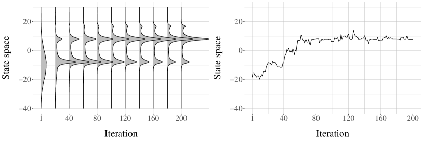
Figure 1: Convergence of the marginal distribution $\pi_{t}$ to $\pi$ (left) and a realized trajectory (right), here generated by a Metropolis–Rosenbluth–Teller–Hastings (MRTH) algorithm with Normal random walk proposals. The target distribution is described in Example 3.1 of Robert, (1995). This setting is used for all illustrations of this document.

Despite its asymptotic disappearance, the initialization bias poses practical issues. The bias is an obstacle to the parallelization of MCMC computation (Rosenthal,, 2000). Indeed, users can generate short MCMC runs independently in parallel, but the bias prevents the consistent estimation of $\pi(h)$ by averages over the independent runs. The bias can be reduced by discarding a larger initial portion of each parallel run, but the choice of the length to discard is both difficult and critical. This is in part because a sufficient length for the bias to be small is vastly different from one application to the next; numbers of iterations reported in the literature span many orders of magnitude, e.g. Metropolis et al., (1953) perform a few dozen sweeps whereas McCartan and Imai, (2023) mention a run of a trillion ($10^{12}$) MCMC iterations for the task of sampling redistricting plans.

1.2 The promise of unbiased MCMC

Unbiased MCMC removes the initialization bias. The key requirement of these methods is that the user can generate certain couplings of Markov chains (see Section 1.3). This requirement is weaker than that of Coupling From The Past (Propp and Wilson,, 1996), and thus unbiased MCMC is more widely applicable; but it does not provide perfect samples from $\pi$. Instead, these methods pioneered by Glynn and Rhee, (2014) generate unbiased approximations of $\pi$ in the form of signed empirical measures:

$$\hat{\pi}=\sum_{n=1}^{N}\omega_{n}\delta_{Z_{n}},$$ (1.3)

where $N$ is a random integer, $(Z_{n})_{n=1}^{N}$ are atoms on the state space $\mathbb{X}$, and $(\omega_{n})_{n=1}^{N}$ are real-valued weights (see Section 2.4 for the precise construction). The lack-of-bias property of $\hat{\pi}$ means that, for a class of functions $h$, $\hat{\pi}(h):=\sum_{n=1}^{N}\omega_{n}h(Z_{n})$ has expectation exactly equal to $\pi(h)$. The significance of the lack of bias is that users can generate independent copies of $\hat{\pi}(h)$ in parallel and average over the copies to obtain consistent estimators of $\pi(h)$, converging at the standard Monte Carlo rate if the estimators have a finite variance. Theorem 2.1 below provides conditions under which this holds. The lack of bias is thus clearly appealing as a means toward a parallel-friendly consistent Monte Carlo scheme; there are other appeals discussed in Section 5.

With unbiased signed measures, the question of initialization bias seems to be resolved. However, both the computing time and the variance can be prohibitively high. To quantify the price of removing the bias, for any function $h$, we can compute the inefficiency, a key descriptor of asymptotic performance for unbiased estimators (Glynn and Whitt,, 1992), defined as the expected computing cost multiplied by the variance of $\hat{\pi}(h)$. Both the expected cost and the variance can be estimated from independent runs. Meanwhile, the standard MCMC estimator has a cost proportional to the number of iterations $t$, and a variance of order $v(P,h)/t$ as $t\to\infty$, with $v(P,h)$ the asymptotic variance in the CLT (1.2). Thus, the asymptotic inefficiency of MCMC is measured by $v(P,h)$. The first unbiased estimators constructed from coupled chains in Glynn and Rhee, (2014), with MCMC applications presented in Agapiou et al., (2018), were not always competitive with MCMC in terms of asymptotic inefficiency. The simple enhancements proposed in Jacob et al., 2020a ; Jacob et al., 2020b ; Vanetti and Doucet, (2020) (see Section 2.3) led to unbiased MCMC estimators that are nearly as efficient as standard MCMC estimators in a wide range of settings.

1.3 Successful couplings of Markov chains

Unbiased MCMC belongs to a family of algorithms that require couplings of Markov chains, as in Coupling From The Past (CFTP, see Propp and Wilson, (1996)), circularly-coupled MCMC (Neal,, 1999), and Johnson’s convergence diagnostics (Johnson,, 1996, 1998). A coupling of two distributions $p$ and $q$ on $\mathbb{X}$ refers to a joint distribution on $\mathbb{X}\times\mathbb{X}$, with prescribed marginals $p$ and $q$. For Markov chains, a coupling refers to a joint process $(X_{t},Y_{t})$ such that $(X_{t})$ and $(Y_{t})$ are individually identical to prescribed Markov chains. For simplicity, we focus on Markovian couplings, where $(X_{t},Y_{t})$ itself forms a Markov chain, with initial distribution $\bar{\pi}_{0}$ on $\mathbb{X}\times\mathbb{X}$ and Markov transition $\bar{P}$.

1. Sample $(X_{0},Y_{0})$ from $\bar{\pi}_{0}$, .

2. If $L\geq 1$, for $t=1,\ldots,L$, sample $X_{t}$ from $P(X_{t-1},\cdot)$.

3. For $t\geq L$, sample $(X_{t+1},Y_{t-L+1})$ from $\bar{P}((X_{t},Y_{t-L}),\cdot)$ until $X_{t+1}=Y_{t-L+1}$ and $t+1\geq\ell$.

Algorithm 1 Successful coupling of chains with lag $L$ and length $\ell$. Coupled initial distribution: $\bar{\pi}_{0}$, transition: $P$, coupled transition: $\bar{P}$, meeting time: $\tau=\inf\{t\geq L:X_{t}=Y_{t-L}\}$.

Unbiased MCMC requires draws of $(X_{t},Y_{t})$ such that both chains $(X_{t})$ and $(Y_{t})$ are copies of the same Markov process that has initial distribution $\pi_{0}$, and transition $P$. Thus, $\bar{\pi}_{0}$ should be a coupling of $\pi_{0}$ with itself: $\bar{\pi}_{0}(A\times\mathbb{X})$ and $\bar{\pi}_{0}(\mathbb{X}\times A)$ should equal $\pi_{0}(A)$ for any measurable set $A$. The transition $\bar{P}$ should be a coupling of $P$ with itself: $\bar{P}((x,y),A\times\mathbb{X})$ and $\bar{P}((x,y),\mathbb{X}\times A)$ should equal $P(x,A)$ and $P(y,A)$ respectively for all $A$. Furthermore, for each trajectory of $(X_{t},Y_{t})$ we require the existence of a finite meeting time $\tau$ such that $X_{t}=Y_{t-L}$ for all $t\geq\tau$, where $L\geq 1$ is a user-chosen lag parameter. Coupling resulting in finite meeting times are called successful in this document, following Pitman, (1976). The construction is described in Algorithm 1. A realization of a successful coupling is shown in Figure 2, where $L=50$ and $\ell=500$.

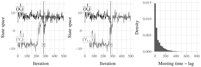
Figure 2: Successful coupling of Markov chains, meeting at time $\tau$ with a lag $L$: $X_{t}=Y_{t-L}$ for all $t\geq\tau$. Left: trajectory of $(X_{t},Y_{t})$. Middle: trajectory of $(X_{t},Y_{t-L})$. Right: histogram of $10^{4}$ independent copies of $\tau-L$.

The key assumption in this document is about the tails of the meeting times associated with coupled chains started from an independent coupling of $\pi$ and $\pi$, and propagated according to $\bar{P}$. Thus, the assumption does not involve $\pi_{0}$. The assumption is taken from Douc et al., (2023) and is equivalent to $\mathbb{P}(\tau>t)$ decaying at a polynomial rate as $t\to\infty$.

Assumption 1.

There exists $\kappa\geq 1$ such that, if two chains $(X_{t})$ and $(Y_{t})$ start from $\pi$ independently, and evolve according to $\bar{P}$, the meeting time $\tau=\inf\{t\geq 1:X_{t}=Y_{t}\}$ satisfies $\mathbb{E}[\tau^{\kappa}]<\infty$.

The assumption has implications on the marginal chain. For example, it implies that the CLT in (1.2) holds for any $h\in L^{p}(\pi)$ with $p>2\kappa/(\kappa-1)$ (Douc et al.,, 2023). The assumption is useful to study unbiased MCMC estimators as illustrated in Theorems 2.1 and 2.2 below.

Assumption 1 can be verified in different ways, on a case-by-case basis. If the transition $P$ satisfies a Lyapunov drift condition with function $V$, and if $\bar{P}$ results in a non-zero probability of meeting over one step when both chains are simultaneously in a level set of $V$, then Section 3.2 in Jacob et al., 2020b provides a result on the tails of $\tau$. That result applies in the numerous cases where explicit Lyapunov functions have already been elicited: random walk Metropolis–Rosenbluth–Teller–Hastings, abbreviated MRTH (see Roberts and Tweedie,, 1996), Langevin Monte Carlo (Durmus and Moulines,, 2022), Hamiltonian Monte Carlo (Durmus et al.,, 2017), and many examples of Gibbs samplers. A similar result applies under polynomial drift conditions (Section 1.4 in Middleton et al.,, 2020).

As a concrete example, a simple random walk MRTH algorithm is implemented in R in Figure 3, where the function U represents $x\mapsto-\log\pi(x)$ up to an additive constant. It employs a coupling of Normal proposal distributions presented in Section 2.3 of Bou-Rabee et al., (2020), and in Section 4.1 below. This coupling was employed to generate all figures in this document. Assumption 1 can then be verified for all $\kappa>1$ via Proposition 4 in Jacob et al., 2020b using the geometric drift function $V(x)=\pi(x)^{-1/2}$ under the conditions of Theorem 3.2 in Roberts and Tweedie, (1996). Section 4 provides more discussion on the design of successful couplings of MCMC algorithms.

⬇

1# Metropolis-Rosenbluth-Teller-Hastings transition with Normal proposals

2mrth = function(x, U, sigma)

3{

4 # proposal = current location + Normal(0,sigma^2)

5 xprop = x + sigma * rnorm(length(x))

6 # log Uniform to accept/reject proposals

7 logu = log(runif(1))

8 # return state according to decision to accept or not

9 return(if (logu < (U(x) - U(xprop))) xprop else x)

10}

11# coupling of MRTH transition with Normal proposals

12coupledmrth = function(x, y, U, sigma)

13{

14 # draw proposals using maximal coupling of Bou-Rabee, Eberle and Zimmer (AAP 2020)

15 xstd = rnorm(length(x)) # standard Normal variables

16 z = (x - y) / sigma # length(sigma) could be 1 or length(x)

17 e = z / sqrt(sum(z^2)) # normalise

18 logu = log(runif(1))

19 sameprop = (logu < sum(dnorm(xstd + z, log = TRUE) - dnorm(xstd, log = TRUE)))

20 ystd = if (sameprop) xstd + z else xstd - 2 * sum(e * xstd) * e

21 # xprop is marginally Normal(x,sigma^2)

22 xprop = x + sigma * xstd

23 # yprop is marginally Normal(y,sigma^2)

24 yprop = y + sigma * ystd

25 # log Uniform to accept/reject proposals

26 logu = log(runif(1))

27 # decision to accept or not

28 xaccept = (logu < (U(x) - U(xprop)))

29 yaccept = (logu < (U(y) - U(yprop)))

30 # return state according to decision

31 return(list(nextx = if (xaccept) xprop else x,

32 nexty = if (yaccept) yprop else y,

33 nextxequalsnexty = sameprop && xaccept && yaccept))

34}

Figure 3: R code for MRTH algorithm with Normal random walk proposals, and a coupling of it. This defines the transition $P$ and coupled transition $\bar{P}$ required by Algorithm 1. Inputs: current states x and y, a potential function U corresponding to $x\mapsto-\log\pi(x)$, proposal standard deviation sigma (a scalar or a vector of the same length as x and y).

2 Unbiased MCMC

This section presents unbiased MCMC estimators, assuming that successful couplings can be implemented and deferring to Section 4 for more on the design of such couplings. We start with bias removal techniques in Section 2.1, re-derive unbiased MCMC via the Poisson equation in Section 2.2, and present more efficient versions in Sections 2.3-2.4. In Section 2.5 we comment on performance, cost, parallel computing and tuning.

2.1 Bias removal with a telescope

Randomized telescoping sums. Consider a quantity of interest expressed as the limit $b_{\infty}$ of a deterministic sequence $(b_{k})_{k\geq 0}$ as $k\to\infty$. Defining $b_{-1}=0$ and $a_{k}=b_{k}-b_{k-1}$ for $k\geq 0$, we can write $b_{\infty}$ as the series $\sum_{k=0}^{\infty}a_{k}$. Assume that the time to compute the $k$-th term in the sequence $(b_{k})_{k\geq 0}$ is equal to $k$. Can we estimate a series $\sum_{k=0}^{\infty}a_{k}$ without bias in finite time? The following reasoning appears in Glynn, (1983); Rychlik, (1990). Let $\xi$ be a random variable on $\{0,1,2\ldots\}$ with $p_{k}:=\mathbb{P}(\xi=k)>0$ for all $k\geq 0$, called the truncation variable. Then sample $\xi$ and compute: $G={a_{\xi}}/{p_{\xi}}$. If the expectation of $|G|$ is finite then $\mathbb{E}[G]=b_{\infty}$, and its expected cost is $\mathbb{E}[\xi]=\sum_{k\geq 0}k\,p_{k}$. The cost is smaller if $(p_{k})$ decay faster. However, the variance of $G$ involves $\mathbb{E}[G^{2}]=\sum_{k\geq 0}a_{k}^{2}/p_{k}$ which is smaller if $(p_{k})$ decay slower. Thus, the estimator $G$ can only have finite expected cost and finite variance if $(b_{k})$ converges fast enough and if $(p_{k})$ is chosen adequately. An alternative is to sample $\xi$ and then compute $H=a_{0}+\sum_{k=1}^{\xi}a_{k}/\mathbb{P}(\xi\geq k)$. The estimator $H$ also has expectation $b_{\infty}$, its cost is similar to that of $G$, but its variance is finite under weaker conditions than that of $G$. The estimators $G$ and $H$ are termed single term and coupled sum, and are discussed in detail in Rhee and Glynn, (2015); Vihola, (2018).

Bias removal in MCMC. Direct use of the above strategy to remove the bias of MCMC averages, where $b_{k}=k^{-1}\sum_{s=0}^{k-1}h(X_{s})$, is considered in McLeish, (2011). An immediate difficulty is that ergodic averages converge at the (slow) Monte Carlo rate, resulting in unbiased estimators that tend to have either a large cost or a large variance. The convergence of marginal distributions $\pi_{t}\to\pi$ e.g. in total variation is comparably faster. Using contractive couplings of Markov chains and exploiting the (fast) convergence of marginal distributions, Glynn and Rhee, (2014) propose a debiasing strategy with a truncation variable that determines the length of the coupled chains. Glynn and Rhee, (2014) also consider the case where one could sample from a measure that minorizes the Markov transition. In that case their coupling results in pairs of chains that meet exactly, thus providing a natural stopping criterion for the coupled chains, and removing the need for truncation variables. Agapiou et al., (2018) employ contractive couplings of certain MCMC algorithms to obtain unbiased estimators and describe the practical choices associated with the specification of the truncation variable. Jacob et al., 2020a find that the conditional particle filter, which is an MCMC algorithm for continuous state space models (Andrieu et al.,, 2010), could be coupled such that a pair of chains would meet, often quickly, without the need for a truncation variable. Jacob et al., 2020b find that many MCMC algorithms can be coupled in that way, i.e. successfully, using maximal couplings as in Johnson, (1998). In this document we will focus on unbiased estimators obtained from successful couplings, where chains meet exactly, and truncation variables are not required.

First unbiased MCMC estimator. The idea of Glynn and Rhee, (2014) in the context of successful couplings introduced in Section 1.3 goes as follows. Write $\pi(h)$ as a telescopic sum, for all $k\geq 0$, for any choice of lag $L$,

$$\pi(h)=\lim_{t\to\infty}\pi_{t}(h)=\pi_{k}(h)+\sum_{j=1}^{\infty}\pi_{k+jL}(h)-\pi_{k+(j-1)L}(h).$$ (2.1)

For all $t\geq 0$, $X_{t}$ and $Y_{t}$ have the same distribution $\pi_{t}$, thus $\pi_{k+jL}(h)=\mathbb{E}[h(X_{k+jL})]$ and $\pi_{k+(j-1)L}(h)=\mathbb{E}[h(Y_{k+(j-1)L})]$. A swap of expectation and limit suggests that

$$H_{k}:=h(X_{k})+\sum_{j=1}^{\infty}(h(X_{k+jL})-h(Y_{k+(j-1)L})),$$ (2.2)

is an unbiased estimator of $\pi(h)$. For instance, if $|h|\leq 1$ then $\sum_{j=1}^{\infty}|h(X_{k+jL})-h(Y_{k+(j-1)L})|\leq 2\max(0,(\tau-k)/L)$. Therefore, if Assumption 1 holds with $\kappa=1$, then by Fubini’s theorem $H_{k}$ indeed satisfies $\mathbb{E}[H_{k}]=\pi(h)$. Higher moments of $H_{k}$ can be controlled as in Theorem 2.1 below. The infinite sum in (2.2) can be computed in finite time since the differences $h(X_{k+jL})-h(Y_{k+(j-1)L})$ are equal to zero for all $j$ such that $k+jL\geq\tau$.

2.2 Alternative construction via the Poisson equation

Poisson equation and bias. Douc et al., (2023) provide an alternative derivation of $H_{k}$ in (2.2) via the Poisson equation. Write $Pf(x)=\int P(x,dx^{\prime})f(x^{\prime})$ for a function $f:\mathbb{X}\to\mathbb{R}$. A function $g$ in $L^{1}(\pi)$ is a solution of the Poisson equation associated with $h$ and $P$ if

$$g(x)-Pg(x)=h(x)-\pi(h)\quad\forall x\in\mathbb{X}.$$ (2.3)

For example, the function

$$g_{\star}:x\mapsto\sum_{t=0}^{\infty}P^{t}\left\{h-\pi(h)\right\}(x),$$ (2.4)

may be a solution to (2.3) if it is well-defined; see Chapter 21 of Douc et al., (2018). As noted in Douc et al., (2023), if $h\in L^{p}(\pi)$ and if $\kappa$ in Assumption 1 is such that $p>2\kappa/(\kappa-1)$, then $g_{\star}$ is indeed in $L^{1}(\pi)$. In that case, all solutions to (2.3) are equal to $g_{\star}$ up to an additive constant. It is known that (2.4) is related to MCMC bias. Indeed, consider the ergodic average $t^{-1}\sum_{s=0}^{t-1}h(X_{s})$ when the chain starts from a fixed $x_{0}\in\mathbb{X}$. The bias is $\mathbb{E}_{x_{0}}[t^{-1}\sum_{s=0}^{t-1}h(X_{s})]-\pi(h)$, and if we multiply by $t$ and consider the limit $t\to\infty$,

$$\lim_{t\to\infty}t\times\{\mathbb{E}_{x_{0}}[t^{-1}\sum_{s=0}^{t-1}h(X_{s})]-\pi(h)\}=\lim_{t\to\infty}\sum_{s=0}^{t-1}\mathbb{E}_{x_{0}}[h(X_{s})-\pi(h)]=g_{\star}(x_{0}),$$ (2.5)

with $g_{\star}$ as in (2.4), and $\mathbb{E}_{x_{0}}$ referring to expectations with respect to the chain started from $X_{0}=x_{0}$ (Kontoyiannis and Dellaportas,, 2009).

Estimation of $g$ and unbiased MCMC. Consider the function $x\mapsto g(x,y):=g_{\star}(x)-g_{\star}(y)$, equal to $g_{\star}$ up to the constant $g_{\star}(y)$, for any fixed $y\in\mathbb{X}$, and thus solution of the Poisson equation under the aforementioned conditions. This solution can be written

$$g(x,y)=\sum_{t\geq 0}\{P^{t}h(x)-P^{t}h(y)\}.$$ (2.6)

Consider chains coupled successfully with no lag ($L=0$), started from $X_{0}=x$ and $Y_{0}=y$. Then $h(X_{t})$ and $h(Y_{t})$ have expectation equal to $P^{t}h(x)$ and $P^{t}h(y)$ for all $t\geq 0$, but for $t$ larger than $\inf\{t\geq 1:X_{t}=Y_{t}\}$ we have $h(X_{t})-h(Y_{t})=0$. This suggests the following unbiased estimator of $g(x,y)$:

$$G(x,y):=\sum_{t=0}^{\tau-1}\{h(X_{t})-h(Y_{t})\},$$ (2.7)

where here $\tau=\inf\{t\geq 1:X_{t}=Y_{t}\}$. With the ability to estimate solutions of the Poisson equation we might envision the estimation of $\pi(h)$ via the re-arranged equation: $\pi(h)=h(x)+Pg(x)-g(x)$. Setting $x\in\mathbb{X}$ arbitrarily, sample $X_{1}\sim P(x,\cdot)$ (performing one step of MCMC), and sample $G(X_{1},x)$ (running two chains, initialized at $X_{1}$ and $x$, until they meet). Then $\mathbb{E}_{x}[G(X_{1},x)]=Pg_{\star}(x)-g_{\star}(x)$, therefore $h(x)+G(X_{1},x)$ is an unbiased estimator of $\pi(h)$. It is in fact exactly $H_{k}$ in (2.2) with $k=0$, $L=1$ and $\pi_{0}=\delta_{x}$.

2.3 Unbiased MCMC estimators

Improved efficiency by averaging. Simple modifications of (2.2) can go a long way to improve its efficiency, as noted in Jacob et al., 2020a ; Jacob et al., 2020b . Consider a run of Algorithm 1 with lag $L\geq 1$ (Vanetti and Doucet,, 2020) and length $\ell\geq 0$, from which we can construct unbiased estimators $H_{k},\ldots,H_{\ell}$ as in (2.2) for a range of integers $k,\ldots,\ell$ where $0\leq k\leq\ell$. Since these estimators $(H_{t})_{t=k}^{\ell}$ are unbiased, their average is unbiased as well. We define

$$H_{k:\ell}=\frac{1}{\ell-k+1}\sum_{t=k}^{\ell}H_{t}.$$ (2.8)

After some algebraic manipulations, that estimator reads

$$H_{k:\ell}=\underbrace{\frac{1}{\ell-k+1}\sum_{t=k}^{\ell}h(X_{t})}_{\text{MCMC}}+\underbrace{\sum_{t=k+L}^{\tau-1}v_{t}(k,\ell,L)\left\{h(X_{t})-h(Y_{t-L})\right\}}_{\text{bias cancellation}},$$ (2.9)

with weights $v_{t}(k,\ell,L)$ defined precisely below. In (2.9) the sum $\sum_{t=k+L}^{\tau-1}$ is zero if $k+L\geq\tau$. The first term on the right-hand side is the regular MCMC ergodic average, computed from the trajectory $(X_{k},\ldots,X_{\ell})$. The second term performs bias cancellation from weighted differences between the chains. The weight $v_{t}(k,\ell,L)$ is defined as the number of appearances of the difference $h(X_{t})-h(Y_{t-L})$ in the bias cancellation terms of $H_{k},\ldots,H_{\ell}$, divided by $\ell-k+1$. Note that, for two positive integers $a\leq b$, the number of multiples of $L$ within $\{a,\ldots,b\}$ equals $\lfloor b/L\rfloor-\lceil a/L\rceil+1$. Using this and routine calculations, the weight can be written as

$$v_{t}(k,\ell,L)=\frac{\lfloor(t-k)/L\rfloor-\lceil\max(L,t-\ell)/L\rceil+1}{\ell-k+1}.$$ (2.10)

Both the number of terms in the bias cancellation and their weights can be reduced by increasing the tuning parameters $k,\ell,L$. This impacts the cost of obtaining $H_{k:\ell}$: indeed, if we count the cost of sampling from the MCMC transition $P$ as one unit, and the cost of sampling from the coupled transition $\bar{P}$ as one unit if the chains have already met and two units if they have not, then

$$\text{cost}(H_{k:\ell})=L+2(\tau-L)+\max(0,\ell-\tau).$$ (2.11)

Section 2.5 proposes guidance on tuning unbiased MCMC, and Figure 5 provides an illustration of the effect of tuning.

Variance reduction. The estimator in (2.9) is presented with a generic lag $L$ following the observation of Vanetti and Doucet, (2020) that increasing $L$ can lead to significant variance reduction. Control variates for $H_{k:\ell}$ are proposed in Craiu and Meng, (2022). They observe that $\mathbb{E}[h(X_{t})-h(Y_{t})]=0$ for all $t\geq 0$, thus $\sum_{t\geq 0}\eta_{t}\{h(X_{t})-h(Y_{t})\}$ can be added to $H_{k:\ell}$, for any real sequence $(\eta_{t})$, without modifying its expectation. Optimization over the sequence $(\eta_{t})$ can lead to a reduction in variance. Other coupling-based variance reduction strategies have been proposed for MCMC (Neal and Pinto,, 2001), as well as techniques related to the Poisson equation (Andradóttir et al.,, 1993; Alexopoulos et al.,, 2023).

Finite moments. The following result is taken from Douc et al., (2023). It assumes that $\pi_{0}$ has bounded Radon–Nikodym derivative with respect to $\pi$. For example, if $\pi$ is continuous and strictly positive on $\mathbb{R}^{d}$, then the assumption rules out the choice of $\pi_{0}$ as a Dirac mass, but it allows $\pi_{0}$ to be the Uniform distribution on any ball with positive radius.

Theorem 2.1.

Under Assumption 1 with $\kappa>1$, i.e. $\mathbb{E}[\tau^{\kappa}]<\infty$, let $h\in L^{m}(\pi)$ for some $m>\kappa/(\kappa-1)$. Assume that $\pi_{0}$ is such that $d\pi_{0}/d\pi\leq M$ with $M<\infty$. Then for any $k,\ell,L$, the estimator $H_{k:\ell}$ in (2.9) is unbiased: $\mathbb{E}[H_{k:\ell}]=\pi(h)$, and satisfies $\mathbb{E}[|H_{k:\ell}|^{p}]<\infty$ for $p\geq 1$ such that $\frac{1}{p}>\frac{1}{m}+\frac{1}{\kappa}$.

Finiteness of the first two moments is particularly useful. Finiteness of the variance of $H_{k:\ell}$ is sufficient to validate the following classical construction of confidence intervals: generate $C$ independent copies of $H_{k:\ell}$, compute their average $\hat{\mu}$ and their standard deviation $\hat{\sigma}$, and an asymptotically (as $C\to\infty$) valid confidence interval for $\pi(h)$ is given by $[\hat{\mu}+q_{\alpha/2}\hat{\sigma}/\sqrt{C},\hat{\mu}+q_{1-\alpha/2}\hat{\sigma}/\sqrt{C}]$, where $q_{s}$ is the $s$-th quantile of the standard Normal distribution. According to Theorem 2.1, finiteness of second moments ($p=2$) holds under a mild condition on $\pi_{0}$, the assumption that $\kappa>2$ and for all $h\in L^{m}(\pi)$ such that $m>2\kappa/(\kappa-2)$. If $\tau$ has Geometric tails, then $\kappa$ can be taken arbitrary large, and the result holds for all $h\in L^{2+\eta}(\pi)$ for any $\eta>0$.

2.4 Unbiased signed measure

Replacing function evaluations by Dirac masses. The empirical measure

$$\hat{\pi}({\rm d}x)=\underbrace{\frac{1}{\ell-k+1}\sum_{t=k}^{\ell}\delta_{X_{t}}({\rm d}x)}_{\text{MCMC}}+\underbrace{\sum_{t=k+L}^{\tau-1}v_{t}(k,\ell,L)\left\{\delta_{X_{t}}-\delta_{Y_{t-L}}\right\}({\rm d}x)}_{\text{bias cancellation}},$$ (2.12)

is an unbiased approximation of $\pi$, where $v_{t}$ is defined in (2.10). This is of the form $\sum_{n=1}^{N}\omega_{n}\delta_{Z_{n}}$ as in (1.3), with $N=\max(0,\tau-(k+L))+(\ell-k+1)$, $Z_{n}$ are states from either $(X_{t})$ or $(Y_{t})$ and $\omega_{n}$ are either $(\ell-k+1)^{-1}$, or of the form $\pm v_{n}(k,\ell,L)$; in particular the weights can be negative. Figure 4 represents the unbiased MCMC approximation, made of MCMC and bias cancellation components. This figure was created using kernel density estimation from the weighted samples constituting the different elements in (2.12).

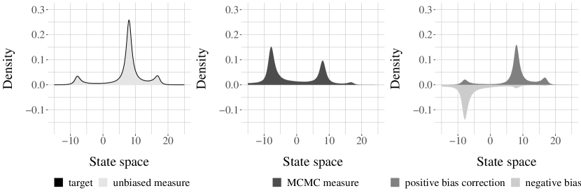
Figure 4: Unbiased MCMC (left) = MCMC (middle) + bias cancellation (right). The target density is the black curve on the left-most plot. On the right, the bias cancellation is made of a positive measure (darker grey) added to a negative measure (lighter grey).

Sub-sampling and negative weights. We can sub-sample from the empirical measure in (1.3). For example, we can draw an index $I$ uniformly in $\{1,\ldots,N\}$ and return the sample $Z_{I}$ with weight $N\omega_{I}$. Then for a class of functions $h$, $N\omega_{I}h(Z_{I})$ will have expectation equal to $\pi(h)$ (Douc et al.,, 2023). We can also sample the index $I$ non-uniformly, with probabilities $\xi_{1},\ldots,\xi_{N}$ that depend on the atoms in (1.3), and the selected atom $Z_{I}$ is then weighted by $\xi_{I}^{-1}\omega_{I}$, and we may repeat this selection multiple times to obtain a weighted sub-sample from (1.3) with a desired size. Yet this does not produce a perfect sample due to the weights being possibly negative. We can arbitrarily decrease the proportion of negative weights in (1.3) by increasing the value of $k$, but we cannot make it zero. As a result, unbiased MCMC estimators $H_{k:\ell}$ can take values outside the range of the function $h$, e.g. we may obtain negative estimates of positive quantities. There may not be any general solution to this problem: according to Lemma 2.1 in Jacob and Thiery, (2015) there is no algorithm that takes unbiased estimators of a nonnegative quantity as input (and nothing else), and returns nonnegative unbiased estimators of that same quantity.

2.5 Efficiency, cost and tuning

Asymptotic equivalence with MCMC. Theorem 2.1 validates unbiased MCMC for the estimation of $\pi(h)$ but does not help for the comparison of its performance with standard MCMC, or the choice of the tuning parameters $k,\ell,L$. The guiding principle in the tuning of $k,\ell,L$ is that a judicious choice will make unbiased MCMC competitive with standard MCMC in terms of cost and variance. Proposition 3 in Jacob et al., 2020b provides conditions under which the increase of either $k$ or $\ell-k$ results in variance reduction, and in particular the variance of $H_{k:\ell}$ is shown to be asymptotically equivalent to the variance of standard MCMC estimators as $\ell\to\infty$. The result is shown under weaker conditions in Middleton et al., (2020). In the same spirit Douc et al., (2023) provide the following CLT for $H_{k:\ell}$ as $\ell\to\infty$, where the asymptotic variance is the same as for standard MCMC.

Theorem 2.2.

Under Assumption 1 with $\kappa>1$, let $h\in L^{m}(\pi)$ for some $m>2\kappa/(\kappa-1)$. Then for any $k\in\mathbb{N}$,

$$\sqrt{\ell-k+1}\left(H_{k:\ell}-\pi(h)\right)\overset{d}{\to}\text{Normal}(0,v(P,h)),$$ (2.13)

as $\ell\to\infty$, where $v(P,h)$ is the asymptotic variance in the CLT for MCMC averages (1.2).

The asymptotic equivalence with regular MCMC as $\ell\to\infty$ should be expected since the initialization bias vanishes as $\ell\to\infty$. It can be seen in the form of the bias cancellation term in (2.9): the sum is over $\max(0,\tau-L-k)$ terms (irrespective of $\ell$) and the weights in (2.10) decrease as $(\ell-k)^{-1}$. Thus, the bias cancellation term disappears when $\ell-k$ increases. The cost of $H_{k:\ell}$ in (2.11) behaves as $\ell$ when $\ell\to\infty$. Hence, both cost and variance of $H_{k:\ell}$ are equivalent to those of MCMC as $\ell\to\infty$. By carefully choosing $k,\ell,L$ we can obtain unbiased MCMC estimators with an efficiency close to that of MCMC.

Cost and parallel computing. Efficiency is not the only criterion when tuning unbiased MCMC. Some users might prefer less efficient but cheaper estimators when enough parallel machines are available to produce them. Consider generating $C$ estimates on $M$ parallel machines. When $M\ll C$, each machine produces many of the $C$ estimates. The speed-up of using $M$ parallel machines is then close to linear in $M$. On the other hand, if $M\geq C$, each machine produces one estimate, and the user must wait for the longest run to complete. Careful: running unbiased MCMC on $M\gg C$ machines and retaining the $C$ estimators that are first completed would introduce a bias, since the estimator is not independent of its cost. Figure 5 (left) illustrates the chronology of the generation of independent estimators on parallel machines, with each machine producing a random number of estimators within a given time period. If each machine is tasked to produce a single estimator, the total time is exactly the (random) cost of the longest run, which behaves in average as an increasing function of the number of machines (see relevant discussions in Wang et al., (2024)). For example if $\tau$ has Geometric tails, the average maximum cost of unbiased MCMC behaves as $\log(C)$. Handling of budget constraints, such as hard or soft deadlines, on parallel machines is discussed in Glynn and Heidelberger, (1990, 1991); Jacob et al., 2020b .

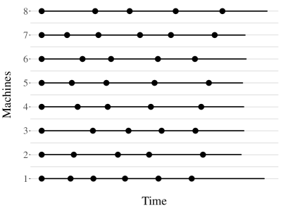
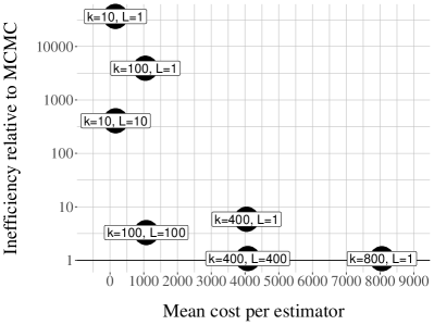
Figure 5: Left: chronology of the generation of estimators on parallel machines, with each dot representing the start of a run. Right: inefficiency of unbiased MCMC divided to the inefficiency of MCMC, versus mean cost of $H_{k:\ell}$, for different choices of $k$, and $L$ set to either $1$ or $k$, always with $\ell=10k$. The configuration $k=800,L=800$ is not shown as it would be overlaid with $k=800,L=1$.

Choice of length $\ell$. We proceed to proposing guidance for the tuning parameters. First we simplify the choice by recommending that $\ell$ is set as a large multiple of $k$, for example $\ell=10k$. This is because a portion $k/\ell$ of iterations is simply discarded in the construction of (2.9), and we would like to limit this apparent waste. Thus, we are left with the choice of $k$ and $L$; increasing $k$ will automatically increase $\ell$ and $\ell-k$, thus decreasing the magnitude of the weights $v_{t}$ in the bias cancellation term.

Choice of burn-in $k$ and lag $L$. The bias cancellation is exactly zero in the event $\{\tau-L<k\}$. By setting $k$ as a large quantile of $\tau-L$, we ensure that the event occurs with high probability. The increase of the lag $L$, compared to the choice $L=1$ in Glynn and Rhee, (2014); Jacob et al., 2020b , is advocated in Vanetti and Doucet, (2020). From the expression of the weights in (2.10), increasing $L$ decreases the weights in the bias cancellation term, and thus brings $H_{k:\ell}$ closer to regular MCMC. Furthermore, setting $L=k$ leads to a minor increase of cost per estimator compared to $L=1$, and thus the efficiency is typically improved, sometimes drastically.

Concrete guideline. In our experience, satisfactory tuning can be done as follows. First generate independent meeting times with lag $L=1$ (by lack of a better guess). Then set $k$ as a large (e.g. $99\%$) quantile of $\tau-L$, which is the number of coupled transitions up to the meeting time. Finally, redefine $L=k$, and set $\ell=10k$. Figure 5 (right) shows how different choices of $k,L$ (always with $\ell=10k$) lead to vastly different costs and inefficiencies, for the estimation of $\pi(h)$ with $h:x\mapsto x$. In the figure, the inefficiency of unbiased MCMC is divided by the asymptotic variance $v(P,h)$ of MCMC, estimated using the method of Section 3.2. The relative inefficiency becomes close to one when $\ell=10k$ increases, and setting $L=k$ instead of $L=1$ is often worthwhile.

3 Beyond the estimation of stationary expectations

Unbiased MCMC provides estimators of stationary expectations $\pi(h)$, and also helps in addressing questions of interest to MCMC users, including non-asymptotic convergence diagnostics (Section 3.1), and efficiency comparisons (Section 3.2).

3.1 Convergence diagnostics

Total variation distance to stationarity. As a by-product of the unbiased estimator in (2.2) we can construct upper bounds on the total variation distance $|\pi_{k}-\pi|_{\text{TV}}$, for any finite $k$, that can be estimated from samples of meeting times, as first proposed in Section 6 of Jacob et al., 2020b , and improved with the use of $L>1$ in Biswas et al., (2019), and with control variates in Craiu and Meng, (2022). A simple way of deriving such bounds is to write, for any $k\geq 0$,

$$|\pi_{k}-\pi|_{\text{TV}}=\inf_{(X_{k},X)\in\Gamma(\pi_{k},\pi)}\mathbb{E}[\mathds{1}(X_{k}\neq X)],$$ (3.1)

where the infimum is over the set $\Gamma(\pi_{k},\pi)$ of all pairs of variables $(X_{k},X)$ where $X_{k}\sim\pi_{k}$ and $X\sim\pi$. First use the triangle inequality to obtain an upper bound of the form $\sum_{j=1}^{\infty}|\pi_{k+jL}-\pi_{k+(j-1)L}|_{\text{TV}}$, and then use the pair $(X_{k+jL},Y_{k+(j-1)L})$ generated by Algorithm 1 to obtain an upper bound $\mathbb{E}[\mathds{1}(X_{k+jL}\neq Y_{k+(j-1)L})]$ on each term in the sum. Thus, a swap of expectation and limit yields

$$|\pi_{k}-\pi|_{\text{TV}}\leq\mathbb{E}[\sum_{j=1}^{\infty}\mathds{1}(X_{k+jL}\neq Y_{k+(j-1)L})]=\mathbb{E}[\max(0,\lceil(\tau-L-k)/L\rceil)].$$ (3.2)

The right-hand side is obtained by counting the indices $j\geq 1$ such that $k+jL$ is within $\{L,\ldots,\tau-1\}$. The bounds can be estimated by replacing the expectation by an empirical average over $C$ independent meeting times $\tau_{1},\ldots,\tau_{C}$, for any value of $k$. Thus one can run Algorithm 1 with lag $L$ and $\ell=0$, $C$ times independently. The empirical upper bound $C^{-1}\sum_{c=1}^{C}\max(0,\lceil(\tau_{c}-L-k)/L\rceil)$ is exactly zero for all $k\geq\max_{c}\tau_{c}-L$, so it is enough to evaluate it at integers $k$ less than $\max_{c}\tau_{c}-L$. Figure 6 (left) shows these bounds obtained for three different lags. Increasing the lag tends to decrease the bounds, but the sharpness of the bounds also depends on the choice of coupling. To choose $L$, as before, we can first generate meeting times with $L=1$, and then redefine $L$ as a large (e.g. $99\%$) empirical quantile of $\tau-L$, the number of coupled transitions leading to the meeting time.

1-Wasserstein distance to stationarity. A similar reasoning leads to upper bounds on other distances that have a coupling representation. Biswas et al., (2019) consider the 1-Wasserstein distance, defined as

$$|\pi_{k}-\pi|_{W_{1}}=\inf_{(X_{k},X)\in\Gamma(\pi_{k},\pi)}\mathbb{E}[|X_{k}-X|],$$ (3.3)

where $|x-y|$ represents a distance between $x$ and $y$ such as the Euclidean distance on $\mathbb{R}^{d}$. With the same reasoning, first use the triangle inequality, and then employ any coupling of $\pi_{k+jL}$ and $\pi_{k+(j-1)L}$ for $j\geq 1$. Thus, by running Algorithm 1 with lag $L$ and $\ell=0$, assuming the validity of an exchange of expectation and limit, we obtain the upper bounds:

$$\forall k\geq 0\quad|\pi_{k}-\pi|_{W_{1}}\leq\mathbb{E}[\sum_{j=1}^{\lfloor(\tau-k-1)/L\rfloor}|X_{k+jL}-Y_{k+(j-1)L}|].$$ (3.4)

The sum on the right-hand side runs until $j$ such that $k+jL<\tau$, after which each term is zero. Figure 6 (right) represents these bounds for three different lags. As noted in Papp and Sherlock, 2022a , the $p$-th power of the $p$-Wasserstein distance between $\pi_{k}$ and $\pi$ can be upper bounded in the same way.

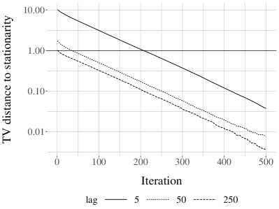
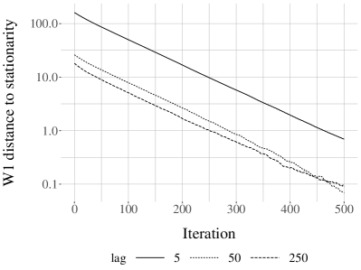
Figure 6: Left: upper bounds on $|\pi_{k}-\pi|_{\text{TV}}$ for different times $k$ on the x-axis, obtained using (3.2) and $10^{4}$ independent copies of meeting times associated with lags $5$, $50$ and 250. The total variation distance is always less than one. Right: similar plot but for the 1-Wasserstein distance, obtained using (3.4). The y-axes are on logarithmic scale.

Practical significance. We stress the usefulness of (3.2) or (3.4) compared to the usual bounds encountered in the literature on Markov chains. In continuous state spaces, the coupling inequality due to Wolfgang Doeblin (Lindvall,, 2002) reads: $|\pi_{k}-\pi|_{\text{TV}}\leq\mathbb{P}(\tau>k)$ for all $k\geq 0$, where the meeting time is that of a pair of chains (without any lag), started from $\pi_{0}$ and $\pi$, but MCMC users can rarely sample from $\pi$. In discrete state spaces, one can also write $\max_{x}|P^{k}(x,\cdot)-\pi|_{\text{TV}}\leq\max_{x,y}\mathbb{P}_{x,y}(\tau>k)$ where the meeting time corresponds to chains started from states $x,y$ (Corollary 5.3 in Levin and Peres,, 2017). Optimizing over the states $x,y$ could be computationally difficult. In contrast, the upper bounds described above involve pairs of chains started from an arbitrary $\pi_{0}$.

Limitation. As a warning, the following describes a situation where the use of (3.2) would fail to provide reliable bounds on $|\pi_{k}-\pi|_{\text{TV}}$. Suppose that the target $\pi$ is multimodal, and that chains tend to get stuck in local modes. Assume further that the initial distribution $\pi_{0}$ puts its mass entirely in a local mode of $\pi$. The user might then observe a small empirical average of the meeting time, even after many independent runs. Yet the expectation of the meeting time could be much larger. Indeed, there could be a small probability that one chain moves to a different mode before meeting the second chain, and in that event, the meeting time could take large values, driving the expectation upward. This is illustrated in Section 5.1 of Jacob et al., 2020b . The risk is mitigated by specifying an initial distribution $\pi_{0}$ that is spread out relative to the modes of $\pi$, or by increasing the lag $L$ (Biswas et al.,, 2019).

3.2 Efficiency comparison

Unbiased MCMC and its connection to the Poisson equation (Douc et al.,, 2023), see Section 2.2, lead to unbiased estimators of the asymptotic variance $v(P,h)$ in the CLT (1.2).

Asymptotic variance through the Poisson equation. A standard way of establishing the CLT for Markov chain averages (Douc et al.,, 2018, Chapter 21) is to write $\sum_{s=0}^{t-1}\{h(X_{s})-\pi(h)\}=\sum_{s=1}^{t}\left\{g(X_{s})-Pg(X_{s-1})\right\}+g(X_{0})-g(X_{t})$, where $g$ is a solution of the Poisson equation (2.3), and then to observe that $\left\{g(X_{s})-Pg(X_{s-1})\right\}_{s\geq 1}$ forms a martingale difference sequence. The CLT for martingale difference sequences and some routine calculations yield

$$v(P,h)=\mathbb{E}_{\pi}[\{g(X_{1})-Pg(X_{0})\}^{2}]=2\underbrace{\pi(\{h-\pi(h)\}g)}_{\text{(a)}}-\underbrace{(\pi(h^{2})-\pi(h)^{2})}_{\text{(b)}}.$$ (3.5)

From the above representation of $v(P,h)$, Douc et al., (2023) combine unbiased estimators $G$ of evaluations of $g$, from (2.7) in Section 2.2, with unbiased MCMC approximations $\hat{\pi}$ of $\pi$ as in (2.12), to deliver estimators $\hat{v}(P,h)$ with $\mathbb{E}[\hat{v}(P,h)]=v(P,h)$. The estimator in its simplest form goes as follows. First, run two independent unbiased MCMC estimators $\hat{\pi}^{(j)}$, for $j=1,2$, as in (2.12). Using $\hat{\pi}^{(1)},\hat{\pi}^{(2)}$ we can estimate without bias the term $(b)$ in (3.5) by

$$(B)=(\hat{\pi}^{(1)}(h^{2})+\hat{\pi}^{(2)}(h^{2}))/2-\hat{\pi}^{(1)}(h)\hat{\pi}^{(2)}(h).$$ (3.6)

To estimate $(a)$ in (3.5), recall from Section 2.2 that, for any $x$, we can run coupled chains to obtain an unbiased estimator $G(x,y)$ in (2.7) of $g(x,y)$ in (2.6), for any fixed choice of $y\in\mathbb{X}$. Then, write $\hat{\pi}^{(1)}$ in the form $\sum_{n=1}^{N}\omega_{n}\delta_{Z_{n}}$. Draw $I$ uniformly in $\{1,\ldots,N\}$, and run coupled chains started from $Z_{I}$ and $y$ to obtain $G(Z_{I},y)$. Conditioning on $\hat{\pi}^{(1)},\hat{\pi}^{(2)}$ and $I$, we have

$$\mathbb{E}\left[N\omega_{I}G(Z_{I},y)\left(h(Z_{I})-\hat{\pi}^{(2)}(h)\right)|\;\hat{\pi}^{(1)},\hat{\pi}^{(2)},I\right]=N\omega_{I}g(Z_{I},y)\left(h(Z_{I})-\hat{\pi}^{(2)}(h)\right).$$ (3.7)

By further averaging out $I$ we obtain $\hat{\pi}^{(1)}(g(\cdot,y)h)-\hat{\pi}^{(2)}(h)\hat{\pi}^{(1)}(g(\cdot,y))$, and since $\hat{\pi}^{(j)}$ for $j=1,2$ are unbiased, we see that

$$(A)=N\omega_{I}G(Z_{I},y)\left(h(Z_{I})-\hat{\pi}^{(2)}(h)\right),$$ (3.8)

is an unbiased estimator of $(a)$ in (3.5). Thus, $\hat{v}(P,h)=2(A)-(B)$ is an unbiased estimator of $v(P,h)$. This estimator can be improved in various ways, for instance by drawing multiple copies of $I$ and estimating the solution of the Poisson equation at the corresponding states $Z_{I}$. We refer the reader to Douc et al., (2023) for more details on such estimators.

Practical significance. The quantity $v(P,h)$ measures the efficiency of the underlying MCMC algorithm, and thus constitutes a reference value for the efficiency of unbiased MCMC, as seen in Section 2.5. Access to the unbiased estimators of $v(P,h)$ enables efficiency comparisons between standard and unbiased MCMC, such as that represented in Figure 5 (right), without ever performing long MCMC runs. Comparisons can also be done between MCMC algorithms, since the estimators are unbiased for the asymptotic variance, and are not upper bounds as in Section 3.1.

Under assumptions guaranteeing the existence of a finite variance for the unbiased estimator $\hat{v}(P,h)$ of $v(P,h)$, averages of $C$ independent copies would converge at the Monte Carlo rate. This compares favorably to classical estimators of $v(P,h)$ based on long runs. Indeed, commonly-used estimators of $v(P,h)$, such as batch means and spectral variance estimators, converge at a sub-Monte Carlo rate, e.g. $T^{-2/3}$ for batch means (Flegal and Jones,, 2010). A limitation of the unbiased estimation strategy is that it requires a successful coupling of the algorithm under consideration, whereas classical estimators only require trajectories of the chain.

4 Design of successful coupling of MCMC algorithms

To implement unbiased MCMC, users need to design a successful coupling of their MCMC algorithm. Focusing on Markovian couplings, this amounts to constructing a coupled transition $\bar{P}$ to plug in Algorithm 1 and for which Assumption 1 is satisfied. Concretely, we need to be able to sample $(X,Y)\sim\bar{P}((x,y),\cdot)$, where $(x,y)$ represent the current positions of the chains, such that 1) $X\sim P(x,\cdot)$ and $Y\sim P(y,\cdot)$, and 2) the resulting chains meet as quickly as possible. In Section 4.1 we review the more basic task of coupling random variables, before dealing with MCMC transitions in Section 4.2. References to realistic examples are provided in Section 4.3.

4.1 Couplings of random variables

Maximal couplings. A coupling of $(X,Y)$ with $X\sim p$ and $Y\sim q$ is maximal if $\mathbb{P}(X=Y)$ is maximal and thus equal to $1-|p-q|_{\text{TV}}$. There may be more than one maximal coupling. Algorithm 2 is a modification by Gerber and Lee, (2020) of the $\gamma$-coupling of Johnson, (1998) with an extra parameter $\eta\in(0,1]$. The scheme requires samples from $p$ and $q$, and evaluations of the ratio of their densities. The probability of $\{X=Y\}$ is maximal only when $\eta=1$. However, the cost of running Algorithm 2, which contains a while loop, has a variance that goes to infinity when $\eta=1$ and when $|p-q|_{\text{TV}}$ goes to zero. With $\eta<1$, the coupling is sub-maximal, but the variance of the cost is upper bounded uniformly over $p$ and $q$. Under Algorithm 2, conditionally on $Y$ being generated in step 2.(b), $X$ is independent of $Y$.

1. Sample $X\sim p$.

2. Sample $W\sim\text{Uniform}(0,1)$.

   1. If $W\leq\min(\eta,q(X)/p(X))$, set $Y=X$.

   2. Otherwise sample $Y^{\star}\sim q$ and $W^{\star}\sim\text{Uniform}(0,1)$ until $W^{\star}>\eta p(Y^{\star})/q(Y^{\star})$,

   3. and set $Y=Y^{\star}$.

3. Return $(X,Y)$.

Algorithm 2 Sampling a coupling of $p$ and $q$, with parameter $\eta\in(0,1]$. The coupling maximizes $\mathbb{P}(X=Y)$ when $\eta=1$, but the variance of the cost is bounded when $\eta<1$.

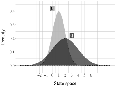
Figure 7: Left: distributions $p$ and $q$ defined as $\text{Normal}(\mu_{1},\sigma_{1}^{2})$, with $\mu_{1}=1,\sigma_{1}=1$, and $\text{Normal}(\mu_{2},\sigma_{2}^{2})$, with $\mu_{2}=2,\sigma_{2}=2$. Right: samples $(x_{i},y_{i})$ following a maximal coupling of $p$ and $q$ using Algorithm 2, shown as a scatter plot with marginal histograms.

Algorithm 3 samples the same pairs $(X,Y)$ as Algorithm 2 with $\eta=1$, but via a mixture representation; see e.g. Devroye, (1990); Brémaud, (1992), and Chapter 1 in Thorisson, (2000). Algorithm 3 is applicable when $\int\min(p(x),q(x))dx$ can be computed, and when $\tilde{p}$ and $\tilde{q}$ defined on line 3 can be sampled from. Note that $|p-q|_{\text{TV}}=1-\int\min(p(x),q(x))dx$. Its appeal is that its cost is deterministic. Maximal couplings are illustrated in Figure 7 in the case of two univariate Normal distributions. The figure shows the two probability density functions (left), and a sample of pairs $(x_{i},y_{i})$ generated using Algorithm 2 with $\eta=1$. Notably, some pairs $(x_{i},y_{i})$ are such that $x_{i}=y_{i}$.

1. Draw $U\sim\text{Uniform}(0,1)$ and compute $c=\int\min(p(x),q(x))dx$.

2. If $U\leq c$, draw $X\sim\nu$ with $\nu:x\mapsto\min(p(x),q(x))/c$, and set $Y=X$.

3. Otherwise, draw $X$ from $\tilde{p}:x\mapsto(p(x)-\min(p(x),q(x)))/(1-c)$,

4. and independently draw $Y$ from $\tilde{q}:x\mapsto(q(x)-\min(p(x),q(x)))/(1-c)$.

5. Return $(X,Y)$.

Algorithm 3 Sampling a maximal coupling of $p$ and $q$ via a mixture.

Synchronous couplings. The above algorithms generate $X$ and $Y$ independently, conditionally on the event that the draw of $X$ is not accepted for $Y$. Thus they revert to the independent coupling when $|p-q|_{\text{TV}}$ is close to one. A natural way of introducing dependencies among random variables is to use common random numbers to generate them. In one dimension, if $X$ has quantile function $F_{p}^{-}$ and $Y$ has quantile function $F_{q}^{-}$, then one can sample $U\sim\text{Uniform}(0,1)$ and set $X=F_{p}^{-}(U)$ and $Y=F_{q}^{-}(U)$. The resulting joint distribution minimizes $\mathbb{E}[(X-Y)^{2}]$, or equivalently, maximizes $\mathbb{C}\text{ov}(X,Y)$ (Glasserman and Yao,, 1992). Hence, using common random numbers can correspond to an optimal transport coupling (Villani,, 2008). We will see below that these couplings can help in devising contracting chains.

Reflection couplings. Spherically symmetric random variables are invariant by reflections with respect to planes passing through their center. From this observation, reflection couplings can be designed for e.g. Normal or Student distributions with means $\mu_{1}$,$\mu_{2}$ and equal variance $\Sigma$, in any dimension. The sample $Y$ is defined by reflection of $X$ with respect to the hyperplane bisecting the segment $(\mu_{1},\mu_{2})$. The resulting coupling is synchronous in all directions orthogonal to the difference $(\mu_{1}-\mu_{2})$, along which it is anti-synchronous: $X-\mu_{1}$ and $Y-\mu_{2}$ either point toward each other, or face opposite directions. Bou-Rabee et al., (2020) propose a coupling that both maximizes $\mathbb{P}(X=Y)$ and reverts to a reflection coupling in the event $\{X\neq Y\}$, described in Algorithm 4 and with a deterministic cost. Figure 3 includes an implementation.

1. Let $\Delta=\Sigma^{-1/2}(\mu_{1}-\mu_{2})$ and $e=\Delta/|\Delta|$ where $|\cdot|$ is the $L_{2}$ norm.

2. Sample $\dot{X}\sim s$, and $W\sim\text{Uniform}(0,1)$.

3. If $s(\dot{X})W\leq s(\dot{X}+\Delta)$, set $\dot{Y}=\dot{X}+\Delta$.

4. Else set $\dot{Y}=\dot{X}-2(e^{T}\dot{X})e$.

5. Set $X=\Sigma^{1/2}\dot{X}+\mu_{1},Y=\Sigma^{1/2}\dot{Y}+\mu_{2}$, and return $(X,Y)$.

Algorithm 4 A coupling for distributions $p$ and $q$ obtained from a common spherically symmetric distribution with density $s(\cdot)$, rescaled with a common covariance $\Sigma$, and shifted by $\mu_{1}$ and $\mu_{2}$ respectively. For example $p=\text{Normal}(\mu_{1},\Sigma)$ and $q=\text{Normal}(\mu_{2},\Sigma)$ if $s=\text{Normal}(0,I)$.

4.2 Coupling MCMC transitions

Coupling the constituents of a transition. MCMC algorithms describe how to obtain $X_{t}$ conditional on $X_{t-1}=x$ through a succession of steps. With MRTH (e.g. Figure 3), a proposal $X^{\star}$ is sampled from a transition $q(x,\cdot)$ (step 1), then $U$ is sampled from Uniform$(0,1)$ and $X_{t}$ is set to $X^{\star}$ if $U<\pi(X^{\star})q(X^{\star},x)/\pi(x)q(x,X^{\star})$, or to $x$ otherwise (step 2). Couplings of the entire transition can be constructed by coupling each step, e.g. coupling proposals $X^{\star}\sim q(x,\cdot)$ and $Y^{\star}\sim q(y,\cdot)$, and then coupling the Uniforms employed for accepting or rejecting the proposals. For example Johnson, (1998) uses maximal couplings as in Algorithm 2 for the proposals, and a common Uniform for acceptance. Wang et al., (2021) refine the coupling of the Uniforms to maximize the probability of $\{X_{t}=Y_{t}\}$. O’Leary and Wang, (2021) show that all couplings of MRTH transitions can be obtained by certain stepwise couplings.

Contracting before meeting. For some MCMC algorithms it may be possible to sample from a maximal coupling of $P(x,\cdot)$ and $P(y,\cdot)$ (e.g. Wang et al.,, 2021, for MRTH). However, even the maximal probability of $\{X=Y\}$, which is $1-|P(x,\cdot)-P(y,\cdot)|_{\text{TV}}$, is very small unless $x$ and $y$ are close to one another. Thus, the aim is first to bring the chains closer, so that they may then have a decent chance to meet. A coupling of $P$ may alternate between different strategies depending on the current states $x$ and $y$: for example one can employ a contractive coupling of $P$ (as described below) if $|x-y|$ is large and a maximal coupling of $P$ if $|x-y|$ is small. Eberle, (2016) refers to such alternation as mixed couplings.

Contractive couplings. In the context of Markov chains, the transition $X_{t}\sim P(X_{t-1},\cdot)$ can be represented as $X_{t}=\psi(X_{t-1},U_{t})$, where $U_{t}$ is a source of randomness and $\psi$ is a deterministic function. Then the synchronous coupling refers to the computation of $X_{t}=\psi(X_{t-1},U_{t})$ and $Y_{t}=\psi(Y_{t-1},U_{t})$ using the same random variable $U_{t}$ at time $t$. It has long been observed that synchronous couplings of MCMC algorithms can be contractive (Johnson,, 1996; Neal,, 1999; Neal and Pinto,, 2001), in the sense that the generated chains tend to get closer to one another. Assuming strong convexity of the potential function, it is known that common noise terms result in contraction for Langevin diffusions (pages 22-23 in Villani,, 2008), for unadjusted Langevin (e.g. Appendix A in Wibisono,, 2018), and for Hamiltonian Monte Carlo (e.g. Mangoubi and Smith,, 2017) for at least some tuning parameters. Contraction from synchronous couplings has been observed in the context of Gibbs samplers, e.g. in Biswas et al., (2022) for linear regression with horseshoe priors, and Atchadé and Wang, (2023) for regression with spike-and-slab priors, as well as for the preconditioned Crank–Nicholson algorithm in Agapiou et al., (2018).

Reflection couplings were introduced to analyze Brownian motions on Euclidean spaces, leading to the smallest possible meeting times (Lindvall and Rogers,, 1986; Hsu and Sturm,, 2013). Reflections were later employed to obtain contraction for various processes: Eberle, (2016) for a class of diffusion processes, Eberle et al., (2019) for Langevin dynamics, Bou-Rabee et al., (2020) for Hamiltonian Monte Carlo, for example. Jacob et al., 2020b observe good performance of Algorithm 4 for random walk proposals in MRTH, on spherical Normal distributions as the dimension increases. Papp and Sherlock, 2022b establish this formally and propose another coupling, termed gradient common random number coupling, which is shown to work optimally for a class of target distributions.

Mixing different MCMC transitions to enable meetings. For an MCMC algorithm with transition $P_{1}$, it may be possible to design a contractive coupling $\bar{P}_{1}$ without being able to induce meetings. For example with Hamiltonian Monte Carlo (HMC), contraction can result from the use of common momentum variables (e.g Mangoubi and Smith,, 2017). However, to obtain meetings would require pairs of momentum variables such that two Hamiltonian trajectories, propagated with these momentum variables, would end up at the same final position (see Figure 1 in Bou-Rabee and Eberle,, 2023). A way to bypass this difficulty is to introduce another transition $P_{2}$ with a coupling $\bar{P}_{2}$ that induces meetings when chains are close. Heng and Jacob, (2019) then propose to use a chain with transition defined by the mixture $w_{1}P_{1}+w_{2}P_{2}$, with $w_{1}+w_{2}=1$: with probability $w_{1}$, the chain evolves with $P_{1}$ (e.g. HMC), and otherwise with $P_{2}$ (e.g. random walk MRTH). A coupling of such mixture of transitions can be defined as a mixture of the coupled transitions, $w_{1}\bar{P}_{1}+w_{2}\bar{P}_{2}$. The resulting chains may contract thanks to $\bar{P}_{1}$, e.g. HMC with common random numbers, and have a chance to meet thanks to $\bar{P}_{2}$, e.g. MRTH with maximally coupled proposals. Careful: it would not be legal to employ $\bar{P}_{1}$ when the chains are distant and $\bar{P}_{2}$ when they are close, as this would violate the marginal constraint that each chain evolves according to $w_{1}P_{1}+w_{2}P_{2}$.

4.3 References to couplings of realistic MCMC algorithms

Successful couplings have been developed for a number of popular MCMC algorithms.

Discrete state spaces. Convergence diagnostics are challenging on discrete spaces, for which visualization is difficult; there, unbiased MCMC could be particularly useful. Jacob et al., 2020b present a coupling of the Gibbs sampler studied in Yang et al., (2016) for Bayesian variable selection in high dimension. Nguyen et al., (2022) couple Gibbs samplers to perform Bayesian data clustering, where the states are partitions of finite sets. Kelly et al., (2023) couple MCMC samplers for phylogenetic inference, where the state space is that of discrete tree topologies along with parameters and latent variables.

Particle filtering and importance sampling. Conditional particle filters for smoothing in state space models are coupled in Jacob et al., 2020a . Lee et al., (2020) extend the methodology and propose a detailed study of the meeting times. Particle marginal Metropolis–Hastings for Bayesian inference in state space models (Andrieu et al.,, 2010) is coupled in Middleton et al., (2020). Particle independent Metropolis–Hastings is coupled in (Middleton et al.,, 2019), with the curious implication that the bias of self-normalized importance sampling estimators can be removed in finite time; and likewise for general sequential Monte Carlo samplers. Ruiz et al., (2021) couple variants of iterated sampling importance resampling to fit variational auto-encoders.

Gradient-based MCMC. Heng and Jacob, (2019); Xu et al., (2021) consider couplings of simple variants of Hamiltonian Monte Carlo with applications to logistic regression and log-Gaussian Cox point processes in non-trivial dimensions. Reflection couplings as in Figure 3 or Algorithm 4 can be directly used for Langevin Monte Carlo. Corenflos et al., (2023) propose couplings of some piecewise deterministic MCMC algorithms such as the bouncy particle sampler (Bouchard-Côté et al.,, 2018).

Tempering. Jacob et al., 2020b couple a parallel tempering version of a Gibbs sampler for the Ising model. Zhu and Atchadé, (2023) consider coupled simulated tempering for sparse canonical correlation analysis.

5 Comments and outstanding questions

5.1 Possible uses beyond parallel computing

Access to unbiased signed measures approximating the target $\pi$ facilitates parallel computing: instead of long chains, unbiased MCMC users rely on large numbers of independent runs. The lack of bias has other appeals.

Expectation inside optimization loops. Iterative optimization methods may require the approximation of an expectation at each iteration, which should preferably be unbiased to prevent accumulation of bias over the iterations (e.g. Tadić and Doucet,, 2011). The usefulness of unbiased MCMC is investigated for a Monte Carlo Expectation-Maximization scheme in Chen et al., (2018), and for stochastic gradient optimization for variational auto-encoders in Ruiz et al., (2021).

Leveraging the statistical toolbox. Access to independent unbiased estimators of an expectation $\pi(h)$ enables the direct use of the statistical toolbox. For example one can readily replace empirical averages by more robust estimators of expectations. Nguyen et al., (2022) consider trimmed means. One could naturally employ median-of-means estimators (Lugosi and Mendelson,, 2019), empirical risk optimizers (Sun,, 2024) or estimators based on self-normalized sums (Minsker and Ndaoud,, 2021) to aggregate unbiased MCMC estimators $\hat{\pi}(h)$ that have two finite moments under conditions stated in Theorem 2.1. Unbiased estimators can also be plugged into the framework of multi-arm bandits, for example to identify the algorithm with minimal asymptotic variance among a collection of MCMC algorithms. One could view each algorithm as an arm, and each unbiased estimator $\hat{v}(P,h)$ of an asymptotic variance $v(P,h)$ as an observed loss. Then, best arm identification techniques (Audibert et al.,, 2010) can be used to find, as efficiently as possible, the arm associated with the smallest expected loss.

Consider expectations with respect to a distribution on $\mathbb{X}_{1}\times\mathbb{X}_{2}$ defined as $\pi_{12}(x_{1},x_{2})=\pi_{1}(x_{1})\pi_{2}(x_{2}|x_{1})$. Suppose that $\pi_{1}(x_{1})$ can be evaluated up to a normalizing constant $Z_{1}$, and that $\pi_{2}(x_{2}|x_{1})$ can be evaluated up to a normalizing constant $Z_{2}(x_{1})$, which is not constant with respect to $x_{1}$. The unnormalized density of $\pi_{12}(x_{1},x_{2})$ involves the term $Z_{2}(x_{1})$. If $Z_{2}(x_{1})$ cannot be evaluated, then standard MCMC algorithms cannot be implemented (Plummer,, 2015). The setting occurs commonly in various parts of data analysis (e.g. Blocker and Meng,, 2013; Liu et al.,, 2009; Jacob et al.,, 2017; Rainforth et al.,, 2018). Such nested distributions can be conveniently approximated with an unbiased MCMC estimator at each level (see examples in Jacob et al., 2020b, ; Rischard et al.,, 2018), as a simple consequence of the law of total expectation. Relatedly Wang and Wang, (2023) consider the problem of estimating a nonlinear function $g$ of an expectation $\pi(h)$. They develop generic unbiased estimators of $g(\pi(h))$ by combining unbiased MCMC with unbiased multilevel Monte Carlo (Blanchet et al.,, 2019).

5.2 Applicability

There exists a world, of a size to be determined, between standard MCMC and perfect sampling, where unbiased estimators can be obtained but not exact samples (Glynn,, 2016). Successful couplings of MCMC algorithms open a door to that world. Currently, such construction is endeavored algorithm-by-algorithm, by mixing ingredients such as maximal couplings, common random numbers and reflections. There is no guarantee that such ad hoc constructions can always be found. For some ergodic chains, there exist couplings such that $|\pi_{t}-\pi_{0}|_{\text{TV}}=\mathbb{P}(\tau>t)$ (e.g. Pitman,, 1976), but these may not often be implementable in settings of relevance for MCMC practitioners. It is however possible to plug arbitrary Markov transitions into mixtures of kernels, as described in Section 4.2, or in an SMC sampler, and then to remove its bias via a generic coupling of particle independent Metropolis–Hastings (Middleton et al.,, 2019).

A successful coupling of inhomogeneous Markov transitions, e.g. for adaptive MCMC algorithms, remains elusive. For a stochastic process $(X_{t})$ with marginals converging to $\pi$ in the sense that $\pi(h)=\lim_{t\to\infty}\mathbb{E}[h(X_{t})]$, assuming that $(Y_{t})$ is a copy of $(X_{t})$ such that $\sum_{t\geq 1}\mathbb{E}\left[|h(X_{t})-h(Y_{t-1})|\right]$ is finite, then $\pi(h)$ has the representation

$$\pi(h)=\mathbb{E}[h(X_{0})+\sum_{t\geq 1}\left(h(X_{t})-h(Y_{t-1})\right)].$$ (5.1)

Many adaptive MCMC algorithms are known to have converging marginals (Andrieu and Thoms,, 2008; Atchadé et al.,, 2011). In principle the debiasing device could be applied to (5.1), but it is unclear how to construct a faithful coupling of $(X_{t})$ and $(Y_{t})$ that would lead to an unbiased estimator with a finite computing time. Random truncation techniques as in Section 2.1 could be used, but good performance would depend on a choice of truncation variable that may require detailed knowledge of $(X_{t})$.

Links to code repositories and complementary information can be found on the companion website at https://pierrejacob.quarto.pub/unbiased-mcmc.

Acknowledgments.

The authors are grateful to the editors of the second edition of the Handbook of Markov chain Monte Carlo, and to Pieter Jan Motmans, El Mahdi Khribch and anonymous reviewers who provided useful feedback on earlier versions of this manuscript.

References

- Agapiou et al., (2018) Agapiou, S., Roberts, G. O., and Vollmer, S. J. (2018). Unbiased Monte Carlo: Posterior estimation for intractable/infinite-dimensional models. Bernoulli, 24(3):1726–1786.
- Alexopoulos et al., (2023) Alexopoulos, A., Dellaportas, P., and Titsias, M. K. (2023). Variance reduction for Metropolis–Hastings samplers. Statistics and Computing, 33(1):1–20.
- Andradóttir et al., (1993) Andradóttir, S., Heyman, D. P., and Ott, T. J. (1993). Variance reduction through smoothing and control variates for Markov chain simulations. ACM Transactions on Modeling and Computer Simulation (TOMACS), 3(3):167–189.
- Andrieu et al., (2010) Andrieu, C., Doucet, A., and Holenstein, R. (2010). Particle Markov chain Monte Carlo methods. Journal of the Royal Statistical Society Series B: Statistical Methodology, 72(3):269–342.
- Andrieu and Thoms, (2008) Andrieu, C. and Thoms, J. (2008). A tutorial on adaptive MCMC. Statistics and computing, 18:343–373.
- Atchadé et al., (2011) Atchadé, Y., Fort, G., Moulines, É., and Priouret, P. (2011). Adaptive Markov chain Monte Carlo: theory and methods. Bayesian time series models, 1.
- Atchadé and Wang, (2023) Atchadé, Y. and Wang, L. (2023). A fast asynchronous Markov chain Monte Carlo sampler for sparse Bayesian inference. Journal of the Royal Statistical Society Series B: Statistical Methodology, pages 1492–1516.
- Audibert et al., (2010) Audibert, J.-Y., Bubeck, S., and Munos, R. (2010). Best arm identification in multi-armed bandits. In COLT, pages 41–53.
- Biswas et al., (2022) Biswas, N., Bhattacharya, A., Jacob, P. E., and Johndrow, J. E. (2022). Coupling-based convergence assessment of some Gibbs samplers for high-dimensional Bayesian regression with shrinkage priors. Journal of the Royal Statistical Society: Series B (Statistical Methodology), 84(3):973–996.
- Biswas et al., (2019) Biswas, N., Jacob, P. E., and Vanetti, P. (2019). Estimating convergence of Markov chains with L-lag couplings. In Advances in Neural Information Processing Systems, pages 7389–7399.
- Blanchet et al., (2019) Blanchet, J. H., Glynn, P. W., and Pei, Y. (2019). Unbiased multilevel Monte Carlo: Stochastic optimization, steady-state simulation, quantiles, and other applications. arXiv preprint arXiv:1904.09929.
- Blocker and Meng, (2013) Blocker, A. W. and Meng, X.-L. (2013). The potential and perils of preprocessing: Building new foundations. Bernoulli, 19(4):1176 – 1211.
- Bou-Rabee and Eberle, (2023) Bou-Rabee, N. and Eberle, A. (2023). Mixing time guarantees for unadjusted Hamiltonian Monte Carlo. Bernoulli, 29(1):75–104.
- Bou-Rabee et al., (2020) Bou-Rabee, N., Eberle, A., and Zimmer, R. (2020). Coupling and convergence for Hamiltonian Monte Carlo. The Annals of Applied Probability, 30(3):1209–1250.
- Bouchard-Côté et al., (2018) Bouchard-Côté, A., Vollmer, S. J., and Doucet, A. (2018). The bouncy particle sampler: A nonreversible rejection-free Markov chain Monte Carlo method. Journal of the American Statistical Association, 113(522):855–867.
- Brémaud, (1992) Brémaud, P. (1992). Maximal coupling and rare perturbation sensitivity analysis. Queueing systems, 11:307–333.
- Chen et al., (2018) Chen, W., Ma, L., and Liang, X. (2018). Blind identification based on expectation-maximization algorithm coupled with blocked Rhee–Glynn smoothing estimator. IEEE Communications Letters, 22(9):1838–1841.
- Corenflos et al., (2023) Corenflos, A., Sutton, M., and Chopin, N. (2023). Debiasing piecewise deterministic Markov process samplers using couplings. arXiv preprint arXiv:2306.15422.
- Cowles and Rosenthal, (1998) Cowles, M. K. and Rosenthal, J. S. (1998). A simulation approach to convergence rates for Markov chain Monte Carlo algorithms. Statistics and Computing, 8:115–124.
- Craiu and Meng, (2022) Craiu, R. V. and Meng, X.-L. (2022). Double happiness: enhancing the coupled gains of L-lag coupling via control variates. Statistica Sinica, 32:1–22.
- Devroye, (1990) Devroye, L. (1990). Coupled samples in simulation. Operations Research, 38(1):115–126.
- Douc et al., (2023) Douc, R., Jacob, P. E., Lee, A., and Vats, D. (2023). Solving the Poisson equation using coupled Markov chains. arXiv preprint arXiv:2206.05691.
- Douc et al., (2018) Douc, R., Moulines, É., Priouret, P., and Soulier, P. (2018). Markov chains. Springer International Publishing.
- Durmus and Moulines, (2022) Durmus, A. and Moulines, É. (2022). On the geometric convergence for MALA under verifiable conditions. arXiv preprint arXiv:2201.01951.
- Durmus et al., (2017) Durmus, A., Moulines, É., and Saksman, E. (2017). On the convergence of Hamiltonian Monte Carlo. arXiv preprint arXiv:1705.00166.
- Eberle, (2016) Eberle, A. (2016). Reflection couplings and contraction rates for diffusions. Probability Theory and Related Fields, 166(3):851–886.
- Eberle et al., (2019) Eberle, A., Guillin, A., and Zimmer, R. (2019). Couplings and quantitative contraction rates for Langevin dynamics. The Annals of Probability, 47(4):1982–2010.
- Flegal and Jones, (2010) Flegal, J. M. and Jones, G. L. (2010). Batch means and spectral variance estimators in Markov chain Monte Carlo. The Annals of Statistics, 38(2):1034 – 1070.
- Gerber and Lee, (2020) Gerber, M. and Lee, A. (2020). Discussion on the paper by Jacob, O’Leary, and Atchadé. Journal of the Royal Statistical Society: Series B (Statistical Methodology), 82(3):584–585.
- Glasserman and Yao, (1992) Glasserman, P. and Yao, D. D. (1992). Some guidelines and guarantees for common random numbers. Management Science, 38(6):884–908.
- Glynn, (1983) Glynn, P. W. (1983). Randomized estimators for time integrals. Technical report, University of Wisconsin–Madison.
- Glynn, (2016) Glynn, P. W. (2016). Exact simulation vs exact estimation. In 2016 Winter Simulation Conference (WSC), pages 193–205. IEEE.
- Glynn and Heidelberger, (1990) Glynn, P. W. and Heidelberger, P. (1990). Bias properties of budget constrained simulations. Operations Research, 38(5):801–814.
- Glynn and Heidelberger, (1991) Glynn, P. W. and Heidelberger, P. (1991). Analysis of parallel replicated simulations under a completion time constraint. ACM Transactions on Modeling and Computer Simulation (TOMACS), 1(1):3–23.
- Glynn and Rhee, (2014) Glynn, P. W. and Rhee, C.-H. (2014). Exact estimation for Markov chain equilibrium expectations. Journal of Applied Probability, 51(A):377–389.
- Glynn and Whitt, (1992) Glynn, P. W. and Whitt, W. (1992). The asymptotic efficiency of simulation estimators. Operations Research, 40(3):505–520.
- Heng and Jacob, (2019) Heng, J. and Jacob, P. E. (2019). Unbiased Hamiltonian Monte Carlo with couplings. Biometrika, 106(2):287–302.
- Hsu and Sturm, (2013) Hsu, E. P. and Sturm, K.-T. (2013). Maximal coupling of Euclidean Brownian motions. Communications in Mathematics and Statistics, 1:93–104.
- (39) Jacob, P. E., Lindsten, F., and Schön, T. B. (2020a). Smoothing with couplings of conditional particle filters. Journal of the American Statistical Association, 115(530):721–729.
- Jacob et al., (2017) Jacob, P. E., Murray, L. M., Holmes, C. C., and Robert, C. P. (2017). Better together? Statistical learning in models made of modules. arXiv preprint arXiv:1708.08719.
- (41) Jacob, P. E., O’Leary, J., and Atchadé, Y. F. (2020b). Unbiased Markov chain Monte Carlo methods with couplings. Journal of the Royal Statistical Society Series B (with discussion), 82(3):543–600.
- Jacob and Thiery, (2015) Jacob, P. E. and Thiery, A. H. (2015). On nonnegative unbiased estimators. The Annals of Statistics, 43(2):769 – 784.
- Johnson, (1996) Johnson, V. E. (1996). Studying convergence of Markov chain Monte Carlo algorithms using coupled sample paths. Journal of the American Statistical Association, 91(433):154–166.
- Johnson, (1998) Johnson, V. E. (1998). A coupling-regeneration scheme for diagnosing convergence in Markov chain Monte Carlo algorithms. Journal of the American Statistical Association, 93(441):238–248.
- Kelly et al., (2023) Kelly, L. J., Ryder, R. J., and Clarté, G. (2023). Lagged couplings diagnose Markov chain Monte Carlo phylogenetic inference. Annals of Applied Statistics (to appear).
- Kontoyiannis and Dellaportas, (2009) Kontoyiannis, I. and Dellaportas, P. (2009). Notes on using control variates for estimation with reversible MCMC samplers. arXiv preprint arXiv:0907.4160.
- Lee et al., (2020) Lee, A., Singh, S. S., and Vihola, M. (2020). Coupled conditional backward sampling particle filter. The Annals of Statistics, 48(5):3066 – 3089.
- Levin and Peres, (2017) Levin, D. A. and Peres, Y. (2017). Markov chains and mixing times, volume 107. American Mathematical Soc.
- Lindvall, (2002) Lindvall, T. (2002). Lectures on the coupling method. Courier Corporation.
- Lindvall and Rogers, (1986) Lindvall, T. and Rogers, L. C. G. (1986). Coupling of multidimensional diffusions by reflection. The Annals of Probability, pages 860–872.
- Liu et al., (2009) Liu, F., Bayarri, M., Berger, J., et al. (2009). Modularization in Bayesian analysis, with emphasis on analysis of computer models. Bayesian Analysis, 4(1):119–150.
- Lugosi and Mendelson, (2019) Lugosi, G. and Mendelson, S. (2019). Sub-Gaussian estimators of the mean of a random vector. The Annals of Statistics, 47(2):783 – 794.
- Mangoubi and Smith, (2017) Mangoubi, O. and Smith, A. (2017). Rapid mixing of Hamiltonian Monte Carlo on strongly log-concave distributions. arXiv preprint arXiv:1708.07114.
- McCartan and Imai, (2023) McCartan, C. and Imai, K. (2023). Sequential Monte Carlo for sampling balanced and compact redistricting plans. The Annals of Applied Statistics, 17(4):3300–3323.
- McLeish, (2011) McLeish, D. (2011). A general method for debiasing a Monte Carlo estimator. Monte Carlo methods and applications, 17(4):301–315.
- Metropolis et al., (1953) Metropolis, N., Rosenbluth, A. W., Rosenbluth, M. N., Teller, A. H., and Teller, E. (1953). Equation of state calculations by fast computing machines. The Journal of Chemical Physics, 21(6):1087–1092.
- Middleton et al., (2019) Middleton, L., Deligiannidis, G., Doucet, A., and Jacob, P. E. (2019). Unbiased smoothing using particle independent Metropolis–Hastings. In The 22nd International Conference on Artificial Intelligence and Statistics, pages 2378–2387. PMLR.
- Middleton et al., (2020) Middleton, L., Deligiannidis, G., Doucet, A., and Jacob, P. E. (2020). Unbiased Markov chain Monte Carlo for intractable target distributions. Electronic Journal of Statistics, 14(2):2842–2891.
- Minsker and Ndaoud, (2021) Minsker, S. and Ndaoud, M. (2021). Robust and efficient mean estimation: an approach based on the properties of self-normalized sums. Electronic Journal of Statistics, 15(2):6036 – 6070.
- Neal, (1999) Neal, R. M. (1999). Circularly-coupled Markov chain sampling. Technical report, Department of Statistics, University of Toronto.
- Neal and Pinto, (2001) Neal, R. M. and Pinto, R. L. (2001). Improving Markov chain Monte Carlo estimators by coupling to an approximating chain. Technical report, Department of Statistics, University of Toronto.
- Nguyen et al., (2022) Nguyen, T. D., Trippe, B. L., and Broderick, T. (2022). Many processors, little time: MCMC for partitions via optimal transport couplings. In International Conference on Artificial Intelligence and Statistics, pages 3483–3514. PMLR.
- O’Leary and Wang, (2021) O’Leary, J. and Wang, G. (2021). Metropolis–Hastings transition kernel couplings. arXiv preprint arXiv:2102.00366.
- (64) Papp, T. P. and Sherlock, C. (2022a). Bounds on Wasserstein distances between continuous distributions using independent samples. arXiv preprint arXiv:2203.11627.
- (65) Papp, T. P. and Sherlock, C. (2022b). A new and asymptotically optimally contracting coupling for the random walk Metropolis. arXiv preprint arXiv:2211.12585.
- Pitman, (1976) Pitman, J. (1976). On coupling of Markov chains. Zeitschrift für Wahrscheinlichkeitstheorie und verwandte Gebiete, 35(4):315–322.
- Plummer, (2015) Plummer, M. (2015). Cuts in Bayesian graphical models. Statistics and Computing, 25:37–43.
- Propp and Wilson, (1996) Propp, J. G. and Wilson, D. B. (1996). Exact sampling with coupled Markov chains and applications to statistical mechanics. Random Structures & Algorithms, 9(1-2):223–252.
- Rainforth et al., (2018) Rainforth, T., Cornish, R., Yang, H., Warrington, A., and Wood, F. (2018). On nesting Monte Carlo estimators. In International Conference on Machine Learning, pages 4267–4276. PMLR.
- Rhee and Glynn, (2015) Rhee, C.-H. and Glynn, P. W. (2015). Unbiased estimation with square root convergence for SDE models. Operations Research, 63(5):1026–1043.
- Rischard et al., (2018) Rischard, M., Jacob, P. E., and Pillai, N. (2018). Unbiased estimation of log normalizing constants with applications to Bayesian cross-validation. arXiv preprint arXiv:1810.01382.
- Robert, (1995) Robert, C. P. (1995). Convergence control methods for Markov chain Monte carlo algorithms. Statistical Science, 10(3):231–253.
- Roberts and Rosenthal, (2004) Roberts, G. O. and Rosenthal, J. S. (2004). General state space Markov chains and MCMC algorithms. Probability Surveys, 1:20–71.
- Roberts and Tweedie, (1996) Roberts, G. O. and Tweedie, R. L. (1996). Geometric convergence and central limit theorems for multidimensional Hastings and Metropolis algorithms. Biometrika, 83(1):95–110.
- Rosenthal, (1995) Rosenthal, J. S. (1995). Minorization conditions and convergence rates for Markov chain Monte Carlo. Journal of the American Statistical Association, 90(430):558–566.
- Rosenthal, (2000) Rosenthal, J. S. (2000). Parallel computing and Monte Carlo algorithms. Far east journal of theoretical statistics, 4(2):207–236.
- Ruiz et al., (2021) Ruiz, F. J., Titsias, M. K., Cemgil, T., and Doucet, A. (2021). Unbiased gradient estimation for variational auto-encoders using coupled Markov chains. In Uncertainty in Artificial Intelligence, pages 707–717. PMLR.
- Rychlik, (1990) Rychlik, T. (1990). Unbiased nonparametric estimation of the derivative of the mean. Statistics & probability letters, 10(4):329–333.
- Sun, (2024) Sun, Q. (2024). Do we need to estimate the variance in robust mean estimation? arXiv preprint arXiv:2107.00118.
- Tadić and Doucet, (2011) Tadić, V. B. and Doucet, A. (2011). Asymptotic bias of stochastic gradient search. In 2011 50th IEEE Conference on Decision and Control and European Control Conference, pages 722–727. IEEE.
- Thorisson, (2000) Thorisson, H. (2000). Coupling, stationarity, and regeneration, volume 14. Springer New York.
- Vanetti and Doucet, (2020) Vanetti, P. and Doucet, A. (2020). Discussion on the paper by Jacob, O’Leary, and Atchadé. Journal of the Royal Statistical Society: Series B (Statistical Methodology), 82(3):584–585.
- Vihola, (2018) Vihola, M. (2018). Unbiased estimators and multilevel Monte Carlo. Operations Research, 66(2):448–462.
- Villani, (2008) Villani, C. (2008). Optimal Transport: Old and New. Grundlehren der mathematischen Wissenschaften. Springer Berlin Heidelberg.
- Wang et al., (2024) Wang, G., Blanchet, J., and Glynn, P. W. (2024). When are Unbiased Monte Carlo Estimators More Preferable than Biased Ones? arXiv preprint arXiv:2404.01431.
- Wang et al., (2021) Wang, G., O’Leary, J., and Jacob, P. E. (2021). Maximal couplings of the Metropolis–Hastings algorithm. In International Conference on Artificial Intelligence and Statistics, pages 1225–1233. PMLR.
- Wang and Wang, (2023) Wang, G. and Wang, T. (2023). Unbiased multilevel Monte Carlo methods for intractable distributions: MLMC meets MCMC. Journal of Machine Learning Research, 24.
- Wibisono, (2018) Wibisono, A. (2018). Sampling as optimization in the space of measures: The Langevin dynamics as a composite optimization problem. In Conference on Learning Theory, pages 2093–3027. PMLR.
- Xu et al., (2021) Xu, K., Fjelde, T. E., Sutton, C., and Ge, H. (2021). Couplings for Multinomial Hamiltonian Monte Carlo. In International Conference on Artificial Intelligence and Statistics, pages 3646–3654. PMLR.
- Yang et al., (2016) Yang, Y., Wainwright, M. J., and Jordan, M. I. (2016). On the computational complexity of high-dimensional Bayesian variable selection. The Annals of Statistics, 44(6):2497 – 2532.
- Zhu and Atchadé, (2023) Zhu, Q. and Atchadé, Y. (2023). Minimax Quasi-Bayesian Estimation in Sparse Canonical Correlation Analysis via a Rayleigh Quotient Function. Journal of the American Statistical Association.