Aerial Relay to Achieve Covertness and Security

Abstract

In this work, a delay-tolerant unmanned aerial vehicle (UAV) relayed covert and secure communication framework is investigated. In this framework, a legitimate UAV serves as an aerial relay to realize communication when the direct link between the terrestrial transmitter and receiver is blocked and also acts as a friendly jammer to suppress the malicious nodes presented on the ground. Subsequently, considering the uncertainty of malicious nodes’ positions, a robust fractional programming optimization problem is built to maximize energy efficiency by jointly optimizing the trajectory of the UAV, the transmit power of the transmitter, and the time-switching factor. For the extremely complicated covert constraint, Pinsker’s inequality, Jensen inequality, and the bisection search method are employed to construct a tractable shrunken one. After this, an alternate optimization-based algorithm is proposed to solve the fractional programming optimization problem. To achieve low complexity, we design the primal-dual search-based algorithm and the successive convex approximation based algorithm, respectively, for each sub-problem. Numerical results show the effectiveness of our proposed algorithm.

I Introduction

I-A Background and Related Works

On account of the advantages of maneuverability and high mobility, unmanned aerial vehicles (UAVs) were used in wireless communication applications, including intelligent logistics, precision agriculture, data relaying, as well as disaster rescue [1, 2, 3]. Specifically, the UAV-assisted network is a promising way to establish an emergency communication framework for crucial rescue when natural disasters occur [4]. In contrast to traditional terrestrial wireless communication systems, UAV-assisted wireless communication systems can own a high probability that the air-to-ground (A2G) channels are line-of-sight (LoS) through position or trajectory design [1, 5]. Nevertheless, the high probability of LoS links also provides convenience for malicious nodes, which exposes confidential information to risky situations. Consequently, how to transmit classified information in UAV-assisted communication systems has become a crucial issue in future investigations [6, 7]. As a matter of course, physical layer security (PLS) and covert communication (CC), as the prospective technology to ensure information security, provide a feasible scheme for resolving this challenge [8, 9, 10].

1) PLS-assisted UAV Communication Systems: One of the challenges of information security in UAV communication systems is that the openness of wireless medium makes systems more vulnerable to eavesdropping [11]. Existing investigations indicate that the UAV communication systems can be protected from eavesdropping by cooperative jamming [12, 13, 14] and position or trajectory design [15, 16, 17]. In particular, for cooperative jamming, a dual-UAV-enabled secure communication system wherein a UAV serves as a base station (BS) with another cooperative UAV that acts as a friendly jammer to realize the secrecy rate maximized was investigated in [12, 13]. In addition, a dual-UAV-assisted secure data collection system that considered more practical propulsion energy consumption constraint was studied and the total average secrecy rate (ASR) was maximized by optimizing the scheduling, transmit power, trajectory and velocity in [14]. Besides, in [15], the authors considered a UAV secure communication system with multiple terrestrial eavesdropping nodes, and the ASR was sub-optimally maximized by designing the transmit power and trajectory of UAV. Furthermore, in [16], a full-duplex (FD) UAV secrecy communication system was considered to investigate how to maximize the ASR by jointly optimizing the UAV’s trajectory and the transmit power of the transmitter. Extensions based on [15, 16], in [17], the energy efficiency (EE) of the UAV was maximized by jointly designing the trajectory and transmit/jamming powers of UAV with FD scheme in the UAV secrecy communication system. Yet none of these works have considered communication covertness, which provides another layer of protection for information security.

2) CC-assisted UAV Communication Systems: Diverse from PLS, CC focuses on guaranteeing that the communication process is undetectable by malicious nodes [18, 19]. In order to achieve communication covertness while getting significant performance, how to suppress malicious nodes efficaciously becomes a primary object. Through existing studies, the purpose can be achieved via random transmit power [20], random noise [21, 22] and friendly jamming [23, 24]. Specifically, for random transmit power, in [20], the authors investigated the covert throughput of a delay-intolerant system with finite block length under situations of fixed and random transmit power, respectively, and the results demonstrate that the covert throughput has observably improved when transmit power is stochastic. For random noise, a UAV covert communication network with random noise help was considered in [21], and the average covert rate (ACR) was maximized via jointly optimizing the trajectory and transmit power of the UAV. Moreover, Ref. [22] studied a UAV relaying system that adopted the amplify-and-forward (AF) model with stochastic noise assist. Besides, Refs. [23, 24] aim to research the influence of friendly jamming for covert performance. Significantly, the conclusions of [24] show that the UAV acting as the jamming device can efficiently improve the minimum ACR of the multi-user aerial communication system and the detection error probability (DEP) during the scenario of monitoring nodes equipped with multiple antennas was formulated. In addition to the above, a recent study [25] investigated a novel communication system that uses UAV-intelligent reflecting surfaces (IRS), and [26] examined a strategy against multiple active monitoring nodes.

I-B Motivations and Contributions

Against the above backgrounds, almost all of the existing studies for UAV communication systems, the PLS and CC technology were considered separately to guarantee information security. In fact, legitimate communication systems may confront many different security threats, and legitimate users may have different requirements for information security services. For instance, in a particular communication system, some users may wish the communication process to achieve security, while others may want to attain covertness. For this purpose, researchers proposed to investigate joint PLS and CC techniques to address complex information security challenges and user requirements. In particular, Ref. [27] established a broadcast communication paradigm by designing the beamforming matrix and covariance matrix of artificial noise (AN) to attain security and covertness. Additionally, the authors in [28] studied a novel joint information-theoretic secrecy and covertness model for a UAV-assisted finite blocklength transmission system. Against this background, our work investigates a delay-tolerant UAV relayed covert and secure communication framework, where the cooperative jamming technique is adopted, and the trajectory of the UAV, the transmit power of the transmitter, and the time switching factor are jointly optimized to maximize the lower bound of EE while achieving communication covertness and security. Specifically, the main contributions are summarized as follows:

• We consider a legitimate UAV that acts as an aerial relay to realize communication when the direct link between transmitter and receiver is blocked. At the same time, a terrestrial warden near the transmitter aims to monitor the transmission, and a terrestrial eavesdropper near the receiver tries to eavesdrop on the classified data. To guarantee covertness in the communication process, the UAV simultaneously serves as a cooperative jammer to suppress the monitoring node. After that, considering the uncertainty of the malicious nodes’ position, a robust fractional programming (FP) optimization problem is established to maximize the EE via jointly designing the trajectory of the UAV, the transmit power of the transmitter, and the time switching factor.

• For the highly complicated DEP expression, which generates a tremendous coupling between the optimization variables, Pinsker’s inequality, Jensen inequality, and bisection search method are applied to establish a tractable lower bound, and a shrunken covert constraint is formulated subsequently.

• Since the non-convexity of the proposed problem, an efficient alternate optimization (AO)-based algorithm that separates the original problem into three sub-problems is proposed to deal with this intractable non-convex FP problem. To formulate a low-complexity optimization algorithm, a primal-dual search based algorithm (PDSA) is established to cope with the sub-problem regarding the time switching factor efficiently, and the others are solved based on successive convex approximation (SCA) method.

• For practical and reasonable scenarios, different from the perfect position information of [23], the place of the malicious nodes is assumed to remain uncertain in this work, which makes the optimization problem uncertain and complex to solve.

I-C Organization

The remainder of this paper is organized as follows. Section II presents the system model and formulates the corresponding optimization problem. An AO-based algorithm is established in Section III to solve the problem formulated in Section II. In section IV, the superiority and effectiveness of our proposed scheme have been demonstrated through numerical results. Finally, Section V concludes this work.

II System Model and Problem Formulation

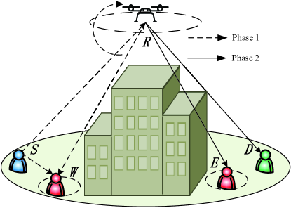
Figure 1: Delay-tolerant UAV relayed covert and secure communication model.

II-A System Model

As shown in Fig. 1, consider a delay-tolerant aerial relaying system with covertness and security high demand, where the direct link between the source (${S}$) and the destination (${D}$) is blocked, ${S}$ transmits the confidential data to ${D}$ with the help of an aerial relay (${R}$). At the same time, a terrestrial warden (${W}$) near ${S}$ tries to decide whether ${S}$ transmit or not and a terrestrial eavesdropper (${E}$) near ${D}$ wants to eavesdrop the confidential data sent by ${S}$ to ${D}$ through ${R}$’s relaying. In this system, all the terrestrial nodes are equipped with a single antenna. Assume that ${R}$ serves as a relay node within a period of $T$. The entire process is divided into two phases with durations of ${\alpha T}$ and ${\left({1-\alpha}\right)T}$ respectively, where $\alpha\in\left({0,1}\right)$ denotes the time switching factor between two phases. In the first phase, ${R}$, which equips a receive antenna and a transmit antenna and employs the decode-and-forward (DF) model, adopts the FD mode for receiving and jamming to ensure the covertness of the system. Subsequently, ${R}$ retransmit the confidential data to ${D}$ securely in the second phase. It is worth noting that in the first phase since ${R}$ is operating in the FD manner, self-interference cancellation (SIC) has to be applied. Nevertheless, since the SIC at ${R}$ cannot be canceled entirely in practice, the residual self-interference channel (RSIC) is considered in this work. Similar to [17], the RSIC ${{h_{RR}}}$ is modeled as Rayleigh fading channel, which means ${h_{RR}}\sim\mathcal{CN}\left({0,\psi}\right)$, where $\psi$ indicates the level of SIC.

For the concise and clear trajectory described, the duration of first phase ${\alpha T}$ is equally divided into ${N_{1}}$ time slots as ${\delta_{t,1}}=\frac{{\alpha T}}{{{N_{1}}}}$, and the duration of second phase ${\left({1-\alpha}\right)T}$ is equally divided into ${N_{2}}$ time slots as ${\delta_{t,2}}=\frac{{\left({1-\alpha}\right)T}}{{{N_{2}}}}$, when ${\delta_{t,k}},k\in\left\{{1,2}\right\}$ are small enough the position of ${R}$ is approximately fixed during each time slot [15]. Without loss of generality, all the nodes are described in the Cartesian coordinate system and the horizontal location of ${R}$ is denoted as ${{\bf{q}}_{R}}\left(n\right)={\left[{{x_{R}}\left(n\right),{y_{R}}\left(n\right)}\right]^{T}},n\in{\mathcal{N}}$, where ${\cal N}=\left\{{1,\cdots,N}\right\}$ and $N={N_{1}}+{N_{2}}$. For all the terrestrial nodes, their horizontal coordinates are expressed as ${{\bf{q}}_{S}}={\left[{{x_{S}},{y_{S}}}\right]^{T}}$, ${{\bf{q}}_{D}}={\left[{{x_{D}},{y_{D}}}\right]^{T}}$, ${{\bf{q}}_{W}}={\left[{{x_{W}},{y_{W}}}\right]^{T}}$ and ${{\bf{q}}_{E}}={\left[{{x_{E}},{y_{E}}}\right]^{T}}$, respectively. To guarantee the robustness of the communication system, the practical situation where the malicious nodes’ position is uncertain is assumed [26], [25]. According to this assumption, the positions of ${W}$ and ${E}$ are denoted as ${{\bf{q}}_{W}}={{\bf{\hat{q}}}_{W}}+\Delta{{\bf{q}}_{W}}$ and ${{\bf{q}}_{E}}={{\bf{\hat{q}}}_{E}}+\Delta{{\bf{q}}_{E}}$ respectively, where ${{\bf{\hat{q}}}_{j}}$, $j\in\left\{{W,E}\right\}$ are the estimated positions made by ${R}$-mounted cameras or radars [21], and $\Delta{{\bf{q}}_{j}}$ denote the estimation error follow ${\left\|{\Delta{{\bf{q}}_{j}}}\right\|^{2}}\leq r_{j}^{2}$, where $r_{j}$ are the estimation error degree for corresponding malicious node.

In this work, ${R}$ works at a fixed altitude $H$ and according to [3], the appropriate setting of the UAV flight height can make the LoS probability approximate to 1. Thus, it is assumed that the A2G links are LoS [14, 17]. Subsequently, the channel coefficients about ${R}$ in two phases are expressed as

$${h_{SR}}\left(n\right)=\sqrt{\frac{{{\beta_{0}}}}{{{{\left\|{{{\bf{q}}_{R}}\left(n\right)-{{\bf{q}}_{S}}}\right\|}^{2}}+{H^{2}}}}},$$ (1a)

$${h_{RW}}\left(n\right)=\sqrt{\frac{{{\beta_{0}}}}{{{{\left\|{{{\bf{q}}_{R}}\left(n\right)-{{\bf{q}}_{W}}}\right\|}^{2}}+{H^{2}}}}},$$ (1b)

and

$${h_{RD}}\left(n\right)=\sqrt{\frac{{{\beta_{0}}}}{{{{\left\|{{{\bf{q}}_{R}}\left(n\right)-{{\bf{q}}_{D}}}\right\|}^{2}}+{H^{2}}}}},$$ (2a)

$${h_{RE}}\left(n\right)=\sqrt{\frac{{{\beta_{0}}}}{{{{\left\|{{{\bf{q}}_{R}}\left(n\right)-{{\bf{q}}_{E}}}\right\|}^{2}}+{H^{2}}}}},$$ (2b)

respectively, where ${{\beta_{0}}}$ denotes the channel power gain at the reference distance. For ground-to-ground (G2G) link, the quasi-static Rayleigh model is utilized and the channel coefficient of $S$ to $W$ is expressed as

$${h_{SW}}=\sqrt{\frac{{{\beta_{0}}}}{{{{\left\|{{{\bf{q}}_{S}}-{{\bf{q}}_{W}}}\right\|}^{\eta}}}}}\zeta,$$ (3)

where $\zeta$ follows complex Gaussian distribution with zero mean and unit variance and $\eta>2$ means the path-loss exponent.

II-B Detection Performance

$$y_{W}^{i}\left(n\right)=\left\{{\begin{array}[]{*{20}{c}}{\sqrt{P_{R}^{J}}{h_{RW}}\left(n\right)x_{J}^{i}\left(n\right)+n_{W}^{i}\left(n\right)},&{{{\cal H}_{0}}}\\ {\sqrt{{P_{S}}\left(n\right)}{h_{SW}}x_{S}^{i}\left(n\right)+\sqrt{P_{R}^{J}}{h_{RW}}\left(n\right)x_{J}^{i}\left(n\right)+n_{W}^{i}\left(n\right)},&{{{\cal H}_{1}}}\end{array}}\right.$$ (4)

Similar to [24], assuming that $W$ conducts $I$ times monitoring actions in each time slot and sensing of the received signals to determine whether $S$ is transmitting or not. Then, for $W$, the binary hypothesis testing of the $i$-th $\left({i=1,\cdots,I}\right)$ received signal in the $n$th time slot is modeled as (4), shown at the top of next page, where ${{\mathcal{H}_{0}}}$ and ${{\mathcal{H}_{1}}}$ represent the hypothesis that $S$ is transmitting or not, ${{P_{S}}{\left(n\right)}}$ and ${P_{R}^{J}}$ represent the transmit power of $S$ and the jamming power of $R$ in the first phase, $x_{J}^{i}{\left(n\right)}$ and $x_{S}^{i}{\left(n\right)}$ are the transmitted signals following complex Gaussian distribution with zero mean and unit variance, and $n_{W}^{i}\left(n\right)$ is the complex additive Gaussian noise with power ${\sigma^{2}}$ at $W$.

The detection performance of $W$ is typically modeled by DEP in [19, 21, 22, 24, 26]. It is composed of false alarm probability (FAP) and miss detection probability (MDP), which are expressed as ${{\mathop{\rm P}\nolimits}_{{\rm{FA}}}}\left(n\right)=\Pr\left({{{\cal D}_{1}}|{{\cal H}_{0}}}\right)$ and ${{\mathop{\rm P}\nolimits}_{{\rm{MD}}}}\left(n\right)=\Pr\left({{{\cal D}_{0}}|{{\cal H}_{1}}}\right)$ respectively, where ${\mathcal{D}_{0}}$ and ${\mathcal{D}_{1}}$ represent the $W$’s decision biased towards to ${{\cal H}_{0}}$ and ${{\cal H}_{1}}$ respectively. To ensure covertness during the communication process, ${\xi_{W}}\left(n\right)\geq 1-\varepsilon$ should satisfied in the first phase, where ${\xi_{W}}\left(n\right)={{\mathop{\rm P}\nolimits}_{{\rm{FA}}}}\left(n\right)+{{\mathop{\rm P}\nolimits}_{{\rm{MD}}}}\left(n\right)$ and $0\leq\varepsilon\leq 1$ is an sufficiently small positive value which present the quality of covert service. Nevertheless, based on the results in [27, 28], there are incomplete Gamma functions in the expression of ${\xi_{W}}\left(n\right)$, which cause the subsequent analysis extremely intractable. To settle this difficulty, a tractable lower bound on ${\xi_{W}}\left(n\right)$ is built through Pinsker’s inequality [30], namely

$${\xi_{W}}\left(n\right)\geq 1-{{\mathbb{E}}_{\zeta}}\left({\sqrt{\frac{1}{2}{\mathcal{D}}\left({{\rm{P}}_{0}^{I}||{\rm{P}}_{1}^{I}}\right)}}\right),$$ (5)

where ${\rm{P}}_{0}^{I}=\prod\limits_{i=1}^{I}{f\left({y_{W}^{i}\left(n\right)|{{\cal H}_{0}}}\right)}$ and ${\rm{P}}_{1}^{I}=\prod\limits_{i=1}^{I}{f\left({y_{W}^{i}\left(n\right)|{{\cal H}_{1}}}\right)}$ are the likelihood functions under ${{\mathcal{H}_{0}}}$ and ${{\mathcal{H}_{1}}}$, respectively, $f\left({y_{W}^{i}\left(n\right)|{{\cal H}_{0}}}\right)=\mathcal{CN}\left({0,\sigma_{0}^{2}\left(n\right)}\right)$, $f\left({y_{W}^{i}\left(n\right)|{{\cal H}_{1}}}\right)=\mathcal{CN}\left({0,\sigma_{1}^{2}\left(n\right)}\right)$, $\sigma_{0}^{2}\left(n\right)=P_{R}^{J}{\left|{{h_{RW}}\left(n\right)}\right|^{2}}+{\sigma^{2}}$, $\sigma_{1}^{2}\left(n\right)={P_{S}}\left(n\right){\left|{{h_{SW}}}\right|^{2}}+P_{R}^{J}{\left|{{h_{RW}}\left(n\right)}\right|^{2}}+{\sigma^{2}}$, and ${\cal D}\left({{\rm{P}}_{0}^{I}||{\rm{P}}_{1}^{I}}\right)$ signifies the Kullback-Leibler (KL) divergence from ${{\rm{P}}_{0}^{I}}$ to ${{\rm{P}}_{1}^{I}}$, specifically represented as [24]

$${\cal D}\left({{\rm{P}}_{0}^{I}||{\rm{P}}_{1}^{I}}\right)=I\left({\ln\left({1+{\gamma_{W}}\left(n\right)}\right)-\frac{{{\gamma_{W}}\left(n\right)}}{{1+{\gamma_{W}}\left(n\right)}}}\right),$$ (6)

where ${\gamma_{W}}\left(n\right)=\frac{{{P_{S}}\left(n\right){{\left|{{h_{SW}}}\right|}^{2}}}}{{P_{R}^{J}{{\left|{{h_{RW}}\left(n\right)}\right|}^{2}}+{\sigma^{2}}}}$.

II-C Problem Formulation

According to the description in Section II-A and the DF protocol, the achievable rates in two phases are modeled as

$${R_{1}}\left(n\right) ={{\mathbb{E}}_{h_{RR}}}\left({B{{\log}_{2}}\left({1+\frac{{{P_{S}}\left(n\right){{\left|{{h_{SR}}\left(n\right)}\right|}^{2}}}}{{P_{R}^{J}{{\left|{{h_{RR}}}\right|}^{2}}+{\sigma^{2}}}}}\right)}\right)$$ (7)

$$\mathop{\geq}\limits^{\left(a\right)}B{\log_{2}}\left({1+\frac{{{P_{S}}\left(n\right){{\left|{{h_{SR}}\left(n\right)}\right|}^{2}}}}{{P_{R}^{J}\psi+{\sigma^{2}}}}}\right)\triangleq{R_{1}^{\sec}\left(n\right)},$$

and

$${R_{2}}\left(n\right)={\left[{{R_{D}}\left(n\right)-{R_{E}}\left(n\right)}\right]^{+}},$$ (8)

respectively, where ${\left[\cdot\right]^{+}}=\max\left({0,\cdot}\right)$, step $\left(a\right)$ is made by Jensen’s inequality [32], $B$ presents the channel bandwidth in hertz (Hz), ${R_{D}}\left(n\right)=B{\log_{2}}\left({1+\frac{{{P_{R}}\left(n\right){{\left|{{h_{RD}}\left(n\right)}\right|}^{2}}}}{{{\sigma^{2}}}}}\right)$ and ${R_{E}}\left(n\right)=B{\log_{2}}\left({1+\frac{{{P_{R}}\left(n\right){{\left|{{h_{RE}}\left(n\right)}\right|}^{2}}}}{{{\sigma^{2}}}}}\right)$. Then, the average achievable rate is stated as

$${R_{ave}}=\min\left({{\phi_{1}}\sum\limits_{n=1}^{{N_{1}}}{R_{1}^{\sec}\left(n\right)},{\phi_{2}}\sum\limits_{n={N_{1}}+1}^{N}{{R_{2}}\left(n\right)}}\right),$$ (9)

where ${\phi_{1}}=\frac{\alpha}{{{N_{1}}}}$, ${\phi_{2}}=\frac{{\left({1-\alpha}\right)}}{{{N_{2}}}}$. Nevertheless, due to the presentation of estimation error part in (9), the stochasticity of ${R_{ave}}$ needs to be attention. To deal with this issue, the triangle inequality is employed to obtain a lower bound of ${R_{ave}}$ which is shown as

$$\bar{R}_{ave}^{\sec}=\min\left({{\phi_{1}}\sum\limits_{n=1}^{{N_{1}}}{R_{1}^{\sec}\left(n\right)},{\phi_{2}}\sum\limits_{n={N_{1}}+1}^{N}{{{\left[{R_{2}^{\sec}\left(n\right)}\right]}^{+}}}}\right),$$ (10)

where

$$R_{2}^{\sec}\left(n\right)={{R_{D}}\left(n\right)-B{{\log}_{2}}\left({1+\frac{{{P_{R}}\left(n\right){{\left|{{{\hat{h}}_{RE}}\left(n\right)}\right|}^{2}}}}{{{\sigma^{2}}}}}\right)},$$ (11)

and ${\hat{h}_{RE}}\left(n\right)=\sqrt{\frac{{{\beta_{0}}}}{{{{\left({\left\|{{{\bf{q}}_{R}}\left(n\right)-{{{\bf{\hat{q}}}}_{E}}}\right\|-{r_{E}}}\right)}^{2}}+{H^{2}}}}}$ based on triangle inequality ${\hat{h}_{RE}}\left(n\right)\geq{h_{RE}}\left(n\right)$ is satisfied.

$${P_{C}}\left(n\right)={P_{0}}\left({1+\frac{{3{{\left\|{{{\bf{v}}_{R}}\left(n\right)}\right\|}^{2}}}}{{U_{tip}^{2}}}}\right)+{P_{1}}\sqrt{\left({\sqrt{1+\frac{{{{\left\|{{{\bf{v}}_{R}}\left(n\right)}\right\|}^{4}}}}{{4v_{0}^{4}}}}-\frac{{{{\left\|{{{\bf{v}}_{R}}\left(n\right)}\right\|}^{2}}}}{{2v_{0}^{2}}}}\right)}+\frac{1}{2}{d_{0}}\rho cS{\left\|{{{\bf{v}}_{R}}\left(n\right)}\right\|^{3}}$$ (12)

As derived in [29], for a rotary-wing UAV, the propulsion power is expressed as (12), shown at the top of this page, where ${P_{0}}$ and ${P_{1}}$ represent the blade profile and induced power in hovering status, respectively, ${U_{tip}}$ signifies the tip speed of the rotor blade, ${v_{0}}$ is the mean rotor induced velocity in hover, ${d_{0}}$, $\rho$, $c$ and $S$ are known as the fuselage drag ratio, air density, rotor solidity and rotor disc area, respectively, and ${{{\bf{v}}_{R}}\left(n\right)}$ expressed as

$${{\bf{v}}_{R}}\left(n\right)=\frac{1}{{{\delta_{t,k}}}}\left({{{\bf{q}}_{R}}\left(n\right)-{{\bf{q}}_{R}}\left({n-1}\right)}\right),n\in{{\mathcal{N}}_{k}},$$ (13)

where ${{\cal N}_{1}}=\left\{{1,\cdots,{N_{1}}}\right\}$ and ${{\cal N}_{2}}=\left\{{{N_{1}}+1,\cdots,N}\right\}$. When $\left|x\right|\ll 1$, via first-order Taylor approximation, $\sqrt{1+x}\approx 1+\frac{1}{2}x$ is satisfied. Similarly, when $\left\|{{{\bf{v}}_{R}}\left(n\right)}\right\|\gg{v_{0}}$, (12) is approximately transformed as

$$P_{C}^{\sec}\left(n\right)= {P_{0}}\left({1+\frac{{3{{\left\|{{{\bf{v}}_{R}}\left(n\right)}\right\|}^{2}}}}{{U_{tip}^{2}}}}\right)$$ (14)

$$+\frac{{{P_{1}}{v_{0}}}}{{\left\|{{{\bf{v}}_{R}}\left(n\right)}\right\|}}+\frac{1}{2}{d_{0}}\rho cS{\left\|{{{\bf{v}}_{R}}\left(n\right)}\right\|^{3}},$$

where the typical plot of the relationship between (12) and (14) is given by [29]. According to the Fig. 2 of [29], $P_{C}^{\sec}\left(n\right)\geq{P_{C}}\left(n\right)$ is satisfied. Additionally, the power utilized for transmission and jamming is much smaller than that for flight, so that can be neglected. Subsequently, a upper bound of the total energy consumption of $R$ in communication process is expressed as

$${E_{sum}}={\delta_{t,1}}\sum\limits_{n=1}^{{N_{1}}}{P_{C}^{\sec}\left(n\right)}+{\delta_{t,2}}\sum\limits_{n={N_{1}}+1}^{N}{P_{C}^{\sec}\left(n\right)}.$$ (15)

In this work, the energy efficient (EE) is defined as the ratio of average achievable rate and total energy consumption of $R$. Based on this definition, a tractable lower bound of EE of $R$ is formulated as

$$\varphi=\frac{{\bar{R}_{ave}^{\sec}}}{{{E_{sum}}}}.$$ (16)

Then a robust optimization problem for time switching factor $\alpha$, transmit power of transmitter ${{\bf{P}}_{S}}=\left\{{{P_{S}}\left(n\right),n\in{{\mathcal{N}}_{1}}}\right\}$, ${{\bf{P}}_{R,2}}=\left\{{{P_{R}}\left(n\right),n\in{{\mathcal{N}}_{2}}}\right\}$ and $R$’s trajectory ${{\bf{Q}}_{R}}=\left\{{{{\bf{q}}_{R}}\left(n\right),\forall n}\right\}$ is formulated as

$$\mathcal{P}_{1}:\; \mathop{\max}\limits_{{{\bf{P}}_{S}},{{\bf{P}}_{R,2}},{{\bf{Q}}_{R}},\alpha}\varphi$$ (17a)

$${\mathrm{s.t.}}\; 1-{{\mathbb{E}}_{\zeta}}\left({\sqrt{\frac{1}{2}{\cal D}\left({{\rm{P}}_{0}^{I}||{\rm{P}}_{1}^{I}}\right)}}\right)\geq 1-\varepsilon,n\in{{\mathcal{N}}_{1}},$$ (17b)

$$0\leq{P_{S}}\left(n\right)\leq{P_{S,\max}},n\in{{\mathcal{N}}_{1}},$$ (17c)

$$0\leq{P_{R}}\left(n\right)\leq{P_{R,\max}},n\in{{\mathcal{N}}_{2}},$$ (17d)

$${{\bf{q}}_{R}}\left(1\right)={{\bf{q}}^{I}},{{\bf{q}}_{R}}\left(N\right)={{\bf{q}}^{F}},$$ (17e)

$$\left\|{{{\bf{q}}_{R}}\left(n\right)-{{\bf{q}}_{R}}\left({n-1}\right)}\right\|\leq{\delta_{t,1}}{V_{\max}},n\in{{\mathcal{N}}_{1}},$$ (17f)

$$\left\|{{{\bf{q}}_{R}}\left(n\right)-{{\bf{q}}_{R}}\left({n-1}\right)}\right\|\leq{\delta_{t,2}}{V_{\max}},n\in{{\mathcal{N}}_{2}},$$ (17g)

$$\;0<\alpha<1,$$ (17h)

where (17b) is the covert constraint, (17c) and (17d) are the peak power constraint of $S$ in phase one and $R$ in phase two, respectively, where ${P_{S,\max}}$ and ${P_{R,\max}}$ signify the maximum transmit power, (17e) denotes the constraint on the take-off and landing position of $R$, ${{\bf{q}}^{I}}$ and ${{\bf{q}}^{F}}$ are the take-off and landing positions of $R$, respectively, (17f) and (17g) depict the maximum flight distance between adjacent time slots in phase one and phase two, respectively, and ${V_{\max}}$ denotes the maximum velocity of $R$.

III Problem Solution

Problem $\mathcal{P}_{1}$ is a multivariate coupled non-convex FP problem. As derived in [15], removing the operator ${\left[\cdot\right]^{+}}$ optimal value is also the same. Subsequently, using the Dinkelbach method [31], the original FP problem is transformed into the following problem to obtain the approximate solution, namely

$$\mathcal{P}_{2}:\; \mathop{\max}\limits_{{{\bf{P}}_{S}},{{\bf{P}}_{R,2}},{{\bf{Q}}_{R}},\alpha}R_{ave}^{\sec}-{\varphi^{\left(l\right)}}{E_{sum}}$$ (18a)

$${\mathrm{s.t.}}\; (\textrm{\ref{P1b}})-(\textrm{\ref{P1h}}),$$ (18b)

where ${\varphi^{\left(l\right)}}=\frac{{\bar{R}_{ave}^{\sec,\left(l\right)}}}{{E_{sum}^{\left(l\right)}}}$ is EE obtained in $l$-th iteration and $R_{ave}^{\sec}=\min\left({{\phi_{1}}\sum\limits_{n=1}^{{N_{1}}}{R_{1}^{\sec}\left(n\right)},{\phi_{2}}\sum\limits_{n={N_{1}}+1}^{N}{R_{2}^{\sec}\left(n\right)}}\right)$. Two factors in $\mathcal{P}_{2}$ must be noticed. One is the covert constraint (17b) is a non-convex constraint and there is not only the expected operation but also the position estimation error of $W$, the other is the non-concave objective function and it has highly complicated with respect to variable ${{\bf{P}}_{S}}$, ${{\bf{P}}_{R,2}}$, ${{\bf{Q}}_{R}}$ and $\alpha$. For the two challenges mentioned above, a lemma which provides a shrunken constraint and an AO-based algorithm is presented in the following subsection.

III-A Shrunken Covert Constraint

Lemma 1.

For (17b), a more stringent covertness constraint is given as $\bar{\gamma}_{W}^{\sec}\left(n\right)\leq{\gamma_{\max}},n=1,\cdots,{N_{1}}$, where $\bar{\gamma}_{W}^{\sec}\left(n\right)=\frac{{{P_{S}}\left(n\right){{\left|{\bar{h}_{SW}^{\sec}}\right|}^{2}}}}{{P_{R}^{J}{{\left|{h_{RW}^{\sec}\left(n\right)}\right|}^{2}}+{\sigma^{2}}}}$, $\bar{h}_{SW}^{\sec}=\sqrt{\frac{{{\beta_{0}}}}{{{{\left|{\left\|{{{\bf{q}}_{S}}-{{{\bf{\hat{q}}}}_{W}}}\right\|-{r_{W}}}\right|}^{\eta}}}}}$ and $h_{RW}^{\sec}\left(n\right)=\sqrt{\frac{{{\beta_{0}}}}{{{{\left({\left\|{{{\bf{q}}_{R}}\left(n\right)-{{{\bf{\hat{q}}}}_{W}}}\right\|+{r_{W}}}\right)}^{2}}+{H^{2}}}}}$.

Proof.

See Appendix A. ∎

By replacing (17b) into constraint mentioned by Lemma 1, problem $\mathcal{P}_{2}$ is rewritten as

$$\mathcal{P}_{3}:\; \mathop{\max}\limits_{{{\bf{P}}_{S}},{{\bf{P}}_{R,2}},{{\bf{Q}}_{R}},\alpha}R_{ave}^{\sec}-{\varphi^{\left(l\right)}}{E_{sum}}$$ (19a)

$${\mathrm{s.t.}}\; \bar{\gamma}_{W}^{\sec}\left(n\right)\leq{\gamma_{\max}},n\in{{\mathcal{N}}_{1}},$$ (19b)

$$(\textrm{\ref{P1c}})-(\textrm{\ref{P1h}}).$$ (19c)

III-B AO-Based Algorithm

In this subsection, an efficient AO-based algorithm is proposed to obtain a high-quality sub-optimal solution to problem $\mathcal{P}_{1}$. Specifically, problem $\mathcal{P}_{3}$ is tackled by alternately solving three sub-problems to optimize each of the time switching factor $\alpha$, the transmit power ${{\bf{P}}_{S}}$ and ${{\bf{P}}_{R,2}}$, and the $R$’s trajectory ${{\bf{Q}}_{R}}$.

1) Time Switching Factor: For fixed transmit power ${{\bf{P}}_{S}}$ and ${{\bf{P}}_{R,2}}$, and $R$’s trajectory ${{\bf{Q}}_{R}}$, problem $\mathcal{P}_{3}$ is reduced to

$$\mathcal{P}_{3.1.1}:\; \mathop{\max}\limits_{\alpha}R_{ave}^{\sec}-{\varphi^{\left(l\right)}}{E_{sum}}$$ (20a)

$${\mathrm{s.t.}}\; (\textrm{\ref{P1f}})-(\textrm{\ref{P1h}}),$$ (20b)

which is a non-convex optimization problem. By introducing the slack variable ${\omega_{1}}$, a equivalent form of $\mathcal{P}_{3.1.1}$ is obtained as

$$\mathcal{P}_{3.1.2}:\; \mathop{\max}\limits_{\alpha,{\omega_{1}}}\;{\omega_{1}}-{\varphi^{\left(l\right)}}{E_{sum}}$$ (21a)

$${\mathrm{s.t.}}\; -{\omega_{1}}+\alpha{\rho_{1}}\geq 0,$$ (21b)

$$-{\omega_{1}}+\left({1-\alpha}\right){\rho_{2}}\geq 0,$$ (21c)

$$\;\alpha-{\beta_{1}}\geq 0,$$ (21d)

$$-\alpha-{\beta_{2}}+1\geq 0,$$ (21e)

which is a standard convex optimization problem that satisfies Slater’s condition, where ${\rho_{1}}=\frac{1}{{{N_{1}}}}\sum\limits_{n=1}^{{N_{1}}}{R_{1}^{\sec}\left(n\right)}$, ${\rho_{2}}=\frac{1}{{{N_{2}}}}\sum\limits_{n={N_{1}}+1}^{N}{R_{2}^{\sec}\left(n\right)}$, and ${\beta_{k}}=\frac{{{N_{k}}\mathop{\max}\limits_{n\in{{\mathcal{N}}_{k}}}\left\|{{{\bf{q}}_{R}}\left(n\right)-{{\bf{q}}_{R}}\left({n-1}\right)}\right\|}}{{T{V_{\max}}}}$.

The KKT conditions of $\mathcal{P}_{3.1.2}$ is formed as

$$-{\varphi^{\left(l\right)}}\frac{{d{E_{sum}}\left({{\alpha^{*}}}\right)}}{{d\alpha}}+\lambda_{1}^{*}{\rho_{1}}-\lambda_{2}^{*}{\rho_{2}}+\lambda_{3}^{*}-\lambda_{4}^{*}=0,$$ (22a)

$$1-\lambda_{1}^{*}-\lambda_{2}^{*}=0,\lambda_{1}^{*}\geq 0,\lambda_{2}^{*}\geq 0,\lambda_{3}^{*}\geq 0,\lambda_{4}^{*}\geq 0,$$ (22b)

$$\lambda_{1}^{*}\left({-\omega_{1}^{*}+{\alpha^{*}}{\rho_{1}}}\right)=0,\lambda_{2}^{*}\left({-\omega_{1}^{*}+\left({1-{\alpha^{*}}}\right){\rho_{2}}}\right)=0,$$ (22c)

$$\lambda_{3}^{*}\left({{\alpha^{*}}-{\beta_{1}}}\right)=0,\lambda_{4}^{*}\left({-{\alpha^{*}}-{\beta_{2}}+1}\right)=0,$$ (22d)

$$-\omega_{1}^{*}+{\alpha^{*}}{\rho_{1}}\geq 0,-\omega_{1}^{*}+\left({1-{\alpha^{*}}}\right){\rho_{2}}\geq 0,$$ (22e)

$${\alpha^{*}}-{\beta_{1}}\geq 0,-{\alpha^{*}}-{\beta_{2}}+1\geq 0,$$ (22f)

where $\lambda_{1}^{*}$, $\lambda_{2}^{*}$, $\lambda_{3}^{*}$ and $\lambda_{4}^{*}$ are the Lagrange multipliers. It is challenging to derive an analytical expression for ${\alpha^{*}}$ directly from the above conditions so a novel algorithm based on the primal-dual search method, PDSA, is proposed, and the derivation details are shown as follows.

By substituting (22b) into (22a), the stationarity condition is equally transformed into

$$-{\varphi^{\left(l\right)}}\frac{{d{E_{sum}}\left({{\alpha^{*}}}\right)}}{{d\alpha}}+{\rho_{1}}-\lambda_{2}^{*}\left({{\rho_{1}}+{\rho_{2}}}\right)+\lambda_{3}^{*}-\lambda_{4}^{*}=0.$$ (23)

To search the optimal value ${\alpha^{*}}$, several following factors should be noticed:

1. Since ${{E_{sum}}\left({{\alpha}}\right)}$ is convex function with respect to ${\alpha}$, it is not difficult to know that $\frac{{d{E_{sum}}\left({{\alpha}}\right)}}{{d\alpha}}$ is monotonically increasing with respect to ${\alpha}$.

2. The ${\hat{\alpha}_{1}}$ which meets $-{\varphi^{\left(l\right)}}\frac{{d{E_{sum}}\left({{{\hat{\alpha}}_{1}}}\right)}}{{d\alpha}}+{\rho_{1}}=0$ can be obtained by bisection search method.

3. The ${\hat{\alpha}_{2}}$ calculated by ${\hat{\alpha}_{2}}{\rho_{1}}=\left({1-{{\hat{\alpha}}_{2}}}\right){\rho_{2}}$.

4. The ${\hat{\alpha}_{3}}$ which meets $-{\varphi^{\left(l\right)}}\frac{{d{E_{sum}}\left({\hat{\alpha}_{3}}\right)}}{{d\alpha}}-{\rho_{2}}=0$ calculated by bisection search method.

5. Based on a), b) and d), ${\hat{\alpha}_{1}}>{\hat{\alpha}_{3}}$ is satisfied.

6. According to the function of $\mathcal{P}_{3.1.2}$, it is known that if the feasibility conditions (22e) are met, a larger value of $\omega_{1}^{*}$ is considered better.

When ${\hat{\alpha}_{1}}\in\left({{\beta_{1}},1-{\beta_{2}}}\right)$:

1. If ${\hat{\alpha}_{1}}{\rho_{1}}\leq\left({1-{{\hat{\alpha}}_{1}}}\right){\rho_{2}}$ is satisfied, ${\hat{\alpha}_{1}}$ is the optimal value of $\alpha$. This is because when ${\alpha^{*}}={\hat{\alpha}_{1}}$, the corresponding solutions $\omega_{1}^{*}$, $\lambda_{1}^{*}$, $\lambda_{2}^{*}$, $\lambda_{3}^{*}$ and $\lambda_{4}^{*}$ that satisfy conditions (22) can be found.

2. When ${\hat{\alpha}_{1}}{\rho_{1}}>\left({1-{{\hat{\alpha}}_{1}}}\right){\rho_{2}}$, if ${\hat{\alpha}_{2}}\in\left({{\beta_{1}},{{\hat{\alpha}}_{1}}}\right)$ and ${\hat{\alpha}_{2}}\geq{\hat{\alpha}_{3}}$ are satisfied, ${\hat{\alpha}_{2}}$ is the optimal value of $\alpha$. This is due to in this situation, based on a) - d), it is known that ${\hat{\alpha}_{2}}<{\hat{\alpha}_{1}}$, ${\hat{\alpha}_{2}}{\rho_{1}}=\left({1-{{\hat{\alpha}}_{2}}}\right){\rho_{2}}$, $-{\varphi^{\left(l\right)}}\frac{{d{E_{sum}}\left({{{\hat{\alpha}}_{2}}}\right)}}{{d\alpha}}+{\rho_{1}}>0$ and $-{\varphi^{\left(l\right)}}\frac{{d{E_{sum}}\left({\hat{\alpha}_{2}}\right)}}{{d\alpha}}-{\rho_{2}}\leq 0$ are satisfied. Based on the above and (22b) - (22f), when ${\alpha^{*}}={\hat{\alpha}_{2}}$, $1\geq\lambda_{1}^{*}\geq 0$, $1\geq\lambda_{2}^{*}\geq 0$, $\lambda_{3}^{*}=0$ and $\lambda_{4}^{*}=0$ are satisfied. Finally, the $\lambda_{1}^{*}$, $\lambda_{2}^{*}$, $\lambda_{3}^{*}$ and $\lambda_{4}^{*}$ corresponding to ${\alpha^{*}}={\hat{\alpha}_{2}}$ can be found to satisfy (23).

3. When ${\hat{\alpha}_{1}}{\rho_{1}}>\left({1-{{\hat{\alpha}}_{1}}}\right){\rho_{2}}$ and ${\hat{\alpha}_{2}}\in\left({{\beta_{1}},{{\hat{\alpha}}_{1}}}\right)$, if ${\hat{\alpha}_{3}}>{\hat{\alpha}_{2}}$ is satisfied, ${\hat{\alpha}_{3}}$ is the optimal value of $\alpha$. The reason why ${\alpha^{*}}={\hat{\alpha}_{3}}$ is that in this situation, according to c) - e), ${\hat{\alpha}_{3}}{\rho_{1}}>\left({1-{{\hat{\alpha}}_{3}}}\right){\rho_{2}}$, $-{\varphi^{\left(l\right)}}\frac{{d{E_{sum}}\left({\hat{\alpha}_{3}}\right)}}{{d\alpha}}-{\rho_{2}}=0$ and ${\hat{\alpha}_{1}}>{\hat{\alpha}_{3}}$ are satisfied. Based on the above and (22b) - (22f), when ${\alpha^{*}}={\hat{\alpha}_{3}}$, it is known that $\lambda_{1}^{*}=0$, $\lambda_{2}^{*}=1$, $\lambda_{3}^{*}=0$ and $\lambda_{4}^{*}=0$, and (23) is satisfied.

4. When ${\hat{\alpha}_{1}}{\rho_{1}}>\left({1-{{\hat{\alpha}}_{1}}}\right){\rho_{2}}$ and ${\hat{\alpha}_{2}}\notin\left({{\beta_{1}},{{\hat{\alpha}}_{1}}}\right)$, if ${\beta_{1}}\geq{\hat{\alpha}_{3}}$ is satisfied, $\beta_{1}$ is the optimal value of $\alpha$. This is because in this situation, according to c) and d), ${\beta_{1}}\geq{\hat{\alpha}_{2}}$, ${\beta_{1}}{\rho_{1}}\geq\left({1-{\beta_{1}}}\right){\rho_{2}}$ and $-{\varphi^{\left(l\right)}}\frac{{d{E_{sum}}\left({{\beta_{1}}}\right)}}{{d\alpha}}-{\rho_{2}}\leq 0$ are satisfied. Based on the above and (22b) - (22f), when ${\alpha^{*}}={\beta_{1}}$, it is known that $\lambda_{1}^{*}=0$, $\lambda_{2}^{*}=1$, $\lambda_{3}^{*}\geq 0$ and $\lambda_{4}^{*}=0$, and (23) is satisfied.

5. When ${\hat{\alpha}_{1}}{\rho_{1}}>\left({1-{{\hat{\alpha}}_{1}}}\right){\rho_{2}}$ and ${\hat{\alpha}_{2}}\notin\left({{\beta_{1}},{{\hat{\alpha}}_{1}}}\right)$, if ${\beta_{1}}<{\hat{\alpha}_{3}}$, which indicates ${\hat{\alpha}_{3}}>{\hat{\alpha}_{2}}$, similar to iii), ${\hat{\alpha}_{3}}$ is the optimal value of $\alpha$.

When ${\hat{\alpha}_{1}}\notin\left({{\beta_{1}},1-{\beta_{2}}}\right)$, the optimal value ${\alpha^{*}}$ can be searched by similar way to the case of ${\hat{\alpha}_{1}}\in\left({{\beta_{1}},1-{\beta_{2}}}\right)$.

According to the above, the proposed PDSA algorithm that efficiently solves problem $\mathcal{P}_{3.1.2}$ is summarized in Algorithm 1.

Calculate ${\beta_{1}}$, ${\beta_{2}}$, ${\rho_{1}}$, ${\rho_{2}}$, ${\hat{\alpha}_{1}}$, ${\hat{\alpha}_{2}}$ and ${\hat{\alpha}_{3}}$, respectively;

if ${\hat{\alpha}_{1}}\in\left({{\beta_{1}},1-{\beta_{2}}}\right)$ then

       if ${\hat{\alpha}_{1}}{\rho_{1}}\leq\left({1-{{\hat{\alpha}}_{1}}}\right){\rho_{2}}$ then

            ${\alpha^{*}}={\hat{\alpha}_{1}}$.

      else

             if ${\hat{\alpha}_{2}}\in\left({{\beta_{1}},{{\hat{\alpha}}_{1}}}\right)$ then

                   if ${\hat{\alpha}_{2}}\geq{\hat{\alpha}_{3}}$ then

                        ${\alpha^{*}}={\hat{\alpha}_{2}}$.

                  else

                        ${\alpha^{*}}={\hat{\alpha}_{3}}$.

                   end if

                  

            else

                   if ${\beta_{1}}\geq{\hat{\alpha}_{3}}$ then

                        ${\alpha^{*}}={\beta_{1}}$.

                  else

                        ${\alpha^{*}}={\hat{\alpha}_{3}}$.

                   end if

                  

             end if

            

       end if

      

else

       if ${\hat{\alpha}_{1}}\leq{\beta_{1}}$ then

            ${\alpha^{*}}={\beta_{1}}$.

      else

             if $\left({1-{\beta_{2}}}\right){\rho_{1}}\leq{\beta_{2}}{\rho_{2}}$ then

                  ${\alpha^{*}}=1-{\beta_{2}}$.

            else

                   if ${\hat{\alpha}_{2}}\in\left[{{\beta_{1}},1-{\beta_{2}}}\right)$ then

                         if ${\hat{\alpha}_{2}}\geq{\hat{\alpha}_{3}}$ then

                              ${\alpha^{*}}={\hat{\alpha}_{2}}$.

                        else

                              ${\alpha^{*}}={\hat{\alpha}_{3}}$.

                         end if

                        

                  else

                         if ${\beta_{1}}\geq{\hat{\alpha}_{3}}$ then

                              ${\alpha^{*}}={\beta_{1}}$.

                        else

                               if ${\hat{\alpha}_{3}}\leq{1-{\beta_{2}}}$ then

                                    ${\alpha^{*}}={\hat{\alpha}_{3}}$.

                              else

                                    ${\alpha^{*}}={1-{\beta_{2}}}$.

                               end if

                              

                         end if

                        

                   end if

                  

             end if

            

       end if

      

end if

Output: ${\alpha^{*}}$.

Algorithm 1 Primal-Dual Search Based Algorithm

2) Transmit Power: For the sub-problem for given ${{\bf{Q}}_{R}}$ and $\alpha$, the objective function is non-convex with respect to ${{\bf{P}}_{S}}$ and ${{\bf{P}}_{R,2}}$. By introducing the slack variable ${\omega_{2}}$, the following equivalent problem is formed as

$$\mathcal{P}_{3.2.1}:\; \mathop{\max}\limits_{{{\bf{P}}_{S}},{{\bf{P}}_{R,2}},{\omega_{2}}}{\omega_{2}}-{\varphi^{\left(l\right)}}{E_{sum}}$$ (24a)

$${\mathrm{s.t.}}\; {\phi_{1}}\sum\limits_{n=1}^{{N_{1}}}{R_{1}^{\sec}\left(n\right)}\geq{\omega_{2}},$$ (24b)

$${\phi_{2}}\sum\limits_{n={N_{1}}+1}^{N}{R_{2}^{\sec}\left(n\right)}\geq{\omega_{2}},$$ (24c)

$$(\textrm{\ref{P3b}}),(\textrm{\ref{P1c}}),(\textrm{\ref{P1d}}).$$ (24d)

$$B{\log_{2}}\left({{\sigma^{2}}+{P_{R}}\left(n\right){{\left|{{{\hat{h}}_{RE}}\left(n\right)}\right|}^{2}}}\right)\leq\underbrace{B{{\log}_{2}}\left({{\sigma^{2}}+P_{R}^{\left(l\right)}\left(n\right){{\left|{{{\hat{h}}_{RE}}\left(n\right)}\right|}^{2}}}\right)+\frac{{B{{\left|{{{\hat{h}}_{RE}}\left(n\right)}\right|}^{2}}\left({{P_{R}}\left(n\right)-P_{R}^{\left(l\right)}\left(n\right)}\right)}}{{\left({{\sigma^{2}}+P_{R}^{\left(l\right)}\left(n\right){{\left|{{{\hat{h}}_{RE}}\left(n\right)}\right|}^{2}}}\right)\ln\left(2\right)}}}_{\buildrel\Delta\over{=}K\left(n\right)}$$ (25)

Despite the non-convexity still present in (24c), an approximate convex form can be formed by SCA method, namely (25), shown at the top of next page, where $\left\{{P_{R}^{\left(l\right)}\left(n\right),n\in{{\mathcal{N}}_{2}}}\right\}$ is fixed obtained by Algorithm 2 in the $l$-th iteration. By replacing the corresponding part of constraint (24c) with the approximate form, an approximate convex problem of $\mathcal{P}_{3.2.1}$ which can be solved by CVX toolbox is modeled as [32]

$$\mathcal{P}_{3.2.2}:\; \mathop{\max}\limits_{{{\bf{P}}_{S}},{{\bf{P}}_{R,2}},{\omega_{2}}}{\omega_{2}}-{\varphi^{\left(l\right)}}{E_{sum}}$$ (26a)

$${\mathrm{s.t.}}\; {\phi_{2}}\sum\limits_{n={N_{1}}+1}^{N}{\left({R_{D}^{\sec}\left(n\right)-K\left(n\right)}\right)}\geq{\omega_{2}},$$ (26b)

$$(\textrm{\ref{P3.2.1b}}),(\textrm{\ref{P3.2.1d}}),$$ (26c)

where $R_{D}^{\sec}\left(n\right)=B{\log_{2}}\left({{\sigma^{2}}+{P_{R}}\left(n\right){{\left|{{h_{RD}}\left(n\right)}\right|}^{2}}}\right)$.

3) Trajectory of $R$: By reducing problem $\mathcal{P}_{3}$, the sub-problem with respect to ${{{\bf{Q}}_{R}}}$ is expressed as

$$\mathcal{P}_{3.3.1}:\; \mathop{\max}\limits_{{{\bf{Q}}_{R}}}R_{ave}^{\sec}-{\varphi^{\left(l\right)}}{E_{sum}}$$ (27a)

$${\mathrm{s.t.}}\; \bar{\gamma}_{W}^{\sec}\left(n\right)\leq{\gamma_{\max}},n\in{{\mathcal{N}}_{1}},$$ (27b)

$$(\textrm{\ref{P1e}})-(\textrm{\ref{P1g}}).$$ (27c)

Even with given ${{\bf{P}}_{S}}$, ${{\bf{P}}_{R,2}}$ and ${\alpha}$, problem $\mathcal{P}_{3.3.1}$ is still intractable to solve optimally since the non-convexity and the strong coupling regarding ${{\bf{Q}}_{R}}$ still exist in objective function and constraint (27b). To tackle the strong coupling with respect to ${{\bf{Q}}_{R}}$, the slack variables ${\omega_{3}}$, $\lambda=\left\{{\lambda\left(n\right),n\in{\mathcal{N}}}\right\}$, $\nu=\left\{{\nu\left(n\right),n\in{{\mathcal{N}}_{1}}}\right\}$, $\kappa=\left\{{\kappa\left(n\right),n\in{{\mathcal{N}}_{2}}}\right\}$, $\varpi=\left\{{\varpi\left(n\right),n\in{{\mathcal{N}}_{2}}}\right\}$ and $\vartheta=\left\{{\vartheta\left(n\right),n\in{{\mathcal{N}}_{1}}}\right\}$ is introduced to obtain a equivalent form of problem $\mathcal{P}_{3.3.1}$, which is expressed as

$$\mathcal{P}_{3.3.2}:\; \mathop{\max}\limits_{{{\bf{Q}}_{R}},{\omega_{3}},\lambda,\nu,\kappa,\varpi,\vartheta}{\omega_{3}}-{\varphi^{\left(l\right)}}E_{sum}^{\sec}$$ (28a)

$${\mathrm{s.t.}}\; {\lambda^{2}}\left(n\right)\leq{\left\|{{{\bf{q}}_{R}}\left(n\right)-{{\bf{q}}_{R}}\left({n-1}\right)}\right\|^{2}},n\in{\mathcal{N}},$$ (28b)

$${{\phi}_{1}}\sum\limits_{n=1}^{{N_{1}}}{R_{1}^{\sec,1}\left(n\right)}\geq{\omega_{3}},$$ (28c)

$${\phi_{2}}\sum\limits_{n={N_{1}}+1}^{N}{R_{2}^{\sec,1}\left(n\right)}\geq{\omega_{3}},$$ (28d)

$${P_{S}}\left(n\right){\left|{\bar{h}_{SW}^{\sec}}\right|^{2}}\leq\frac{{{\gamma_{\max}}{\beta_{0}}P_{R}^{J}}}{{\vartheta\left(n\right)}}+{\gamma_{\max}}{\sigma^{2}},n\in{{\mathcal{N}}_{1}},$$ (28e)

$$\nu\left(n\right)\geq{\left\|{{{\bf{q}}_{R}}\left(n\right)-{{\bf{q}}_{S}}}\right\|^{2}}+{H^{2}},n\in{{\mathcal{N}}_{1}},$$ (28f)

$$\kappa\left(n\right)\geq{\left\|{{{\bf{q}}_{R}}\left(n\right)-{{\bf{q}}_{D}}}\right\|^{2}}+{H^{2}},n\in{{\mathcal{N}}_{2}},$$ (28g)

$$\varpi\left(n\right)\leq{\left({\left\|{{{\bf{q}}_{R}}\left(n\right)-{{{\bf{\hat{q}}}}_{E}}}\right\|-{r_{E}}}\right)^{2}}+{H^{2}},n\in{{\mathcal{N}}_{2}},$$ (28h)

$$\vartheta\left(n\right)\geq{\left({\left\|{{{\bf{q}}_{R}}\left(n\right)-{{{\bf{\hat{q}}}}_{W}}}\right\|+{r_{W}}}\right)^{2}}+{H^{2}},n\in{{\mathcal{N}}_{1}},$$ (28i)

$$(\textrm{\ref{P1e}})-(\textrm{\ref{P1g}}),$$ (28j)

where $E_{sum}^{\sec}$ is given in (29), shown at the top of next page, $R_{1}^{\sec,1}\left(n\right)=B{\log_{2}}\left({1+\frac{{{P_{S}}\left(n\right){\beta_{0}}}}{{\nu\left(n\right)\left({P_{R}^{J}\psi+{\sigma^{2}}}\right)}}}\right)$, $R_{2}^{\sec,1}\left(n\right)=R_{D}^{\sec,1}\left(n\right)-R_{E}^{\sec,1}\left(n\right)$, $R_{D}^{\sec,1}\left(n\right)=B{\log_{2}}\left({1+\frac{{{P_{R}}\left(n\right){\beta_{0}}}}{{\kappa\left(n\right){\sigma^{2}}}}}\right)$ and $R_{E}^{\sec,1}\left(n\right)=B{\log_{2}}\left({1+\frac{{{P_{R}}\left(n\right){\beta_{0}}}}{{\varpi\left(n\right){\sigma^{2}}}}}\right)$.

$$E_{sum}^{\sec} ={\delta_{t,1}}\sum\limits_{n=1}^{{N_{1}}}{\left({{P_{0}}\left({1+\frac{{3{{\left\|{{{\bf{v}}_{R}}\left(n\right)}\right\|}^{2}}}}{{U_{tip}^{2}}}}\right)+\frac{{{\delta_{t,1}}{P_{1}}{v_{0}}}}{{\lambda\left(n\right)}}+\frac{1}{2}{d_{0}}\rho sA{{\left\|{{{\bf{v}}_{R}}\left(n\right)}\right\|}^{3}}}\right)}$$ (29)

$$+{\delta_{t,2}}\sum\limits_{n={N_{1}}+1}^{N-1}{\left({{P_{0}}\left({1+\frac{{3{{\left\|{{{\bf{v}}_{R}}\left(n\right)}\right\|}^{2}}}}{{U_{tip}^{2}}}}\right)+\frac{{{\delta_{t,2}}{P_{1}}{v_{0}}}}{{\lambda\left(n\right)}}+\frac{1}{2}{d_{0}}\rho sA{{\left\|{{{\bf{v}}_{R}}\left(n\right)}\right\|}^{3}}}\right)}$$

Subsequently, to handle the residual non-convexity, the first-order Taylor expansion is applied to build an approximate convex problem which can be efficiently solved by CVX toolbox [32], namely

$$\mathcal{P}_{3.3.3}:\; \mathop{\max}\limits_{{{\bf{Q}}_{R}},{\omega_{3}},\lambda,\nu,\kappa,\varpi,\vartheta}{\omega_{3}}-{\varphi^{\left(l\right)}}E_{sum}^{\sec}$$ (30a)

$${\mathrm{s.t.}}\; {\lambda^{2}}\left(n\right)\leq B\left(n\right),n\in{\mathcal{N}},$$ (30b)

$${{\phi}_{1}}\sum\limits_{n=1}^{{N_{1}}}{\left({R_{1}^{\sec,2}\left(n\right)-C\left(n\right)}\right)}\geq{\omega_{3}},$$ (30c)

$${{\phi}_{2}}\sum\limits_{n={N_{1}}+1}^{N}{\left({R_{2}^{\sec,2}\left(n\right)-D\left(n\right)-E\left(n\right)}\right)}\geq{\omega_{3}},$$ (30d)

$$\varpi\left(n\right)\leq F\left(n\right)+{H^{2}},n\in{{\mathcal{N}}_{2}},$$ (30e)

$$(\textrm{\ref{P3.3.2e}}),(\textrm{\ref{P3.3.2f}}),(\textrm{\ref{P3.3.2g}}),(\textrm{\ref{P3.3.2i}}),(\textrm{\ref{P3.3.2j}}),$$ (30f)

where $R_{1}^{\sec,2}\left(n\right)=B{\log_{2}}\left({\nu\left(n\right)\left({P_{R}^{J}\psi+{\sigma^{2}}}\right)+{P_{S}}\left(n\right){\beta_{0}}}\right)$, $R_{2}^{\sec,2}\left(n\right)=B{\log_{2}}\left({\kappa\left(n\right){\sigma^{2}}+{P_{R}}\left(n\right){\beta_{0}}}\right)+{\log_{2}}\left({\varpi\left(n\right){\sigma^{2}}}\right)$ and $B\left(n\right),\cdots,F\left(n\right)$ are presented as (31), shown at the top of this page, where $\left\{{{\bf{q}}_{R}^{\left(l\right)}\left(n\right),n\in{\mathcal{N}}}\right\}$, $\left\{{{\nu^{\left(l\right)}}\left(n\right),n\in{{\mathcal{N}}_{1}}}\right\}$, $\left\{{{\kappa^{\left(l\right)}}\left(n\right),n\in{{\mathcal{N}}_{2}}}\right\}$ and $\left\{{{\varpi^{\left(l\right)}}\left(n\right),n\in{{\mathcal{N}}_{2}}}\right\}$ are obtained by Algorithm 2 in $l$-th iteration.

$$B\left(n\right)={\left\|{{\bf{q}}_{R}^{\left(l\right)}\left(n\right)-{\bf{q}}_{R}^{\left(l\right)}\left({n-1}\right)}\right\|^{2}}+2{\left({{\bf{q}}_{R}^{\left(l\right)}\left(n\right)-{\bf{q}}_{R}^{\left(l\right)}\left({n-1}\right)}\right)^{T}}\left({{{\bf{q}}_{R}}\left(n\right)-{{\bf{q}}_{R}}\left({n-1}\right)-{\bf{q}}_{R}^{\left(l\right)}\left(n\right)+{\bf{q}}_{R}^{\left(l\right)}\left({n-1}\right)}\right)$$ (31a)

$$C\left(n\right)=B{\log_{2}}\left({{\nu^{\left(l\right)}}\left(n\right)\left({P_{R}^{J}\psi+{\sigma^{2}}}\right)}\right)+\frac{B}{{{\nu^{\left(l\right)}}\left(n\right)\ln\left(2\right)}}\left({\nu\left(n\right)-{\nu^{\left(l\right)}}\left(n\right)}\right)$$ (31b)

$$D\left(n\right)=B{\log_{2}}\left({{\kappa^{\left(l\right)}}\left(n\right){\sigma^{2}}}\right)+\frac{B}{{{\kappa^{\left(l\right)}}\left(n\right)\ln\left(2\right)}}\left({\kappa\left(n\right)-{\kappa^{\left(l\right)}}\left(n\right)}\right)$$ (31c)

$$E\left(n\right)=B{\log_{2}}\left({{\varpi^{\left(l\right)}}\left(n\right){\sigma^{2}}+{P_{R}}\left(n\right){\beta_{0}}}\right)+\frac{{\left({\varpi\left(n\right)-{\varpi^{\left(l\right)}}\left(n\right)}\right)B{\sigma^{2}}}}{{\left({{\varpi^{\left(l\right)}}\left(n\right){\sigma^{2}}+P_{R}^{\left(l\right)}\left(n\right){\beta_{0}}}\right)\ln\left(2\right)}}$$ (31d)

$$F\left(n\right)={\left({\left\|{{\bf{q}}_{R}^{\left(l\right)}\left(n\right)-{{{\bf{\hat{q}}}}_{E}}}\right\|-{r_{E}}}\right)^{2}}+\frac{2{\left({\left\|{{\bf{q}}_{R}^{\left(l\right)}\left(n\right)-{{{\bf{\hat{q}}}}_{E}}}\right\|-{r_{E}}}\right)}}{{\left\|{{\bf{q}}_{R}^{\left(l\right)}\left(n\right)-{{{\bf{\hat{q}}}}_{E}}}\right\|}}{\left({{\bf{q}}_{R}^{\left(l\right)}\left(n\right)-{{{\bf{\hat{q}}}}_{E}}}\right)^{T}}\left({{{\bf{q}}_{R}}\left(n\right)-{\bf{q}}_{R}^{\left(l\right)}\left(n\right)}\right)$$ (31e)

Finally, the AO-based algorithm which is summarized in Algorithm 2 is developed to solve problem $\mathcal{P}_{1}$ sub-optimally, where $\hat{\xi}$ present the accuracy of convergence.

Input: Initialize ${\bf{P}}_{S}^{\left(0\right)}$, ${\bf{P}}_{R,2}^{\left(0\right)}$, ${\bf{Q}}_{R}^{\left(0\right)}$ and ${\alpha^{\left(0\right)}}$. Calculate ${\varphi^{\left(0\right)}}$ and $l\leftarrow 0$;

do

       Solve $\mathcal{P}_{3.1.2}$ by Algorithm 1 with given ${\bf{P}}_{S}^{\left(l\right)}$, ${\bf{P}}_{R,2}^{\left(l\right)}$ and ${\bf{Q}}_{R}^{\left(l\right)}$;

       Solve $\mathcal{P}_{3.2.2}$ with given ${\bf{Q}}_{R}^{\left(l\right)}$ and ${\alpha^{\left(l+1\right)}}$;

       Solve $\mathcal{P}_{3.3.3}$ with given ${\bf{P}}_{S}^{\left({l+1}\right)}$, ${\bf{P}}_{R,2}^{\left({l+1}\right)}$ and ${\alpha^{\left({l+1}\right)}}$;

       $l\leftarrow l+1$;

       Calculate the EE value ${\varphi^{\left(l\right)}}$;

while ${\varphi^{\left(l\right)}}-{\varphi^{\left({l-1}\right)}}>\hat{\xi}$;

Output: ${\varphi^{\left(l\right)}}$ with ${\bf{P}}_{S}^{*}={\bf{P}}_{S}^{\left(l\right)}$, ${\bf{P}}_{R,2}^{*}={\bf{P}}_{R,2}^{\left(l\right)}$, ${\bf{Q}}_{R}^{*}={\bf{Q}}_{R}^{\left(l\right)}$, ${\alpha^{*}}={\alpha^{\left(l\right)}}$.

Algorithm 2 Proposed AO-Based Algorithm for Non-Convex Problem $\mathcal{P}_{1}$

III-C Convergence and Complexity Analysis

In this subsection, based on the results presented in the previous, the convergence of Algorithm 2 is proved as follows.

Proof.

Suppose $\varphi\left({{\bf{P}}_{S}^{\left({l-1}\right)},{\bf{P}}_{R,2}^{\left({l-1}\right)},{\bf{Q}}_{R}^{\left({l-1}\right)},{\alpha^{\left({l-1}\right)}}}\right)$ indicates the objective value of the problem $\mathcal{P}_{1}$ in $\left(l-1\right)$-th iteration. First, due to the optimal value of problem $\mathcal{P}_{3.1.1}$ is obtained to solve equivalent form $\mathcal{P}_{3.1.2}$ via PDSA, then have

$$\varphi\left({{\bf{P}}_{S}^{\left({l-1}\right)},{\bf{P}}_{R,2}^{\left({l-1}\right)},{\bf{Q}}_{R}^{\left({l-1}\right)},{\alpha^{\left({l-1}\right)}}}\right)$$ (32)

$$\;\;\;\;\;\;\;\;\;\;\;\;\;\;\;\;\leq\varphi\left({{\bf{P}}_{S}^{\left({l-1}\right)},{\bf{P}}_{R,2}^{\left({l-1}\right)},{\bf{Q}}_{R}^{\left({l-1}\right)},{\alpha^{\left(l\right)}}}\right).$$

Second, by solving approximate form $\mathcal{P}_{3.2.2}$ the sub-optimal value of problem $\mathcal{P}_{3.2.1}$ is got, and have

$$\varphi\left({{\bf{P}}_{S}^{\left({l-1}\right)},{\bf{P}}_{R,2}^{\left({l-1}\right)},{\bf{Q}}_{R}^{\left({l-1}\right)},{\alpha^{\left(l\right)}}}\right)$$ (33)

$$\;\;\;\;\;\;\;\;\;\;\;\;\;\;\;\;\leq\varphi\left({{\bf{P}}_{S}^{\left(l\right)},{\bf{P}}_{R,2}^{\left(l\right)},{\bf{Q}}_{R}^{\left({l-1}\right)},{\alpha^{\left(l\right)}}}\right).$$

$\varphi\left({{\bf{P}}_{S}^{\left(l\right)},{\bf{P}}_{R,2}^{\left(l\right)},{\bf{Q}}_{R}^{\left({l-1}\right)},{\alpha^{\left(l\right)}}}\right)\leq\varphi\left({{\bf{P}}_{S}^{\left(l\right)},{\bf{P}}_{R,2}^{\left(l\right)},{\bf{Q}}_{R}^{\left(l\right)},{\alpha^{\left(l\right)}}}\right)$ is similarly established by resolving problem $\mathcal{P}_{3.3.3}$.

Based on the above, it is obvious that the objective function $\varphi$ is always non-decreasing after each iteration. Additionally, $\varphi$ is upper bounded by a finite value. Conclusively, Algorithm 2 is convergent. ∎

Furthermore, the overall computational complexity of Algorithm 2 is analyzed as follows. In each iteration of Algorithm 2, the problem $\mathcal{P}_{3.1.2}$ is optimized via PDSA whose complexity is the same as a bisection search method and the problem defined as $\mathcal{P}_{3.2.2}$ and $\mathcal{P}_{3.3.3}$ are sequentially solved by existing standard convex solvers. Consequently, the individual complexity can be presented as $\mathcal{O}\left({{{\log}_{2}}\left({\frac{1}{\varsigma}}\right)}\right)$, $\mathcal{O}\left({{N^{3.5}}\log\left({\frac{1}{\varsigma}}\right)}\right)$ and $\mathcal{O}\left({{{\left({5N}\right)}^{3.5}}\log\left({\frac{1}{\varsigma}}\right)}\right)$, respectively, where $\varsigma$ means the accuracy [13]. Therefore, the total computation complexity of Algorithm 2 is ${\cal O}\left({{N_{num}}\left({{\left({5N}\right)}^{3.5}}+{{N}^{3.5}}\right)\log\left({\frac{1}{\varsigma}}\right)}\right)$, where ${{N_{num}}}$ is the required iteration number.

IV Simulation Results and Discussion

TABLE I: List of Simulation Parameters.

Notation	Value
${{\mathbf{q}}^{I}}$, ${{\mathbf{q}}^{F}}$	${\left[{0,350}\right]^{T}}$, ${\left[{700,350}\right]^{T}}$
${{\mathbf{q}}_{S}}$, ${{\mathbf{q}}_{D}}$	${\left[{200,500}\right]^{T}}$, ${\left[{500,200}\right]^{T}}$
${{\mathbf{\hat{q}}}_{W}}$, ${{\mathbf{\hat{q}}}_{E}}$	${\left[{350,450}\right]^{T}}$, ${\left[{350,200}\right]^{T}}$
$r_{j}$	$15$ m
$H$	$75$ m
${\sigma^{2}}$	${{-120}}$ dB
${P_{S,\max}}$	$1$ W
${P_{R,\max}}$	$1$ W
${P_{R}^{J}}$	$0.6$ W
${V_{\max}}$	$50$ m/s
${N_{1}}$	$50$
${N_{2}}$	$50$
${\beta_{0}}$	${-30}$ dB
$\zeta$	$2.1$
$\varepsilon$	$0.1$
$I$	$5$
$\hat{\xi}$	$0.01$

In this section, simulation results are presented to verify the performance of the proposed algorithm. The parameters about propulsion power of $R$ refer to [29], and unless otherwise stated, the details of the remanent parameter setup are listed in TABLE I.

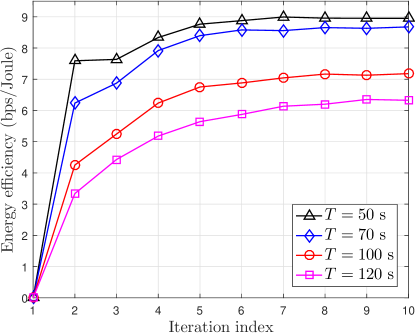
Figure 2: The EE versus the number of iterations for different flying periods.

The behavior of Algorithm 2 for various flying periods is shown in Fig. 2. The convergence is deemed to be attained when the increase of the EE is less than $\hat{\xi}=0.01$. As seen from Fig. 2, the EE rises quickly and then levels off as the number of iterations increases, eventually converging in 10 iterations.

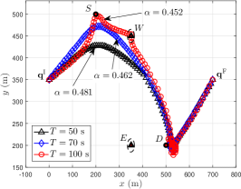
(a) The trajectory of $R$.

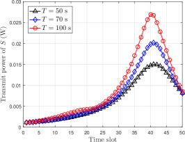
(b) The transmit power of $S$.

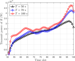
(c) The transmit power of $R$.

Figure 3: Optimized trajectory and transmit power with different flying period $T$.

The optimal trajectory and transmit power with different flying period $T$ are depicted in Fig. 3, where $T$ is equal to $50$ s, $70$ s, $100$ s, respectively. Fig. 3(a) clearly shows that in the first phase, as $T$ rises, $R$ gains greater maneuverability to approach the ground units ($S$ and $W$), leading to enhanced air-ground channels for both receiving and jamming, which in turn enables $S$ to transmit more power. And, in the second phase, it is typical for $R$ to maneuver away from $E$ in order to avoid wiretap. Alternately, it is an undisputed fact that an increase in $T$ leads to a decrease in the optimal time switching factor, $\alpha$. This is due to the introduction of collaborative interference, the first phase of the system achieves a higher achievable rate compared to the second phase. In order to maintain an excellent average achievable rate under the DF protocol, a smaller value of $\alpha$ is set with an increase in $T$. This assertion clearly indicates that $\alpha$ is a crucial factor that must be taken into consideration while making impactful decisions.

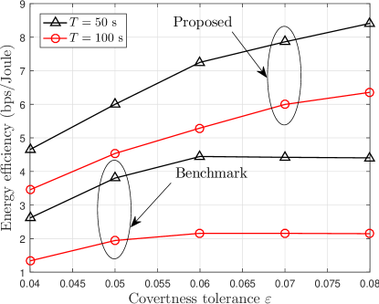
Figure 4: The impact of varying covertness tolerance $\varepsilon$.

To demonstrate the effect of varying covertness tolerance $\varepsilon$, the curve about the EE with a benchmark in which $R$ works with fixed trajectory is shown in Fig. 4. As the value of $\varepsilon$ increases, the graphs corresponding to both the proposed and benchmark display an upward trend. This is because when the tolerance level goes up, it becomes easier to meet the requirement for covertness which enables the transmitter $S$ to transmit higher power. Meanwhile, as $\varepsilon$ exceed a certain degree, the trend of increasing EE is starting to level off, particularly in the curve displayed in the benchmark scheme. This suggests that merely increasing covertness tolerance does not always result in substantial EE gains. Instead, it can expose confidential information to potential threats.

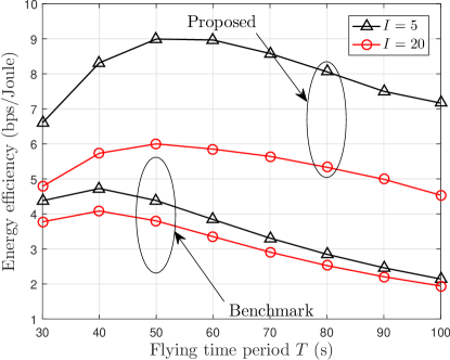
Figure 5: The EE versus varying flying period $T$.

For two different $W$’s observation times $I$, Fig. 5 illustrates the trend in EE with rising flying period $T$. Different from the relationship shown in Fig. 4 between EE and covertness tolerance, when it comes to increased flight period, EE follows a different pattern. Initially, it increases, then starts declining after reaching a certain degree, and eventually flattens out gradually. The underlying reason is that the initial gain in achievable rate resulting from an increase in flight time is far greater than the associated energy loss. However, beyond a certain threshold, the gain in achievable rate no longer compensates for the energy loss incurred, leading to a decline in EE. This phenomenon highlights the criticality of the selection of flight period $T$ in achieving optimal EE performance.

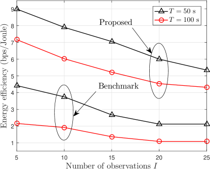
Figure 6: The effect of the number of observations $I$ conducted by $W$.

Fig. 6 examines how the number of observations conducted by $W$, $I$, affects the EE. One can see that when observation times rise, the EE has a decreasing trend. This is because, for $W$, additional observations allow for more detail to reduce the likelihood of detection errors and improve detection performance. Under the above circumstances, to achieve the same quality of communication covertness, $S$ needs to reduce the transmission power, thereby resulting in a decrease in EE. Ultimately, the proposed scheme outperforms the benchmark in terms of EE for all parameters considered in Figs. 4 - 6, demonstrating its superiority.

V Conclusion

In this work, a UAV relay assisted cooperative jamming covert and secrecy communication framework that considers the practical case of uncertain malicious nodes’ location was investigated. By designing the trajectory of the UAV, the transmit power of the transmitter and the time switching factor to maximize the EE, a robust FP optimization problem was established. To deal with this multivariate couple non-convex FP optimization problem, an efficient algorithm was proposed based on AO, primal-dual search and SCA methods to obtain a sub-optimal solution. Finally, numerical results exhibited the efficiency and superiority of the proposed algorithm and each parameter’s impact on the EE.

Appendix A Proof of Lemma 1

As an alternative, an upper bound on ${\cal D}\left({{\rm{P}}_{0}^{I}||{\rm{P}}_{1}^{I}}\right)$ is first focused, specifically

$$f\left({{\gamma_{W}}\left(n\right)}\right)=I\left({\ln\left({1+{\gamma_{W}}\left(n\right)}\right)-\frac{{{\gamma_{W}}\left(n\right)}}{{2\left({1+{\gamma_{W}}\left(n\right)}\right)}}}\right),$$ (34)

where ${\gamma_{W}}\left(n\right)>0$. Then, the $\frac{{df\left({{\gamma_{W}}\left(n\right)}\right)}}{{d{\gamma_{W}}\left(n\right)}}$ and $\frac{{{d^{2}}f\left({{\gamma_{W}}\left(n\right)}\right)}}{{d{\gamma_{W}}{{\left(n\right)}^{2}}}}$ are derived as $\frac{{I\left({1+2{\gamma_{W}}\left(n\right)}\right)}}{{2{{\left({1+{\gamma_{W}}\left(n\right)}\right)}^{2}}}}$ and $\frac{{-I{\gamma_{W}}\left(n\right)}}{{{{\left({1+{\gamma_{W}}\left(n\right)}\right)}^{3}}}}$, respectively. Since $\frac{{-I{\gamma_{W}}\left(n\right)}}{{{{\left({1+{\gamma_{W}}\left(n\right)}\right)}^{3}}}}<0$, $f\left({{\gamma_{W}}\left(n\right)}\right)$ is a concave function with respect to ${\gamma_{W}}\left(n\right)$. As a well-established concept, $\sqrt{x}$ is a monotonically increasing concave function with respect to $x$ [32]. Subsequently, according the convexity preserving property [32], $\sqrt{\frac{1}{2}f\left({{\gamma_{W}}\left(n\right)}\right)}$ is a concave function with respect to ${\gamma_{W}}\left(n\right)$. Then, via Jensen’s inequality [32], the following relationship is satisfied

$${{\mathbb{E}}_{\zeta}} \left({\sqrt{\frac{1}{2}f\left({{\gamma_{W}}\left(n\right)}\right)}}\right)$$ (35)

$$\leq\underbrace{\sqrt{\frac{I}{2}\left({\ln\left({1+{{\bar{\gamma}}_{W}}\left(n\right)}\right)-\frac{{{{\bar{\gamma}}_{W}}\left(n\right)}}{{2\left({1+{{\bar{\gamma}}_{W}}\left(n\right)}\right)}}}\right)}}_{\buildrel\Delta\over{=}g\left({{{\bar{\gamma}}_{W}}\left(n\right)}\right)},$$

where ${\bar{\gamma}_{W}}\left(n\right)=\frac{{{P_{S}}\left(n\right){{\left|{{{\bar{h}}_{SW}}}\right|}^{2}}}}{{P_{R}^{J}{{\left|{{h_{RW}}\left(n\right)}\right|}^{2}}+{\sigma^{2}}}}$ and ${\bar{h}_{SW}}=\sqrt{\frac{{{\beta_{0}}}}{{{{\left\|{{{\bf{q}}_{S}}-{{\bf{q}}_{W}}}\right\|}^{\eta}}}}}$. Thus, ${{\mathbb{E}}_{\zeta}}\left({\sqrt{\frac{1}{2}{\cal D}\left({{\rm{P}}_{0}^{I}||{\rm{P}}_{1}^{I}}\right)}}\right)<g\left({{{\bar{\gamma}}_{W}}\left(n\right)}\right)$ is established. For (17b), a new shrunken constraint $1-g\left({{{\bar{\gamma}}_{W}}\left(n\right)}\right)\geq 1-\varepsilon$ is built. Due to $g\left({{{\bar{\gamma}}_{W}}\left(n\right)}\right)$ is monotonically increasing with respect to ${{{\bar{\gamma}}_{W}}\left(n\right)}$, the new constraint can be equivalently transformed as follows via bisection search method, namely ${\bar{\gamma}_{W}}\left(n\right)\leq{\gamma_{\max}}$, where ${\gamma_{\max}}$ is equivalent threshold value, i.e., ${\gamma_{\max}}=g^{-1}\left(\varepsilon\right)$. Whereas, on account of the presence of estimation error in ${\bar{\gamma}_{W}}\left(n\right)$, the constraint ${\bar{\gamma}_{W}}\left(n\right)\leq{\gamma_{\max}}$ becomes indeterminate. As a solution, triangle inequality is applied to establish a certain upper bound. Conclusively, the more stringent covertness constraint is expressed as $\bar{\gamma}_{W}^{\sec}\left(n\right)\leq{\gamma_{\max}}$, where $\bar{\gamma}_{W}^{\sec}\left(n\right)=\frac{{{P_{S}}\left(n\right){{\left|{\bar{h}_{SW}^{\sec}}\right|}^{2}}}}{{P_{R}^{J}{{\left|{h_{RW}^{\sec}\left(n\right)}\right|}^{2}}+{\sigma^{2}}}}$, $\bar{h}_{SW}^{\sec}=\sqrt{\frac{{{\beta_{0}}}}{{{{\left|{\left\|{{{\bf{q}}_{S}}-{{{\bf{\hat{q}}}}_{W}}}\right\|-{r_{W}}}\right|}^{\eta}}}}}\geq{\bar{h}_{SW}}$ and $h_{RW}^{\sec}\left(n\right)=\sqrt{\frac{{{\beta_{0}}}}{{{{\left({\left\|{{{\bf{q}}_{R}}\left(n\right)-{{{\bf{\hat{q}}}}_{W}}}\right\|+{r_{W}}}\right)}^{2}}+{H^{2}}}}}\leq{h_{RW}}\left(n\right)$.

References

• [1] Y. Zeng, R. Zhang, and T. J. Lim, “Wireless communications with unmanned aerial vehicles: Opportunities and challenges,” IEEE Commun. Mag., vol. 54, no. 5, pp. 36-42, May 2016.
• [2] H. Kim, L. Mokdad, and J. Ben-Othman, “Designing UAV surveillance frameworks for smart city and extensive ocean with differential perspectives,” IEEE Commun. Mag., vol. 56, no. 4, pp. 98-104, Apr. 2018.
• [3] X. Lin, V. Yajnanarayana, S. D. Muruganathan, S. Gao, H. Asplund, H.-L. M¨a¨att¨anen, M. Bergstr¨om, S. Euler, and Y.-P. E. Wang, “The sky is not the limit: LTE for unmanned aerial vehicles,” IEEE Commun. Mag., vol. 56, no. 4, pp. 204-210, Apr. 2018.
• [4] N. Zhao, W. Lu, M. Sheng, Y. Chen, J. Tang, F. R. Yu, and K.-K. Wong, “UAV-assisted emergency networks in disasters,” IEEE Wireless Commun., vol. 26, no. 1, pp. 45-51, Feb. 2019.
• [5] Q. Wu, L. Liu, and R. Zhang, “Fundamental trade-offs in communication and trajectory design for UAV-enabled wireless network,” IEEE Wireless Commun., vol. 26, no. 1, pp. 36-44, Feb. 2019.
• [6] B. Duo, J. Luo, Y. Li, H. Hu, and Z. Wang, “Joint trajectory and power optimization for securing UAV communications against active eavesdropping,” China Commun., vol. 18, no. 1, pp. 88-99, Jan. 2021.
• [7] X. Chen, J. An, N. Zhao, C. Xing, D. B. da Costa, Y. Li, and F. R. Yu, “UAV relayed covert wireless networks: Expand hiding range via drones,” IEEE Netw., vol. 36, no. 4, pp. 226-232, Aug. 2022.
• [8] X. Chen, D. Li, Z. Yang, Y. Chen, N. Zhao, Z. Ding, and F. R. Yu, ”Securing aerial-ground transmission for NOMA-UAV networks,” IEEE Netw., vol. 34, no. 6, pp. 171-177, Dec. 2020.
• [9] X. Jiang, X. Chen, J. Tang, N. Zhao, X. Y. Zhang, D. Niyato, and K.-K. Wong, “Covert communication in UAV-assisted air-ground networks,” IEEE Wireless Commun., vol. 28, no. 4, pp. 190-197, Aug. 2021.
• [10] B. Yang, T. Taleb, G. Chen, and S. Shen, ”Covert communication for cellular and X2U-enabled UAV networks with active and passive wardens,” IEEE Netw., vol. 36, no. 1, pp. 166-173, Mar. 2022.
• [11] J. M. Hamamreh, H. M. Furqan, and H. Arslan, ”Classifications and applications of physical layer security techniques for confidentiality: A comprehensive survey,” IEEE Commun. Surveys Tuts., vol. 21, no. 2, pp. 1773-1828, May 2019.
• [12] Y. Cai, F. Cui, Q. Shi, M. Zhao, and G. Y. Li, “Dual-UAV-enabled secure communications: Joint trajectory design and user scheduling,” IEEE J. Sel. Areas Commun., vol. 36, no. 9, pp. 1972-1985, Sept. 2018.
• [13] W. Wang, X. Li, R. Wang, K. Cumanan, W. Feng, Z. Ding, and O. A. Dobre, “Robust 3D-trajectory and time switching optimization for dual-UAV-enabled secure communications,” IEEE J. Sel. Areas Commun., vol. 39, no. 11, pp. 3334-3347, Nov. 2021.
• [14] R. Zhang, X. Pang, W. Lu, N. Zhao, Y. Chen, and D. Niyato, “Dual-UAV enabled secure data collection with propulsion limitation,” IEEE Trans. Wireless Commun., vol. 20, no. 11, pp. 7445-7459, Jun. 2021.
• [15] M. Cui, G. Zhang, Q. Wu, and D. W. K. Ng, “Robust trajectory and transmit power design for secure UAV communications,” IEEE Trans. Veh. Technol., vol. 67, no. 9, pp. 9042-9046, Sept. 2018.
• [16] G. Zhang, Q. Wu, M. Cui, and R. Zhang, “Securing UAV communications via joint trajectory and power control,” IEEE Trans. Wireless Commun., vol. 18, no. 2, pp. 1376-1389, Feb. 2019.
• [17] B. Duo, Q. Wu, X. Yuan, and R. Zhang, “Energy efficiency maximization for full-duplex UAV secrecy communication,” IEEE Trans. Veh. Technol., vol. 69, no. 4, pp. 4590–4595, 2020.
• [18] B. A. Bash, D. Goeckel, D. Towsley, and S. Guha, “Hiding information in noise: Fundamental limits of covert wireless communication,” IEEE Commun. Mag., vol. 53, no. 12, pp. 26-31, Dec. 2015.
• [19] X. Chen, J. An, Z. Xiong, C. Xing, N. Zhao, F. R. Yu, and A. Nallanathan, “Covert communications: A comprehensive survey,” IEEE Commun. Surveys Tuts., vol. 25, no. 2, pp. 1173-1198, May 2023.
• [20] S. Yan, B. He, X. Zhou, Y. Cong, and A. L. Swindlehurst, ”Delay-intolerant covert communications with either fixed or random transmit power,” IEEE Trans. Inf. Forensics Security, vol. 14, no. 1, pp. 129-140, Jul. 2019.
• [21] X. Zhou, S. Yan, J. Hu, J. Sun, J. Li, and F. Shu, “Joint optimization of a UAV’s trajectory and transmit power for covert communications,” IEEE Trans. Signal Process., vol. 67, no. 16, pp. 4276-4290, Aug. 2019.
• [22] M. Li, X. Tao, H. Wu, and N. Li, ”Joint trajectory and resource optimization for covert communication in UAV-enabled relaying systems,” IEEE Trans. Veh. Technol., vol. 72, no. 4, pp. 5518-5523, Apr. 2023.
• [23] X. Chen, N. Zhang, J. Tang, M. Liu, N. Zhao, and D. Niyato, “UAV-aided covert communication with a multi-antenna jammer,” IEEE Trans. Veh. Technol., vol. 70, no. 11, pp. 11 619-11 631, Nov. 2021.
• [24] H. Lei, J. Jiang, I. S. Ansari, G. Pan, and M.-S. Alouini, ”Trajectory and power design for aerial multi-user covert communications,” IEEE Trans. Aerosp. Electron. Syst., doi: 10.1109/taes.2024.3378203, pp. 1-15, Mar. 2024.
• [25] C. Wang, X. Chen, J. An, Z. Xiong, C. Xing, N. Zhao, and D. Niyato, “Covert communication assisted by UAV-IRS,” IEEE Trans. Commun., vol. 71, no. 1, pp. 357-369, Jan. 2023.
• [26] F. Yang, C. Wang, J. Xiong, N. Deng, N. Zhao, and Y. Li, ”UAV-enabled robust covert communication against active wardens,” IEEE Trans. Veh. Technol., doi: 10.1109/tvt.2024.3360998, pp. 1-6, Jan. 2024.
• [27] C. Wang, Z. Li, H. B. Zhang, D. W. K. Ng, and N. Al-Dhahir, “Achieving covertness and security in broadcast channels with finite blocklength,” IEEE Trans. Wireless Commun., vol. 21, no. 9, pp. 7624-7640, Sept. 2022.
• [28] P. Liu, Z. Li, J. Si, N. Al-Dhahir, and Y. Gao, ”Joint information-theoretic secrecy and covertness for UAV-assisted wireless transmission with finite blocklength,” IEEE Trans. Veh. Technol., vol. 72, no. 8, pp. 10187-10199, Aug. 2023.
• [29] Y. Zeng, J. Xu, and R. Zhang, “Energy minimization for wireless communication with rotary-wing UAV,” IEEE Trans. Wireless Commun., vol. 18, no. 4, pp. 2329-2345, Apr. 2019.
• [30] E. L. Lehmann and J. P. Romano, Testing Statistical Hypotheses. Berlin, Germany: Springer, 2006.
• [31] J. P. Crouzeix, J. A. Ferland, S. Schaible, “An algorithm for generalized fractional programs,” Journal of Optimization Theory and Applications, vol.47, no.1, pp.35-49, Sep. 1985.
• [32] S. Boyd and L. Vandenberghe, Convex Optimization. Cambridge, U.K.: Cambridge Univ. Press, 2004.