Cosmological Stasis from Dynamical Scalars:
Tracking Solutions and the Possibility of a Stasis-Induced Inflation

Abstract

It has recently been realized that many theories of physics beyond the Standard Model give rise to cosmological histories exhibiting extended epochs of cosmological stasis. During such epochs, the abundances of different energy components such as matter, radiation, and vacuum energy each remain fixed despite cosmological expansion. In previous analyses of the stasis phenomenon, these different energy components were modeled as fluids with fixed, unchanging equations of state. In this paper, by contrast, we consider more realistic systems involving dynamical scalars which pass through underdamping transitions as the universe expands. Indeed, such systems might be highly relevant for BSM scenarios involving higher-dimensional bulk moduli and inflatons. Remarkably, we find that stasis emerges even in such situations, despite the appearance of time-varying equations of state. Moreover, this stasis includes several new features which might have important phenomenological implications and applications. For example, in the presence of an additional “background” energy component, we find that the scalars evolve into a “tracking” stasis in which the stasis equation of state automatically tracks that of the background. This phenomenon exists even if the background has only a small initial abundance. We also discuss the intriguing possibility that our results might form the basis of a new “Stasis Inflation” scenario in which no ad-hoc inflaton potential is needed and in which there is no graceful-exit problem. Within such a scenario, the number of $e$-folds of cosmological expansion produced is directly related to the hierarchies between physical BSM mass scales. Moreover, non-zero matter and radiation abundances can be sustained throughout the inflationary epoch.

I Introduction, motivation, and overview of results

Cosmological stasis Dienes et al. (2022a, 2024) is a surprising phenomenon wherein the abundances of multiple cosmological energy components (e.g., matter, radiation, vacuum energy, etc.)  with different equations of state each remain constant over an extended period, despite the effects of Hubble expansion. This phenomenon has been shown to arise in new-physics scenarios involving towers of unstable particles Dienes et al. (2022a), theories involving populations of scalars undergoing underdamping transitions Dienes et al. (2024), and even theories with populations of primordial black holes with extended mass spectra Barrow et al. (1991); Dienes et al. (2022b).

In all of these realizations of stasis, the energy densities of the different energy components involved scale differently under cosmological expansion because they have different equations of state. Thus, a priori, one might expect their respective abundances to change rapidly as the universe expands. However, these changes in the abundances of the different energy components can be compensated by processes that actually transfer energy between these different components. In this way, each of the different abundances can potentially remain constant.

At first glance, it might seem that one must carefully balance the effects of these energy-transferring processes against the effects of cosmological expansion in order to achieve stasis. If true, this would render stasis the result of a severe fine-tuning. However, as shown in Refs. Dienes et al. (2022a, b, 2024); Barrow et al. (1991), the required balancing is actually a global attractor within the coupled system of Boltzmann and Einstein equations that govern the cosmological evolution of the abundances. The universe will thus necessarily evolve towards (and eventually enter) stasis irrespective of initial conditions.

There exist many different examples of such energy-transferring processes. These in turn depend on the particular model of stasis under study. For example, in models exhibiting a stasis between particulate matter and radiation, as discussed in Refs. Dienes et al. (2022a, 2024), the relevant energy-transferring process was particle decay. Likewise, in models of matter/radiation stasis in which the matter takes the form of primordial black holes Barrow et al. (1991); Dienes et al. (2022b), the relevant energy-transferring process was Hawking evaporation. Indeed, both particle decay and Hawking radiation convert matter energy to radiation energy and therefore play an integral role in keeping the abundances of matter and radiation constant despite cosmological expansion.

In Ref. Dienes et al. (2024), by contrast, it was shown that stasis can also arise between vacuum energy and matter. In fact, it was even shown that one can have a triple stasis between vacuum energy, matter, and radiation simultaneously Dienes et al. (2024). The underlying model that was analyzed for these purposes was built upon the dynamical evolutions of the homogeneous zero-mode field values associated with a tower of scalar fields. As is well known, each such field value evolves according to an equation of motion which resembles that of a massive harmonic oscillator with a Hubble-induced “friction” term. Within an expanding universe, the Hubble-friction term is large at early times, and thus our field is overdamped. In this case, the potential energy of the field vastly exceeds its kinetic energy, whereupon the energy density of this field may be viewed as pure potential energy (i.e., vacuum energy), with an equation-of-state parameter $w\approx-1$. However, as the universe continues to expand, the Hubble parameter drops, eventually reaching (and passing through) a critical point at which our system becomes underdamped and our field begins to oscillate and eventually virialize. During such an oscillatory phase, the kinetic and potential energies associated with our field are then approximately equal, whereupon we find that $w\approx 0$. This transition from an overdamped phase to an underdamped phase may thus be regarded as an energy-transferring process in which the corresponding energy density transitions from vacuum energy to matter.

In each of these previous realizations of the stasis phenomenon, the corresponding energy densities were modeled as fluids with time-independent equations of state. Indeed, in cases involving stases between matter and radiation — such as were discussed in Refs. Dienes et al. (2022a, 2024) — the matter and radiation were modeled as fluids with constant equation-of-state parameters $w=0$ and $w=1/3$, respectively. Given that the physics in these cases rested on either particle decay or Hawking radiation, this can be viewed as a natural and reasonable assumption.

For calculational simplicity, the same assumption was also made in Ref. Dienes et al. (2024) when considering the dynamical evolution of the homogeneous zero-mode field value associated with a scalar field. In particular, the energy density associated with such a field was treated in Ref. Dienes et al. (2024) as that of a fluid with a constant equation-of-state parameter $w=0$ throughout the later, underdamped phase, and treated as that of a fluid with a constant equation-of-state parameter $w$ near $-1$ throughout the earlier, overdamped phase. Moreover, the transition between these two phases of the theory was treated as instantaneous, occurring at the critical time at which the underdamping transition normally takes place in the fully dynamical theory. Given these assumptions, it was then found that a stasis also emerged between these two fluids — a stasis which was interpreted as existing between vacuum energy and matter. Moreover, as noted above, allowing these fields to decay after transitioning from vacuum energy to matter was then shown to result in a triple stasis between vacuum energy, matter, and radiation.

While such results are exciting and may have many phenomenological implications, the true dynamical evolution of a scalar field in a cosmological setting is more complicated than this. As noted above, the true dynamics of such a field is governed by an equation of motion which is that of a damped harmonic oscillator. Within such a system, there continues to exist a critical boundary between an overdamped and underdamped phase as the Hubble-friction term decreases over time. However, the equation-of-state parameter prior to this transition is not fixed at a small value near $w\approx-1$ within the overdamped phase, nor is it (or its virial time-average) fixed at $w=0$ within the subsequent underdamped phase. Instead, the true behavior of our dynamical scalar field is an entirely smooth one. The corresponding equation-of-state parameter will indeed asymptote to a fixed value near $w=-1$ at increasingly early times — an epoch during which the corresponding field $\phi_{\ell}$ remains fixed or at most slowly rolls — and likewise it will asymptote to the fixed time-averaged value $w=0$ at increasingly late times, an epoch during which the field experiences rapid virialized oscillations. However, between these asymptotic limits, our scalar field and its equation of state are both evolving dynamically in a smooth, non-trivial, time-dependent manner. This evolution does not even exhibit a sharp change of behavior of any sort as our system passes through the critical underdamping transition.

In this paper, we seek to determine what happens to our stasis phenomenon when we take this full time-dependence into account. At first glance, it might seem that including this time dependence for the equation-of-state parameters for the individual scalar fields would completely destabilize the stasis that emerges when these equation-of-state parameters are instead taken to be constant both before and after the underdamping transition. Indeed, such time-dependent equation of state parameters could in principle complicate the manner in which the Hubble parameter evolves with time, and thus lead to a more complicated dynamical evolution for our scalar fields and their corresponding energy densities. However, since stasis is built on the idea that the abundances of our different fluids remain constant despite cosmological expansion, it is a natural expectation that allowing for time-varying equation-of-state parameters would destroy the stasis that is observed when these equation-of-state parameters are constant.

Remarkably, in this paper we find that stasis can emerge even in such situations. In particular, we find that there exists a large class of scenarios in which stasis emerges as an attractor — the time-variation of the equation-of-state parameters for the individual fields notwithstanding — and persists across many $e$-folds of cosmological expansion. In this regard, then, our results are similar to those of Refs. Dienes et al. (2022a, 2024) and demonstrate that the stasis phenomenon exists even for dynamical scalars when their full time dependence is taken into account.

Despite this similarity, we shall find that the stasis that is realized through fully dynamical scalars has a number of additional properties that transcend those arising within the previous realizations of stasis which have been identified. In particular, we shall find that the fundamental constraint equation that underlies this stasis does not uniquely predict the equation of state of our system once it has entered stasis. This gives our dynamical-scalar stasis a certain intrinsic mathematical flexibility that was not previously available.

As we shall find, the full implications of this additional flexibility are particularly significant when this stasis is realized in the presence of an additional “background spectator” fluid — i.e., a fluid which is completely inert, neither receiving energy from our stasis system nor donating energy to it. Indeed, regardless of the initial abundance and equation-of-state parameter which are assumed for this background fluid, we find not only that our stasis solution continues to exist, but that it actually has the flexibility needed in order to track this fluid, automatically adjusting its properties such that the resulting equation-of-state parameter $w_{\rm univ}$ for the universe as a whole during stasis matches that of the background. This is thus our first example of a “tracking” stasis. Indeed, we find that this tracking property persists even if the equation of state for the background fluid changes with time.

This realization of stasis involving dynamical scalars also has another important property: as we shall see, it can easily accommodate an equation-of-state parameter for the universe within the range $-1<w_{\rm univ}<-1/3$. A stasis epoch in which $w_{\rm univ}$ falls within this range constitutes a period of accelerated cosmological expansion in which $\ddot{a}>0$, where $a$ is the scale factor. Since a stasis epoch of this sort can span many $e$-folds of expansion, such a epoch can serve as a means of addressing the horizon and flatness problems. This observation suggests that stasis could potentially serve as a novel mechanism for achieving cosmic inflation. No non-trivial, ad-hoc inflaton potential would be required within such a “Stasis Inflation” scenario; likewise, this scenario has no graceful-exit problem. Moreover, non-zero matter and radiation abundances can be sustained throughout an inflationary epoch of this sort. In this paper, we shall discuss this new “Stasis Inflation” possibility and outline some of its key qualitative features. Of course, further analysis will be required in order to determine whether such an inflation scenario is truly viable.

This paper is organized as follows. In Sect. II, we review the dynamical evolution of a single scalar field which undergoes a transition from overdamped rolling to underdamped oscillation. In Sect. III, we then extend this single-field analysis to the more general case in which the particle content of the theory includes a tower of scalar fields $\phi_{\ell}$ with a non-trivial spectrum of masses and initial abundances. Despite the non-trivial manner in which the individual equation-of-state parameters $w_{\ell}(t)$ for these scalars each evolve in time, we nevertheless find that the tower as a whole can give rise to a stasis epoch in which the effective equation-of-state parameter for the universe as a whole is essentially constant. In Sect. IV, we then consider how the resulting cosmological dynamics is modified in the presence of an additional background energy component with an equation-of-state parameter $w_{\rm BG}$. We find that the tower of scalars can still reach a stasis. In fact, for certain values of $w_{\rm BG}$, we find that the equation-of-state parameter for the tower evolves toward $w_{\rm BG}$ and tracks it, even in situations in which $w_{\rm BG}$ exhibits a non-trivial time-dependence. In Sect. V, we then discuss the possibility of a stasis-induced inflationary epoch during which our stasis itself drives an accelerated expansion of the universe. Finally, in Sect. VI, we conclude with a summary of our main results and a discussion of possible avenues for future work.

II A single scalar in an expanding universe

Let us start by reviewing the dynamical evolution of a single real scalar field $\phi$ in an expanding universe. In general, the energy density and pressure of such a scalar field are given by

$$\rho_{\phi}~{}=~{}\frac{1}{2}\dot{\phi}^{2}+V\,,~{}~{}~{}P_{\phi}~{}=~{}\frac{1}{2}\dot{\phi}^{2}-V\,,$$ (1)

where the “dot” denotes the derivative with respect to the time $t$ in the cosmological background frame and where $V(\phi)$ is the scalar potential. The equation-of-state parameter for this field is therefore thus given by

$$w_{\phi}~{}\equiv~{}\frac{P_{\phi}}{\rho_{\phi}}~{}=~{}\frac{\frac{1}{2}\dot{\phi}^{2}-V}{\frac{1}{2}\dot{\phi}^{2}+V}~{}.$$ (2)

In general, $w_{\phi}$ is time-dependent and can vary continuously within the range $-1\leq w_{\phi}\leq 1$.

The dynamics of this scalar field is governed by its equation of motion

$$\ddot{\phi}+3H\dot{\phi}+\frac{dV}{d\phi}~{}=~{}0\,,$$ (3)

where the effects of the FRW cosmology (i.e., the effects coming from the expansion of the universe) are encoded within the time-dependence of the Hubble parameter $H\equiv\dot{a}/a$. As evident from Eq. (3), the Hubble parameter affects the evolution of the scalar by providing a source of “friction” which damps the motion of the scalar. The value of $H$ is related to the total energy density $\rho_{\rm tot}$ of the universe through the Friedmann equation

$$H^{2}~{}=~{}\frac{8\pi G}{3}\rho_{\rm tot}~{}=~{}\frac{\rho_{\rm tot}}{3M_{P}^{2}}\,,$$ (4)

where $M_{P}=1/\sqrt{8\pi G}$ is the reduced Planck mass. A larger value of $\rho_{\rm tot}$ therefore corresponds to a larger damping term for $\phi$ and vice versa. Moreover, in this paper we shall also make the “minimal” assumption that the potential is quadratic — i.e., that

$$V(\phi)~{}=~{}\frac{1}{2}m^{2}\phi^{2}~{},$$ (5)

where $m$ is the mass of $\phi$.

In general, the solutions to Eq. (3) will depend critically on the size of the Hubble-friction term. When this term is sufficiently small, the system is underdamped and the value of $\phi$ oscillates with a decreasing amplitude. By contrast, if the Hubble-friction term is sufficiently large, the system is overdamped and $\phi$ either remains effectively constant or decreases slowly without oscillating. However, within a given cosmology, $H(t)$ generally decreases as a function of $t$. Thus, even if $\phi$ is initially in the overdamped phase, it will eventually transition to the underdamped phase when $H(t)$ drops below the critical value $H(t)=2m/3$.

As a result of these features, it is of great interest to understand how $\rho_{\rm tot}$ (and therefore $H$) varies with time. In particular, we shall focus on two cases of interest which represent different possible relationships between $\rho_{\phi}$ and $\rho_{\rm tot}$:

• Case I: In addition to $\phi$, the universe contains another cosmological energy component with a constant equation-of-state parameter $w$. This additional energy component is assumed to dominate the energy density of the universe during the time period of interest. Since $\rho_{\phi}\ll\rho_{\rm tot}$, the evolution of $H$ is essentially independent of $\rho_{\phi}$ throughout this time period.

• Case II: The field $\phi$ is the only cosmological energy component with non-negligible energy density. Thus, to a good approximation, we may take $\rho_{\rm tot}=\rho_{\phi}$.

Both of these cases have been studied extensively, and we shall review the cosmological dynamics which emerges in each case in turn.

II.1 Case I:  Fixed external cosmology

During any epoch wherein the universe is dominated by a cosmological energy component with a fixed equation-of-state parameter $w$, the Hubble parameter is given by $H=\kappa/(3t)$ with $\kappa=2/(1+w)$. It therefore follows that in Case I, Eq. (3) reduces to

$$\phi^{\prime\prime}+\frac{\kappa}{\tilde{t}}\phi^{\prime}+\phi~{}=~{}0\,,$$ (6)

where $\tilde{t}\equiv mt$ is a dimensionless time variable and where a prime denotes a derivative with respect to $\tilde{t}$. The general solution to this differential equation takes the form

$$\phi(\tilde{t})~{}=~{}\tilde{t}^{(1-\kappa)/2}\left[c_{J}J_{(\kappa-1)/2}(\tilde{t})+c_{Y}Y_{(\kappa-1)/2}(\tilde{t})\right]\,,$$ (7)

where $J_{\nu}(z)$ and $Y_{\nu}(z)$ are Bessel functions of the first and second kind, respectively, and where $c_{J}$ and $c_{Y}$ are coefficients with dimensions of mass. This solution for $\phi(\tilde{t})$ is plotted as a function of $\tilde{t}$ in Fig. 1.

It is also possible to obtain an approximate solution for $\tilde{t}\ll 1$. For $z\ll 1$, the Bessel functions $J_{\nu}(z)$ and $Y_{\nu}(z)$ are well approximated by $J_{\nu}(z)\sim z^{\nu}$ and $Y_{\nu}(z)\sim-z^{-\nu}$. Thus, if the initial conditions for $\phi$ at some early dimensionless time $\tilde{t}^{(0)}\ll 1$ are such that $\phi^{(0)}\equiv\phi(\tilde{t}^{(0)})\not=0$ and $\phi^{\prime}(\tilde{t}^{(0)})\approx 0$, one may take $c_{Y}\approx 0$ and thereby obtain the approximate solution

$$\phi(\tilde{t})~{}\approx~{}c_{J}\,\tilde{t}^{(1-\kappa)/2}J_{(\kappa-1)/2}(\tilde{t})\,.$$ (8)

This expression provides an excellent approximation to the full numerical solution for $\phi(\tilde{t})$ shown in Fig. 1. Indeed, a plot of this approximate expression would be indistinguishable to the naked eye from the full solution over the entire range of $\tilde{t}$ shown.

As can be seen from Fig. 1, the expression for $\phi(\tilde{t})$ in Eq. (7) behaves like a damped oscillator. At early times, when $\tilde{t}\ll 1$, the field is overdamped due to the sizable Hubble-friction term. As a result, we find that $w_{\phi}\approx-1$ within this regime, and $\phi$ behaves like a vacuum-energy component. By contrast, at late times, when $\tilde{t}\gg 1$, both $\phi$ itself and $w_{\phi}$ oscillate rapidly. The amplitude of $\phi$ decreases with $\tilde{t}$ within this regime, and as a result we find $\rho_{\phi}\sim a^{-3}$, just as we would expect for the energy density of massive matter. Accordingly, while the amplitude of $w_{\phi}$ is effectively unity within this regime, the time-averaged value $\langle w_{\phi}\rangle_{t}$ of $w_{\phi}$ over a sufficiently long interval $\Delta\tilde{t}\equiv\tilde{t}-\tilde{t}^{(0)}$ approaches $\langle w_{\phi}\rangle_{t}\approx 0$.

The transition region between these two limiting regimes physically corresponds to the time window wherein $\phi$ is rolling down its potential $V(\phi)$ with non-negligible field velocity $\phi^{\prime}$, but has not yet reached the potential minimum at $\phi=0$. During this window, both $\phi$ and $w_{\phi}$ evolve non-trivially with $\tilde{t}$. Since this transition from overdamped and underdamped evolution occurs when $3H(t)\sim 2m$, as discussed above, it is conventional to define the critical time $t_{c}$ associated with this phase transition such that $\tilde{t}_{c}=\kappa/2$ in this case. However, this phase transition clearly is not instantaneous, and as we shall see, the manner in which scalar fields evolve during such transition windows has important implications for the cosmological dynamics which emerges when a tower of such scalars is present.

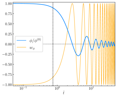
Figure 1: The value of the scalar field $\phi(\tilde{t})$, normalized to its asymptotic early-time value $\phi^{(0)}$ and plotted as a function of the dimensionless time variable $\tilde{t}$ during an epoch in which the energy density of the universe is dominated by a radiation component ($w=1/3$). Also shown is the corresponding equation-of-state parameter $w_{\phi}(\tilde{t})$. The curves shown here correspond to a choice of initial conditions in which $\phi^{(0)}\neq 0$ and $\phi^{\prime}(\tilde{t}^{(0)})=0$. The vertical dashed line at $\tilde{t}=\kappa/2$ indicates the critical value $\tilde{t}_{c}$ of $\tilde{t}$ associated with the transition from overdamped to underdamped evolution.

II.2 Case II:  Scalar domination

The cosmological dynamics which governs the evolution of $\phi$ and $H$ is significantly more complicated in Case II than in Case I due to the fact that $H$ now depends on $\phi$ itself. Indeed, in this case we find that Eq. (3) takes the form

$$\phi^{\prime\prime}+\frac{3H}{m}\phi^{\prime}+\phi~{}=~{}0\,$$ (9)

where from Eq. (4) we now have

$$H~{}=~{}\frac{m}{\sqrt{6}}\sqrt{\left(\frac{\phi}{M_{P}}\right)^{2}+\left(\frac{\phi^{\prime}}{M_{P}}\right)^{2}}\,.$$ (10)

This dependence of the Hubble parameter on $\phi$ and $\phi^{\prime}$ not only changes the time-evolution of $\phi$, but also introduces an added sensitivity of our system to its initial conditions. For example, changing the initial value of $\phi$ has the effect of changing the initial value of the Hubble parameter $H$, and as we shall see, this can in turn affect the length of time that must elapse before our system can reach critical milestones such as the transition to an underdamped phase.

Solutions to the non-linear differential equation in Eq. (9) may be obtained numerically. In examining the behavior of these solutions, we once again focus for simplicity on the case in which the initial conditions for $\phi$ at $\tilde{t}^{(0)}\ll 1$ are such that $\phi^{(0)}$ is non-vanishing, while $\phi^{\prime}(\tilde{t}^{(0)})\approx 0$. In Fig. 2, we show how $\phi(\tilde{t})$ evolves as a function of $\tilde{t}$ for several different values of $3H^{(0)}/2m$ — or, equivalently, since $3H^{(0)}/2m=\sqrt{3/8}\,|\phi^{(0)}|/M_{P}$ for this choice of initial conditions, for several different values of $\phi^{(0)}$. In the left panel, we normalize each $\phi(\tilde{t})$ curve to the corresponding initial field value $\phi^{(0)}$ and adopt a logarithmic scale for the horizontal axis. In the right panel, we show the same curves, but normalize each one to the fixed reference scale $M_{P}$ and adopt a linear scale for the horizontal axis.

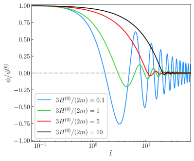
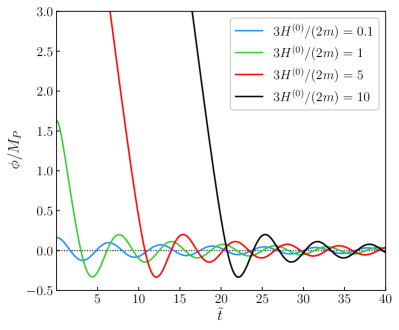
Figure 2: Left panel: The values of the scalar field $\phi(\tilde{t})$, normalized to their asymptotic early-time values $\phi^{(0)}$ and plotted as functions of the dimensionless time variable $\tilde{t}$ for a variety of different choices of $\phi^{(0)}$ during an epoch in which the energy density of the universe is dominated by $\phi$ itself. Note that varying $\phi^{(0)}$ for the same value of $m$ is tantamount to choosing different values of $3H^{(0)}/(2m)$. In all cases, we have taken $\phi^{\prime}(t^{(0)})=0$. Right panel: Same as in the left panel, but with $\phi$ normalized to the value of $M_{P}$ and with a linear rather than a logarithmic scale for the horizontal axis. Note that unlike the other curves, the blue curve always already begins in the underdamped regime.

For $3H^{(0)}/2m\gg 1$, the Hubble-friction term in Eq. (9) is sufficiently large that $\phi$ is initially overdamped as it begins rolling from rest toward its potential minimum. Within this “slow-roll” regime, $\phi^{\prime\prime}(\tilde{t})$ is negligible in comparison to the other two terms in Eq. (9), and therefore, to a good approximation, we have

$$\phi^{\prime}~{}\approx~{}-\frac{m}{3H}\phi\,.$$ (11)

The solutions for $\phi$ and $H$ within the slow-roll regime are therefore well approximated by

$$\phi(\tilde{t}) \approx \phi^{(0)}\exp\left[-\frac{1}{2}\int_{\tilde{t}^{(0)}}^{\tilde{t}}\frac{2m}{3H(\hat{t})}\,d\hat{t}\,\right]$$

$$H(\tilde{t}) \approx H^{(0)}\exp\left[-\frac{1}{2}\int_{\tilde{t}^{(0)}}^{\tilde{t}}\frac{2m}{3H(\hat{t}\,)}\,d\hat{t}\,\right]\,.$$ (12)

Since $\phi$ evolves extremely slowly within this regime, $3H/(2m)\gg 1$ remains large and $H(\tilde{t})\approx H^{(0)}$ is effectively constant. As a result, the universe experiences an epoch of accelerated expansion at early times. This epoch effectively ends at the time $t_{c}$ at which $3H(t_{c})=2m$ and the coefficient of the Hubble-friction term in Eq. (9) drops below the value associated with critical damping. At subsequent times $t>t_{c}$, the field experiences underdamped oscillations. The value of $\phi$ at $t_{c}$ is approximately independent of $\phi^{(0)}$ and given by

$$\phi(t_{c})~{}\approx~{}\frac{H(t_{c})}{H^{(0)}}\,\phi^{(0)}~{}=~{}\sqrt{\frac{8}{3}}M_{P}\,,$$ (13)

as is evident from the right panel of Fig. 2. However, as is evident from the left panel, this implies that the extent to which the field is suppressed at $t_{c}$ relative to its initial value at $t^{(0)}$ becomes more severe as $\phi^{(0)}$ increases. By contrast, in situations in which $3H^{(0)}/(2m)\ll 1$, such as that illustrated by the blue curve in each panel of the figure, the field is already underdamped at $t=t^{(0)}$, and oscillation commences immediately thereafter.

The difference between the initial time $t^{(0)}$ and the critical time $t_{c}$ can be quantified in terms of the parameter $\Delta\tilde{t}_{c}\equiv\tilde{t}_{c}-\tilde{t}^{(0)}$, which can be estimated by evaluating Eq. (12) at $\tilde{t}=\tilde{t}_{c}$. Doing this, we obtain

$$\Delta\tilde{t}_{c}~{}\approx~{}\left\langle\frac{m}{3H}\right\rangle_{t_{c}}^{-1}\log\left(\frac{3H^{(0)}}{2m}\right)\,,$$ (14)

where $\left\langle x\right\rangle_{t_{c}}$ denotes the time-average of the quantity $x$ over the time interval $\Delta t_{c}$. Since $H$ decreases less rapidly than $t^{-1}$ as a function of time while $\phi$ is slowly rolling, this time-average decreases with $H^{(0)}$. It therefore follows from the form of Eq. (14) that $\Delta\tilde{t}_{c}$ occurs later for larger $H^{(0)}$. The particular manner in which this delayed onset of oscillation manifests itself is illustrated in the right panel of Fig. 2. Indeed, by comparing the green, red and black curves shown in this panel, we observe that to a good approximation the functional forms of $\phi(\tilde{t})$ obtained for different $\phi^{(0)}$ differ only by a horizontal shift.

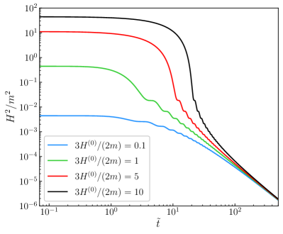
Figure 3: The ratio $H^{2}/m^{2}$, which is proportional to the total energy density $\rho_{\rm tot}$ of the universe, during an epoch wherein the energy density of the universe is dominated by $\phi$ itself. The different curves correspond to the same parameter choices adopted in Fig. 2. We observe that all of these curves — despite the different choices of initial conditions they each represent — asymptotically converge at late times to a power law which corresponds to a scaling behavior $\rho_{\rm tot}\sim a^{-3}$ at late times.

Eventually, at dimensionless times $\tilde{t}\gg\tilde{t}_{c}$, when $\phi(\tilde{t})$ is deep within the oscillatory phase, the time-average of the equation-of-state parameter over a sufficiently long time window becomes $\left\langle w_{\phi}\right\rangle_{t}\approx 0$, much as it does in Case I. Thus, as in Case I, we find $H\approx\kappa/(3t)$ with $\kappa=2$ for $\tilde{t}\gg\tilde{t}_{c}$. However, since $H^{2}\propto\rho_{\phi}$ in Case II, one finds that the total energy density of the universe approaches a universal functional form $\rho_{\rm\phi}\propto a^{-3}$ at late times, regardless of the choice of initial conditions. This behavior is illustrated in Fig. 3, which shows the evolution of the dimensionless ratio $H^{2}/m^{2}$ for a variety of different choices of $3H^{(0)}/(2m)$. Indeed, we observe that all the curves shown in Fig. 3 exhibit the same asymptotic functional form at large $\tilde{t}$.

Looking forward, one of our primary concerns in this paper is to understand the manner in which the zero-modes of dynamically evolving scalar fields might contribute to the development of a stasis epoch within the cosmological timeline. It is clear from the above analysis that a single such scalar field — whose zero-mode energy density transitions from slow-roll behavior to rapid oscillation over a relatively narrow time window — cannot give rise to a stasis epoch alone. However, as we shall see, many aspects of the dynamics of individual scalars that we have highlighted in this section will play an important role in establishing and sustaining stasis when multiple such fields are considered.

III Stasis from a tower of scalars

We shall now generalize the above analysis by replacing our single scalar field with an entire tower of scalar fields with different masses. Our goal will be to determine whether an epoch of stasis might arise from such a tower and what its properties might be.

III.1 Preliminaries

Let us now assume that there exists a tower of $N$ scalar fields $\phi_{\ell}$ in the early universe, each of which experiences a quadratic potential

$$V_{\ell}~{}=~{}\frac{1}{2}m_{\ell}^{2}\phi_{\ell}^{2}\,,$$ (15)

where the index $\ell=0,1,2,\dots,N-1$ labels the states in order of increasing mass. The equation of motion for each state is then

$$\ddot{\phi}_{\ell}+3H\dot{\phi}_{\ell}+m_{\ell}^{2}\phi_{\ell}~{}=~{}0~{},$$ (16)

while the energy density, pressure, equation-of-state parameter, and cosmological abundance of each state are given by

$$\rho_{\ell}~{} = ~{}\frac{1}{2}\dot{\phi}_{\ell}^{2}+\frac{1}{2}m_{\ell}^{2}\phi_{\ell}^{2}$$

$$P_{\ell}~{} = ~{}\frac{1}{2}\dot{\phi}_{\ell}^{2}-\frac{1}{2}m_{\ell}^{2}\phi_{\ell}^{2}$$

$$w_{\ell}~{} \equiv ~{}P_{\ell}/\rho_{\ell}$$

$$\Omega_{\ell}~{} \equiv ~{}\frac{\rho_{\ell}}{3H^{2}M_{P}^{2}}~{}.$$ (17)

Each of these quantities is generally time-dependent. We can also define the total abundance associated with our tower of states

$$\Omega_{\rm tow}(t)~{}\equiv~{}\sum_{\ell}\Omega_{\ell}(t)~{},$$ (18)

as well as the time-dependent effective equation-of-state parameter for our tower

$$\left\langle w\right\rangle(t)~{}\equiv~{}\frac{1}{\Omega_{\rm tow}(t)}\,\sum_{\ell}\Omega_{\ell}(t)\,w_{\ell}(t)~{}.$$ (19)

In general, we have $0\leq\Omega_{\rm tow}\leq 1$, with the value of $\Omega_{\rm tow}$ ultimately depending on what other energy components might also exist in the universe. Of course, if the total energy density of the universe is only that associated with the tower of $\phi_{\ell}$ states, we then have $\Omega_{\rm tow}=1$ at all times. However, until stated otherwise, we shall not make this assumption.

Along these lines, we note that $\Omega_{\rm tow}$ is not the only quantity whose value depends on the full energy content of the universe. Indeed, even the individual abundances $\Omega_{\ell}$ implicitly depend on the full energy content through their dependence on $H$, or simply because abundances generally indicate the fraction of energy density relative to the total energy density in the universe. Thus, for example, we see that the definition of $\langle w\rangle$ in Eq. (19) makes sense because it is invariant under such rescalings of the abundances.

At any specific time $t$, certain states within the tower may still be overdamped while others may have already become underdamped. We will respectively identify these groups of states as

• slow-roll components, which consist of the overdamped states with $m_{\ell}<3H(t)/2$; and

• oscillatory components, which are comprised of the underdamped states with $m_{\ell}\geq 3H(t)/2$.

Note that we shall use the terminology “slow-roll” (SR) and “oscillatory” (osc) to indicate whether a given state is overdamped or underdamped regardless of whether its field VEV is actually rolling or oscillating. Indeed, as we have seen in Sect. II, a given state near the transition time may be underdamped and not yet have begun to oscillate; likewise, a given state may be so severely overdamped that it is effectively stationary without any significant rolling behavior.

Let us define $\ell_{c}(t)$ to be the critical value of $\ell$ within the tower for which $3H(t)=2m_{\ell}$. More specifically, we shall implicitly assume that our spectrum of states is sufficiently dense that we may regard (or approximate) $\ell_{c}(t)$ as an integer at any time; this assumption will render our equations simpler but will not affect our final results. We shall also consider the “boundary” state with $\ell=\ell_{c}(t)$ as just having become underdamped. Thus, at any given time $t$, the states with $\ell<\ell_{c}(t)$ are still overdamped, while those with $\ell\geq\ell_{c}(t)$ are underdamped. We then find that the total corresponding abundances at any time $t$ can be written as

$$\Omega_{\rm SR}(t)~{} = ~{}\sum_{\ell=0}^{\ell_{c}(t)-1}\Omega_{\ell}(t)$$

$$\Omega_{\rm osc}(t)~{} = ~{}\sum_{\ell=\ell_{c}(t)}^{N-1}\Omega_{\ell}(t)~{}.$$ (20)

Likewise, we can define the total effective equation-of-state parameter associated with each of these separate groups of states:

$$w_{\rm SR}(t)\, \equiv \,\frac{P_{\rm SR}(t)}{\rho_{\rm SR}(t)}\,=\,\frac{1}{\Omega_{\rm SR}(t)}\sum_{\ell=0}^{\ell_{c}(t)-1}\Omega_{\ell}(t)\,w_{\ell}(t)$$

$$w_{\rm osc}(t)\, \equiv \,\frac{P_{\rm osc}(t)}{\rho_{\rm osc}(t)}\,=\,\frac{1}{\Omega_{\rm osc}(t)}\sum_{\ell_{c}(t)}^{N-1}\Omega_{\ell}(t)\,w_{\ell}(t)~{}.~{}~{}~{}~{}~{}~{}$$ (21)

Here $P_{\rm SR}$, $P_{\rm osc}$, $\rho_{\rm SR}$, and $\rho_{\rm osc}$ represent the total pressures and energy densities of each part of the tower, with the same summation limits as in Eqs. (20) and (21). It then follows that the effective equation-of-state parameter for the entire tower at any moment in time is given by

$$\langle w\rangle(t)~{}=~{}\frac{1}{\Omega_{\rm tow}(t)}\,\biggl{[}\Omega_{\rm SR}(t)\,w_{\rm SR}(t)+\Omega_{\rm osc}(t)\,w_{\rm osc}(t)\biggr{]}~{}.$$ (22)

Just as with a single scalar, the resulting dynamics of our system depends on whether we assume that the energy density of this entire scalar tower is subdominant to that of some other fixed energy component with a constant equation-of-state parameter. If so, then the Hubble parameter evolves as $1/t$ and the results in Sect. II.1 can be directly applied here. Each $\phi_{\ell}$ state will then simply evolve independently according to its own equation of motion Eq. (16), yielding solutions for the time-dependence of each $\phi_{\ell}$ which simply follow the analytical expressions in Eqs. (7) and $\eqref{eq:phi_approx}$. Indeed, all that is required is that we promote the coefficient $c_{J}$ and the dimensionless time variable $\tilde{t}$ to $\ell$-dependent quantities which essentially depend on the initial conditions and the mass spectrum of the $\phi_{\ell}$ states.

However, of far more interest is the situation in which the energy density of our tower of $\phi_{\ell}$ states is non-negligible, leading to a non-negligible value of $\Omega_{\rm tow}$. In such circumstances, the effective equation-of-state parameter $\left\langle w\right\rangle$ of the entire tower will no longer generally be a time-independent quantity, since every state has a time-dependent equation-of-state parameter $w_{\ell}$. Together with the unknown dynamics of the other energy components within the universe, it then follows that the Hubble parameter may not follow a simple $H\sim 1/t$ scaling relation.

The above situation would be greatly simplified if the universe were to evolve into an epoch of stasis during which the abundances of different cosmological energy components remain constant despite cosmological expansion. As a result, the effective equation-of-state parameter $w_{\rm univ}$ for the universe as a whole would then remain fixed. This in turn implies that the Hubble parameter would indeed scale as $\sim 1/t$ during such an epoch.

However, there are many reasons to suspect that such a stasis epoch will no longer be possible. In all of the previous studies of stasis Dienes et al. (2022a, 2024, b), the equation-of-state parameter associated with each energy component was treated as a constant. While appropriate for the situations under study in those works, in the present case we are dealing with a tower of fully dynamical $\phi_{\ell}$ fields. Indeed, each of these individual fields has a complicated dynamics with its own time-dependent abundance $\Omega_{\ell}(t)$ and time-dependent equation-of-state parameter $w_{\ell}(t)$. It is therefore not a priori clear whether these individual $w_{\ell}$-functions can conspire to produce a constant value of either $w_{\rm SR}$ or $w_{\rm osc}$.

III.2 Parametrizing the scalar tower

We shall shortly determine an algebraic condition that must be satisfied in order for a stasis epoch to arise. However, as we shall see, this condition will necessarily depend on the properties associated with our $\phi_{\ell}$ tower.

Different models of physics beyond the Standard Model (BSM) give rise to $\phi_{\ell}$ towers with different characteristic properties. In order to maintain generality and survey many models at once, we shall therefore adopt a useful parametrization Dienes et al. (2022a, 2024) which can simultaneously accommodate many different BSM scenarios. In particular, the mass spectrum of the tower of states will be assumed to take the general form

$$m_{\ell}~{}=~{}m_{0}+(\Delta m)\,\ell^{\delta}~{},$$ (23)

where $m_{0}$ is the mass of the lightest state and where $\Delta m$ and $\delta$ parametrize the mass splittings across the tower. Such a mass spectrum is motivated by theories of extra spacetime dimensions, string theories, and strongly-coupled gauge theories. For example, if the $\phi_{\ell}$ are the Kaluza-Klein (KK) excitations of a five-dimensional scalar in which one dimension of the spacetime is compactified on a circle of radius $R$ (or a $\mathbb{Z}_{2}$ orbifold thereof), we have either $\{m_{0},\Delta m,\delta\}=\{m,1/R,1\}$ or $\{m_{0},\Delta m,\delta\}=\{m,1/(2mR^{2}),2\}$, where $m$ denotes the four-dimensional scalar mass Dienes and Thomas (2012a, b). This distinction depends on whether $mR\ll 1$ or $mR\gg 1$, respectively. Alternatively, if the $\phi_{\ell}$ are the bound states of a strongly-coupled gauge theory, we find that $\delta=1/2$, where $\Delta m$ and $m_{0}$ are respectively determined by the Regge slope and intercept of the strongly-coupled theory Dienes et al. (2017). The same values also describe the excitations of a fundamental string. Thus $\delta=\{1/2,1,2\}$ can serve as compelling “benchmark” values.

We shall likewise assume that the initial abundances of the $\phi_{\ell}$ states follow a power-law distribution

$$\Omega^{(0)}_{\ell}~{}=~{}\Omega^{(0)}_{0}\left(\frac{m_{\ell}}{m_{0}}\right)^{\alpha}\,,$$ (24)

where a superscript “${(0)}$” once again denotes the value of a quantity at the initial time $t=t^{(0)}$ and where $\Omega^{(0)}_{0}$ is the initial abundance of the lightest tower state. Scaling relations of this form arise in a variety of BSM scenarios which predict towers of states, and the exponent $\alpha$ in any such scenario is ultimately determined by the mechanism through which the states in the tower are initially produced. For example, production from the vacuum misalignment of a bulk scalar in a theory with extra spacetime dimensions predicts that $\alpha<0$ Dienes and Thomas (2012a, b), while thermal freeze-out can accommodate either $\alpha>0$ or $\alpha<0$ Dienes et al. (2018). By contrast, if a tower of states is produced through the universal decay of a heavy particle, we have $\alpha=1$.

Finally, since we are assuming that the energy density of each $\phi_{\ell}$ is dominated by the contribution from its spatially homogeneous zero-mode and that the contribution from particle-like excitations is negligible, each $\rho_{\ell}^{(0)}$ is in general specified by the initial field value $\phi^{(0)}_{\ell}$ and its time derivative $\dot{\phi}^{(0)}_{\ell}$. For simplicity — and because the field velocities generated by many of the production mechanisms compatible with these assumptions are negligible — we shall take $\dot{\phi}_{\ell}^{(0)}\approx 0$ for all $\ell$ in what follows.

III.3 Condition for stasis

In order to determine the algebraic condition(s) under which stasis can emerge from a tower of dynamical scalars with these properties, we shall first posit — as in previous analyses Dienes et al. (2022a, b, 2024) — that the universe has indeed entered stasis. We shall then assess the conditions under which this assumption is self-consistent, and finally indicate how our system actually evolves into the stasis state.

By definition, $\Omega_{\rm SR}$ and $\Omega_{\rm osc}$ must both remain effectively constant during stasis, as must the effective equation-of-state parameter for the universe as a whole. This in turn implies that the Hubble parameter must also take the form $H\approx\kappa/(3t)$, where $\kappa$ is a constant, during stasis. In what follows, we shall refer to the effectively constant stasis values for $\kappa$, $\Omega_{\rm SR}$, and $\Omega_{\rm osc}$ as ${\overline{\kappa}}$, ${\overline{\Omega}}_{\rm SR}$, and ${\overline{\Omega}}_{\rm osc}$, respectively. We shall not make any assumptions concerning the values of these stasis quantities, but rather determine how the self-consistency conditions for stasis constrain these values.

We begin by investigating the manner in which the various scalars within the tower are evolving at an arbitrary fiducial time $t_{\ast}\gg t^{(0)}$ by which the universe is already deeply in stasis and the Hubble parameter is evolving as $H={\overline{\kappa}}/(3t)$. We shall first focus on those $\phi_{\ell}$ fields which are still highly overdamped at $t=t_{*}$ and whose field values $\phi_{\ell}(t_{\ast})\approx\phi_{\ell}^{(0)}$ are still approximately unchanged from their initial values. The equation of motion for each such field is well approximated by Eq. (6), and the solution to this equation therefore takes the same form as in Eq. (8), but with a coefficient $c_{\ell}$ which depends on $\ell$:

$$\phi_{\ell}(t)~{}\approx~{}c_{\ell}\,(m_{\ell}t)^{(1-{\overline{\kappa}})/2}\,J_{({\overline{\kappa}}-1)/2}(m_{\ell}t)~{}.$$ (25)

Inserting these solutions into Eq. (17) and using the Bessel-function recurrence relation

$$\frac{d}{dz}J_{\nu}(z)~{}=~{}\frac{\nu}{z}J_{\nu}(z)-J_{\nu+1}(z)~{},$$ (26)

we obtain

$$\rho_{\ell}~{} = ~{}\frac{1}{2}m_{\ell}^{2}c_{\ell}^{2}(m_{\ell}t)^{1-{\overline{\kappa}}}\left[J_{\frac{{\overline{\kappa}}+1}{2}}^{2}(m_{\ell}t)+J_{\frac{{\overline{\kappa}}-1}{2}}^{2}(m_{\ell}t)\right]\,$$

$$P_{\ell}~{} = ~{}\frac{1}{2}m_{\ell}^{2}c_{\ell}^{2}(m_{\ell}t)^{1-{\overline{\kappa}}}\left[J_{\frac{{\overline{\kappa}}+1}{2}}^{2}(m_{\ell}t)-J_{\frac{{\overline{\kappa}}-1}{2}}^{2}(m_{\ell}t)\right]~{}.$$

Our assumption that the initial abundances of the $\phi_{\ell}$ scale with $m_{\ell}$ according to Eq. (24) specifies the corresponding scaling relation for the $c_{\ell}$. Since any $\phi_{\ell}$ which is highly overdamped at $t=t_{\ast}$ is even more highly overdamped at $t=t^{(0)}$, it follows that $m_{\ell}t^{(0)}\ll 1$ for such a field. The initial energy density $\rho_{\ell}^{(0)}$ of any such field is therefore well approximated by the $m_{\ell}t\rightarrow 0$ limit of the expression for $\rho_{\ell}$ in Eq. (LABEL:eq:Prho_ell) with $m_{\ell}$ held fixed. We thus have

$$\rho_{\ell}^{(0)}~{}\approx~{}\lim_{m_{\ell}t\to 0}\rho_{\ell}~{}=~{}\frac{1}{2}c_{\ell}^{2}m_{\ell}^{2}\mathcal{J}({\overline{\kappa}})~{},$$ (28)

where the quantity $\mathcal{J}({\overline{\kappa}})$ is independent of $\ell$ and given by

$$\mathcal{J}({\overline{\kappa}})~{}\equiv~{}\frac{2^{1-{\overline{\kappa}}}}{\Gamma^{2}\left(\frac{{\overline{\kappa}}+1}{2}\right)}~{},$$ (29)

where $\Gamma(z)$ denotes the Euler gamma function. Comparing the form of $\rho_{\ell}^{(0)}$ in Eq. (28) with the expression for $\Omega_{\ell}$ in Eq. (24), we find that

$$c_{\ell}^{2}~{}=~{}\frac{2\rho_{0}^{(0)}}{m_{\ell}^{2}\mathcal{J}({\overline{\kappa}})}\left(\frac{m_{\ell}}{m_{0}}\right)^{\alpha}~{}$$ (30)

and therefore that

$$\rho_{\ell} \approx \frac{\rho_{0}^{(0)}}{\mathcal{J}({\overline{\kappa}})}\left(\frac{m_{\ell}}{m_{0}}\right)^{\alpha}(m_{\ell}t)^{1-{\overline{\kappa}}}$$ (31)

$$~{}~{}~{}~{}\times\left[J_{\frac{{\overline{\kappa}}+1}{2}}^{2}(m_{\ell}t)+J_{\frac{{\overline{\kappa}}-1}{2}}^{2}(m_{\ell}t)\right]\,.$$

The total energy density associated with the slow-roll states at a given time $t$ is simply the sum of the contributions from the individual states which still remain overdamped at that time:

$$\rho_{\rm SR}~{}=~{}\sum_{\ell=0}^{\ell_{c}(t)-1}\rho_{\ell}\,.$$ (32)

Within the regime in which the density of states per unit mass is large — and the difference between the times at which each pair of adjacent states $\phi_{\ell}$ and $\phi_{\ell-1}$ undergo their critical-damping transitions is therefore small — we may obtain a reliable approximation for $\rho_{\rm SR}$ by working in the continuum limit in which the discrete index $\ell$ is promoted to a continuous variable and the sum in Eq. (32) becomes an integral. In particular, as discussed in more detail in Refs. Dienes et al. (2022a, 2024), this limit corresponds to simultaneously taking

$$\Delta m\to 0\,,~{}~{}~{}N\to\infty$$ (33)

and

$$m_{0}\to 0\,,~{}~{}~{}m_{N-1}\to\infty$$ (34)

while holding the ratio $\Delta m/m_{0}$ fixed. In this limit, the sum in Eq. (32) becomes an integral over the continuous variable $\ell$ — or, equivalently, over the continuous mass variable $m$ obtained from this $\ell$ via Eq. (23) — and $\rho_{\rm SR}$ takes the form

$$\rho_{\rm SR} = \frac{\rho_{0}^{(0)}I^{(\rho)}_{\rm SR}({\overline{\kappa}})}{\delta\Delta m^{1/\delta}m_{0}^{\alpha}\mathcal{J}({\overline{\kappa}})}\,\frac{1}{t^{\alpha+1/\delta}}\,,$$ (35)

where we have defined

$$I^{(\rho)}_{\rm SR}({\overline{\kappa}}) \equiv \int_{0}^{m_{\ell_{c}}}dm~{}t(mt)^{\alpha+1/\delta-{\overline{\kappa}}}$$ (36)

$$~{}~{}~{}~{}~{}~{}\times\left[J_{\frac{{\overline{\kappa}}+1}{2}}^{2}(mt)+J_{\frac{{\overline{\kappa}}-1}{2}}^{2}(mt)\right]\,.~{}~{}~{}$$

Changing integration variables from $m$ to $\tilde{t}\equiv mt$ and noting that the upper limit of integration in the resulting integral can be expressed as as $m_{\ell_{c}}t=3Ht/2={\overline{\kappa}}/2$ during stasis, we find that $I^{(\rho)}_{\rm SR}({\overline{\kappa}})$ is in fact independent of $t$ and given by

$$I^{(\rho)}_{\rm SR}({\overline{\kappa}})~{}=~{}\int_{0}^{{\overline{\kappa}}/2}d\tilde{t}~{}\tilde{t}^{\alpha+1/\delta-{\overline{\kappa}}}\left[J_{\frac{{\overline{\kappa}}+1}{2}}^{2}(\tilde{t})+J_{\frac{{\overline{\kappa}}-1}{2}}^{2}(\tilde{t})\right]\,.$$ (37)

Since the abundance $\Omega_{\rm SR}$ of the slow-roll component must by definition remain constant while the universe is in stasis, the expression for $\rho_{\rm SR}$ in Eq. (35) implies a consistency condition on the values of the scaling exponents $\alpha$ and $\delta$. Indeed, since $H={\overline{\kappa}}/(3t)$ during stasis, this abundance is given by

$$\Omega_{\rm SR}\,=\,\frac{\rho_{\rm SR}}{3M_{P}^{2}H^{2}}\,=\,\frac{3\rho_{0}^{(0)}I^{(\rho)}_{\rm SR}({\overline{\kappa}})}{{\overline{\kappa}}^{2}\delta\Delta m^{1/\delta}m_{0}^{\alpha}M_{P}^{2}\mathcal{J}({\overline{\kappa}})}\frac{1}{t^{\alpha+1/\delta-2}}\,.~{}$$ (38)

We thus find that in order for $\Omega_{\rm SR}$ to be independent of $t$ during stasis, our scaling exponents $\alpha$ and $\delta$ must satisfy

$$\alpha+\frac{1}{\delta}~{}=~{}2~{}.$$ (39)

Indeed, since $\rho^{(0)}_{\ell}\sim m_{\ell}^{\alpha}$, this stasis condition implies that our initial field displacements for $\ell\gg 1$ must exhibit the universal $\delta$-independent behavior

$$\phi^{(0)}_{\ell}~{}\sim~{}\ell^{-1/2}~{},$$ (40)

with increasingly small initial field displacements as one proceeds up the tower. Thus, we see that even for $\alpha>0$, stasis never requires growing initial field displacements.

An expression for the pressure $P_{\rm SR}$ associated with the slow-roll component may be obtained through a procedure analogous to that which we used in obtaining our expression for $\rho_{\rm SR}$ in Eq. (35). In particular, one finds that

$$P_{\rm SR}~{}=~{}\frac{\rho_{0}^{(0)}I_{\rm SR}^{(P)}({\overline{\kappa}})}{\delta\Delta m^{1/\delta}m_{0}^{\alpha}\mathcal{J}({\overline{\kappa}})}\,\frac{1}{t^{\alpha+1/\delta}}\,,$$ (41)

where we have defined

$$I_{\rm SR}^{(P)}({\overline{\kappa}})~{}\equiv~{}\int_{0}^{{\overline{\kappa}}/2}d\tilde{t}~{}\tilde{t}^{\alpha+1/\delta-{\overline{\kappa}}}\left[J_{\frac{{\overline{\kappa}}+1}{2}}^{2}(\tilde{t})-J_{\frac{{\overline{\kappa}}-1}{2}}^{2}(\tilde{t})\right]\,.$$ (42)

It therefore follows that the value $\overline{w}_{\rm SR}$ of the equation-of-state parameter for the slow-roll component during stasis is indeed time-independent and given by

$$\overline{w}_{\rm SR}~{}=~{}\frac{I_{\rm SR}^{(P)}({\overline{\kappa}})}{I_{\rm SR}^{(\rho)}({\overline{\kappa}})}~{}.$$ (43)

We now turn to consider the fields which are underdamped at $t=t_{*}$. In general, the heavier such fields could have been either underdamped or overdamped at $t=t^{(0)}$, depending on the relationship between $m_{N-1}$ and $H^{(0)}$. However, since the energy density of an individual $\phi_{\ell}$ which is underdamped during any particular time interval decreases over time relative to that of any state which is overdamped during that interval, the collective contribution to $\rho_{\rm osc}$ from those $\phi_{\ell}$ which are already underdamped at $t^{(0)}$ decreases over time and eventually becomes negligible in comparison to the collective contribution from the $\phi_{\ell}$ which begin oscillating after $t^{(0)}$.

Given this observation, we shall take our fiducial time $t_{\ast}$ to be sufficiently late that $\rho_{\rm osc}$ is dominated at this time by the collective contribution from those $\phi_{\ell}$ states which were not only overdamped at $t=t^{(0)}$ but also still overdamped at the time the stasis epoch began. Since these $\phi_{\ell}$ began oscillating only after the Hubble parameter was effectively given by $H\approx{\overline{\kappa}}/(3t)$, their individual energy densities are well approximated by Eq. (31). Moreover, since the collective contribution to $\rho_{\rm osc}$ from fields which began oscillating before the stasis epoch began is negligible at $t=t_{\ast}$, we may approximate $\rho_{\rm osc}$ at this time — or indeed at any time $t$ at which the universe is likewise sufficiently deeply in stasis that these conditions are satisfied — by the sum

$$\rho_{\rm osc}~{}\approx~{}\sum_{\ell=\ell_{c}(t)}^{N-1}\rho_{\ell}\,.$$ (44)

An expression for the pressure $P_{\rm osc}$ may be derived in an analogous manner. In the continuum limit, these expressions evaluate to

$$\rho_{\rm osc} = \frac{\rho_{0}^{(0)}I_{\rm osc}^{(\rho)}({\overline{\kappa}})}{\delta\Delta m^{1/\delta}m_{0}^{\alpha}\mathcal{J}({\overline{\kappa}})}\frac{1}{t^{\alpha+1/\delta}}$$

$$P_{\rm osc} = \frac{\rho_{0}^{(0)}I_{\rm osc}^{(P)}({\overline{\kappa}})}{\delta\Delta m^{1/\delta}m_{0}^{\alpha}\mathcal{J}({\overline{\kappa}})}\frac{1}{t^{\alpha+1/\delta}}\,,$$ (45)

where $I_{\rm osc}^{(\rho)}$ and $I_{\rm osc}^{(P)}$ are expressions of exactly the same form as the expressions for $I_{\rm SR}^{(\rho)}$ and $I_{\rm SR}^{(P)}$ in Eqs. (37) and (41), respectively, but with the lower limit of integration replaced by ${\overline{\kappa}}/2$ and the upper limit of integration replaced by $m_{N-1}t\to\infty$ in each case. For all ${\overline{\kappa}}\geq 2$, the integrals in these expressions converge.

The form of $\rho_{\rm osc}$ in Eq. (45) implies that for values of $\alpha$ and $\delta$ which satisfy the condition in Eq. (39), the corresponding abundance $\Omega_{\rm osc}$ is constant during stasis. It also follows from Eq. (45) that the effective equation-of-state parameter $w_{\rm osc}$ remains effectively constant during stasis at the value $\overline{w}_{\rm osc}$, where

$$\overline{w}_{\rm osc}~{}=~{}\frac{I_{\rm osc}^{(P)}({\overline{\kappa}})}{I_{\rm osc}^{(\rho)}({\overline{\kappa}})}\,.$$ (46)

The effective equation-of-state parameter $\langle w\rangle$ for the tower as a whole is also essentively constant during stasis. Indeed, this constant value, which we denote ${\overline{w}}$, can be obtained from Eq. (22) by taking $\Omega_{\rm SR}$, $\Omega_{\rm osc}$, and the equation-of-state parameters $w_{\rm SR}$ and $w_{\rm osc}$ equal to their stasis values. In particular, we find that

$${\overline{w}}~{}=~{}\frac{I_{\rm osc}^{(P)}({\overline{\kappa}})+I_{{\rm SR}}^{(P)}({\overline{\kappa}})}{I_{\rm osc}^{(\rho)}({\overline{\kappa}})+I_{\rm SR}^{(\rho)}({\overline{\kappa}})}\,.$$ (47)

In Fig. 4, we show how this effective equation-of-state parameter ${\overline{w}}$, along with the equation-of-state parameters ${\overline{w}}_{\rm SR}$ and ${\overline{w}}_{\rm osc}$ for the slow-roll and oscillatory components, vary as functions of ${\overline{\kappa}}$ within the range $2\leq{\overline{\kappa}}\leq 30$. Perhaps most notably, these results reveal the extent to which the effective equation-of-state parameters ${\overline{w}}_{\rm SR}$ and ${\overline{w}}_{\rm osc}$ differ from the characteristic values associated with vacuum energy ($w=-1$) and for matter ($w=0$), respectively, across nearly the entire range of ${\overline{\kappa}}$ shown. The difference between ${\overline{w}}_{\rm SR}$ and the equation-of-state parameter for vacuum energy owes primarily to the fact that $w_{\rm SR}$ includes contributions from fields which, while still slowly rolling, nevertheless have non-negligible field velocities $\dot{\phi}_{\ell}$ and therefore also have $w_{\ell}>-1$. The difference between ${\overline{w}}_{\rm osc}$ and the equation-of-state parameter for matter owes to the fact that ${\overline{w}}_{\rm osc}$ includes contributions not only from heavier $\phi_{\ell}$ which are already oscillating rapidly and whose equation-of-state parameters are therefore also varying rapidly within the range $-1\leq\ w_{\ell}\leq 1$, but also from lighter $\phi_{\ell}$ which have only recently transitioned from overdamped to underdamped evolution. While the former contributions sum incoherently to zero, the latter contributions in general do not. Moreover, since the contribution that each $\phi_{\ell}$ makes to ${\overline{w}}_{\rm osc}=\sum_{\ell=\ell_{c}}^{N-1}\Omega_{\ell}w_{\ell}$ is weighted by its abundance, the contributions from the $\phi_{\ell}$ which have only recently transitioned from overdamped to underdamped evolution and thus still have negative values of $w_{\ell}$ have a greater impact on this effective equation-of-state parameter. As a result, ${\overline{w}}_{\rm osc}<0$ for all ${\overline{\kappa}}>2$.

We also observe from Fig. 4 that the effective equation-of-state parameter for the tower as a whole interpolates between ${\overline{w}}_{\rm SR}$ and ${\overline{w}}_{\rm osc}$, with ${\overline{w}}$ approaching ${\overline{w}}_{\rm osc}$ as ${\overline{\kappa}}\rightarrow 2$ and approaching ${\overline{w}}_{\rm SR}$ as ${\overline{\kappa}}\rightarrow\infty$. As ${\overline{\kappa}}\rightarrow 2$, we see that ${\overline{w}}\rightarrow 0$ and the tower behaves effectively like massive matter. By contrast, as ${\overline{\kappa}}\rightarrow\infty$, we find that ${\overline{w}}\rightarrow-1$ and the tower behaves like vacuum energy.

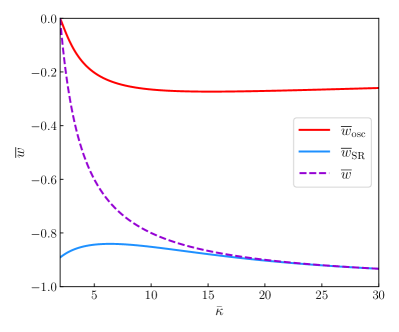
Figure 4: The stasis equation-of-state parameters ${\overline{w}}_{\rm SR}$ and ${\overline{w}}_{\rm osc}$ for our slow-roll and oscillatory energy components, along with the equation-of-state parameter ${\overline{w}}$ for the tower of scalar fields as a whole, plotted as functions of the parameter ${\overline{\kappa}}$ within the range $2\leq{\overline{\kappa}}\leq 30$.

The abundance ${\overline{\Omega}}_{\rm SR}$ of the slow-roll component during stasis can be obtained by applying the constraint in Eq. (39) to the expression in Eq. (38). Noting that $\rho_{0}^{(0)}=m_{0}^{2}(\phi_{0}^{(0)})^{2}/2$, we may express this abundance as

$${\overline{\Omega}}_{\rm SR}~{}=~{}\frac{\rho_{\rm SR}}{3M_{P}^{2}H^{2}}~{}=~{}\frac{3}{2}\frac{I_{\rm SR}^{(\rho)}({\overline{\kappa}})}{\delta{\overline{\kappa}}^{2}\mathcal{J}({\overline{\kappa}})}\left(\frac{m_{0}}{\Delta m}\right)^{1/\delta}\left(\frac{\phi_{0}^{(0)}}{M_{P}}\right)^{2}\,.$$ (48)

Thus, we find that ${\overline{\Omega}}_{\rm SR}$ exhibits an explicit dependence on the initial value of the lightest field in the tower.

Alternatively, ${\overline{\Omega}}_{\rm SR}$ may also be expressed in terms of the ratio $H^{(0)}/m_{N-1}$ of the initial value of the Hubble parameter to the mass of the heaviest scalar in the tower — a ratio which carries information the extent to which this scalar is damped at $t=t^{(0)}$. Indeed, in the continuum limit, one finds that the total initial abundance of the tower is given by

$$\Omega_{\rm tow}^{(0)}~{}=~{}\frac{m_{N-1}^{2}}{2\delta m_{0}^{2}}\left(\frac{m_{0}}{\Delta m}\right)^{1/\delta}\Omega_{0}^{(0)}\,$$ (49)

and that the initial energy density $\rho_{0}^{(0)}=3M_{P}^{2}(H^{(0)})^{2}\Omega_{0}^{(0)}$ of the lightest state in the tower may therefore be expressed as

$$\rho_{0}^{(0)}~{}=~{}6\delta\left(\frac{M_{P}H^{(0)}m_{0}}{m_{N-1}}\right)^{2}\left(\frac{\Delta m}{m_{0}}\right)^{1/\delta}\Omega_{\rm tow}^{(0)}\,.$$ (50)

Substituting this expression for $\rho_{0}^{(0)}$ into Eq. (38) and applying the constraint in Eq. (39), we obtain

$${\overline{\Omega}}_{\rm SR}~{}=~{}\frac{18I_{\rm SR}^{(\rho)}({\overline{\kappa}})}{{\overline{\kappa}}^{2}\mathcal{J}({\overline{\kappa}})}\left(\frac{H^{(0)}}{m_{N-1}}\right)^{2}\Omega_{\rm tow}^{(0)}\,.$$ (51)

Likewise, we note that the stasis abundance for the oscillatory component is given by

$${\overline{\Omega}}_{\rm osc}~{}=~{}\frac{18I_{\rm osc}^{(\rho)}({\overline{\kappa}})}{{\overline{\kappa}}^{2}\mathcal{J}({\overline{\kappa}})}\left(\frac{H^{(0)}}{m_{N-1}}\right)^{2}\Omega_{\rm tow}^{(0)}\,.$$ (52)

Taken together, Eqs. (48) and (51) imply that

$$\frac{H^{(0)}}{m_{N-1}}\sqrt{\Omega^{(0)}_{\rm tow}}~{}=~{}\sqrt{\frac{1}{12\delta}}\left(\frac{m_{0}}{\Delta m}\right)^{1/(2\delta)}\frac{\phi_{0}^{(0)}}{M_{P}}\,,$$ (53)

for any value of $m_{N-1}$. Indeed, straightforward calculation confirms that this relation holds even in the $m_{N-1}\to\infty$ limit, and that ${\overline{\Omega}}_{\rm SR}$ therefore remains finite in this limit as well. For a given aggregate initial abundance ${\overline{\Omega}}_{\rm tow}^{(0)}$ for the tower, then, we may treat ${\overline{\Omega}}_{\rm SR}$ as a function of two dimensionless parameters: ${\overline{\kappa}}$ and either $H^{(0)}/m_{N-1}$ or $\phi_{0}^{(0)}/M_{P}$.

Thus, to summarize the results of this section, we have shown that as long as the condition in Eq. (39) is satisfied, the system of dynamical equations which govern the evolution of our $\phi_{\ell}$ in the early universe permits a stasis solution wherein the aggregate abundances $\Omega_{\rm SR}$ and $\Omega_{\rm osc}$ both remain effectively constant. Somewhat miraculously, such a stasis solution emerges despite the fact that the equation-of-state parameters $w_{\ell}$ for the individual $\phi_{\ell}$ evolve non-trivially with time as each such field transitions dynamically from the overdamped to the underdamped phase. Of course, many approximations were made on the road to the result in Eq. (39). These include, for example, the transition to a continuum limit in Eq. (33) and the subsequent approximations for the summation endpoints in Eq. (34). However, it turns out that none of these approximations affect the manner in which our expression for $\Omega_{\rm SR}$ in Eq. (38) and the analogous expression for $\Omega_{\rm osc}$ depend on $t$. As a result, the constraint which cancels this time dependence — namely that in Eq. (39) — is an exact constraint that does not require any modification. Indeed, these approximations only affect the prefactors that are associated with these expressions, and we shall see that these prefactors are of lesser concern because changes to their precise values disturb neither the existence of the stasis state nor the ability of the universe to evolve into it. These issues are discussed more fully in Ref. Dienes et al. (2024).

It is interesting to compare the stasis condition for this system to the stasis condition derived in Ref. Dienes et al. (2024) for an analogous system consisting of a tower of $\phi_{\ell}$ states undergoing underdamping transitions in which each of the $\phi_{\ell}$ was modeled as having a fixed common equation-of-state parameter $w_{\ell}=w$ prior to the instant at which the critical-damping transition occurs and as having a fixed equation-of-state parameter $w_{\ell}=0$ thereafter. Taking the $w\to-1$ limit in this system would then correspond to treating each $\phi_{\ell}$ as pure vacuum energy prior to its underdamping transition and to treating each $\phi_{\ell}$ after as pure matter afterwards. For general values of $w$ lying within the range $-1<w<0$, it was then found that the condition for stasis is Dienes et al. (2024)

$$\alpha+\frac{1}{\delta}~{}=~{}2-(1+w){\overline{\kappa}}~{}.$$ (54)

Comparing this result with that in Eq. (39), we see that these two stasis conditions coincide precisely when $w=-1$. This then lends credence to both approaches to studying such towers of dynamical scalars and indicates that they are mutually consistent in the $w\to-1$ limit, which corresponds to a true vacuum-energy/matter stasis.

That said, there is an important fundamental difference between the results in Eqs. (39) and (54): given an input value for $\alpha+1/\delta$, the former constraint does not predict a particular stasis value for ${\overline{\kappa}}$ (or equivalently for $\overline{w}$), while the latter does. Or, phrased somewhat differently, our derivation of the stasis condition in Eq. (39) made absolutely no assumption concerning what other energy components might also simultaneously exist in the universe, so long as the entire universe experiences a net stasis with the Hubble parameter taking the form $H(t)\approx{\overline{\kappa}}/(3t)$ for some constant ${\overline{\kappa}}$. In particular, it was not necessary to impose any relationship between the value of ${\overline{\kappa}}$ and the abundances ${\overline{\Omega}}_{\rm SR}$ and ${\overline{\Omega}}_{\rm osc}$ — or equivalently between the total energy density $\rho_{\rm tot}$ of the universe and the contributions to $\rho_{\rm tot}$ which come from the tower states $\phi_{\ell}$ alone. We shall find in Sect. IV that this fundamental difference has profound consequences.

III.4 Stasis in a tower-dominated universe

Throughout this section, we have utilized the fact that the Hubble parameter during stasis takes the general form $H={\overline{\kappa}}/(3t)$. However, up to this point, we have made no assumptions concerning the value of ${\overline{\kappa}}$. In general, ${\overline{\kappa}}$ is directly related to the stasis value ${\overline{w}}_{\rm univ}$ of the equation-of-state parameter $w_{\rm univ}$ for the universe as a whole. In order to show this, we begin by noting that we can implicitly define a time-dependent parameter $\kappa(t)$ via the relation

$$\frac{dH}{dt}~{}=~{}-\frac{3}{\kappa}H^{2}~{}.$$ (55)

Indeed, during a stasis epoch in which $\kappa(t)$ is effectively constant with a value ${\overline{\kappa}}$, we recover from Eq. (55) the stasis relation $H\approx{\overline{\kappa}}/(3t)$. However, the Friedmann acceleration equation for a flat universe generally tells us

$$\frac{dH}{dt}~{}=~{}-\frac{3}{2}H^{2}\left(1+{w}_{\rm univ}\right)~{}.$$ (56)

Comparing Eqs. (55) and (56) then yields the general relation $\kappa=2/(1+w_{\rm univ})$, where $\kappa$ and $w_{\rm univ}$ are in general both time-dependent quantities. During stasis, both of these quantities are effectively constant and we therefore have

$${\overline{\kappa}}~{}=~{}\frac{2}{1+{\overline{w}}_{\rm univ}}\,.$$ (57)

While Eq. (57) provides a general relation between ${\overline{\kappa}}$ and ${\overline{w}}_{\rm univ}$, both of which describe the universe as a whole, we have not yet asserted any relation between these quantities and quantities such as $\overline{w}$ or ${\overline{\Omega}}_{\rm tow}$ which describe the tower itself. In other words, we have made no assumption about whether our scalar tower constitutes the entirety of the energy density of the universe, or whether there exist additional energy components during stasis as well. Such an assumption — and additional details concerning the abundances and equation-of-state parameters of any such energy components — would be necessary before any such relation between ${\overline{\kappa}}$ and $\overline{w}_{\rm univ}$ on the one hand, and quantities such as $\overline{w}$ and ${\overline{\Omega}}_{\rm tow}$ on the other hand, could be formulated. Thus, in order to proceed further, we must specify whether any additional energy components are present during stasis and what their properties might be.

For the remainder of this section, we shall focus on the simplest case — that in which the tower states collectively represent the entirety of the energy density in the universe. In other words, we shall assume that $\Omega_{\rm tow}(t)=1$ for all $t$ and defer our study of the more general case in which additional cosmological energy components are present to Sect. IV.

In the absence of additional energy components, we have ${\overline{\Omega}}_{\rm osc}=1-{\overline{\Omega}}_{\rm SR}$. Likewise, the equation-of-state parameter for the universe as a whole during stasis is simply ${\overline{w}}_{\rm univ}={\overline{w}}$, where in this case

$${\overline{w}}~{}=~{}{\overline{w}}_{\rm SR}{\overline{\Omega}}_{\rm SR}+{\overline{w}}_{\rm osc}{\overline{\Omega}}_{\rm osc}\,.$$ (58)

It therefore follows from Eq. (57) that

$${\overline{\kappa}}~{}=~{}\frac{2}{1+{\overline{w}}_{\rm osc}({\overline{\kappa}})+[{\overline{w}}_{\rm SR}({\overline{\kappa}})-{\overline{w}}_{\rm osc}({\overline{\kappa}})]{\overline{\Omega}}_{\rm SR}}\,,$$ (59)

where we have included the explicit dependence of ${\overline{w}}_{\rm SR}$ and ${\overline{w}}_{\rm osc}$ on ${\overline{\kappa}}$ in this expression in order to emphasize that these quantities not only depend on, but are indeed completely specified by, the value of ${\overline{\kappa}}$. Substituting the expression for ${\overline{\Omega}}_{\rm SR}$ in Eq. (51) with $\Omega^{(0)}_{\rm tow}=1$ into this equation, we arrive at a transcendental equation for ${\overline{\kappa}}$. This equation, which takes the form

$$\frac{2{\overline{\kappa}}-[1+{\overline{w}}_{\rm osc}({\overline{\kappa}})]{\overline{\kappa}}^{2}}{{\overline{w}}_{\rm SR}({\overline{\kappa}})-{\overline{w}}_{\rm osc}({\overline{\kappa}})}\,=\,\frac{18I_{\rm SR}^{(\rho)}({\overline{\kappa}})}{\mathcal{J}({\overline{\kappa}})}\left(\frac{H^{(0)}}{m_{N-1}}\right)^{2}\,,$$ (60)

may be solved numerically for any given value of the ratio $H^{(0)}/m_{N-1}$. From this solution, the corresponding values of ${\overline{\Omega}}_{\rm SR}$, ${\overline{\Omega}}_{\rm osc}$, ${\overline{w}}_{\rm SR}$, and ${\overline{w}}_{\rm osc}$ may be obtained in a straightforward manner.

In Fig. 5, we show both the value of ${\overline{\kappa}}$ (upper panel) and the values of ${\overline{\Omega}}_{\rm SR}$ and ${\overline{\Omega}}_{\rm osc}$ (lower panel) as functions of $H^{(0)}/m_{N-1}$. We observe from the upper panel that ${\overline{\kappa}}$ approaches the value ${\overline{\kappa}}=2$ associated with a matter-dominated universe in the $H^{(0)}/m_{N-1}\rightarrow 0$ limit, but grows without bound as $H^{(0)}/m_{N-1}$ increases. Accordingly, we observe from the lower panel that ${\overline{\Omega}}_{\rm SR}\rightarrow 0$ in the $H^{(0)}/m_{N-1}\rightarrow 0$ limit. However, this abundance increases monotonically with $H^{(0)}/m_{N-1}$ and approaches unity as $H^{(0)}/m_{N-1}\rightarrow\infty$.

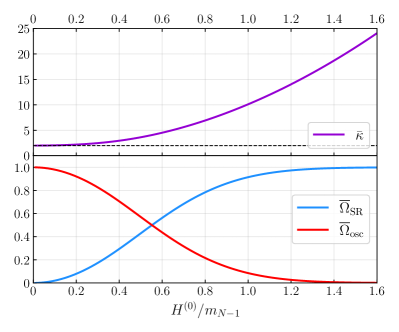
Figure 5: The value of ${\overline{\kappa}}$ (upper panel) and the values of ${\overline{\Omega}}_{\rm SR}$ and ${\overline{\Omega}}_{\rm osc}$ (lower panel), plotted as functions of the ratio $H^{(0)}/m_{N-1}$ for the case in which no additional energy components are present during stasis.

III.5 Dynamical evolution and attractor behavior

Having established the conditions under which stasis can emerge in our dynamical-scalar scenario, and having determined how the stasis abundances ${\overline{\Omega}}_{\rm SR}$ and ${\overline{\Omega}}_{\rm osc}$ depend on input parameters, we now examine whether $\Omega_{\rm SR}$ and $\Omega_{\rm osc}$ in fact evolve dynamically toward these stasis values, given the initial conditions we have specified for the $\phi_{\ell}$. We shall perform our analysis of the cosmological dynamics by numerically solving the coupled system of equations of motion for $H$ and $\phi_{\ell}$. For the moment, we shall focus on the case in which $\Omega_{\rm tow}(t)=1$ for all $t$ and defer discussion of the more general case until Sect. IV.

In the upper panel of Fig. 6, we plot the abundances $\Omega_{\rm SR}(t)$ of the slow-roll component (solid curves) as functions of the dimensionless time variable $m_{0}t$ for $H^{(0)}/m_{N-1}=\{0.23,0.40,0.55,0.71,0.97\}$. The corresponding stasis abundances — obtained from Eq. (51) with $\Omega_{\rm tow}^{(0)}=1$ and with ${\overline{\kappa}}$ determined implicitly through Eq. (60) — are respectively given by ${\overline{\Omega}}_{\rm SR}=\{0.1,0.3,0.5,0.7,0.9\}$. For each $\Omega_{\rm SR}$ curve shown, the dotted horizontal line of the same color indicates the corresponding value of ${\overline{\Omega}}_{\rm SR}$. By contrast, in the lower panel of Fig. 6, we plot the corresponding equation-of-state parameters $\langle w\rangle(t)$ for the tower as a whole (solid curves) as functions of $m_{0}t$. For each $\langle w\rangle$ curve shown, the dotted horizontal line of the same color indicates the corresponding value of ${\overline{w}}_{\rm SR}$. All of the curves shown in Fig. 6 correspond to the parameter choices $\alpha=1$ and $\delta=1$.

We see from Fig. 6 that the universe evolves dynamically toward stasis regardless of the initial value $H^{(0)}/m_{N-1}$. However, consistent with our result in Eq. (51), we see that the particular stasis value ${\overline{\Omega}}_{\rm SR}$ towards which $\Omega_{\rm SR}$ evolves does depend on this ratio. We also see from this figure that the universe can remain in stasis, with an effectively fixed abundance ${\overline{\Omega}}_{\rm SR}$, for a significant duration, even for a moderate value of $N$. Indeed, the curves shown in Fig. 6 were calculated with $N=5000$, and even with this relatively small value the stases shown in Fig. 6 have not yet reached their endpoints. We shall discuss the relationship between $N$ and the resulting number of $e$-folds of stasis below.

We emphasize that while certain quantitative aspects of the $\Omega_{\rm SR}$ curves shown in Fig. 6 reflect the particular values of $\alpha$ and $\delta$ we have chosen, the abundance curves obtained for other combinations of $\alpha$ and $\delta$ which likewise satisfy the stasis condition in Eq. (39) are qualitatively similar. Indeed, we find that the universe is generically attracted toward stasis in each case, despite the fact that ${\overline{\Omega}}_{\rm SR}$ depends on $H^{(0)}/m_{N-1}$.

More generally, we find that the universe is always attracted towards a stasis solution within this dynamical-scalar system regardless of the initial conditions. The initial conditions affect the values of the abundances and equation-of-state parameters of our cosmological energy components during stasis, but the universe is always attracted towards a stasis configuration.

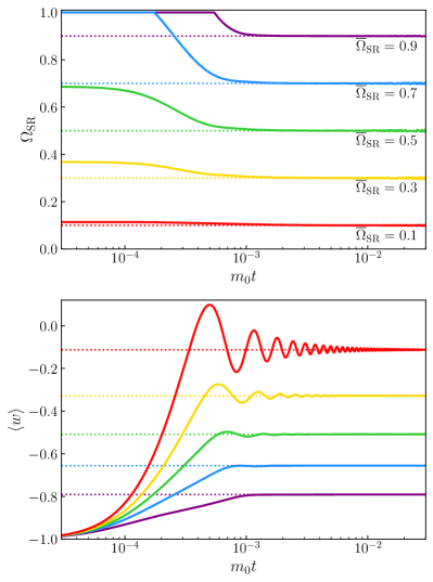
Figure 6: Upper panel: The abundances $\Omega_{\rm SR}(t)$ of the slow-roll energy component (solid curves), plotted as functions of the dimensionless time variable $m_{0}t$ for $H^{(0)}/m_{N-1}=\{0.23,0.40,0.55,0.71,0.97\}$. These values of $H^{(0)}/m_{N-1}$ respectively correspond to the stasis abundances ${\overline{\Omega}}_{\rm SR}=\{0.1,0.3,0.5,0.7,0.9\}$. For each curve, the dotted horizontal line of the same color indicates the corresponding value of ${\overline{\Omega}}_{\rm SR}$. Lower panel: The effective equation-of-state parameters $\langle w\rangle(t)$ for the scalar tower as a whole (solid curves), plotted as functions of $m_{0}t$ over the same range as in the upper panel. Each curve corresponds to the same value of $H^{(0)}/m_{N-1}$ as the curve of the same color in the upper panel. For each curve, the dotted horizontal line indicates the corresponding value of ${\overline{w}}_{\rm SR}$. All of the results shown in either panel correspond to the parameter choices $\alpha=1$ and $\delta=1$.

Since we are assuming that $\dot{\phi}_{\ell}^{(0)}=0$ for all fields in the tower, we initially have $\left\langle w\right\rangle=-1$, regardless of the value of $H^{(0)}/m_{N-1}$. Moreover, as the system evolves toward stasis, we also observe that $\left\langle w\right\rangle$ approaches the constant value ${\overline{w}}$ obtained from Eq. (43) with ${\overline{\kappa}}$ determined explicitly through Eq. (60). In cases in which the initial value of $\Omega_{\rm osc}=1-\Omega_{\rm SR}$ is relatively large, we observe that the value of $\left\langle w\right\rangle$ oscillates around ${\overline{w}}_{\rm SR}$ before it settles into its stasis value. This is due to the fact that the highly oscillatory $\phi_{\ell}$ have a more significant impact on the value of $\langle w\rangle$ when $\Omega_{\rm osc}$ is large. Indeed, this oscillatory behavior is less pronounced when $\Omega_{\rm SR}$ is relatively large and the contribution to $\left\langle w\right\rangle$ from $\Omega_{\rm osc}w_{\rm osc}$ is therefore less significant.

As is the case with ${\overline{\Omega}}_{\rm SR}$ and ${\overline{w}}$, we find that the duration of the stasis epoch — and therefore the number $\mathcal{N}_{s}$ of $e$-folds of expansion the universe undergoes during this epoch — depends on the ratio $H^{(0)}/m_{N-1}$. In the regime in which $3H^{(0)}>2m_{N-1}$ and all of the $\phi_{\ell}$ are effectively underdamped at $t=t^{(0)}$, we may obtain a rough estimate for $\mathcal{N}_{s}$ by approximating the duration of the stasis epoch to be the interval between the times $t_{N-1}$ and $t_{0}$ at which $\phi_{N-1}$ and $\phi_{0}$ undergo their critical-damping transitions, respectively. Approximating $H\approx{\overline{\kappa}}/(3t)$ at each of these transition times and using the fact that the scale factor scales like $a\sim t^{{\overline{\kappa}}/3}$ during stasis, we find that

$$\mathcal{N}_{s}~{}\approx~{}\log\left[\frac{a(t_{0})}{a(t_{N-1})}\right]~{}\approx~{}\frac{{\overline{\kappa}}}{3}\log\left[\frac{t_{0}}{t_{N-1}}\right]\,.$$ (61)

By contrast, in the opposite regime, in which $3H^{(0)}<2m_{N-1}$, all $\phi_{\ell}$ with masses $m_{\ell}>3H^{(0)}/2$ would begin oscillating immediately at $t=t^{(0)}$. In this regime, then, $\mathcal{N}_{s}$ is given by a expression similar to that in Eq. (61), but with $t_{N-1}\rightarrow t^{(0)}$. As a result, in either regime, we have

$$\mathcal{N}_{s} \approx \frac{{\overline{\kappa}}}{3}\log\left(\frac{t_{0}}{\max\{t_{N-1},t^{(0)}\}}\right)$$ (62)

$$\approx \frac{{\overline{\kappa}}}{3}\Bigg{[}\delta\log N+\log\left(\frac{\Delta m}{m_{0}}\right)$$

$$~{}~{}~{}~{}+\log\left(\frac{3H^{(0)}}{\max\{3H^{(0)},2m_{N-1}\}}\right)\Bigg{]}\,.~{}~{}~{}~{}~{}~{}$$

We see from Eq. (62) that $\mathcal{N}_{s}$ increases logarithmically with the number of $\phi_{\ell}$ in the tower. Moreover, we also see that $\mathcal{N}_{s}$ increases monotonically with the ratio $H^{(0)}/m_{N-1}$ for a given choice of $m_{0},\Delta m,\delta$, and $N$. This is due primarily to the fact that ${\overline{\kappa}}$ likewise increases monotonically with this ratio, but the growth of $\mathcal{N}_{s}$ with $H^{(0)}/m_{N-1}$ is also enhanced in the $H^{(0)}/m_{N-1}<2/3$ regime due to the fact that all $\phi_{\ell}$ with $m_{\ell}>3H^{(0)}/2$ begin oscillating immediately at $t=t^{(0)}$.

We note, however, that the expression in Eq. (62) overestimates the value of $\mathcal{N}_{s}$ within the regime in which $\delta$ is small and the ratio $m_{0}/\Delta m$ is non-negligible. Within this regime, the mass spectrum of the $\phi_{\ell}$ is significantly compressed and the value of $m_{0}$ therefore has a non-negligible impact on the $m_{\ell}$ across a significant portion of the tower. As a result, although our fundamental scaling relation between $m_{\ell}$ and $\ell$ in Eq. (23) continues to hold, this relation is no longer well approximated by the simpler power-law relation $m_{\ell}/\Delta m\approx\ell^{\delta}$ within this portion of the tower. Thus, the manner in which the $\phi_{\ell}^{(0)}$ scale with $\ell$ deviates significantly from the scaling relation in Eq. (40). Thus, while the universe evolves toward and subsequently remains in stasis as long as the total energy density of the tower remains dominated by $\phi_{\ell}$ with $m_{\ell}\gg m_{0}$, the stasis epoch effectively ends as soon as the lighter $\phi_{\ell}$ whose $\phi_{\ell}^{(0)}$ do not satisfy this scaling relation begin to dominate that total energy density. That said, in the opposite regime, in which $m_{0}\ll\Delta m$, the $\phi^{(0)}_{\ell}$ satisfy this scaling relation across essentially the entire tower, and the expression in Eq. (62) still furnishes a reasonable estimate for $\mathcal{N}_{s}$.

III.6 Alternative partitions

Before moving forward, we comment on one additional property of our realization of stasis which bears mention. The two cosmological energy components which coexist with constant abundances during stasis — components which we have called “slow-roll” and “oscillatory” — are each derived from collections of fields whose individual equation-of-state parameters evolve continuously from $w_{\ell}=-1$ to $w_{\ell}=0$. As indicated in Sect. III.1, the criterion we have adopted in order to determine with which energy component a given such field should be associated at any particular time $t$ is whether or not $3H(t)\geq 2m_{\ell}$. If this criterion is satisfied for a given $\phi_{\ell}$, we associate this field with the slow-roll component; if it is not, we associate this field with the oscillatory component. This is certainly a physically motivated choice, given that it associates all $\phi_{\ell}$ which are overdamped at time $t$ with the slow-roll component and all of the fields which are underdamped with the oscillatory component.

While the distinction between overdamped and underdamped fields is a mathematically important one, there is nevertheless no sharp distinction that occurs in the behavior of a given field as it crosses this boundary. Even for a single scalar field evolving in a fixed external cosmology, as shown in Fig. 1, the transition from the overdamped to underdamped regimes is a completely smooth one. For this reason, it is natural to wonder whether our discovery of a stasis between the slow-roll and oscillatory components critically relies on this being taken as the definitional boundary between the two components, or whether an analogous stasis might exist even if this boundary were shifted in either direction.

As we shall now see, a stasis emerges even if this boundary is shifted. More specifically, if we were to replace our standard “slow-roll” criterion $3H(t)\geq 2m_{\ell}$ with a generalized criterion

$$3\,A\,H(t)~{}\geq~{}2\,m_{\ell}~{}$$ (63)

where $A$ is an arbitrary positive constant, we would find that a stasis develops regardless of the value of $A$. Such a stasis would then take place between the abundances of the new “slow-roll” component (i.e., now defined as the component comprising fields which satisfy this modified criterion at time $t$) and the new “oscillatory” component (i.e., the component comprising fields which do not).

It is straightforward to understand why such a stasis continues to arise. Since the upper limit of integration in Eq. (36) is given by $m_{\ell_{c}}=3AH/2=A{\overline{\kappa}}/(2t)$ for such a criterion, it follows that $I^{(\rho)}_{\rm SR}({\overline{\kappa}})$ is likewise independent of $t$ for any choice of $A$ and given by

$$I^{(\rho)}_{\rm SR}({\overline{\kappa}})~{}=~{}\int_{0}^{A{\overline{\kappa}}/2}d\tilde{t}~{}\tilde{t}^{\alpha+1/\delta-{\overline{\kappa}}}\left[J_{\frac{{\overline{\kappa}}+1}{2}}^{2}(\tilde{t})+J_{\frac{{\overline{\kappa}}-1}{2}}^{2}(\tilde{t})\right]\,.$$ (64)

The corresponding expressions for the quantity $I^{(P)}_{\rm SR}({\overline{\kappa}})$ Eq. (41) and for the quantities $I^{(\rho)}_{\rm osc}({\overline{\kappa}})$ and $I^{(P)}_{\rm osc}({\overline{\kappa}})$ are obtained by making the replacement ${\overline{\kappa}}/2\rightarrow A{\overline{\kappa}}/2$ in the upper and lower limits of integration, respectively. Since since $I^{(\rho)}_{\rm SR}({\overline{\kappa}})$ and $I^{(\rho)}_{\rm osc}({\overline{\kappa}})$ are both constant during stasis for any choice of the partition parameter $A$, the corresponding abundances $\Omega_{\rm SR}$ and $\Omega_{\rm osc}$ are likewise constant during stasis whenever Eq. (39) is satisfied. Moreover, while the particular values ${\overline{\Omega}}_{\rm SR}$ and ${\overline{\Omega}}_{\rm osc}$ that these abundances take during stasis do depend non-trivially on $A$, we find that $\Omega_{\rm SR}$ and $\Omega_{\rm osc}$ evolve dynamically toward these stasis values for any choice of this partition parameter.

In Fig. 7, we plot the stasis abundances ${\overline{\Omega}}_{\rm SR}$ and ${\overline{\Omega}}_{\rm osc}$ as functions of $A$ for the parameter choice $H^{(0)}/m_{N-1}=2/3$. For reference, we also include a dotted vertical line indicating our usual value $A=1$, which corresponds to choosing the partition location to coincide with the location of the underdamping transition. As we see from this figure, the effect of increasing $A$ is to increase ${\overline{\Omega}}_{\rm SR}$ and to decrease ${\overline{\Omega}}_{\rm osc}$, with the opposite results arising for decreasing $A$. It is easy to understand this behavior. Let us imagine increasing the value of $A$ during stasis. This then effectively increases the critical value $\ell_{c}(t)$ of $\ell$ for which the criterion $3AH(t)\geq 2m_{\ell}$ is satisfied at any given time. This in turn has the effect of shifting certain $\phi_{\ell}$ states from the set of states which contribute to ${\overline{\Omega}}_{\rm osc}$ to the set of states contributing to ${\overline{\Omega}}_{\rm SR}$. This causes the former abundance to decrease and the latter abundance to increase. Moreover, this effect is never washed out at subsequent times because we are in stasis. Thus the new re-partitioned abundances are fixed and do not evolve further.

Although we have seen that a stasis emerges over a wide range of values for $A$, there are intrinsic limits to how large or small $A$ may be taken. Indeed, these limits can be seen in Fig. 7: when $A$ is taken too large, ${\overline{\Omega}}_{\rm osc}$ falls to zero, while if $A$ is taken too small, ${\overline{\Omega}}_{\rm SR}$ falls to zero. Thus, in either extreme limit, we no longer obtain a meaningful stasis between two significant energy components. We can also understand this behavior by thinking about the $\phi_{\ell}$ tower. Given that we have posited a tower of $N$ components, it is possible for the value of $A$ to become so large or so small that we have either too few states in the oscillatory phase at the top of the tower at early times or too few states in the slow-roll phase at the bottom of the tower at late times. In either case, the prevalence of such significant “edge” effects can then prevent a stasis from developing at early times or surviving until late times. These destructive effects arise because the existence of too few states in either scenario would invalidate some the approximations (such as the continuum approximation) that were made in Sect. III.  This then seriously curtails (or potentially even completely eliminates) the length of time available for a corresponding stasis epoch. However, as long as $A$ is not taken to these extremes, we see that we have a healthy stasis whose existence persists regardless of changes in $A$.

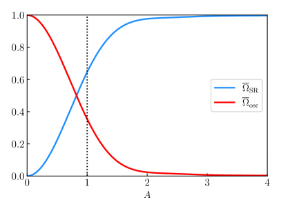
Figure 7: The stasis abundances ${\overline{\Omega}}_{\rm SR}$ and ${\overline{\Omega}}_{\rm osc}$ that emerge for arbitrary choices of the partition parameter $A$ in Eq. (63), plotted as functions of $A$ for the reference value $H^{(0)}/m_{N-1}=2/3$. The vertical line indicates the standard choice $A=1$ that we have made throughout this paper. We see that a stasis emerges for all values of $A$ shown, with the resulting stasis abundances increasingly favoring ${\overline{\Omega}}_{\rm SR}$ for larger $A$ and ${\overline{\Omega}}_{\rm osc}$ for smaller $A$.

Thus far we have focused on the partitioning of our tower into only two energy components. However, we can even consider a more general partitioning of the tower into a an arbitrary number $N_{C}$ of cosmological energy components. These components may be labeled by an index $i=1,2,\ldots,N_{C}$. We define an abundance $\Omega_{i}$ and a partition parameter $A_{i}$ for each of these energy components such that $A_{1}=0$ and $A_{i+1}>A_{i}$. For all $i<N_{C}$, we associate the abundances $\Omega_{\ell}$ of all of the $\phi_{\ell}$ with masses within the range $3A_{i+1}H(t)\geq 2m_{\ell}>3A_{i}H(t)$ with $\Omega_{i}$. We associate the abundances $\Omega_{\ell}$ of all the $\phi_{\ell}$ with masses $2m_{\ell}>3A_{N_{C}}H(t)$ with $\Omega_{N_{C}}$.

For such a general partition, we find that when the condition in Eq. (39) is satisfied, a stasis — one in which all of the $\Omega_{i}$ take effectively constant values — likewise emerges in the continuum limit. These stasis abundances ${\overline{\Omega}}_{i}$ are given by functions of the form in Eq. (48) with $I^{(\rho)}_{\rm SR}({\overline{\kappa}})$ replaced by a function of the form

$$I^{(\rho)}_{i}({\overline{\kappa}})~{}=~{}\int^{A_{i+1}{\overline{\kappa}}/2}_{A_{i}{\overline{\kappa}}/2}d\tilde{t}~{}\tilde{t}^{\alpha+1/\delta-{\overline{\kappa}}}\left[J_{\frac{{\overline{\kappa}}+1}{2}}^{2}(\tilde{t})+J_{\frac{{\overline{\kappa}}-1}{2}}^{2}(\tilde{t})\right]$$ (65)

for $i<N_{C}$, and by a similar expression with the replacement $A_{i+1}{\overline{\kappa}}/2\rightarrow\infty$ in upper limit of integration for $i=N_{C}$. We also find numerically that the $\Omega_{i}$ are dynamically attracted toward their corresponding ${\overline{\Omega}}_{i}$ values for arbitrary such partitionings of the tower into energy components.

We see, then, that the emergence of stasis from a tower of dynamical scalars does not depend on the manner in which we partition the tower into energy components based on the relationships between $H(t)$ and the individual $m_{\ell}$. That said, the two-component partition which we have been employing thus far in this paper, in which one component comprises the scalars which are overdamped at any given time and the other comprises the scalars which are underdamped, is a physically meaningful one, and we shall continue to adopt this partition in what follows.

IV Stasis in the presence of a background energy component

In this section we investigate what happens if we repeat our previous analysis, only now in the presence of an additional energy component which we may regard as a “background spectator” — i.e., a fluid which is completely inert, neither receiving energy from our $\phi_{\ell}$ fields nor donating energy to them. We shall conduct our analysis in two stages. First, we will consider the case in which this background is time-independent, with a fixed equation-of-state parameter $w_{\rm BG}$. We shall then consider how our results are modified if our background has a time-dependent equation-of-state parameter $w_{\rm BG}(t)$.

IV.1 Time-independent background

We begin our analysis by considering the case in which our background fluid has a fixed equation-of-state parameter $w_{\rm BG}$. We shall make no other assumptions regarding the nature of this background and we shall allow its initial abundance $\Omega^{(0)}_{\rm BG}$ to be completely arbitrary. Thus, even though we shall refer to this energy component as a “background”, we shall not assume that it dominates the cosmology of our system.

In the following analysis, we shall let $\overline{w}$ represent the equation-of-state parameter of our dynamical-scalar system during the stasis that would have resulted if there had been no extra background component. Indeed, $\overline{w}$ will continue to be given by Eq. (58) where ${\overline{\Omega}}_{\rm SR}$ and ${\overline{\Omega}}_{\rm osc}$ are likewise the values of $\Omega_{\rm SR}$ and $\Omega_{\rm osc}$ that would have emerged in such a background-free stasis. As long as our slow-roll and oscillatory components have reached stasis, all of the quantities in Eq. (58) are time-independent. We shall also continue to let $\langle w\rangle$ denote the time-dependent equation-of-state parameter for our $\phi_{\ell}$ tower alone, as in Eq. (19). By contrast, we shall let $w_{\rm univ}$ continue to denote the equation-of-state parameter for the entire universe, bearing in mind that this now includes not only the contribution from the $\phi_{\ell}$ tower but also the contribution from the background:

$$w_{\rm univ}~{}\equiv~{}\sum_{i}w_{i}\Omega_{i}~{}=~{}\langle w\rangle\,\Omega_{\rm tow}+w_{\rm BG}\,\Omega_{\rm BG}~{}.$$ (66)

Indeed, with this definition Eq. (57) continues to apply.

As we have already remarked at the end of Sect. III.3, we do not expect the existence of a stasis solution to be disturbed by the introduction of a background. However, what interests us here are the answers to two questions:

• How is the stasis solution affected by the presence of the spectator background?

• How is the dynamics of our system affected by the presence of the spectator background? Does the (possibly new) stasis solution continue to serve as an attractor?

In this section, we shall provide answers to these questions.

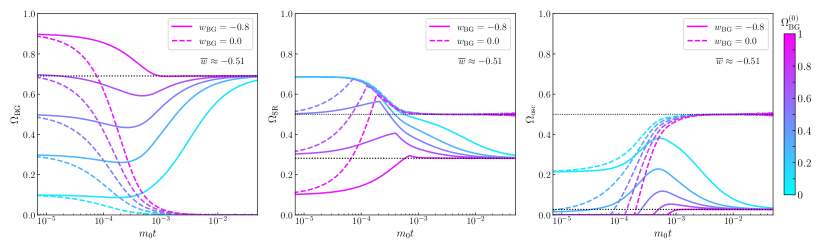
Figure 8: The time-evolution of the abundances $\Omega_{\rm BG}$ (left panel), $\Omega_{\rm SR}$ (middle panel), and $\Omega_{\rm osc}$ (right panel), plotted as functions of $m_{0}t$ for two different choices of the equation-of-state parameter $w_{\rm BG}$ for the background fluid (solid versus dashed lines). The differently colored lines represent different choices of the initial abundance $\Omega_{\rm BG}^{(0)}$ for this background fluid. The parameters chosen for these plots correspond to a system which would have had ${\overline{w}}=-0.51$ in the absence of the background fluid. In all cases, we see that the system evolves towards a stasis solution in which $\Omega_{\rm SR}$ and $\Omega_{\rm osc}$ have constant, non-zero values — values which are independent of $\Omega_{\rm BG}^{(0)}$ but nevertheless depend on the value of $w_{\rm BG}$. Indeed, for $w_{\rm BG}=0$ (dashed lines), we observe that $\Omega_{\rm BG}\to 0$ as time increases for all $\Omega_{\rm BG}^{(0)}$. By contrast, for $w_{\rm BG}=-0.8$ (solid lines), we find that $\Omega_{\rm BG}$ always asymptotes to a fixed non-zero value.

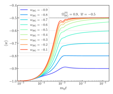
Figure 9: The effective equation-of-state parameter $\langle w\rangle$ for a tower with $\overline{w}=-0.5$, evaluated in the presence of a background fluid with equation-of-state parameter $w_{\rm BG}$ and plotted as a function of time for different fixed values of $w_{\rm BG}$. As we sweep through increasing values of $w_{\rm BG}$, we find that $\langle w\rangle$ always reaches a stasis value. For $w_{\rm BG}>\overline{w}$, we find that this stasis value saturates at $\overline{w}$. By contrast, for $w_{\rm BG}<\overline{w}$, we find that this stasis value is given by $w_{\rm BG}$. Thus, for $w_{\rm BG}<\overline{w}$, we see that the stasis equation-of-state parameter $\langle w\rangle$ for our system tracks that of the background.

We begin by investigating the effect that varying both the initial abundance $\Omega_{\rm BG}^{(0)}$ and equation-of-state parameter $w_{\rm BG}$ of the background has on the manner in which the abundances $\Omega_{\rm SR}$ and $\Omega_{\rm osc}$ evolve with time. In Fig. 8, we plot $\Omega_{\rm BG}$ (left panel), $\Omega_{\rm SR}$ (middle panel), and $\Omega_{\rm osc}$ as functions of $m_{0}t$ for several different combinations of $\Omega_{\rm BG}^{(0)}$ and $w_{\rm BG}$.

For all combinations of $\Omega_{\rm BG}^{(0)}$ and $w_{\rm BG}$, we observe that the universe evolves towards a stasis in which $\Omega_{\rm SR}$ and $\Omega_{\rm osc}$ have constant, non-zero values. In this three-component system, this of course implies that $\Omega_{\rm BG}$ evolves toward a constant value as well. Moreover, we observe that the value of $\Omega_{\rm BG}^{(0)}$ has no effect on the constant values toward which $\Omega_{\rm SR}$ and $\Omega_{\rm osc}$ ultimately evolve. Indeed, the stasis that emerges for a given choice of $w_{\rm BG}$ is also completely independent of $\Omega_{\rm BG}^{(0)}$. This is already an interesting result — one which confirms our expectation that the presence of a background component should affect neither the existence of a stasis solution within our dynamical system, nor the fact that this solution is an attractor within that system.

That said, we also see from Fig. 8 that the stasis which emerges in the presence of a background component depends non-trivially on the value of $w_{\rm BG}$. The results shown for the larger value of $w_{\rm BG}$ (dashed lines) indicate that $\Omega_{\rm BG}\to 0$ for all choices of $\Omega_{\rm BG}^{(0)}$. Furthermore, the stasis abundances which ultimately emerge for the slow-roll and oscillatory components after the background abundance dies away are precisely the same stasis abundances that we would have obtained for a slow-roll/oscillatory-component stasis with background absent altogether. By contrast, the results for the smaller value of $w_{\rm BG}$ (solid lines) indicate that $\Omega_{\rm BG}$ asymptotes toward a finite, non-zero value. Thus ${\overline{\Omega}}^{\prime}_{\rm SR}+{\overline{\Omega}}^{\prime}_{\rm osc}<1$ for the stasis that emerges, where ${\overline{\Omega}}_{\rm SR}^{\prime}$ and ${\overline{\Omega}}^{\prime}_{\rm osc}$ denote the modified stasis abundances for the slow-roll and oscillatory energy components which emerge in the presence of the background.

In order to further elucidate the manner in which ${\overline{\Omega}}_{\rm SR}^{\prime}$ and ${\overline{\Omega}}^{\prime}_{\rm osc}$ depend on $w_{\rm BG}$, in Fig. 9 we plot $\langle w\rangle$ as a function of $m_{0}t$ for a variety of different choices of $w_{\rm BG}$. All curves shown correspond to the parameter choices $\overline{w}=-0.5$ and $\Omega_{\rm BG}^{(0)}=0.9$. For $w_{\rm BG}<\overline{w}$, we find that the stasis value of $\langle w\rangle$ is given by $w_{\rm BG}$. By contrast, for $w_{\rm BG}>{\overline{w}}$, we find that this stasis value saturates at $\overline{w}$.

For $w_{\rm BG}>\overline{w}$, this latter result is easy to understand. As our system evolves, $\overline{w}$ is less than $w_{\rm BG}$. Thus our background redshifts away, i.e.,

$$\Omega_{\rm BG}~{}\to~{}0~{},$$ (67)

purely as a consequence of cosmological expansion. Indeed we have already seen this behavior within the dashed curves of the left panel of Fig. 8. Thus our system is ultimately attracted to the same stasis configuration as we would have had if the background had never been present, with $\Omega_{\rm SR}\to{\overline{\Omega}}_{\rm SR}$ and $\Omega_{\rm osc}\to{\overline{\Omega}}_{\rm osc}$. It is for this reason that $\langle w\rangle\to\overline{w}$. The stasis values for the abundances that emerge in this case are nothing but the values that are predicted by replacing $H^{(0)}$ with $H^{(0)}\sqrt{\Omega_{\rm tow}^{(0)}}$ in Eq. (60). In other words, we reproduce our original stasis that emerged in the absence of a background but with the same total initial energy density of the tower. This makes sense, since there is no background energy component remaining in the system. In such cases, the earlier period during which the background energy component still exists can then be viewed as a “pre-history” to the overall story.

By contrast, the manner in which the abundances behave for $w_{\rm BG}<\overline{w}$ is completely different. Within this regime, our background does not redshift away, and indeed $\Omega_{\rm BG}$ asymptotes to a non-zero stasis value. This means that $\Omega_{\rm SR}$ and $\Omega_{\rm osc}$ can no longer asymptote to the same stasis values that they would have had if no background had been present. In other words, in this case the presence of the background necessarily deforms the stasis away from what it would have been if the background had not been present. Remarkably, however, the new stasis that is realized is one wherein

$$\overline{w}^{\prime}~{}=~{}w_{\rm BG}~{},$$ (68)

where ${\overline{w}}^{\prime}$ denotes the modified value which $\langle w\rangle$ takes during stasis in the presence of the background. In other words, the new stasis that is realized in this case has an equation-of-state parameter which tracks that of the background! This tracking behavior occurs regardless of the initial abundance $\Omega_{\rm BG}^{(0)}$ of the background — indeed, the background need not even be dominant. Moreover, this behavior occurs regardless of the value that $w_{\rm BG}$ takes, so long as $w_{\rm BG}<\overline{w}$.

This, then, is our first example of a “tracking” stasis. As long as a background is present, and as long as $w_{\rm BG}<\overline{w}$ (so that this background survives into the stasis epoch without redshifting away), the modified equation-of-state parameter ${\overline{w}}^{\prime}$ for the tower will always match that of the background. If the initial background abundance $\Omega_{\rm BG}^{(0)}$ is large, this deformation of our stasis solution to match the background occurs relatively quickly. For smaller $\Omega_{\rm BG}^{(0)}$, by contrast, the deformation occurs more slowly. However, so long as $\Omega_{\rm BG}^{(0)}\not=0$, the abundances of the three cosmological energy components in our system will automatically reconfigure themselves such that ${\overline{w}}^{\prime}$ matches $w_{\rm BG}$.

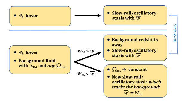
Figure 10: The cosmological evolution of a tower of scalar fields $\phi_{\ell}$ in the presence of a background with equation-of-state parameter $w_{\rm BG}$. Without the background (top row of figure), we have seen in Sect. III that our system naturally evolves into a slow-roll/oscillatory-component stasis with an equation-of-state parameter $\overline{w}$. Given this, the consequences of introducing the background (lower row of figure) depend on how $w_{\rm BG}$ relates to $\overline{w}$. If $w_{\rm BG}>\overline{w}$, the background simply redshifts away while the tower continues to produce the same slow-roll/oscillatory-component stasis as before. However, if $w_{\rm BG}<\overline{w}$, we find that $\Omega_{\rm BG}$ evolves towards a non-zero constant while the tower now evolves into a different stasis configuration wherein the modified equation-of-state parameter $\overline{w}^{\prime}$ is equal to $w_{\rm BG}$. In this way, then, the equation-of-state parameter for the tower during stasis tracks the background.

Given these observations, the cosmological evolution of a tower of scalar fields $\phi_{\ell}$ in the presence of a background fluid with equation-of-state parameter $w_{\rm BG}$ can be summarized as in Fig. 10. The top part of this figure indicates that our system without any background produces a stasis with a certain equation-of-state parameter $\overline{w}$. The lower part of the figure then illustrates that when the background is present, we obtain a stasis whose equation-of-state parameter is generally given by

$$\langle w\rangle~{}\to~{}\min\left\{\overline{w},\,w_{\rm BG}\right\}~{}.$$ (69)

Thus, for $w_{\rm BG}<\overline{w}$, we obtain Eq. (68).

This result makes perfect sense. In Ref. Dienes et al. (2022a) we demonstrated on general grounds that a pairwise stasis cannot exist in the presence of a spectator unless the two parts of the system — i.e., the tower of dynamical scalars and the background spectator — have the same effective equation-of-state parameter. It is thus the result in Eq. (68) that enables a stasis between the slow-roll and oscillatory components within the tower to arise even in the presence of the background spectator. Indeed, we see that the only way in which we can evade having $\overline{w}^{\prime}=w_{\rm BG}$ is to have $w_{\rm BG}<\overline{w}$. In that regime, the background spectator redshifts away, simply leaving us with $\overline{w}^{\prime}=\overline{w}$.

At this stage, several comments are in order. First, even though $\Omega_{\rm BG}$, $\Omega_{\rm SR}$, and $\Omega_{\rm osc}$ all asymptote to fixed, non-zero values for $w_{\rm BG}<\overline{w}$, it is important to note that this is not a triple stasis of the sort discussed in Ref. Dienes et al. (2024). Indeed, in this scenario, there is no transfer of energy between the background energy component and either $\rho_{\rm SR}$ and/or $\rho_{\rm osc}$. Rather, the behavior which our system exhibits for $w_{\rm BG}<\overline{w}$ exemplifies a possibility discussed in Ref. Dienes et al. (2022a), wherein which a pairwise stasis between two cosmological components takes place in the presence of a background component.

Second, we remark that it is only this slow-roll/oscillatory-component stasis achieved through dynamical scalars which has the ability to track a background. This does not happen for any realization of stasis previously identified in the literature, including the matter/radiation stasis outlined in Refs. Dienes et al. (2022a, b) or any of the pairwise stases — or even the triple stasis — discussed in Ref. Dienes et al. (2024). The underlying reason for this is actually quite simple. In all of these other realizations of stasis, the underlying constraint equations relate $\alpha+1/\delta$ directly to the value of the equation-of-state parameter ${\overline{w}}$ during stasis. For example, in the case of matter/radiation stasis achieved via towers of decaying matter fields Dienes et al. (2022a), our underlying constraint equation took the form

$$\frac{1}{\gamma}\left(\alpha+1/\delta\right)~{}=~{}2-{\overline{\kappa}}~{}=~{}\frac{2\overline{w}}{1+\overline{w}}~{}$$ (70)

where $\gamma$ is a parameter governing the scaling of decay widths $\Gamma_{\ell}$ across the tower and where ${\overline{\kappa}}=2/(1+\overline{w})$. Thus, once one specifies the fixed underlying parameters $(\alpha,\gamma,\delta)$ of our model, the resulting stasis value $\overline{w}$ is fixed and cannot be altered. This implies that if we introduce a spectator with equation-of-state parameter $w_{\rm BG}$ into such systems, and if $w_{\rm BG}$ differs from the value of ${\overline{w}}$ predicted from the constraint equations, there is no mechanism via which the value of ${\overline{w}}$ can be deformed such that it matches $w_{\rm BG}$. In other words, within the stasis systems discussed in Refs. Dienes et al. (2022a, 2024), the components involved in the stasis do not have the freedom needed in order to track the spectator.

By contrast, the slow-roll/oscillatory-component stasis that we are discussing in this paper rests upon the much simpler constraint equation in Eq. (39). Indeed, this constraint equation does not involve ${\overline{w}}$ at all, which means that fixing the underlying model parameters $(\alpha,\gamma,\delta)$ does not fix a unique value for ${\overline{w}}$. This in turn means that the properties of the stasis within our dynamical-scalar scenario can be adjusted — even to the extent of changing the value of the equation-of-parameter parameter $\overline{w}$ — while still satisfying our underlying stasis condition. Thus, we see that it is only the slow-roll/oscillatory-component stasis achieved through dynamical scalars which has the freedom needed to “track” a spectator field. This feature thereby distinguishes this stasis from all of the stases that have previously been discussed in the literature. This tracking phenomenon may have important implications when this stasis is embedded in specific cosmological contexts Dienes et al. .

Thus far, our discussion in this section has been primarily qualitative, based on the numerical results in Figs. 8 and 9. However, it is not difficult to understand all of these features at an algebraic level. For example, given that our universe contains two energy components (the tower of $\phi_{\ell}$ states and the background), it follows from Eq. (66) that

$$w_{\rm univ}~{}\equiv~{}\left(\langle w\rangle-w_{\rm BG}\right)\Omega_{\rm tow}+w_{\rm BG}~{}.$$ (71)

We likewise know that $\rho_{\rm tow}\sim a^{-3(1+\overline{w}^{\prime})}$ and $\rho_{\rm BG}\sim a^{-3(1+w_{\rm BG})}$ during stasis, whereupon we see that

$${\overline{\Omega}}^{\prime}_{\rm tow}=0~{}{\rm or}~{}1~{}~{}~{}{\rm unless}~{}~{}\overline{w}^{\prime}=w_{\rm BG}~{}.$$ (72)

Bearing in mind that within Eq. (71) only $\langle w\rangle$ and $\Omega_{\rm tow}$ are time-dependent, we can then seek to determine the general conditions under which $w_{\rm univ}$ is time-independent. It turns out that there are only three ways in which we may obtain a constant equation-of-state parameter $w_{\rm univ}$ for the universe as a whole while maintaining consistency with Eq. (72):

• the “trivial” solution without the tower, with $\Omega_{\rm tow}=0$, whereupon we trivially have $w_{\rm univ}=w_{\rm BG}$;

• the original stasis without the background, with $\Omega_{\rm tow}=1$ and $\langle w\rangle=\overline{w}$, leading to $w_{\rm univ}=\overline{w}$; and

• the solution in which the tower has reached stasis with $\langle w\rangle=w_{\rm BG}$, whereupon $w_{\rm univ}=\overline{w}^{\prime}=w_{\rm BG}$.

Indeed, of these three solutions, the first is trivial while the second corresponds to the situation described in Fig. 10 with $w_{\rm BG}>\overline{w}$ and the third corresponds to the “tracking” situation described in Fig. 10 with $w_{\rm BG}<\overline{w}$.

We can also obtain explicit expressions for the abundances during such a tracking stasis. Indeed, for $w_{\rm BG}<{\overline{w}}$, Eq. (71) reduces during stasis to

$${\overline{w}}_{\rm univ}^{\prime}~{}\equiv~{}\left({\overline{w}}^{\prime}-w_{\rm BG}\right){\overline{\Omega}}_{\rm tow}^{\prime}+w_{\rm BG}~{}.$$ (73)

We can obtain an independent relation between $w_{\rm BG}$ and ${\overline{\Omega}}_{\rm tow}^{\prime}$ from our general expressions in Eq. (51) and (52) for the stasis abundances of the slow-roll and oscillatory components of the tower, respectively — expressions which hold regardless of whether the background is present. However, since this relation holds in general, irrespective of the relationship between $w_{\rm BG}$ and ${\overline{w}}$, we define ${\overline{\Omega}}_{\rm tow}^{\ast}$ to represent the total stasis abundance of the tower states in the presence of a background with a completely arbitrary value of $w_{\rm BG}$ — a total abundance which may be given by either ${\overline{\Omega}}_{\rm tow}$ or ${\overline{\Omega}}_{\rm tow}^{\prime}$, depending on circumstances. Similarly, we define ${\overline{\kappa}^{\ast}}$ to represent a completely arbitrary value of $\kappa$ during stasis, which may likewise be given by either ${\overline{\kappa}}$ or ${\overline{\kappa}}^{\prime}$.

$${\overline{\Omega}}_{\rm tow}^{\ast}~{}=~{}\frac{18\left[I_{\rm SR}^{(\rho)}({\overline{\kappa}^{\ast}})+I_{\rm osc}^{(\rho)}({\overline{\kappa}^{\ast}})\right]}{{\overline{\kappa}^{\ast}}^{2}\mathcal{J}({\overline{\kappa}^{\ast}})}\left(\frac{H^{(0)}}{m_{N-1}}\right)^{2}\Omega_{\rm tow}^{(0)}~{}.$$ (74)

The abundance of the tower within the $w_{\rm BG}<{\overline{w}}$ and $w_{\rm BG}>{\overline{w}}$ regimes are obtained by taking ${\overline{\kappa}^{\ast}}={\overline{\kappa}}^{\prime}\equiv 2/(1+w_{\rm BG})$ and ${\overline{\kappa}^{\ast}}={\overline{\kappa}}$ in the above equation, respectively.

Within the $w_{\rm BG}<{\overline{w}}$ regime, we may solve Eqs. (73) and (74) together numerically in order to obtain values for ${\overline{\kappa}^{\ast}}={\overline{\kappa}}^{\prime}$. There exist two solutions to this system of equations: one which yields $\{{\overline{\Omega}}_{\rm tow}=1,\,{\overline{\Omega}}_{\rm BG}=0,\,\left\langle w\right\rangle={\overline{w}}\}$ and one which yields $\{{\overline{\Omega}}^{\prime}_{\rm tow}<1,\,{\overline{\Omega}}_{\rm BG}>0,\,\left\langle w\right\rangle=w_{\rm BG}\}$. By contrast, within the $w_{\rm BG}>{\overline{w}}$ regime, the equation-of-state parameter for the universe during stasis is given by ${\overline{w}}_{\rm univ}={\overline{w}}$, and the only physically consistent solution for ${\overline{\kappa}^{\ast}}={\overline{\kappa}}$ is the one with $\{{\overline{\Omega}}_{\rm tow}=1,\,{\overline{\Omega}}_{\rm BG}=0,\,\left\langle w\right\rangle={\overline{w}}\}$. The reason that a second solution for ${\overline{\kappa}^{\ast}}$ does not arise in this case ultimately owes to the fact that Eq. (74) is a decreasing function of ${\overline{\kappa}^{\ast}}$. As a result, the would-be solution for ${\overline{\kappa}^{\ast}}$ that would otherwise have be obtained by taking ${\overline{w}}\rightarrow w_{\rm BG}$ yields a value of ${\overline{\Omega}}_{\rm tow}$ which exceeds unity and must therefore be discarded.

We can use these results in order to obtain the individual abundances of our slow-roll and oscillatory components. In order to do this, we first note that the fraction of the abundance associated with the slow-roll component within the tower during stasis is simply

$$\frac{{\overline{\Omega}}_{\rm SR}^{\ast}}{{\overline{\Omega}}_{\rm osc}^{\ast}+{\overline{\Omega}}_{\rm SR}^{\ast}}~{}=~{}\frac{I_{\rm SR}^{(\rho)}({\overline{\kappa}^{\ast}})}{I_{\rm osc}^{(\rho)}({\overline{\kappa}^{\ast}})+I_{\rm SR}^{(\rho)}({\overline{\kappa}^{\ast}})}~{},$$ (75)

which is only a function of ${\overline{\kappa}^{\ast}}$. After obtaining the solution for ${\overline{\kappa}}^{\prime}$ and ${\overline{\Omega}}_{\rm tow}^{\prime}$, it is easy to see that ${\overline{\Omega}}_{\rm SR}^{\prime}$ takes the same form as Eq. (51). However, since the value of ${\overline{\kappa}^{\ast}}$ has changed from ${\overline{\kappa}}$ to ${\overline{\kappa}}^{\prime}$ in the presence of the background, we see that the abundance associated with the slow-roll component is modified to

$${\overline{\Omega}}_{\rm SR}^{\prime}~{}=~{}\left[\frac{{\overline{\kappa}}^{2}\mathcal{J}({\overline{\kappa}})}{{\overline{\kappa}}^{\prime 2}\mathcal{J}({\overline{\kappa}}^{\prime})}\frac{I_{\rm SR}^{(\rho)}({\overline{\kappa}}^{\prime})}{I_{\rm SR}^{(\rho)}({\overline{\kappa}})}\right]{\overline{\Omega}}_{\rm SR}~{}.$$ (76)

The corresponding expression for ${\overline{\Omega}}_{\rm osc}^{\prime}$ is likewise modified to

$${\overline{\Omega}}_{\rm osc}^{\prime}~{}=~{}\left[\frac{{\overline{\kappa}}^{2}\mathcal{J}({\overline{\kappa}})}{{\overline{\kappa}}^{\prime 2}\mathcal{J}({\overline{\kappa}}^{\prime})}\frac{I_{\rm osc}^{(\rho)}({\overline{\kappa}}^{\prime})}{I_{\rm osc}^{(\rho)}({\overline{\kappa}})}\right]{\overline{\Omega}}_{\rm osc}~{}.$$ (77)

Indeed, these expressions accord with the modifications of the stasis abundances apparent in the numerical results shown in Fig. 8.

IV.2 Time-dependent backgrounds and tracking solutions

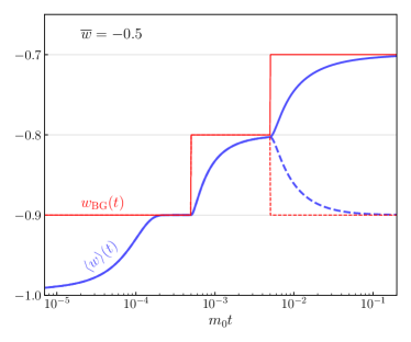
Figure 11: Tracking behavior for the stasis state resulting from a tower of scalar fields in the presence of a variable background. Even when a stasis is achieved for the tower of scalar fields, any subsequent change in $w_{\rm BG}$ destabilizes the existing stasis and produces a new stasis for which $\langle w\rangle$ continues to match $w_{\rm BG}$. This behavior persists as long as the new value of $w_{\rm BG}$ continues to be smaller than $\overline{w}$. In this figure, two sets of changes for $w_{\rm BG}$ are shown: in one case (shown in solid red), the background has a value of $w_{\rm BG}$ which starts at $-0.9$ and subsequently jumps to $-0.8$ and then $-0.7$, while in the other case (dashed red), the background behaves identically except that the final jump is back down to $w_{\rm BG}=-0.9$ rather than to $-0.7$. In both cases, the values of $\langle w\rangle$ for our scalar-field tower (shown in blue) attempt to track the behavior of the background, achieving short-lived stases with $\langle w\rangle=w_{\rm BG}$ within each interval before becoming destabilized again. The blue curves in this figure are calculated assuming an initial background abundance $\Omega_{\rm BG}^{(0)}=0.98$, but the same qualitative results would emerge for any value of $\Omega_{\rm BG}^{(0)}$ and any sequence of $w_{\rm BG}$-values which are all smaller than $\overline{w}$.

Let us now consider what happens when the equation-of-state parameter $w_{\rm BG}$ is time-dependent. We have already seen that when $w_{\rm BG}$ is a constant, and when this constant is smaller than $\overline{w}$, the dynamics of our $\phi_{\ell}$ tower adjusts in order to realize a stasis with $\overline{w}^{\prime}=w_{\rm BG}$. It is therefore important to understand how our system responds when $w_{\rm BG}$ itself is changing.

In general, the time variation of $w_{\rm BG}(t)$ can be modeled as a sequence of discrete jumps:

$$w_{\rm BG}(t)~{}=~{}w_{\rm BG}^{(0)}+\sum_{\{i\}}\Delta^{(i)}\,\Theta(t-t_{i})~{}$$ (78)

where $\{i\}$ labels an arbitrary collection of times $t_{i}$ at which $w_{\rm BG}$ suddenly changes by an amount $\Delta^{(i)}$. In the infinitesimal limit of such jumps, one can obtain a continuous time dependence.

We show two examples of such jumps in Fig. 11. In each of these examples, $w_{\rm BG}$ experiences two instantaneous jumps with $\left|\Delta^{(i)}\right|=0.1$. In the case represented by the solid red curve, $w_{\rm BG}$ increases twice. By contrast, in the case represented by the dashed red curve, $w_{\rm BG}$ increases once and then drops back to its original value.

In Fig. 11, we also indicate the response of a system with $\overline{w}=-0.5$ to these sequences of jumps. For each sequence of jumps, we see that the equation-of-state parameter $\left\langle w\right\rangle$ for our dynamical-scalar system (represented by the corresponding blue curve) always attempts to match these discrete changes in $w_{\rm BG}$, and even occasionally has enough time to achieve a short-lived stasis with $\langle w\rangle\to\overline{w}^{\prime}=w_{\rm BG}$ until $w_{\rm BG}$ changes again. We also observe from Fig. 11 that this tracking is not instantaneous. In particular, although any stasis that has already been achieved is immediately destabilized when $w_{\rm BG}$ changes, it takes a non-zero amount of time for the system to realize the new stasis for which the new value of $\left\langle w\right\rangle$ matches the new value of $w_{\rm BG}$. It is nevertheless intriguing to see that the tower is capable of adjusting its internal dynamics spontaneously in order to follow the change in the external background.

Such tracking behavior is not unexpected. After all, our stasis solution is a global attractor. As a result, any change in $w_{\rm BG}$ simply amounts to moving the location of the attractor within the phase space. Of course, the trajectory lines towards the original attractor are different from the trajectory lines towards the new attractor. However, any point on an original trajectory line is also a point on a new trajectory line. Thus, at the moment when $w_{\rm BG}$ changes, our system simply begins to evolve along the new trajectory line rather the previous one. For this reason, even if the background equation-of-state parameter varies continuously, the tower will always evolve in such a manner as to track $w_{\rm BG}$. Of course, a perfect slow-roll/oscillatory-component stasis with $\langle w\rangle=w_{\rm BG}$ can only be expected once $w_{\rm BG}$ stabilizes to a constant.

V Towards a stasis-induced inflation

The results derived in Sects. III and IV suggest that stasis could be the foundation of a deep connection between cosmology and particle physics. Such a connection could then open the door to many new ways of thinking about the physics of the early universe. Along these lines, one of the most exciting ideas that emerges from this work is the possibility that the stasis phenomenon we have discussed in this paper might serve as the foundation for a new approach to cosmological inflation. In this section, we shall therefore outline some speculative thoughts concerning this possibility.

It is not hard to see that the stasis phenomenon could provide the underpinning of a possible new way of realizing cosmic inflation. After all, as we have demonstrated, our system of rolling scalars can give rise to a stasis epoch during which the abundances of matter and vacuum energy remain fixed and in which the universe expands with an equation of state within the range $-1<\overline{w}<0$. Thus, if our initial conditions are such that $\overline{w}<-1/3$ (so that the universe experiences an accelerated expansion with $\ddot{a}>0$ during stasis), and if this stasis is maintained for a sufficient number of $e$-folds, we will have produced an epoch of accelerated expansion which could potentially explain the extraordinary flatness and homogeneity of our universe. This could then serve as the basis of a new model of cosmic inflation.

We shall refer to this intriguing possibility as a stasis-induced inflation, or simply “Stasis Inflation”. As it turns out, Stasis Inflation has a number of interesting features which merit further exploration.

First of all, Stasis Inflation does not require a complicated scalar potential. Moreover, it does not rely on non-minimal coupling structures between the scalar sector and gravity, unlike many of the inflationary scenarios that have been proposed in order to accommodate the most recent CMB measurements Ade et al. (2021); Akrami et al. (2020a). Indeed, the dynamics which gives rise to the accelerated expansion in Stasis Inflation does not follow primarily from the shape of the potential but rather from the structure of the underlying particle physics. Moreover, in cases wherein the $\phi_{\ell}$ are the KK modes of a higher-dimensional scalar field, the mass spectrum of such states is primarily a reflection of the compactification geometry.

Second, we observe that any equation-of-state parameter $\overline{w}<-1/3$ for the stasis sector can be realized within our Stasis Inflation framework. Thus, it is relatively straightforward to achieve an epoch of accelerated cosmological expansion within this scenario, and we are not restricted to having $\overline{w}\approx-1$.

Third, within the most natural realizations of Stasis Inflation the number of $e$-folds of inflation is no longer a free parameter but is directly related to the hierarchies between particle-physics scales. For example, for scenarios in which the $\phi_{\ell}$ tower consists of the KK excitations of a higher-dimensional scalar field, the number of such states will generically scale as $N\sim(RM_{\rm UV})^{n}$ where $R$ schematically denotes a compactification radius, where $M_{\rm UV}$ denotes a UV cutoff such as the string scale or the Planck scale, and where $n$ is the number of compactified dimensions. We thus see that the number of states in the tower — and thus the duration of the stasis epoch or equivalently the number of $e$-folds of cosmic inflation produced — is directly connected to the hierarchy between $R^{-1}$ and $M_{\rm UV}$. Taking $R^{-1}\sim{\cal O}({\rm TeV})$ and $M_{\rm UV}\sim{\cal O}(M_{\rm Planck})$ — as is typical in theories involving large extra dimensions — we see that this hierarchy can be significant. Such models would then lead us to conclude that the universe is large simply because the Planck/TeV hierarchy is big! This thereby provides a novel connection between two large numbers in physics.

Fourth, the Stasis Inflation scenario has a natural graceful exit. Indeed, the stasis epoch ends when the transitions from (overdamped) vacuum energy to (underdamped) matter have reached the bottom of the $\phi_{\ell}$ tower. As we have seen, this sort of exit is a general feature of all stasis epochs, and as such a graceful exit from accelerated expansion is already an inherent part of the Stasis Inflation scenario.

But finally — and perhaps most importantly — Stasis Inflation behaves differently than ordinary inflation in terms of its effects on the abundances of vacuum energy, matter, radiation, and potentially even other energy components in the universe. Normally, during traditional inflationary epochs, the universe rapidly becomes dominated by vacuum energy, and all other energy components that might have existed at the start of inflation will inflate away, with abundances that fall to zero. This is ultimately why an epoch of reheating is generally required after traditional inflation. However, with Stasis Inflation, the situation is different: a non-zero matter abundance can be carried along throughout the inflationary epoch without exhibiting any reduction, even though the universe is undergoing an accelerated expansion with $\overline{w}<-1/3$. This is ultimately because vacuum energy and matter together play a crucial role in sustaining the inflationary stasis that drives the cosmological inflation. Moreover, if we further allow our scalar fields to decay to radiation, as discussed in Ref. Dienes et al. (2024), we can even achieve an inflationary triple stasis involving not only vacuum energy and matter but also radiation. Thus the abundances of vacuum energy, matter, and radiation can all be sustained across the inflationary epoch. This has the potential to significantly change the conditions needed for any subsequent reheating.

In this section we have provided only a rough qualitative sketch of a possible Stasis Inflation scenario. Much more work is needed in order to determine whether such a scenario is phenomenologically viable. For example, Stasis Inflation must be shown to generate the correct power spectrum for scalar perturbations while satisfying current bounds on tensor perturbations Ade et al. (2021); Akrami et al. (2020a). Similarly, one must examine the generation of non-Gaussianities and isocurvature perturbations within such scenarios and determine whether the results are consistent with current observational constraints Akrami et al. (2020b, a). Stasis Inflation nevertheless remains an interesting possibility worthy of further exploration.

VI Discussion and conclusions

Towers comprising large numbers of scalar fields are a common feature of many BSM scenarios, including theories with extra spacetime dimensions and string theory. Moreover, the homogeneous zero-mode field value associated with each of these fields transitions dynamically from an overdamped phase exhibitng slow-roll behavior to an underdamped phase exhibiting rapid oscillations. In this paper, we have examined the conditions under which the full dynamics of such fields across the tower can give rise to an epoch of cosmic stasis between the collective slow-roll and oscillatory abundances associated with these two phases.

In the simplest case one might consider — that in which no additional cosmological energy components are present and in which the masses and initial abundances of these scalars across the tower follow the scaling relation in Eq. (24) — we found that a cosmological stasis can develop during which these two collective abundances $\Omega_{\rm SR}$ and $\Omega_{\rm osc}$ each remain constant despite cosmic expansion across many $e$-folds. Indeed, a stasis of this sort arises generically in any such system, provided that our mass and abundance scaling exponents $\delta$ and $\alpha$ satisfy $\alpha+1/\delta=2$ and provided that the density of states per unit mass within the tower is sufficiently large that the mass spectrum may reliably be approximated as a continuum. Moreover, we also demonstrated that in such circumstances, the stasis state is actually a cosmological attractor. Depending on initial conditions, the ultimate stasis abundances ${\overline{\Omega}}_{\rm SR}$ and ${\overline{\Omega}}_{\rm osc}$ can take any value within the ranges $0<{\overline{\Omega}}_{\rm SR}<1$ and $0<{\overline{\Omega}}_{\rm osc}<1$, with ${\overline{\Omega}}_{\rm SR}+{\overline{\Omega}}_{\rm osc}=1$. As a result, the effective equation-of-state parameter for the universe as a whole during stasis can take any value within the range $-1<{\overline{w}}<0$.

We also considered how this picture changes in the presence of an additional background energy component beyond the scalar tower — a component that we take to be a perfect fluid with a constant equation-of-state parameter $w_{\rm BG}$ and arbitrary initial abundance $\Omega_{\rm BG}^{(0)}$. We found that a stasis always emerges in this case as well. However, we found that the properties of this stasis depend on the relative sizes between $w_{\rm BG}$ and $\overline{w}$, where $\overline{w}$ is the effective equation-of-state parameter of the stasis that would have emerged in the absence of this additional cosmological energy component. When $w_{\rm BG}>{\overline{w}}$, we found that the background energy density $\rho_{\rm BG}$ decreases more rapidly with cosmic expansion than does the energy density of the tower. Thus the properties of the resulting asymptotic stasis are unaffected by the presence of the background, and our tower gives rise to the same stasis as before. By contrast, in cases in which $w_{\rm BG}<{\overline{w}}$, we found that the tower gives rise to an entirely new stasis — a tracking stasis — in which the new equation-of-state parameter ${\overline{w}}^{\prime}$ evolves toward the value $w_{\rm BG}$. Indeed, this is true regardless of the initial background abundance $\Omega_{\rm BG}^{(0)}$.

Finally, we speculated that these ideas might form the basis of a new approach towards understanding cosmic inflation. Indeed, a stasis epoch of this sort with $\overline{w}<-1/3$ exhibits accelerated expansion, and could potentially solve the flatness and hierarchy problems. Moreover, as we discussed, this sort of “Stasis Inflation” has a number of intriguing and potentially beneficial properties not shared by traditional models of inflation. Of course, a more detailed examination of this idea is necessary before any conclusions concerning its viability can be drawn.

A few comments are in order. First, since the particular form of stasis that we have examined in this paper arises from the collective dynamics of a large number of scalar fields whose masses and abundances exhibit particular scaling behaviors, it is important to consider how these scaling behaviors might arise in actual models of particle physics. Fortunately, the mass spectrum that we considered in this paper — a spectrum characterized by a scaling exponent $\delta$, a mass-splitting parameter $\Delta m$, and a ground-state mass shift $m_{0}$ — is a fairly generic one in many extensions of the Standard Model, including those extensions involving extra compact spacetime dimensions. Moreover, the spectrum of initial abundances that we considered is one in which the $\Omega_{\ell}^{(0)}$ scale with $m_{\ell}$ according to a power law. As we have discussed, this too is a fairly generic result emerging from many different types of production mechanisms.

Given the requirements of stasis, we found that the spectrum of initial field displacements $\phi_{\ell}^{(0)}$ in our model must scale as $\phi_{\ell}^{(0)}\sim\ell^{-1/2}$, assuming all such fields start from rest. While such a spectrum of initial displacements is in principle achievable in scenarios in which the $\phi_{\ell}$ are the KK excitations of a higher-dimensional scalar field, it would be interesting to explore how such a spectrum might emerge within the framework of a more fully developed model of higher-dimensional physics. Of course, explicit model constructions exist in the literature Dienes and Thomas (2012a, b, c) wherein the initial abundances $\Omega_{\ell}^{(0)}$ and masses $m_{\ell}$ obey the same scaling relations across a tower of axion-like particles as we have assumed here, with scaling exponents $\alpha$ and $\delta$ respectively. Those models were developed in order to address the dark-matter problem, and there is even a partial overlap in the $(\alpha,\delta)$ parameter space between what is required for those models and what we require for stasis. However, it still remains to construct explicit particle-physics models within that overlap region.

Second, while we have focused in this paper on the case in which the potentials for the $\phi_{\ell}$ are quadratic, there are also other forms for the potential which are of interest from a model-building perspective. One of these is the form

$$V(\phi_{\ell})~{}=~{}\sum_{i}\,\Lambda_{i}\,\exp\left(\sum_{\ell}\alpha_{i\ell}\,\phi_{\ell}\right)~{},$$ (79)

where the $\Lambda_{i}$ and $\alpha_{i\ell}$ are model-dependent constants. Potentials of this form arise in the low-energy limit of string compactifications and are of significant interest because they can give rise to so-called scaling cosmologies Calderón-Infante et al. (2023); Shiu et al. (2023a, b) in which the scale factor $a(t)$ evolves with time $t$ according to a power law. While such potentials lack stable minima, it is nevertheless conceivable that they could also give rise to a stasis epoch. Indeed, in such stasis scenarios, the equation-of-state parameter $w_{\ell}$ for each $\phi_{\ell}$ field is approximately $w_{\ell}(t)\approx-1$ at early times. However, since there is no potential minimum, each field continues rolling, and the energy density of the field eventually becomes dominated by kinetic energy. As a result, $w_{\ell}(t)\approx 1$ at late times. It would be interesting to investigate the extent to which this dynamical evolution from smaller to larger values of $w_{\ell}(t)$ can compensate for the effect of cosmological expansion, and whether this effect can therefore also give rise to stasis. We leave this possibility for future work.

Third and finally, we emphasize again that the ideas in this paper could serve as the foundation of a deep connection between cosmology and particle physics and thereby open the door to many exciting phenomenological implications of cosmic stasis. For example, as discussed in Sect. V, a stasis epoch with ${\overline{w}}<-1/3$ persisting for $\mathcal{N}_{s}\gtrsim 60$ $e$-folds of cosmic expansion can in principle constitute a solution to the flatness and horizon problems. If indeed viable models of Stasis Inflation could be developed along these lines, such models would almost certainly give rise to distinctive power spectra of primordial scalar and tensor perturbations. This opens the possibility that evidence for Stasis Inflation could potentially be extracted from observations of the CMB and/or the stochastic gravitational-wave background. Another possibility is that a stasis involving dynamical scalars could occur much later in the cosmological timeline. In particular, it would be interesting to consider the possibility that the slowly rolling $\phi_{\ell}$ could collectively constitute the dark energy which drives the accelerated expansion that we observe at the present time, while the oscillatory $\phi_{\ell}$ could collectively constitute the dark matter. Of course, the presence of large numbers of extremely light axion-like scalars presents a number of model-building challenges, including those imposed by constraints on supernova energy loss Raffelt and Seckel (1988); Olive and Pospelov (2008), Eötvös-type experiments Chen et al. (2016); Tan et al. (2020), searches for frequency variation in atomic clocks Arvanitaki et al. (2015), black-hole superradiance considerations Arvanitaki and Dubovsky (2011); Brito et al. (2015); Cardoso et al. (2018); Stott and Marsh (2018); Stott (2020); Mehta et al. (2020), and data from pulsar-timing arrays Blas et al. (2017); Kaplan et al. (2022). That said, if one were to construct a phenomenologically viable model of dark energy along these lines, it would go a long way toward addressing the cosmic coincidence problem. This topic is therefore worthy of further exploration.