Conformal Prediction for Class-wise Coverage
via Augmented Label Rank Calibration

Abstract

Conformal prediction (CP) is an emerging uncertainty quantification framework that allows us to construct a prediction set to cover the true label with a pre-specified marginal or conditional probability. Although the valid coverage guarantee has been extensively studied for classification problems, CP often produces large prediction sets which may not be practically useful. This issue is exacerbated for the setting of class-conditional coverage on imbalanced classification tasks. This paper proposes the Rank Calibrated Class-conditional CP (RC3P) algorithm to reduce the prediction set sizes to achieve class-conditional coverage, where the valid coverage holds for each class. In contrast to the standard class-conditional CP (CCP) method that uniformly thresholds the class-wise conformity score for each class, the augmented label rank calibration step allows RC3P to selectively iterate this class-wise thresholding subroutine only for a subset of classes whose class-wise top-$k$ error is small. We prove that agnostic to the classifier and data distribution, RC3P achieves class-wise coverage. We also show that RC3P reduces the size of prediction sets compared to the CCP method. Comprehensive experiments on multiple real-world datasets demonstrate that RC3P achieves class-wise coverage and $26.25\%$ $\downarrow$ reduction in prediction set sizes on average.

1 Introduction

Safe deployment of machine learning (ML) models in high stakes applications such as medical diagnosis requires theoretically-sound uncertainty estimates. Conformal prediction (CP) [11] is an emerging uncertainty quantification framework that constructs a prediction set of candidate output values such that the true output is present with a pre-specified level (e.g., $\geq 90\%$) of the marginal or conditional probability [39, 40]. A promising property of CP is the model-agnostic and distribution-free coverage validity under certain notions [42]. For example, marginal coverage is the commonly studied validity notion [9, 20, 39], while conditional coverage is a stronger notion. There is a general taxonomy to group data (i.e., input-output pairs) into categories and to study the valid coverage for each group (i.e., the group-wise validity) [44, 11]. This paper focuses on the specific notion of class-conditional coverage that guarantees coverage for each class individually, which is important for imbalanced classification tasks (e.g., medical applications) [41, 47, 48].

In addition to the coverage validity, predictive efficiency is another important criterion for CP [42, 46], which refers to the size of the prediction sets. Both coverage validity and predictive efficiency are used together to measure the performance of CP methods [20, 38, 9, 33, 1, 43]. Since the two measures are competing [20], our goal is to guarantee the coverage validity with high predictive efficiency, i.e., small prediction sets [42, 9, 43]. Some studies improved the predictive efficiency under the marginal coverage setting using new conformity score function [20, 35] and new calibration procedures [40, 43, 19, 36]. However, it is not known if these methods will benefit the predictive efficiency for the class-conditional coverage setting. A very recent work [33] proposed the cluster CP method to approximate class-conditional coverage. It empirically improves predictive efficiency over the baseline class-wise CP method (i.e., each class is one cluster) [30], but the approximation guarantee for class-wise coverage is model-dependent (i.e., requires certain assumptions on the model). The main question of this paper is: how can we develop a model-agnostic CP algorithm that guarantees the class-wise coverage with improved predictive efficiency (i.e., small prediction sets)?

To answer this question, we propose a novel approach referred to as Rank Calibrated Class-conditional CP (RC3P) that guarantees the class-wise coverage with small expected prediction sets. The class-conditional coverage validity of RC3P is agnostic to the data distribution and the underlying ML model, while the improved predictive efficiency depends on very mild conditions of the given trained classifier. The main ingredient behind the RC3P method is the label rank calibration strategy augmented with the standard conformal score calibration from the class-wise CP (CCP) [30, 21].

The CCP method finds the class-wise quantiles of non-conformity scores on calibration data. To produce the prediction set for a new test input $X_{\text{test}}$, it pairs $X_{\text{test}}$ with each candidate class label $y$ and includes the label $y$ if the non-conformity score of the pair $(X_{\text{test}},y)$ is less than or equal to the corresponding class-wise quantile associated with $y$. Thus, CCP constructs the prediction set by uniformly iterating over all candidate labels. In contrast, the label rank calibration allows RC3P to selectively iterate this class-wise thresholding subroutine only if the label $y$ is ranked by the classifier $f(X_{\text{test}})$ (e.g., $f(\cdot)$ denotes the softmax prediction) in the top $k_{y}$ candidates, where the value of $k_{y}$ is calibrated for each label $y$ individually according to the class-wise top-$k_{y}$ error. In other words, given $X_{\text{test}}$, RC3P enables standard class-wise conformal thresholding for the sufficiently certain class labels only (as opposed to all labels). Our theory shows that the class-wise coverage provided by RC3P is agnostic to the data distribution and the underlying ML model. Moreover, under a very mild condition, RC3P guarantees improved predictive efficiency over the baseline CCP method.

Contributions. The main contributions of this paper are:

• We design a novel algorithm RC3P that augments the label rank calibration strategy to the standard conformal score calibration step. To produce prediction sets for new inputs, it selectively performs class-wise conformal thresholding only on a subset of classes based on their corresponding calibrated label ranks.

• We develop theoretical analysis to show that RC3P guarantees class-wise coverage, which is agnostic to the data distribution and trained classifier. Moreover, it provably produces smaller average prediction sets over the baseline CCP method [30].

• We perform extensive experiments on multiple imbalanced classification datasets and show that RC3P achieves the class-wise coverage with significantly improved predictive efficiency over the existing class-conditional CP baselines ($26.25\%$ reduction in the prediction size on average on all four datasets or $35\%$ reduction excluding CIFAR-10).

2 Related Work

Precise uncertainty quantification of machine learning based predictions is necessary in high-stakes decision-making applications. It is especially challenging for imbalanced classification tasks. Although many imbalanced classification learning algorithms [5, 29] are proposed, e.g., re-sampling [22, 24, 25, 23, 26] and re-weighting [27, 28], they do not provide uncertainty quantification with rigorous guarantees over predictions for each class.

Conformal prediction [14, 11] is a model-agnostic and distribution-free framework for uncertainty quantification by producing prediction sets that cover the true output with a pre-specified probability, which means CP could provide valid coverage guarantee with any underlying model and data distribution [61, 62, 63]. Many CP algorithms are proposed for regression [58, 34, 16, 60], classification [38, 20, 52, 53], structured prediction [49, 50, 51, 57], online learning [55, 59], and covariate shift [56, 17, 54] settings. Coverage validity and predictive efficiency are two common and competing desiderata for CP methods [20]. Thus, small prediction sets are favorable whenever the coverage validity is guaranteed [42, 9, 43], e.g., human and machine learning collaborative systems [41, 47, 48]. Recent work improved the predictive efficiency for marginal coverage by designing new conformity score [20, 35] and calibration procedures [40, 43, 19, 36]. These methods can be combined with class-conditional CP methods including RC3P as we demonstrate in our experiments, but the effect on predictive efficiency is not clear.

In general, the methods designed for a specific coverage validity notion are not necessarily compatible with another notion of coverage, such as object-conditional coverage [30], class-conditional coverage [30], local coverage [45] which are introduced and studied in the prior CP literature [44, 11, 42, 33, 37]. The standard class-conditional CP method in [30, 18] guarantees the class-wise coverage, but does not particularly aim to reduce the size of prediction sets. The cluster CP method [33] which performs CP over clusters of labels achieves a cluster-conditional coverage that approximates the class-conditional guarantee, but requires some assumptions on the underlying clustering model.

Our goal is to develop a provable class-conditional CP algorithm with small prediction sets to guarantee the class-wise coverage that is agnostic to the underlying model.

3 Notations, Background, and Problem Setup

Notations. Suppose $(X,Y)$ is a data sample where $X\in\mathcal{X}$ is an input from the input space $\mathcal{X}$, and $Y\in\mathcal{Y}=\{1,2,\cdots,K\}$ is the ground-truth label with $K$ candidate classes. Assume $(X,Y)$ is randomly drawn from an underlying distribution $\mathcal{P}$ defined on $\mathcal{X}\times\mathcal{Y}$, where we denote $p_{y}=\mathbb{P}_{XY}[Y=y]$. Let $f:\mathcal{X}\rightarrow\Delta_{+}^{K}$ denote a soft classifier (e.g., a soft-max classifier) that produces prediction scores for all candidate classes on any given input $X$, where $\Delta_{+}^{K}$ denote the $K$-dimensional probability simplex and $f(X)_{y}$ denotes the predicted confidence for class $y$. We define the class-wise top-$k$ error for class $y$ from the trained classifier $f$ as $\epsilon_{y}^{k}=\mathbb{P}\{r_{f}(X,Y)>k|Y=y\}$, where $r_{f}(X,Y)=\sum_{l=1}^{K}\mathbbm{1}[f(X)_{l}\geq f(X)_{Y}]$ returns the rank of $Y$ predicted by $f(X)$ in a descending order, and $\mathbbm{1}[\cdot]$ is an indicator function. We are provided with a training set $\mathcal{D}_{\text{tr}}$ for training the classifier $f$, and a calibration set $\mathcal{D}_{\text{cal}}=\{(X_{i},Y_{i})\}_{i=1}^{n}$ for CP. Let $\mathcal{I}_{y}=\{i:Y_{i}=y,\text{ for all }(X_{i},Y_{i})\in\mathcal{D}_{\text{cal}}\}$ and $n_{y}=|\mathcal{I}_{y}|$ denote the number of calibration examples for class $y$.

Table 1: Key notations used in this paper.

Notation	Meaning
$X\in\mathcal{X}$	Input example
$Y\in\mathcal{Y}$	The ground-truth label
$f$	The soft classifier
$\Delta_{+}^{K}$	The $K$-dimensional probability simplex
$f(X)_{y}$	The predicted confidence on class $y$
$\epsilon_{y}^{k}$	The class-wise top-$k$ error for class $y$ from $f$
$r_{f}(X,Y)$	The rank of $Y$ predicted by $f(X)$
$\mathcal{D}_{\text{tr}}$	Training data
$\mathcal{D}_{\text{cal}}$	Calibration data
$\mathcal{D}_{\text{test}}$	Test data
$n_{y}$	The number of calibration examples for class $y$
$V(X,Y)$	Non-conformity scoring function
$\mathcal{C}_{1-\alpha}(X_{\text{test}})$	Prediction set for input $X_{\text{test}}$
$\alpha$	Target mis-coverage rate
$\widehat{\alpha}_{y}$	Nominal mis-coverage rate for class $y$

Problem Setup of CP. Let $V:\mathcal{X}\times\mathcal{Y}\rightarrow\mathbb{R}$ denote a non-conformity scoring function to measure how different a new example is from old ones [11]. It is employed to compare a given testing sample $(X_{\text{test}},Y_{\text{test}})$ with a set of calibration data $\mathcal{D}_{\text{cal}}$: if the non-conformity score is large, then $(X_{\text{test}},Y_{\text{test}})$ conforms less to calibration samples. Prior work has considered the design of good non-conformity scoring functions, e.g., [21, 15, 9]. In this paper, we focus on the scoring functions of Adaptive Prediction Sets (APS) proposed in [9] and Regularized APS (RAPS) proposed in [20] for classification based on the ordered probabilities of $f$ and true label rank $r_{f}(X,Y)$. For the simplicity of notation, we denote the non-conformity score of the $i$-th calibration example as $V_{i}=V(X_{i},Y_{i})$.

Given a input $X$, we sort the predicted probability for all classes {$1,\cdots,K$} of the classifier $f$ such that $1\geq f(X)_{(1)}\geq\cdots\geq f(X)_{(K)}\geq 0$ are ordered statistics, where $f(X)_{(k)}$ denotes the $k$-th largest prediction. The APS [9] score for a sample $(X,Y)$ is computed as follows:

$$V(X,Y)=\sum_{l=1}^{r_{f}(X,Y)-1}f(X)_{(l)}+U\cdot f(X)_{(r_{f}(X,Y))},$$

where $U\in[0,1]$ is a uniform random variable to break ties. We also consider its regularized variant RAPS [20], which additionally includes a rank-based regularization $\lambda(r_{f}(X,Y)-k_{reg})^{+}$ to the above equation, where $(\cdot)^{+}=\text{max}\{0,\cdot\}$ denotes the hinge loss, $\lambda$ and $k_{reg}$ are two hyper-parameters.

For a target coverage $1-\alpha$, we find the corresponding empirical quantile on calibration data $\mathcal{D}_{\text{cal}}$ defined as

$$\widehat{Q}_{1-\alpha}=\text{min}\Big{\{}t:\sum_{i=1}^{n}\frac{1}{n}\cdot\mathbbm{1}[V_{i}\leq t]\geq 1-\alpha\Big{\}},$$

which can be determined by finding the $\lceil(1-\alpha)(1+n)\rceil$-th smallest value of $\{V_{i}\}_{i=1}^{n}$. The prediction set of a testing input $X_{\text{test}}$ can be constructed by thresholding with $\widehat{Q}_{1-\alpha}$:

$$\widehat{\mathcal{C}}_{1-\alpha}(X_{\text{test}})=\{y\in\mathcal{Y}:V(X_{\text{test}},y)\leq\widehat{Q}_{1-\alpha}\}.$$

Therefore, $\widehat{\mathcal{C}}_{1-\alpha}$ gives a marginal coverage guarantee [9, 20]: $\mathbb{P}_{(X,Y)\sim\mathcal{P}}\{Y\in\widehat{\mathcal{C}}_{1-\alpha}(X)\}\geq 1-\alpha.$ To achieve the class-conditional coverage, standard CCP [30] uniformly iterates the class-wise thresholding subroutine with the class-wise quantiles $\{\widehat{Q}_{1-\alpha}^{\text{class}}(y)\}_{y\in\mathcal{Y}}$:

$$~{}~{}~{}\widehat{\mathcal{C}}^{\text{CCP}}_{1-\alpha}(X_{\text{test}})=\{y\in\mathcal{Y}:V(X_{\text{test}},y)\leq\widehat{Q}_{1-\alpha}^{\text{class}}(y)\},$$ (1)

$$\qquad\qquad\text{where }\widehat{Q}_{1-\alpha}^{\text{class}}(y)=\text{min}\Big{\{}t:\sum_{i\in\mathcal{I}_{y}}\frac{1}{n_{y}}\cdot\mathbbm{1}[V_{i}\leq t]\geq 1-\alpha\Big{\}}.$$

Specifically, CCP pairs $X_{\text{test}}$ with each candidate class label $y$, and includes $y$ in the prediction set $\widehat{\mathcal{C}}^{\text{CCP}}_{1-\alpha}(X_{\text{test}})$ if $V(X_{\text{test}},y)\leq\widehat{Q}_{1-\alpha}^{\text{class}}(y)$ holds. After going through all candidate class labels $y\in\mathcal{Y}$, it achieves the class-wise coverage for any $y\in\mathcal{Y}$ [30, 21]:

$$\mathbb{P}_{(X,Y)\sim\mathcal{P}}\{Y\in\widehat{\mathcal{C}}^{\text{CCP}}_{1-\alpha}(X)|Y=y\}\geq 1-\alpha.$$ (2)

CCP produces large prediction sets which are not useful in practice. Therefore, our goal is to develop a provable CP method that provides class-conditional coverage and constructs smaller prediction sets than those from CCP. We summarize all the notations in Table 1.

4 Rank Calibrated Class-Conditional CP

We first explain the proposed Rank Calibrated Class-conditional Conformal Prediction (RC3P) algorithm and present its model-agnostic coverage guarantee. Next, we provide the theoretical analysis for the provable improvement of predictive efficiency of RC3P over the CCP method.

4.1 Algorithm and Model-Agnostic Coverage Analysis

We start with the motivating discussion about the potential drawback of the standard CCP method in terms of predictive efficiency. Equation (1) shows that, for a given test input $X_{\text{test}}$, CCP likely contains some uncertain labels due to the uniform iteration over each class label $y\in\mathcal{Y}$ to check if $y$ should be included into the prediction set or not. For example, given a class label $y$ and two test samples $X_{1},X_{2}$, suppose their APS scores are $V(X_{1},y)=0.9,V(X_{2},y)=0.8$, with ranks $r_{f}(X_{1},y)=1,r_{f}(X_{2},y)=5$. Furthermore, if $\widehat{Q}_{1-\alpha}^{\text{class}}(y)=0.85$, then by (1) for CCP, we know that $y\notin\widehat{\mathcal{C}}^{\text{CCP}}_{1-\alpha}(X_{1})$ and $y\in\widehat{\mathcal{C}}^{\text{CCP}}_{1-\alpha}(X_{2})$, even though $f(X_{1})$ ranks $y$ at the #1 class label for $X_{1}$ with a very high confidence $f(X_{1})_{y}=0.9$ and CCP can still achieve the valid class-conditional coverage. We argue that, the principle of CCP that scans all $y\in\mathcal{Y}$ uniformly can easily result in large prediction sets, which is detrimental to human-ML collaboration [3, 2].

Consequently, to improve the predictive efficiency of CCP (i.e., reduce prediction set sizes), it is reasonable to include label rank information in the calibration procedure to adjust the distribution of non-conformity scores for predictive efficiency. As mentioned in the previous sections, better scoring functions have been proposed to improve the predictive efficiency for marginal coverage, e.g., RAPS. However, directly applying RAPS for class-wise coverage presents challenges: 1) tuning its hyper-parameters for each class requires extra computational overhead, and 2) fixing its hyper-parameters for all classes overlooks the difference between distributions of different classes. Moreover, for the approximate class-conditional coverage achieved by cluster CP [33], it still requires some assumptions on the underlying model (i.e., it is not fully model-agnostic).

Algorithm 1 RC3P  Method for Class-Conditional CP

1:  Input: Mis-coverage rate $\alpha\in(0,1)$., top-$k$ errors $\epsilon_{y}^{k}$ for all classes and ranks $y,k\in\{1,\cdots,K\}$

2:  Randomly split data into train $\mathcal{D}_{\text{tr}}$ and calibration $\mathcal{D}_{\text{cal}}$ and train the classifier $f$ on $\mathcal{D}_{\text{tr}}$

3:  for  $y\in\{1,\cdots,K\}$  do

4:     Compute $\{V_{i}\}_{i=1}^{n_{y}}$ for all $(X_{i},Y_{i})\in\mathcal{D}_{\text{cal}}$ such that $Y_{i}=y$

5:     Configure calibrated label rank $\widehat{k}(y)$ and nominal error $\widehat{\alpha}_{y}$:

6:      Option I (model-agnostic coverage):    $\widehat{k}(y)\in\{k:\epsilon_{y}^{k}<\alpha\},~{}~{}0\leq\widehat{\alpha}_{y}\leq\alpha-\epsilon_{y}^{\widehat{k}(y)}$, as per Eq (4)

7:      Option II (model-agnostic coverage + improved predictive efficiency):    $\widehat{k}(y)=\text{min}\{k:\epsilon_{y}^{k}<\alpha\},~{}~{}\widehat{\alpha}_{y}=\alpha-\epsilon_{y}^{\widehat{k}(y)}$, as per Eq (7)

8:     $\widehat{Q}^{\text{class}}_{1-\widehat{\alpha}_{y}}(y)\leftarrow\lceil(1-\widehat{\alpha}_{y})(1+n_{y})\rceil$-th smallest value in $\{V_{i}\}_{i=1}^{n_{y}}$ according to Eq (1)

9:  end for

10:  Construct $\widehat{\mathcal{C}}^{\text{RC3P}}_{1-\alpha}(X_{\text{test}})$ with $\widehat{Q}^{\text{class}}_{1-\widehat{\alpha}_{y}}(y)$ and $\widehat{k}(y)$ for a test input $X_{\text{test}}$ using Eq (3)

Therefore, the key idea of our proposed RC3P algorithm (outlined in Algorithm 1) is to refine the class-wise calibration procedure using a label rank calibration strategy augmented to the standard conformal score calibration, to enable adaptivity to various classes. Specifically, in contrast to CCP, RC3P selectively activates the class-wise thresholding subroutine in (1) according to their class-wise top-$k$ error $\epsilon_{y}^{k}$ for class $y$. RC3P produces the prediction set for a given test input $X_{\text{test}}$ with two calibration schemes (one for conformal score and another for label rank) as shown below:

$$\widehat{\mathcal{C}}^{\text{RC3P}}_{1-\alpha}(X_{\text{test}})=\big{\{}y\in\mathcal{Y}:\underbrace{V(X_{\text{test}},y)\leq\widehat{Q}^{\text{class}}_{1-\widehat{\alpha}_{y}}(y)}_{\text{conformal score calibration }},~{}\underbrace{r_{f}(X_{\text{test}},y)\leq\widehat{k}(y)}_{\text{ label rank calibration }}\big{\}},$$ (3)

where $\widehat{Q}_{1-\widehat{\alpha}_{y}}^{\text{class}}(y)$ and $\widehat{k}(y)$ are score and label rank threshold for class $y$, respectively. In particular, $\widehat{k}(y)$ controls the class-wise uncertainty adaptive to each class $y$ based on the top-$k$ error $\epsilon_{y}^{\widehat{k}(y)}$ of the classifier. By determining $\widehat{k}(y)$, the top $k$ predicted class labels of $f(X_{\text{test}})$ will more likely cover the true label $Y_{\text{test}}$, making the augmented label rank calibration filter out the class labels $y$ that have a high rank (larger $r_{f}(X,y)$). As a result, given all test input and label pairs $\{(X_{\text{test}},y)\}_{y\in\mathcal{Y}}$, RC3P performs score thresholding using class-wise quantiles only on a subset of reliable test pairs.

Determining $\widehat{k}(y)$ and $\widehat{\alpha}_{y}$ for model-agnostic valid coverage. For class $y$, intuitively, we would like a value for $\widehat{k}(y)$ such that the corresponding top-$\widehat{k}(y)$ error is smaller than $\alpha$, so that it is possible to guarantee valid coverage (recall $\mathbb{P}\{A,B\}=\mathbb{P}\{A\}\cdot\mathbb{P}\{B|A\}$). Since a larger $\widehat{k}(y)$ gives a smaller $\epsilon_{y}^{\widehat{k}(y)}$ untill $\epsilon_{y}^{K}=0$, it is guaranteed to find a value for $\widehat{k}(y)$, in which the corresponding $\epsilon_{y}^{\widehat{k}(y)}<\alpha$. As a result, given all test input and label pairs $\{(X_{\text{test}},y)\}_{y\in\mathcal{Y}}$, RC3P performs score thresholding using class-wise quantiles only on a subset of reliable test pairs and filters out the class labels $y$ that have a high rank (larger $r_{f}(X,y)$). The following result formally shows the principle to configure $\widehat{k}(y)$ and $\widehat{\alpha}_{y}$ to guarantee the class-wise coverage that is agnostic to the underlying model.

Theorem 4.1.

(Class-conditional coverage of RC3P) Suppose that selecting $\widehat{k}(y)$ values result in the class-wise top-$k$ error $\epsilon_{y}^{\widehat{k}(y)}$ for each class $y\in\mathcal{Y}$. For a target class-conditional coverage $1-\alpha$, if we set $\widehat{\alpha}_{y}$ and $\widehat{k}(y)$ in RC3P  (3) in the following ranges:

$$\widehat{k}(y)\in\{k:\epsilon_{y}^{k}<\alpha\},\quad 0\leq\widehat{\alpha}_{y}\leq\alpha-\epsilon_{y}^{\widehat{k}(y)},$$ (4)

then RC3P can achieve the class-conditional coverage for every $y\in\mathcal{Y}$:

$$\mathbb{P}_{(X,Y)\sim\mathcal{P}}\{Y\in\widehat{\mathcal{C}}^{\text{RC3P}}_{1-\alpha}(X)|Y=y\}\geq 1-\alpha.$$

4.2 Analysis of Predictive Efficiency for RC3P

We further analyze the predictive efficiency of RC3P: under what conditions RC3P can produce a smaller expected prediction set size compared to CCP, when both achieve the same ($1-\alpha$)-class-conditional coverage. We investigate how to choose the value of $\widehat{\alpha}_{y}$ and $\widehat{k}(y)$ from the feasible ranges in (4) to achieve the best predictive efficiency using RC3P.

Lemma 4.2.

(Trade-off condition for improved predictive efficiency of RC3P) Suppose $\widehat{\alpha}_{y}$ and $\widehat{k}(y)$ satisfy (4) in Theorem 4.1. If the following inequality holds for any $y\in\mathcal{Y}$:

$$\mathbb{P}_{X_{\text{test}}}\big{[}V({X_{\text{test}}},y)\leq\widehat{Q}^{\text{class}}_{1-\widehat{\alpha}}(y),~{}r_{f}({X_{\text{test}}},y)\leq\widehat{k}(y)\big{]}\leq\mathbb{P}_{X_{\text{test}}}\big{[}V({X_{\text{test}}},y)\leq\widehat{Q}^{\text{class}}_{1-\alpha}(y)\big{]},$$ (5)

then RC3P produces smaller expected prediction sets than CCP, i.e.,

$$\mathbb{E}_{X_{\text{test}}}[|\widehat{\mathcal{C}}^{\text{RC3P}}_{1-\widehat{\alpha}}({X_{\text{test}}})|]\leq\mathbb{E}_{X_{\text{test}}}[|\widehat{\mathcal{C}}^{\text{CCP}}_{1-\alpha}({X_{\text{test}}})|].$$

Remark. The above result demonstrates that when both RC3P and CCP achieve the target $1-\alpha$ class-conditional coverage, under the condition of (5), RC3P produces smaller prediction sets than CCP. In fact, this condition implies that the combined (conformity score and label rank) calibration of RC3P tends to include less labels with high rank or low confidence from the classifier. In contrast, the CCP method tends to include relatively more uncertain labels into the prediction set, where their ranks are high and the confidence of the classifier is low. Now we can interpret the condition (5) by defining a condition number, termed as $\sigma_{y}$:

$$\sigma_{y}=\frac{\mathbb{P}_{X_{\text{test}}}\Big{[}V({X_{\text{test}}},y)\leq\widehat{Q}^{\text{class}}_{1-\hat{\alpha}}(y),~{}r_{f}({X_{\text{test}}},y)\leq\widehat{k}(y)\Big{]}}{\mathbb{P}_{X_{\text{test}}}\Big{[}V({X_{\text{test}}},y)\leq\widehat{Q}^{\text{class}}_{1-\alpha}(y)\Big{]}}.$$ (6)

In other words, if we can verify that $\sigma_{y}\leq 1$ for all $y$, then RC3P can improve the predictive efficiency over CCP. Furthermore, if $\sigma_{y}$ is fairly small, then the efficiency improvement can be even more significant. To verify this condition, our comprehensive experiments (Section 5.2, Figure 3) show that $\sigma_{y}$ values are much smaller than $1$ on real-world data. These results demonstrate the practical utility of our theoretical analysis to produce small prediction sets using RC3P. Note that the reduction in prediction set size of RC3P over CCP is proportional to how small the $\sigma_{y}$ values are.

Theorem 4.3.

(Conditions of improved predictive efficiency for RC3P) Define $D=\mathbb{P}[r_{f}(X,y)\leq\widehat{k}(y)|Y\neq y]$, and $\bar{r}_{f}(X,y)=\lfloor\frac{r_{f}(X,y)+1}{2}\rfloor$. Denote $B=\mathbb{P}[f(X)_{(\bar{r}_{f}(X,y))}\leq\widehat{Q}_{1-\alpha}^{\text{class}}(y)|Y\neq y]$ if $V$ is APS, or $B=\mathbb{P}[f(X)_{(\bar{r}_{f}(X,y))}+\lambda\leq\widehat{Q}_{1-\alpha}^{\text{class}}(y)|Y\neq y]$ if $V$ is RAPS. If $B-D\geq\frac{p_{y}}{1-p_{y}}(\alpha-\epsilon_{y}^{\widehat{k}(y)})$, then $\sigma_{y}\leq 1$.

Remark. The above result further analyzes when the condition in Eq (5) of Lemma 4.2 (or equivalently, $\sigma_{y}\leq 1$) holds to guarantee the improved predictive efficiency. Specifically, the condition $B-D\geq\frac{p_{y}}{1-p_{y}}(\alpha-\epsilon_{y}^{\widehat{k}(y)})$ of Theorem 4.3 can be realized by two ways: (i) making LHS $B-D$ as large as possible; (ii) making the RHS $\frac{p_{y}}{1-p_{y}}(\alpha-\epsilon_{y}^{\widehat{k}(y)})$ as small as possible. To this end, we can set Line 7 in Algorithm 1 in the following way:

$$\widehat{k}(y)=\text{min}\{k:\epsilon_{y}^{k}<\alpha\},\quad\widehat{\alpha}_{y}=\alpha-\epsilon_{y}^{\widehat{k}(y)}.$$ (7)

Therefore, this setting ensures $\sigma_{y}\leq 1$ and as a result improved predictive efficiency.

5 Experiments and Results

We present the empirical evaluation of the RC3P algorithm and demonstrate its effectiveness in achieving class-conditional coverage to produce small prediction sets. We conduct experiments using two baselines (CCP and Cluster-CP), four datasets (each with three imbalance types and five imbalance ratios), and two machine learning models (trained for $50$ epochs and $200$ epochs, with $200$ epochs being our main experimental setting). Additionally, we use two scoring functions (APS and RAPS) and set three different $\alpha$ values ($\alpha\in{0.1,0.05,0.01}$, with $\alpha=0.1$ as our main setting).

Table 2: APSS results comparing CCP, Cluster-CP, and RC3P with ResNet-20 model trained with $200$ epochs under different imbalance ratio $\rho=0.5$ and $\rho=0.1$ when $\alpha=0.1$. For a fair comparison of APSS, we set UCR of RC3P the same as or smaller (more restrictive) than that of CCP and Cluster-CP under $0.16$ on CIFAR-10 and $0.03$ on other datasets. The specified UCR values are in Table B.4 and B.5 of Appendix B.4 and B.5. The APSS results show that RC3P significantly outperforms CCP and Cluster-CP in terms of average prediction set size with $26.25\%$ (four datasets) or $35\%$ (excluding CIFAR-10) reduction in prediction size on average over $\text{min}\{\texttt{CCP},\texttt{cluster-CP}\}$.

@cc! cc! cc! cc@ 2-1Conformity Score 2-1Methods 1-2EXP 1-2POLY 1-2MAJ
$\rho$ = 0.5 $\rho$ = 0.1 $\rho$ = 0.5 $\rho$ = 0.1 $\rho$ = 0.5 $\rho$ = 0.1
1-*CIFAR-10
3-1APS CCP 1.555 $\pm$ 0.010 1.855 $\pm$ 0.014 1.538 $\pm$ 0.010 1.776 $\pm$ 0.012 1.840 $\pm$ 0.020 2.629 $\pm$ 0.013
Cluster-CP 1.714 $\pm$ 0.018 2.162 $\pm$ 0.015 1.706 $\pm$ 0.014 1.928 $\pm$ 0.013 1.948 $\pm$ 0.023 3.220 $\pm$ 0.020
RC3P 1.555 $\pm$ 0.010 1.855 $\pm$ 0.014 1.538 $\pm$ 0.010 1.776 $\pm$ 0.012 1.840 $\pm$ 0.020 2.629 $\pm$ 0.013
3-1RAPS CCP 1.555 $\pm$ 0.010 1.855 $\pm$ 0.014 1.538 $\pm$ 0.010 1.776 $\pm$ 0.012 1.840 $\pm$ 0.020 2.632 $\pm$ 0.012
Cluster-CP 1.714 $\pm$ 0.018 2.162 $\pm$ 0.015 1.706 $\pm$ 0.014 1.929 $\pm$ 0.013 1.787 $\pm$ 0.019 2.968 $\pm$ 0.024
RC3P 1.555 $\pm$ 0.010 1.855 $\pm$ 0.014 1.538 $\pm$ 0.010 1.776 $\pm$ 0.012 1.840 $\pm$ 0.020 2.632 $\pm$ 0.012
1-*CIFAR-100
3-1APS CCP 44.224 $\pm$ 0.341 50.969 $\pm$ 0.345 49.889 $\pm$ 0.353 64.343 $\pm$ 0.237 44.194 $\pm$ 0.514 64.642 $\pm$ 0.535
Cluster-CP 29.238 $\pm$ 0.609 37.592 $\pm$ 0.857 38.252 $\pm$ 0.353 52.391 $\pm$ 0.595 31.518 $\pm$ 0.335 50.883 $\pm$ 0.673
RC3P 17.705 $\pm$ 0.004 21.954 $\pm$ 0.005 23.048 $\pm$ 0.008 33.185 $\pm$ 0.005 18.581 $\pm$ 0.007 32.699 $\pm$ 0.005
3-1RAPS CCP 44.250 $\pm$ 0.342 50.970 $\pm$ 0.345 49.886 $\pm$ 0.353 64.332 $\pm$ 0.236 48.343 $\pm$ 0.353 64.663 $\pm$ 0.535
Cluster-CP 29.267 $\pm$ 0.612 37.795 $\pm$ 0.862 38.258 $\pm$ 0.320 52.374 $\pm$ 0.592 31.513 $\pm$ 0.325 50.379 $\pm$ 0.684
RC3P 17.705 $\pm$ 0.004 21.954 $\pm$ 0.005 23.048 $\pm$ 0.008 33.185 $\pm$ 0.005 18.581 $\pm$ 0.006 32.699 $\pm$ 0.006
1-*mini-ImageNet
3-1APS CCP 26.676 $\pm$ 0.171 26.111 $\pm$ 0.194 26.626 $\pm$ 0.133 26.159 $\pm$ 0.208 27.313 $\pm$ 0.154 25.629 $\pm$ 0.207
Cluster-CP 25.889 $\pm$ 0.301 25.253 $\pm$ 0.346 26.150 $\pm$ 0.393 25.633 $\pm$ 0.268 26.918 $\pm$ 0.241 25.348 $\pm$ 0.334
RC3P 18.129 $\pm$ 0.003 17.082 $\pm$ 0.002 17.784 $\pm$ 0.003 17.465 $\pm$ 0.003 18.111 $\pm$ 0.002 17.167 $\pm$ 0.004
3-1RAPS CCP 26.756 $\pm$ 0.178 26.212 $\pm$ 0.199 26.689 $\pm$ 0.142 26.248 $\pm$ 0.219 27.397 $\pm$ 0.162 25.725 $\pm$ 0.214
Cluster-CP 26.027 $\pm$ 0.325 25.415 $\pm$ 0.289 26.288 $\pm$ 0.407 25.712 $\pm$ 0.315 26.969 $\pm$ 0.305 25.532 $\pm$ 0.350
RC3P 18.129 $\pm$ 0.003 17.082 $\pm$ 0.002 17.784 $\pm$ 0.003 17.465 $\pm$ 0.003 18.111 $\pm$ 0.002 17.167 $\pm$ 0.004
1-*Food-101
3-1APS CCP 27.022 $\pm$ 0.192 30.900 $\pm$ 0.170 30.943 $\pm$ 0.119 35.912 $\pm$ 0.105 27.415 $\pm$ 0.194 36.776 $\pm$ 0.132
Cluster-CP 28.953 $\pm$ 0.333 33.375 $\pm$ 0.377 33.079 $\pm$ 0.393 38.301 $\pm$ 0.232 30.071 $\pm$ 0.412 39.632 $\pm$ 0.342
RC3P 18.369 $\pm$ 0.004 21.556 $\pm$ 0.006 21.499 $\pm$ 0.003 25.853 $\pm$ 0.004 19.398 $\pm$ 0.006 26.585 $\pm$ 0.004
3-1RAPS CCP 27.022 $\pm$ 0.192 30.900 $\pm$ 0.170 30.966 $\pm$ 0.125 35.940 $\pm$ 0.111 27.439 $\pm$ 0.203 36.802 $\pm$ 0.138
Cluster-CP 28.953 $\pm$ 0.333 33.375 $\pm$ 0.377 33.337 $\pm$ 0.409 38.499 $\pm$ 0.216 29.946 $\pm$ 0.407 39.529 $\pm$ 0.306
RC3P 18.369 $\pm$ 0.004 21.556$\pm$ 0.006 21.499 $\pm$ 0.003 25.853 $\pm$ 0.004 19.397 $\pm$ 0.006 26.585 $\pm$ 0.004

5.1 Experimental Setup

Classification datasets. We consider four datasets: CIFAR-10, CIFAR-100 [6], mini-ImageNet [31], and Food-101 [32] by using the standard training and validation split. We employ the same methodology as [10, 5, 4] to create an imbalanced long-tail setting for each dataset: 1) We use the original training split as a training set for training $f$ with training samples ($n_{tr}$ is defined as the number of training samples), and randomly split the original (balanced) validation set into calibration samples and testing samples. 2) We define an imbalance ratio $\rho$, the ratio between the sample size of the smallest and largest class: $\rho=\frac{\text{min}_{i}\{\text{\# samples in class}~{}i\}}{\text{max}_{i}\{\text{\# samples in class}~{}i\}}$. 3) For each training set, we create three different imbalanced distributions using three decay types over the class indices $c\in\{1,\cdots,K\}$: (a) An exponential-based decay (EXP) with $\frac{n_{tr}}{K}\times\rho^{\frac{c}{K}}$ examples in class $c$, (b) A polynomial-based decay (POLY) with $\frac{n_{tr}}{K}\times\frac{1}{\sqrt{\frac{c}{10\rho}+1}}$ examples in class $c$, and (c) A majority-based decay (MAJ) with $\frac{n_{tr}}{K}\times\rho$ examples in classes $c>1$. We keep the calibration and test set balanced and unchanged. We provide an illustrative example of the three decay types in Appendix (Section B.3, Figure 4).

Deep neural network models. We consider ResNet-20 [8] as the main architecture to train classifiers. To handle imbalanced data, we employ the training algorithm “LDAM” proposed by [5] that assigns different margins to classes, where larger margins are assigned to minority classes in the loss function. We follow the training strategy in [5] where all models are trained with $200$ epochs. The class-wise performance with three imbalance types and imbalance ratios $\rho=0.5$ and $\rho=0.1$ on four datasets are evaluated (see Appendix B.1). We also train models with $50$ epochs and the corresponding APSS results are reported in Appendix B.7.

CP baselines. We consider three CP methods: 1) CCP which estimates class-wise score thresholds and produces prediction set using Equation (1); 2) Cluster-CP [33] that performs calibration over clusters to reduce prediction set sizes; and 3) RC3P that produces prediction set using Equation (3). All CP methods are built on the same classifier and non-conformity scoring function (either APS [9] or RAPS [20] for a fair comparison. We set $\alpha=0.1$ as our main experiment setting and also report other experiment results of different $\alpha$ values (See Appendix B.6). Meanwhile, the hyper-parameters for each baseline are tuned according to their recommended ranges based on the same criterion (see Appendix B.2). We repeat experiments over $10$ different random calibration-testing splits and report the mean and standard deviation.

Evaluation methodology. We use the target coverage $1-\alpha$ = 90% class-conditional coverage for CCP, Cluster-CP, and RC3P. We compute two metrics on the testing set:
• Under Coverage Ratio (UCR).

$$\text{UCR}:=\sum_{c\in[K]}\mathbbm{1}\Big{[}\frac{\mathbb{E}_{X_{\text{test}}}\mathbbm{1}[y\in\widehat{\mathcal{C}}_{1-\alpha}(x)\text{ s.t. }y=c]}{\mathbb{E}_{X_{\text{test}}}\mathbbm{1}[y=c]}<1-\alpha\Big{]}/K.$$

• Average Prediction Set Size (APSS).

$$\text{APSS}:=\sum_{c\in[K]}\frac{\mathbb{E}_{X_{\text{test}}}\mathbbm{1}[y=c]\cdot|\widehat{\mathcal{C}}_{1-\alpha}(x)|}{\mathbb{E}_{X_{\text{test}}}\mathbbm{1}[y=c]}/K.$$

For the three class-conditional CP algorithms, i.e., CCP, Cluster-CP, and our RC3P, we control their UCR as the same level that is close to $0$ for a fair comparison over all methods in APSS. Meanwhile, to address the gap between population values and empirical ones (e.g., quantiles with $\tilde{O}(1/\sqrt{n_{y}})$ error bound, common to all CP methods [30, 1, 21], or class-wise top-$k$ error $\epsilon_{y}^{k}$ with $\tilde{O}(1/\sqrt{n_{y}})$ error bound [12]), we uniformly add $g/\sqrt{n_{y}}$ (the same order with the standard concentration gap) to inflate the nominal coverage $1-\alpha$ on each baseline and tune $g\in\{0.25,0.5,0.75,1\}$ on the calibration dataset in terms of UCR. The detailed $g$ values of each method are displayed in Appendix B.2. In addition, the actual achieved UCR values are shown in the complete results (see Appendix B.4 and B.5).

5.2 Results and Discussion

We list empirical results in Table 5 for an overall comparison on all four datasets with $\rho=0.5,0.1$ using all three training distributions (EXP, POLYand MAJ) based on the considered APS and RAPS score functions. Complete experiment results under more values of $\rho$ are in Appendix B). We make the following key observations: 1) CCP, Cluster-CP, and RC3P can guarantee the class-conditional coverage (their UCRs are all close to $0$); and 2) RC3P significantly outperforms CCP and Cluster-CP in APSS on almost all settings with $26.25\%$ (on four datasets) or $35\%$ (excluding CIFAR-10) decrease in the prediction set size over $\text{min}\{\texttt{CCP},\texttt{Cluster-CP}\}$ on average.

To investigate the challenge of imbalanced data and more importantly, how RC3P significantly improves the APSS, we further conduct three careful experiments. First, we report the histograms of class-conditional coverage and the corresponding histograms of prediction set size. This experiment verifies that RC3P derives significantly more class-conditional coverage above $1-\alpha$ and thus reduces the prediction set size. Second, we visualize the normalized frequency of label rank included in prediction sets on testing datasets for all class-wise algorithms: CCP, Cluster-CP, and RC3P. The normalized frequency is defined as: $\mathbb{P}(k):=\frac{\mathbb{E}_{X_{\text{test}}}\mathbbm{1}[r_{f}(X_{\text{test}},y)=k,y\in\widehat{\mathcal{C}}(x)]}{\sum^{K}_{k=1}\mathbb{E}_{X_{\text{test}}}\mathbbm{1}[r_{f}(X_{\text{test}},y)=k,y\in\widehat{\mathcal{C}}(x)]}$. Finally, we empirically verify the trade-off condition number $\{\sigma_{y}\}_{y=1}^{K}$ of Equation 6 on calibration dataset to reveal the underlying reason for RC3P producing smaller prediction sets over CCP with our standard training models (epoch $=200$). We also evaluate $\{\sigma_{y}\}_{y=1}^{K}$ on less trained models (epoch $=50$) in Appendix B.8. Below we discuss our experimental results and findings in detail.

(a) CIFAR-10

(b) CIFAR-100

(c) mini-ImageNet

(d) Food-101

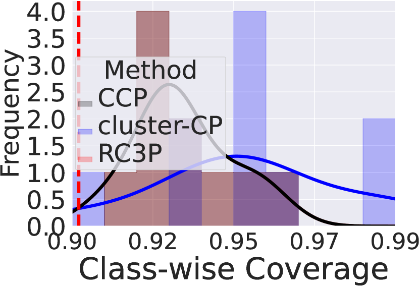
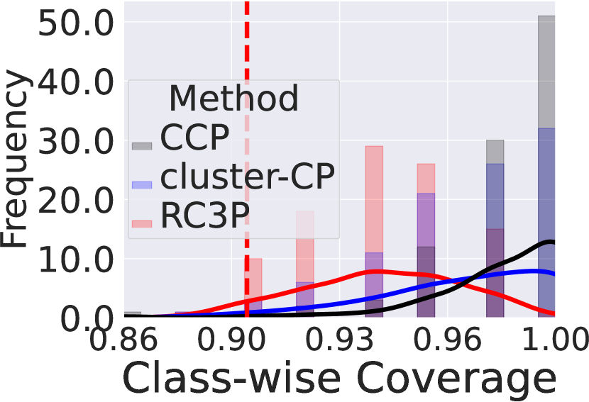
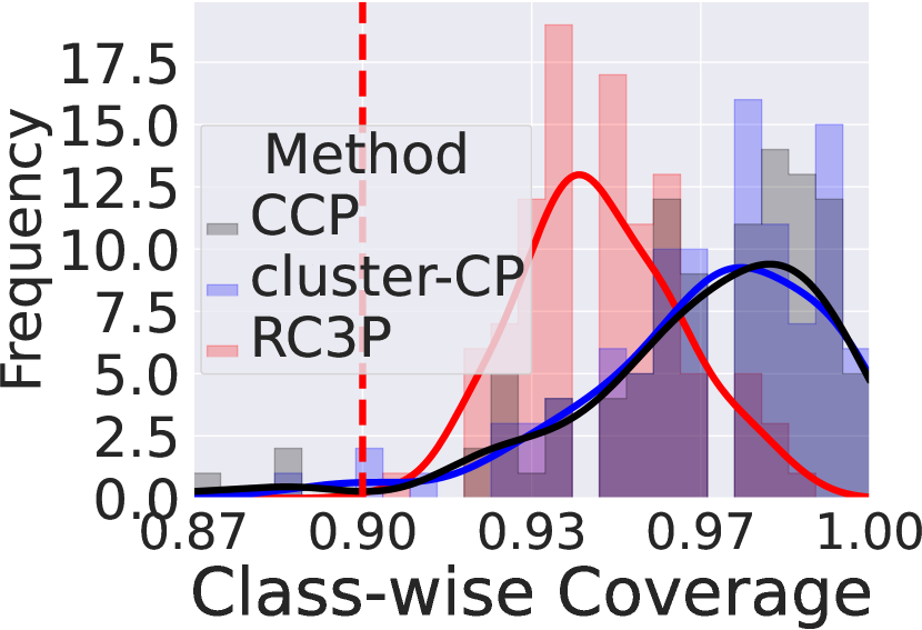
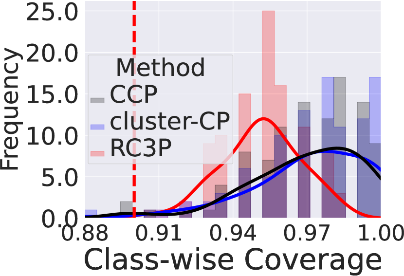
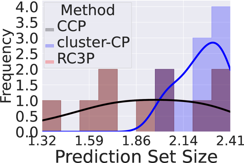
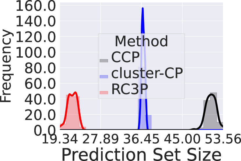
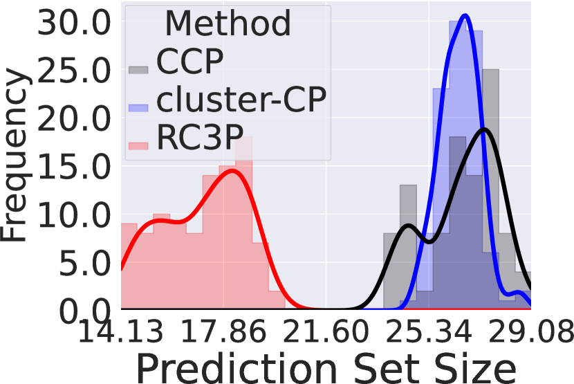
Figure 1: Class-conditional coverage (Top row) and prediction set size (Bottom row) achieved by CCP, Cluster-CP, and RC3P methods when $\alpha=0.1$ and models are trained with $200$ epochs on all four datasets with imbalance type EXP  $\rho=0.1$. We clarify that RC3P overlaps with CCP on CIFAR-10. It is clear that RC3P has more densely distributed class-conditional coverage above $0.9$ (the target $1-\alpha$ class-conditional coverage) than CCP and Cluster-CP with significantly smaller prediction sets on CIFAR-100, mini-ImageNet and Food-101.

(a) CIFAR-10

(b) CIFAR-100

(c) mini-ImageNet

(d) Food-101

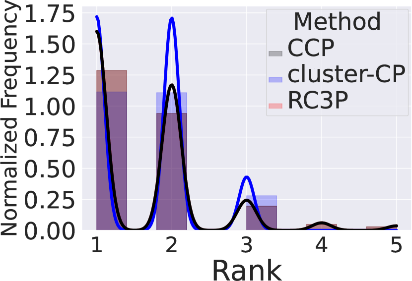
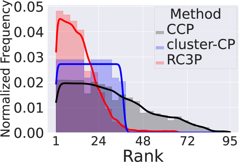
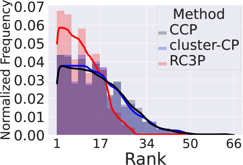
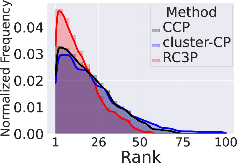
Figure 2: Visualization for the normalized frequency distribution of label ranks included in the prediction set of CCP, Cluster-CP, and RC3P with $\rho=0.1$ for imbalance type EXP when $\alpha=0.1$ and models are trained with $200$ epochs. It is clear that the distribution of normalized frequency generated by RC3P tends to be lower compared to those produced by CCP and Cluster-CP. Furthermore, the probability density function tail for label ranks in the RC3P prediction set is notably shorter than that of other methods.

RC3P significantly outperforms CCP and Cluster-CP. First, it is clear from Table B.4 and B.5 that RC3P, CCP, and Cluster-CP guarantee class-conditional coverage on all settings. This can also be observed by the first row of Fig 1, where the class-wise coverage bars of CCP and RC3P distribute on the right-hand side of the target probability $1-\alpha$ (red dashed line). Second, RC3P outperforms CCP and Cluster-CP with $26.25\%$ (on four datasets) or $35\%$ (excluding CIFAR-10) decrease in terms of average prediction set size the same class-wise coverage. We also report the histograms of the corresponding prediction set sizes in the second row of Figure 1, which shows (i) RC3P has more concentrated class-wise coverage distribution than CCP and Cluster-CP; (ii) the distribution of prediction set sizes produced by RC3P is globally smaller than that produced by CCP and Cluster-CP, which is justified by a better trade-off number of $\{\sigma_{y}\}_{y=1}^{K}$ as shown in Figure 3. We clarify that the class-wise coverage and the corresponding prediction set sizes RC3P overlap with CCP on CIFAR-10 in Figure 1.

Visualization of normalized frequency. Figure 2 illustrates the normalized frequency distribution of label ranks included in the prediction sets across various testing datasets. It is evident that the distribution of label ranks in the prediction set generated by RC3P tends to be lower compared to those produced by CCP and Cluster-CP. Furthermore, the probability density function tail for label ranks in the RC3P prediction set is notably shorter than that of other methods. This indicates that RC3P more effectively incorporates lower-ranked labels into prediction sets, as a result of its augmented rank calibration scheme.

(a) CIFAR-10

(b) CIFAR-100

(c) mini-ImageNet

(d) Food-101

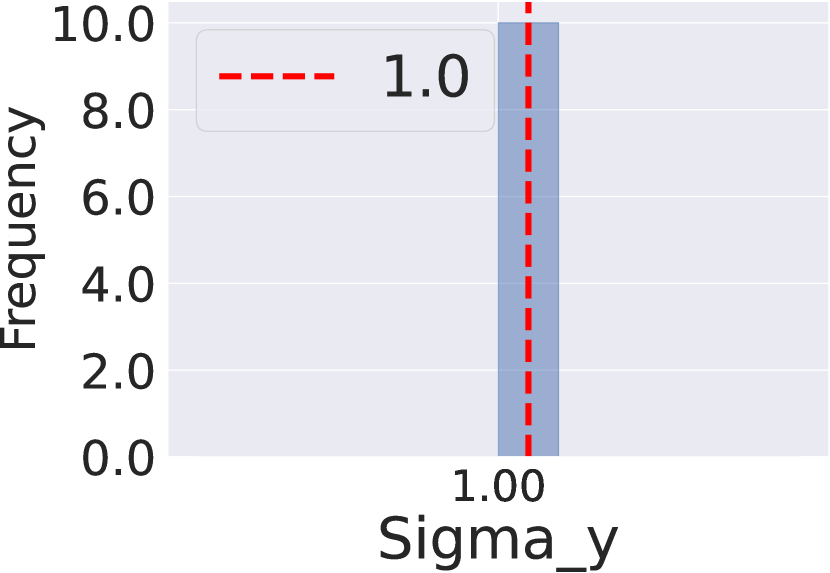
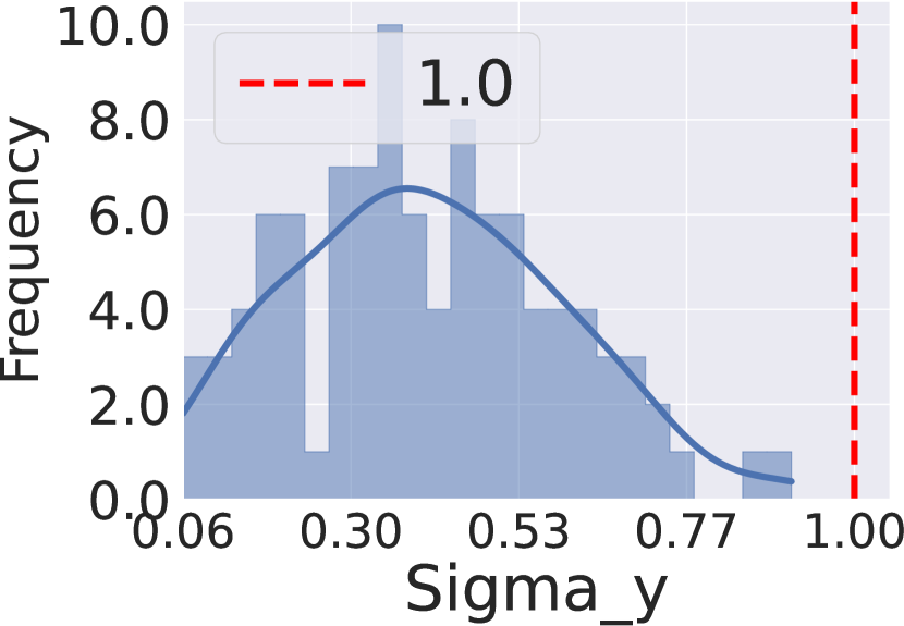
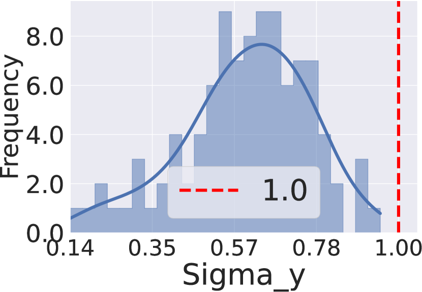
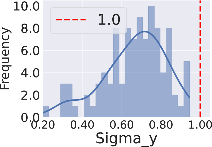
Figure 3: Verification of condition numbers $\{\sigma_{y}\}_{y=1}^{K}$ in Equation 6 with imbalance type EXP, $\rho=0.1$ when $\alpha=0.1$ and models are trained with $200$ epochs. Vertical dashed lines represent the value $1$, and we observe that all the condition numbers are smaller than $1$. This verifies the validity of the condition for Lemma 4.2, and thus confirms that RC3P produces smaller prediction sets than CCP using calibration on both non-conformity scores and label ranks.

Verification of $\sigma_{y}$. Figure 3 verifies the validity of Equation (6) on testing datasets and confirms the optimized trade-off between the coverage with inflated quantile and the constraint with calibrated label rank leads to smaller prediction sets. It also confirms that the condition number $\{\sigma_{y}\}_{y=1}^{K}$ could be evaluated on calibration datasets without testing datasets and thus decreases the overall computation cost. We verify $\sigma_{y}\leq 1$ for all settings and $\sigma_{y}$ is much smaller than $1$ on all datasets with large number of classes.

6 Summary

This paper studies a provable conformal prediction (CP) algorithm that aims to provide class-conditional coverage guarantee and to produce small prediction sets for imbalanced classification tasks. Our proposed RC3P algorithm performs double-calibration, one over conformity score and one over label rank for each class separately, to achieve this goal. Our experiments clearly demonstrate the significant efficacy of RC3P  over the baseline class-conditional CP algorithms.

Appendix A Technical Proofs of Theoretical Results

A.1 Proof of Theorem 4.1

Theorem A.1.

(Theorem 4.1 restated, class-conditional coverage of RC3P) Suppose that selecting $\widehat{k}(y)$ values result in the class-wise top-$k$ error $\epsilon_{y}^{\widehat{k}(y)}$ for each class $y\in\mathcal{Y}$. For a target class-conditional coverage $1-\alpha$, if we set $\widehat{\alpha}_{y}$ and $\widehat{k}(y)$ in RC3P  (3) in the following ranges:

$$\widehat{k}(y)\in\{k:\epsilon_{y}^{k}<\alpha\},\quad 0\leq\widehat{\alpha}_{y}\leq\alpha-\epsilon_{y}^{\widehat{k}(y)},$$ (8)

then RC3P can achieve the class-conditional coverage for every $y\in\mathcal{Y}$:

$$\mathbb{P}_{(X,Y)\sim\mathcal{P}}\{Y\in\widehat{\mathcal{C}}^{\text{RC3P}}_{1-\alpha}(X)|Y=y\}\geq 1-\alpha.$$

Proof.

(of Theorem 4.1)

Let $y\in\mathcal{Y}$ denote any class label. In this proof, we omit the superscript $k$ in the top-$k$ error notation $\epsilon_{y}^{k}$ for simplicity.

With the lower bound of the coverage on class $y$ (Theorem 1 in [9]), we have

$$1-\widehat{\alpha}\leq\mathbb{P}\{{Y_{\text{test}}}\in\widehat{\mathcal{C}}^{\text{CCP}}_{1-\widehat{\alpha}}({X_{\text{test}}})|Y=y\}$$

$$= \mathbb{P}\{V({X_{\text{test}}},{Y_{\text{test}}})\leq\widehat{Q}^{\text{class}}_{1-\widehat{\alpha}}(y)|Y=y\}$$

$$= \mathbb{P}\{V({X_{\text{test}}},{Y_{\text{test}}})\leq\widehat{Q}^{\text{class}}_{1-\hat{\alpha}}(y),r_{f}({X_{\text{test}}},{Y_{\text{test}}})\leq\widehat{k}(y)|Y=y\}$$

$$+\mathbb{P}\{V({X_{\text{test}}},{Y_{\text{test}}})\leq\widehat{Q}^{\text{class}}_{1-\hat{\alpha}}(y),r_{f}({X_{\text{test}}},{Y_{\text{test}}})>\widehat{k}(y)|Y=y\}$$

$$\leq \mathbb{P}\{V({X_{\text{test}}},{Y_{\text{test}}})\leq\widehat{Q}^{\text{class}}_{1-\hat{\alpha}}(y),r_{f}({X_{\text{test}}},{Y_{\text{test}}})\leq\widehat{k}(y)|Y=y\}$$

$$+\underbrace{\mathbb{P}\{r_{f}({X_{\text{test}}},{Y_{\text{test}}})>\widehat{k}(y)|Y=y\}}_{\leq\epsilon^{\widehat{k}(y)}_{y}}$$

$$\leq \mathbb{P}\{{Y_{\text{test}}}\in\widehat{\mathcal{C}}^{\text{RC3P}}_{1-\widehat{\alpha}}(y)|Y=y\}+\epsilon^{\widehat{k}(y)}_{y}.$$

Re-arranging the above inequality, we have

$$\mathbb{P}\{{Y_{\text{test}}}\in\widehat{\mathcal{C}}^{\text{RC3P}}_{1-\widehat{\alpha}}(y)|Y=y\}\geq 1-\widehat{\alpha}-\epsilon^{\widehat{k}(y)}_{y}\geq 1-\alpha,$$

where the last inequality is due to $\widehat{\alpha}_{y}\leq\alpha-\epsilon^{\widehat{k}(y)}_{y}$. This implies that RC3P guarantees the class-conditional coverage on any class $y$. This completes the proof for Theorem 4.1. ∎

A.2 Proof of Lemma 4.2

Theorem A.2.

(Lemma 4.2 restated, improved predictive efficiency of RC3P) Let $\widehat{\alpha}_{y}$ and $\widehat{k}(y)$ satisfy Theorem 4.1. If the following inequality holds for any $y\in\mathcal{Y}$:

$$\mathbb{P}_{X_{\text{test}}}\big{[}V({X_{\text{test}}},y)\leq\widehat{Q}^{\text{class}}_{1-\widehat{\alpha}}(y),~{}r_{f}({X_{\text{test}}},y)\leq\widehat{k}(y)\big{]}\leq\mathbb{P}_{X_{\text{test}}}\big{[}V({X_{\text{test}}},y)\leq\widehat{Q}^{\text{class}}_{1-\alpha}(y)\big{]},$$ (9)

then RC3P produces smaller expected prediction sets than CCP, i.e.,

$$\mathbb{E}_{X_{\text{test}}}[|\widehat{\mathcal{C}}^{\text{RC3P}}_{1-\widehat{\alpha}}({X_{\text{test}}})|]\leq\mathbb{E}_{X_{\text{test}}}[|\widehat{\mathcal{C}}^{\text{CCP}}_{1-\alpha}({X_{\text{test}}})|].$$

Proof.

(of Lemma 4.2)

The proof idea is to reduce the cardinality of the prediction set made by RC3P to that made by CCP in expectation. Let $\sigma_{y}=\frac{\mathbb{P}_{X_{\text{test}}}\Big{[}V({X_{\text{test}}},y)\leq\widehat{Q}^{\text{class}}_{1-\widehat{\alpha}}(y),~{}r_{f}({X_{\text{test}}},y)\leq\widehat{k}(y)\Big{]}}{\mathbb{P}_{X_{\text{test}}}\Big{[}V({X_{\text{test}}},y)\leq\widehat{Q}^{\text{class}}_{1-\alpha}(y)\Big{]}}.$ According to the assumption in (9), we know that $\sigma_{y}\leq 1$, which will be used later.

We start with the expected prediction set size of RC3Pand then derive its upper bound.

$$\mathbb{E}_{X_{\text{test}}}[|\widehat{\mathcal{C}}^{\text{RC3P}}_{1-\hat{\alpha}}({X_{\text{test}}})|]=\mathbb{E}_{X_{\text{test}}}\Bigg{[}\sum_{y\in\mathcal{Y}}\mathbbm{1}\Big{[}V({X_{\text{test}}},y)\leq\widehat{Q}^{\text{class}}_{1-\widehat{\alpha}}(y),~{}r_{f}({X_{\text{test}}},y)\leq\widehat{k}(y)\Big{]}\Bigg{]}$$

$$= \sum_{y\in\mathcal{Y}}\mathbb{E}_{X_{\text{test}}}\Big{[}\mathbbm{1}[V({X_{\text{test}}},y)\leq\widehat{Q}^{\text{class}}_{1-\widehat{\alpha}}(y),~{}r_{f}({X_{\text{test}}},y)\leq\widehat{k}(y)]\Big{]}$$

$$= \sum_{y\in\mathcal{Y}}\mathbb{P}_{X_{\text{test}}}\Big{[}V({X_{\text{test}}},y)\leq\widehat{Q}^{\text{class}}_{1-\widehat{\alpha}}(y),~{}r_{f}({X_{\text{test}}},y)\leq\widehat{k}(y)\Big{]}$$

$$\stackrel{{\scriptstyle(a)}}{{=}} \sum_{y\in\mathcal{Y}}\sigma_{y}\cdot\mathbb{P}_{X_{\text{test}}}\Big{[}V({X_{\text{test}}},y)\leq\widehat{Q}^{\text{class}}_{1-\alpha}(y)\Big{]}$$ (10)

$$\stackrel{{\scriptstyle(b)}}{{\leq}} \sum_{y\in\mathcal{Y}}\mathbb{E}_{X_{\text{test}}}\Big{[}\mathbbm{1}[V({X_{\text{test}}},y)\leq\widehat{Q}^{\text{class}}_{1-\alpha}(y)]\Big{]}$$

$$= \mathbb{E}_{X_{\text{test}}}\Bigg{[}\sum_{y\in\mathcal{Y}}\mathbbm{1}[V({X_{\text{test}}},y)\leq\widehat{Q}^{\text{class}}_{1-\alpha}(y)]\Bigg{]}=\mathbb{E}_{X_{\text{test}}}[|\widehat{\mathcal{C}}^{\text{CCP}}_{1-\alpha}({X_{\text{test}}})|],$$ (11)

where the equality $(a)$ is due to the definitions of $\sigma_{y}$, and inequality $(b)$ is due to the assumption

$$\sum_{y\in\mathcal{Y}}\sigma_{y}\cdot\mathbb{P}_{X_{\text{test}}}\Big{[}V({X_{\text{test}}},y)\leq\widehat{Q}^{\text{class}}_{1-\alpha}(y)\Big{]}\leq\sum_{y\in\mathcal{Y}}\mathbb{P}_{X_{\text{test}}}\Big{[}V({X_{\text{test}}},y)\leq\widehat{Q}^{\text{class}}_{1-\alpha}(y)\Big{]}.$$

This shows that RC3P requires smaller prediction sets to guarantee the class-conditional coverage compared to CCP. ∎

A.3 Proof of Theorem 4.3

Theorem A.3.

(Theorem 4.3 restated, conditions of improved predictive efficiency for RC3P) Define $D=\mathbb{P}[r_{f}(X,y)\leq\widehat{k}(y)|Y\neq y]$, and $\bar{r}_{f}(X,y)=\lfloor\frac{r_{f}(X,y)+1}{2}\rfloor$. Denote $B=\mathbb{P}[f(X)_{(\bar{r}_{f}(X,y))}\leq\widehat{Q}_{1-\alpha}^{\text{class}}(y)|Y\neq y]$ if $V$ is APS, or $B=\mathbb{P}[f(X)_{(\bar{r}_{f}(X,y))}+\lambda\leq\widehat{Q}_{1-\alpha}^{\text{class}}(y)|Y\neq y]$ if $V$ is RAPS. If $B-D\geq\frac{p_{y}}{1-p_{y}}(\alpha-\epsilon_{y}^{\widehat{k}(y)})$, then $\sigma_{y}\leq 1$.

Proof.

(of Theorem 4.3)

Based on the different choices of scoring function, we first divide two scenarios:

(i): If $V(X,y)$ is the APS scoring function, since the APS score cumulatively sums the ordered prediction of $f(X)$: $V(X,y)=\sum_{l=1}^{r_{f}(X,y)}f(X)_{(l)}$, it is easy to verify that $V(X,y)$ is concave in terms of $l$. As a result, we have

$$V(X,y)= \frac{r_{f}(X,y)}{r_{f}(X,y)}\cdot\sum_{l=1}^{r_{f}(X,y)}f(X)_{(l)}\leq r_{f}(X,y)\cdot f(X)_{(\lfloor\sum_{l=1}^{r_{f}(X,y)}l/r_{f}(X,y)\rfloor)}=r_{f}(X,y)\cdot f(X)_{(\bar{r}_{f}(X,y))},$$

where $\bar{r}_{f}(X,y)=\bigg{\lfloor}\frac{\sum_{l=1}^{r_{f}(X,y)}l}{r_{f}(X,y)}\bigg{\rfloor}=\lfloor(r_{f}(X,y)+1)/2\rfloor$.

Now we lower bound $\mathbb{P}_{X}[V(X,y)\leq\widehat{Q}_{1-\alpha}^{\text{class}}(y)]$ as follows.

$$\mathbb{P}_{X}[V(X,y)\leq\widehat{Q}_{1-\alpha}^{\text{class}}(y)]$$

$$= \underbrace{\mathbb{P}_{XY}[Y=y]}_{=p_{y}}\cdot\underbrace{\mathbb{P}_{X}[V(X,y)\leq\widehat{Q}_{1-\alpha}^{\text{class}}(y)|Y=y]}_{\geq 1-\alpha}+\underbrace{\mathbb{P}_{XY}[Y\neq y]}_{=1-p_{y}}\cdot\underbrace{\mathbb{P}_{X}[V(X,y)\leq\widehat{Q}_{1-\alpha}^{\text{class}}(y)|Y\neq y]}_{\geq B}$$

$$\geq p_{y}(1-\alpha)+(1-p_{y})B+p_{y}(1-\epsilon_{y}^{\widehat{k}(y)})+(1-p_{y})D-p_{y}(1-\epsilon_{y}^{\widehat{k}(y)})-(1-p_{y})D$$

$$\geq \mathbb{P}_{X}[r_{f}(X,y)\leq\widehat{k}(y)]-p_{y}(\alpha-\epsilon_{y}^{\widehat{k}(y)})+(1-p_{y})(B-D).$$ (12)

According to the assumption $B-D\geq\frac{p_{y}}{1-p_{y}}(\alpha-\epsilon_{y}^{\widehat{k}(y)})$, we have

$$\mathbb{P}_{X}[r_{f}(X,y)\leq\widehat{k}(y)]\leq\mathbb{P}_{X}[V(X,y)\leq\widehat{Q}_{1-\alpha}^{\text{class}}(y)].$$

(ii): If $V(X,y)$ is the RAPS scoring function and $r_{f}(X,y)\leq k_{reg}$, then the RAPS scoring function could be rewritten as: $V(X,y)=\sum_{l=1}^{r_{f}(X,y)}f(X)_{(l)}$. As a result, we have:

$$V(X,y)= \frac{r_{f}(X,y)}{r_{f}(X,y)}\cdot\sum_{l=1}^{r_{f}(X,y)}f(X)_{(l)}$$

$$\leq r_{f}(X,y)\cdot f(X)_{(\lfloor\sum_{l=1}^{r_{f}(X,y)}l/r_{f}(X,y)\rfloor)}$$

$$= r_{f}(X,y)\cdot f(X)_{(\bar{r}_{f}(X,y))}$$

$$\leq r_{f}(X,y)\cdot\Big{(}f(X)_{(\bar{r}_{f}(X,y))}+\lambda\Big{)}.$$

If $r_{f}(X,y)>k_{reg}$, then the RAPS scoring function could be rewritten as: $V(X,y)=\sum_{l=1}^{r_{f}(X,y)}f(X)_{(l)}+\lambda(r_{f}(X,y)-k_{reg})$. As a result, we have

$$V(X,y) =\frac{r_{f}(X,y)}{r_{f}(X,y)}\cdot\Big{(}\sum_{l=1}^{r_{f}(X,y)}f(X)_{(l)}+\lambda\big{(}r_{f}(X,y)-k_{reg}\big{)}\Big{)}$$

$$\leq r_{f}(X,y)\cdot\Big{(}f(X)_{(\bar{r}_{f}(X,y))}+\lambda\big{(}1-\frac{k_{reg}}{r_{f}(X,y)}\big{)}\Big{)}$$

$$\leq r_{f}(X,y)\cdot\Big{(}f(X)_{(\bar{r}_{f}(X,y))}+\lambda\Big{)}.$$

Then, by applying the Inequality A.3, we have:

$$\mathbb{P}_{X}[r_{f}(X,y)\leq\widehat{k}(y)]\leq\mathbb{P}_{X}[V(X,y)\leq\widehat{Q}_{1-\alpha}^{\text{class}}(y)].$$

This completes the proof for Theorem 4.3. ∎

Appendix B Complete Experimental Results

B.1 Training Details

For CIFAR-10 and CIFAR-100, we train ResNet20 using LDAM loss function given in [5] with standard mini-batch stochastic gradient descent (SGD) using learning rate $0.1$, momentum $0.9$, and weight decay $2e-4$ for $200$ epochs and $50$ epochs. The batch size is $128$. For experiments on mini-ImageNet, we use the same setting. For Food-101, the batch size is $256$ and other parameters are kept the same. We reported our main results when models were trained in $200$ epochs. Other results are reported in Appendix B.7 and Table B.7.

We also evaluate the top-1 accuracy over the majority, medium, and minority groups of classes as the class-wise performance when $200$ epochs. To show the variation of class-wise performance, we divide some classes with the largest number of data samples into the majority group, and the number of these classes is a quarter ($25\%$) of the total number of classes. Similarly, we divide the classes with the smallest number of data into the minority group ($25\%$) and the remaining classes as the medium group ($50\%$). In the above table, we show the accuracy of three groups with three imbalance types and two imbalance ratios $\rho=0.1,\rho=0.5$ on four datasets.

The results are summarized in Table B.1. As can be seen, the group-wise performance can vary significantly from high to very low. The class-imbalance setting is the case where the classifier does not perform very well in some classes.

Table 3: Top-1 accuracy of minority, medium, and majority groups with three imbalance types and two imbalance ratios $\rho=0.1,\rho=0.5$ on four datasets. We could observe that the class-wise performance varies significantly over different classes.

@c! cc! cc! cc@ 2-1Groups 1-2EXP 1-2POLY 1-2MAJ
$\rho$ = 0.5 $\rho$ = 0.1 $\rho$ = 0.5 $\rho$ = 0.1 $\rho$ = 0.5 $\rho$ = 0.1
1-*CIFAR-10
Minority 0.913 0.961 0.932 0.901 0.940 0.927
Medium 0.872 0.822 0.867 0.847 0.848 0.75
Majority 0.949 0.832 0.933 0.948 0.914 0.795
1-*CIFAR-100
Minority 0.554 0.295 0.468 0.352 0.572 0.365
Medium 0.589 0.536 0.517 0.413 0.574 0.476
Majority 0.668 0.720 0.671 0.588 0.616 0.562
1-*mini-ImageNet
Minority 0.677 0.640 0.624 0.627 0.626 0.642
Medium 0.527 0.546 0.533 0.530 0.526 0.538
Majority 0.633 0.679 0.684 0.67 0.673 0.686
1-*Food-101
Minority 0.453 0.231 0.379 0.289 0.505 0.333
Medium 0.579 0.474 0.496 0.398 0.579 0.467
Majority 0.582 0.660 0.596 0.563 0.532 0.490

B.2 Calibration Details

As mentioned in Section 5.1, we balanced split the validation set of CIFAR-10 and CIFAR-100, the number of calibration data is $5000$. For mini-ImageNet, the number of calibration data is $15000$. For Food-101, the total number is $12625$. To compute the mean and standard deviation for the overall performance, we repeat calibration experiments for $10$ times. In our main results, We set $\alpha=0.1$. We also report other experiment results of different $\alpha$ values, $\alpha=0.05$ and $\alpha=0.01$, in Appendix B.6, and Table B.6 and B.6.

The regularization parameter for RAPS scoring function is from the set $k_{reg}\in\{3,5,7\}$ and $\lambda\in\{0.001,0.01,0.1\}$ based on the empirical setting in cluster-CP. We select the combination of $k_{reg}$ and $\lambda$ for each experiment with the same imbalanced type and imbalanced ratio on the same dataset, where most of the APSS values of all methods are minimum.

The hyper-parameter $g$ is selected from the set $\{0.25,0.5,0.75,1.0\}$ to find the minimal $g$ that CCP, Cluster-CP , and RC3P achieve the target class-conditional coverage. We clarify that for each dataset and each class-conditional CP method, we use fixed $g$ values. The detailed $g$ values are displayed in Table B.2. From Table B.2, we could observe that the hyperparameter $g$ for RC3P is always smaller than other methods, which means that comparing other class-wise CP algorithms, our algorithm needs the smallest inflation on $1-\widehat{\alpha}$ to achieve the target class-conditional coverage. This could also match the result of histograms of class-conditional coverage.

Table 4: Hyperparameter $g$ choices for each class-conditional CP methods CCP, Cluster-CP, and RC3P on four datasets CIFAR-10, CIFAR-100, mini-ImageNet, and Food101. We could observe that all $g$ values are in constant order to make a fair comparison. Meanwhile, the hyperparameter $g$ for RC3P is always smaller than other methods.

@c! cccc@ 2-1Methods 1-*Dataset
CIFAR-10 CIFAR-100 mini-ImageNet FOOD-101

CCP 0.5 0.5 0.75 0.75
Cluster-CP 1.0 0.5 0.75 0.75
RC3P 0.5 0.25 0.5 0.5

B.3 Illustration of Imbalanced Data

(a) EXP

(b) POLY

(c) MAJ

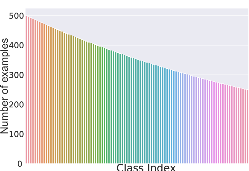
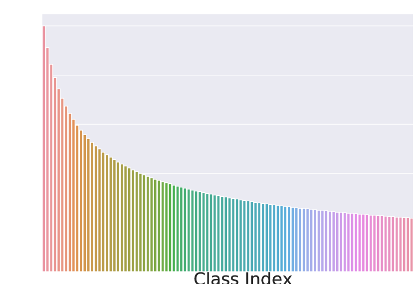
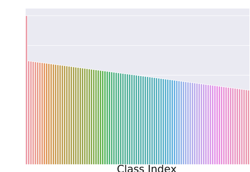
Figure 4: Illustrative examples of the different imbalanced distributions of the number of training examples per class index $c$ on CIFAR-100

B.4 Comparison Experiments Using APS Score Function

Based on the results in Table B.4, we make the following observations: (i) CCP, Cluster-CP, and RC3P can guarantee the class-conditional coverage; and (ii) RC3P significantly outperforms CCP and Cluster-CCP on three datasets by producing smaller prediction sets.

Table 5: Results comparing CCP, Cluster-CP, and RC3P with ResNet-20 model and APS scoring function under different imbalance ratios $\rho=0.5$ and $\rho=0.1$ when $\alpha=0.1$. We set UCR of RC3P the same as or better than that of CCP and Cluster-CP for a fair comparison of prediction set size. The APSS results show that RC3P significantly outperforms Cluster-CP in terms of the average prediction set size over all settings on CIFAR-100, mini-ImageNet, and Food-101.

@cc! cc! cc! cc@ 2-1Measure 2-1Methods 1-2EXP 1-2POLY 1-2MAJ
$\rho$ = 0.5 $\rho$ = 0.1 $\rho$ = 0.5 $\rho$ = 0.1 $\rho$ = 0.5 $\rho$ = 0.1
1-*CIFAR-10
3-1UCR CCP 0.050 $\pm$ 0.016 0.100 $\pm$ 0.020 0.100 $\pm$ 0.032 0.050 $\pm$ 0.021 0.070 $\pm$ 0.014 0.040 $\pm$ 0.015
Cluster-CP 0.010 $\pm$ 0.009 0.090 $\pm$ 0.009 0.080 $\pm$ 0.019 0.060 $\pm$ 0.001 0.020 $\pm$ 0.012 0.070 $\pm$ 0.014
RC3P 0.050 $\pm$ 0.016 0.100 $\pm$ 0.020 0.100 $\pm$ 0.032 0.050 $\pm$ 0.021 0.070 $\pm$ 0.014 0.040 $\pm$ 0.015
3-1APSS CCP 1.555 $\pm$ 0.010 1.855 $\pm$ 0.014 1.538 $\pm$ 0.010 1.776 $\pm$ 0.012 1.840 $\pm$ 0.020 2.629 $\pm$ 0.013
Cluster-CP 1.714 $\pm$ 0.018 2.162 $\pm$ 0.015 1.706 $\pm$ 0.014 1.928 $\pm$ 0.013 1.948 $\pm$ 0.023 3.220 $\pm$ 0.020
RC3P 1.555 $\pm$ 0.010 1.855 $\pm$ 0.014 1.538 $\pm$ 0.010 1.776 $\pm$ 0.012 1.840 $\pm$ 0.020 2.629 $\pm$ 0.013
1-*CIFAR-100
3-1UCR CCP 0.007 $\pm$ 0.002 0.010 $\pm$ 0.002 0.010 $\pm$ 0.002 0.014 $\pm$ 0.003 0.016 $\pm$ 0.003 0.008 $\pm$ 0.004
Cluster-CP 0.012 $\pm$ 0.002 0.016 $\pm$ 0.004 0.020 $\pm$ 0.003 0.004 $\pm$ 0.002 0.016 $\pm$ 0.003 0.019 $\pm$ 0.005
RC3P 0.005 $\pm$ 0.002 0.011 $\pm$ 0.002 0.009 $\pm$ 0.003 0.015 $\pm$ 0.003 0.008 $\pm$ 0.002 0.008 $\pm$ 0.004
3-1APSS CCP 44.224 $\pm$ 0.341 50.969 $\pm$ 0.345 49.889 $\pm$ 0.353 64.343 $\pm$ 0.237 44.194 $\pm$ 0.514 64.642 $\pm$ 0.535
Cluster-CP 29.238 $\pm$ 0.609 37.592 $\pm$ 0.857 38.252 $\pm$ 0.353 52.391 $\pm$ 0.595 31.518 $\pm$ 0.335 50.883 $\pm$ 0.673
RC3P 17.705 $\pm$ 0.004 21.954 $\pm$ 0.005 23.048 $\pm$ 0.008 33.185 $\pm$ 0.005 18.581 $\pm$ 0.007 32.699 $\pm$ 0.005
1-*mini-ImageNet
3-1UCR CCP 0.008 $\pm$ 0.004 0.008 $\pm$ 0.004 0.005 $\pm$ 0.002 0.004 $\pm$ 0.001 0.010 $\pm$ 0.004 0.005 $\pm$ 0.002
Cluster-CP 0.014 $\pm$ 0.004 0.012 $\pm$ 0.004 0.011 $\pm$ 0.003 0.014 $\pm$ 0.003 0.008 $\pm$ 0.002 0.010 $\pm$ 0.003
RC3P 0.000 $\pm$ 0.000 0.001 $\pm$ 0.001 0.000 $\pm$ 0.000 0.000 $\pm$ 0.000 0.000 $\pm$ 0.000 0.000 $\pm$ 0.000
3-1APSS CCP 26.676 $\pm$ 0.171 26.111 $\pm$ 0.194 26.626 $\pm$ 0.133 26.159 $\pm$ 0.208 27.313 $\pm$ 0.154 25.629 $\pm$ 0.207
Cluster-CP 25.889 $\pm$ 0.301 25.253 $\pm$ 0.346 26.150 $\pm$ 0.393 25.633 $\pm$ 0.268 26.918 $\pm$ 0.241 25.348 $\pm$ 0.334
RC3P 18.129 $\pm$ 0.003 17.082 $\pm$ 0.002 17.784 $\pm$ 0.003 17.465 $\pm$ 0.003 18.111 $\pm$ 0.002 17.167 $\pm$ 0.004
1-*Food-101
3-1UCR CCP 0.006 $\pm$ 0.002 0.006 $\pm$ 0.002 0.009 $\pm$ 0.003 0.008 $\pm$ 0.001 0.006 $\pm$ 0.001 0.008 $\pm$ 0.002
Cluster-CP 0.003 $\pm$ 0.002 0.009 $\pm$ 0.003 0.004 $\pm$ 0.001 0.009 $\pm$ 0.002 0.011 $\pm$ 0.003 0.011 $\pm$ 0.002
RC3P 0.000 $\pm$ 0.000 0.000 $\pm$ 0.000 0.000 $\pm$ 0.000 0.001 $\pm$ 0.001 0.000 $\pm$ 0.000 0.000 $\pm$ 0.000
3-1APSS CCP 27.022 $\pm$ 0.192 30.900 $\pm$ 0.170 30.943 $\pm$ 0.119 35.912 $\pm$ 0.105 27.415 $\pm$ 0.194 36.776 $\pm$ 0.132
Cluster-CP 28.953 $\pm$ 0.333 33.375 $\pm$ 0.377 33.079 $\pm$ 0.393 38.301 $\pm$ 0.232 30.071 $\pm$ 0.412 39.632 $\pm$ 0.342
RC3P 18.369 $\pm$ 0.004 21.556 $\pm$ 0.006 21.499 $\pm$ 0.003 25.853 $\pm$ 0.004 19.398 $\pm$ 0.006 26.585 $\pm$ 0.004

B.5 Comparison Experiments Using RAPS Score Function

With the same model, evaluation metrics, and RAPS score function [20], we add the comparison experiments with CCP, and Cluster-CP on four datasets with different imbalanced types and imbalance ratio $\rho=0.5$ and $\rho=0.1$. The regularization parameter for RAPS scoring function is from the set $k_{reg}\in\{3,5,7\}$ and $\lambda\in\{0.001,0.01,0.1\}$. We select the combination of $k_{reg}$ and $\lambda$ for each experiment with the same imbalanced type and imbalanced ratio on the same dataset, where most of the $APSS$ values of all methods are minimum. The overall performance is summarized in Table B.5. We highlight that we also select the $g$ from the set $g\in\{0.25,0.5,0.75,1.0\}$ to find the minimal $g$ that CCP, Cluster-CP, and RC3P approximately achieves the target class conditional coverage.

Based on the results in Table B.5, we make the following observations: (i) CCP, Cluster-CP, and RC3P can guarantee the class-conditional coverage; and (ii) RC3P significantly outperforms CCP and Cluster-CP on three datasets by producing smaller prediction sets.

Table 6: Results comparing CCP, Cluster-CP, and RC3P with ResNet-20 model and the RAPS scoring function under different imbalance ratios $\rho=0.5$ and $\rho=0.1$ when $\alpha=0.1$. The regularization parameter for RAPS scoring function is selected from the set $[3,5,7]$ and $[0.001,0.01,0.1]$. We select the best results for each element in the table. We set UCR of RC3P the same as or better than that of CCP and Cluster-CP for a fair comparison of prediction set size. The APSS results show that RC3P significantly outperforms CCP and Cluster-CP in terms of average prediction set size over all settings on CIFAR-100, mini-ImageNet, and Food-101.

@cc! cc! cc! cc@ 2-1Measure 2-1Methods 1-2EXP 1-2POLY 1-2MAJ
$\rho$ = 0.5 $\rho$ = 0.1 $\rho$ = 0.5 $\rho$ = 0.1 $\rho$ = 0.5 $\rho$ = 0.1
1-*CIFAR-10
3-1UCR CCP 0.050 $\pm$ 0.016 0.010 $\pm$ 0.020 0.100 $\pm$ 0.028 0.050 $\pm$ 0.021 0.070 $\pm$ 0.014 0.040 $\pm$ 0.015
Cluster-CP 0.010 $\pm$ 0.009 0.010 $\pm$ 0.010 0.080 $\pm$ 0.019 0.060 $\pm$ 0.015 0.020 $\pm$ 0.025 0.070 $\pm$ 0.014
RC3P 0.050 $\pm$ 0.016 0.010 $\pm$ 0.020 0.100 $\pm$ 0.028 0.050 $\pm$ 0.021 0.070 $\pm$ 0.014 0.040 $\pm$ 0.015
3-1APSS CCP 1.555 $\pm$ 0.010 1.855 $\pm$ 0.014 1.538 $\pm$ 0.010 1.776 $\pm$ 0.012 1.840 $\pm$ 0.020 2.632 $\pm$ 0.012
Cluster-CP 1.714 $\pm$ 0.018 2.162 $\pm$ 0.015 1.706 $\pm$ 0.014 1.929 $\pm$ 0.013 1.787 $\pm$ 0.019 2.968 $\pm$ 0.024
RC3P 1.555 $\pm$ 0.010 1.855 $\pm$ 0.014 1.538 $\pm$ 0.010 1.776 $\pm$ 0.012 1.840 $\pm$ 0.020 2.632 $\pm$ 0.012
1-*CIFAR-100
3-1UCR CCP 0.007 $\pm$ 0.002 0.011 $\pm$ 0.002 0.010 $\pm$ 0.002 0.015 $\pm$ 0.003 0.015 $\pm$ 0.003 0.008 $\pm$ 0.004
Cluster-CP 0.012 $\pm$ 0.002 0.017 $\pm$ 0.004 0.019 $\pm$ 0.004 0.034 $\pm$ 0.005 0.008 $\pm$ 0.003 0.018 $\pm$ 0.006
RC3P 0.005 $\pm$ 0.002 0.011 $\pm$ 0.002 0.009 $\pm$ 0.003 0.015 $\pm$ 0.003 0.015 $\pm$ 0.003 0.008 $\pm$ 0.004
3-1APSS CCP 44.250 $\pm$ 0.342 50.970 $\pm$ 0.345 49.886 $\pm$ 0.353 64.332 $\pm$ 0.236 48.343 $\pm$ 0.353 64.663 $\pm$ 0.535
Cluster-CP 29.267 $\pm$ 0.612 37.795 $\pm$ 0.862 38.258 $\pm$ 0.320 52.374 $\pm$ 0.592 31.513 $\pm$ 0.325 50.379 $\pm$ 0.684
RC3P 17.705 $\pm$ 0.004 21.954 $\pm$ 0.005 23.048 $\pm$ 0.008 33.185 $\pm$ 0.005 18.581 $\pm$ 0.006 32.699 $\pm$ 0.006
1-*mini-ImageNet
3-1UCR CCP 0.008 $\pm$ 0.003 0.009 $\pm$ 0.004 0.005 $\pm$ 0.002 0.004 $\pm$ 0.002 0.009 $\pm$ 0.003 0.005 $\pm$ 0.002
Cluster-CP 0.006 $\pm$ 0.002 0.013 $\pm$ 0.005 0.009 $\pm$ 0.003 0.016 $\pm$ 0.001 0.007 $\pm$ 0.002 0.009 $\pm$ 0.004
RC3P 0.000 $\pm$ 0.000 0.001 $\pm$ 0.001 0.000 $\pm$ 0.000 0.000 $\pm$ 0.000 0.000 $\pm$ 0.000 0.000 $\pm$ 0.000
3-1APSS CCP 26.756 $\pm$ 0.178 26.212 $\pm$ 0.199 26.689 $\pm$ 0.142 26.248 $\pm$ 0.219 27.397 $\pm$ 0.162 25.725 $\pm$ 0.214
Cluster-CP 26.027 $\pm$ 0.325 25.415 $\pm$ 0.289 26.288 $\pm$ 0.407 25.712 $\pm$ 0.315 26.969 $\pm$ 0.305 25.532 $\pm$ 0.350
RC3P 18.129 $\pm$ 0.003 17.082 $\pm$ 0.002 17.784 $\pm$ 0.003 17.465 $\pm$ 0.003 18.111 $\pm$ 0.002 17.167 $\pm$ 0.004
1-*Food-101
3-1UCR CCP 0.006 $\pm$ 0.003 0.006 $\pm$ 0.002 0.009 $\pm$ 0.003 0.008 $\pm$ 0.001 0.006 $\pm$ 0.002 0.008 $\pm$ 0.002
Cluster-CP 0.004 $\pm$ 0.003 0.012 $\pm$ 0.004 0.006 $\pm$ 0.002 0.006 $\pm$ 0.003 0.011 $\pm$ 0.003 0.014 $\pm$ 0.004
RC3P 0.000 $\pm$ 0.000 0.000 $\pm$ 0.000 0.000 $\pm$ 0.000 0.001 $\pm$ 0.001 0.000 $\pm$ 0.000 0.000 $\pm$ 0.000
3-1APSS CCP 27.022 $\pm$ 0.192 30.900 $\pm$ 0.170 30.966 $\pm$ 0.125 35.940 $\pm$ 0.111 27.439 $\pm$ 0.203 36.802 $\pm$ 0.138
Cluster-CP 28.953 $\pm$ 0.333 33.375 $\pm$ 0.377 33.337 $\pm$ 0.409 38.499 $\pm$ 0.216 29.946 $\pm$ 0.407 39.529 $\pm$ 0.306
RC3P 18.369 $\pm$ 0.004 21.556$\pm$ 0.006 21.499 $\pm$ 0.003 25.853 $\pm$ 0.004 19.397 $\pm$ 0.006 26.585 $\pm$ 0.004

B.6 Comparison Experiments with different $\alpha$ values

With the same model, evaluation metrics, and scoring functions, we add the comparison experiments with CCP, and Cluster-CP on four datasets with different imbalanced types and imbalance ratio $\rho=0.5$ and $\rho=0.1$ under the different $\alpha$ values. The overall performance is summarized in Table B.6 and B.6, with $\alpha=0.05$ and $\alpha=0.01$, respectively. We highlight that we also select the $g$ from the set $g\in[0.15,0.75]$ with $0.05$ range to find the minimal $g$ that CCP, Cluster-CP, and RC3P approximately achieves the target class conditional coverage.

Based on the results in Table B.5, we make the following observations: (i) CCP, Cluster-CP, and RC3P can guarantee the class-conditional coverage; and (ii) RC3P significantly outperforms CCP and Cluster-CP on three datasets by producing smaller prediction sets.

Table 7: APSS results comparing CCP, Cluster-CP, and RC3P with ResNet-20 model under different imbalance ratio $\rho=0.5$ and $\rho=0.1$ where $\alpha=0.05$. For a fair comparison of prediction set size, we set UCR of RC3P the same as or smaller (more restrictive) than that of CCP and Cluster-CP under $0.16$ on CIFAR-10 and $0.03$ on other datasets. The APSS results show that RC3P significantly outperforms CCP and Cluster-CP in terms of average prediction set size with $21.036\%$ (four datasets) or $28.048\%$ (excluding CIFAR-10) reduction in prediction size on average over $\text{min}\{\texttt{CCP},\texttt{cluster-CP}\}$.

@cc! cc! cc! cc@ 2-1Conformity Score 2-1Methods 1-2EXP 1-2POLY 1-2MAJ
$\rho$ = 0.5 $\rho$ = 0.1 $\rho$ = 0.5 $\rho$ = 0.1 $\rho$ = 0.5 $\rho$ = 0.1
1-*CIFAR-10
3-1APS CCP 2.861 $\pm$ 0.027 3.496 $\pm$ 0.037 2.744 $\pm$ 0.033 3.222 $\pm$ 0.018 3.269 $\pm$ 0.037 4.836 $\pm$ 0.035
Cluster-CP 3.443 $\pm$ 0.041 4.551 $\pm$ 0.049 3.309 $\pm$ 0.037 4.012 $\pm$ 0.039 4.075 $\pm$ 0.069 5.958 $\pm$ 0.070
RC3P 2.861 $\pm$ 0.027 3.496 $\pm$ 0.037 2.744 $\pm$ 0.033 3.222 $\pm$ 0.018 3.269 $\pm$ 0.037 4.836 $\pm$ 0.035
3-1RAPS CCP 2.833 $\pm$ 0.018 3.448 $\pm$ 0.036 2.774 $\pm$ 0.033 3.231 $\pm$ 0.021 3.301 $\pm$ 0.024 4.842 $\pm$ 0.037
Cluster-CP 3.430 $\pm$ 0.044 4.389 $\pm$ 0.062 3.352 $\pm$ 0.035 3.876 $\pm$ 0.034 4.044 $\pm$ 0.055 5.959 $\pm$ 0.083
RC3P 2.833 $\pm$ 0.018 3.448 $\pm$ 0.036 2.774 $\pm$ 0.033 3.231 $\pm$ 0.021 3.301 $\pm$ 0.024 4.842 $\pm$ 0.037
1-*CIFAR-100
3-1APS CCP 44.019 $\pm$ 0.295 51.004 $\pm$ 0.366 49.564 $\pm$ 0.315 64.314 $\pm$ 0.231 48.024 $\pm$ 0.386 64.941 $\pm$ 0.532
Cluster-CP 39.641 $\pm$ 0.567 46.746 $\pm$ 0.147 47.654 $\pm$ 0.371 62.340 $\pm$ 0.404 37.634 $\pm$ 0.537 60.841 $\pm$ 0.391
RC3P 32.128 $\pm$ 0.011 38.769 $\pm$ 0.006 39.930 $\pm$ 0.008 53.147 $\pm$ 0.010 34.361 $\pm$ 0.007 51.498 $\pm$ 0.009
3-1RAPS CCP 44.234 $\pm$ 0.341 50.950 $\pm$ 0.344 49.889 $\pm$ 0.355 64.339 $\pm$ 0.236 48.310 $\pm$ 0.353 64.628 $\pm$ 0.535
Cluster-CP 39.212 $\pm$ 0.365 46.840 $\pm$ 0.186 49.094 $\pm$ 0.280 62.095 $\pm$ 0.278 41.596 $\pm$ 0.323 60.158 $\pm$ 0.536
RC3P 32.135 $\pm$ 0.010 38.793 $\pm$ 0.007 39.871 $\pm$ 0.010 53.169 $\pm$ 0.009 34.380 $\pm$ 0.007 51.512 $\pm$ 0.008
1-*mini-ImageNet
3-1APS CCP 58.527 $\pm$ 0.445 57.527 $\pm$ 0.408 60.327 $\pm$ 0.520 56.581 $\pm$ 0.438 59.360 $\pm$ 0.430 56.636 $\pm$ 0.469
Cluster-CP 47.613 $\pm$ 0.544 46.650 $\pm$ 0.699 47.117 $\pm$ 0.930 45.360 $\pm$ 0.582 59.002 $\pm$ 0.434 56.147 $\pm$ 0.456
RC3P 32.046 $\pm$ 0.002 31.729 $\pm$ 0.003 31.718 $\pm$ 0.004 32.048 $\pm$ 0.003 32.909 $\pm$ 0.007 31.441 $\pm$ 0.004
3-1RAPS CCP 58.615 $\pm$ 0.428 57.626 $\pm$ 0.394 60.173 $\pm$ 0.527 56.702 $\pm$ 0.414 59.532 $\pm$ 0.430 56.903 $\pm$ 0.460
Cluster-CP 47.427 $\pm$ 0.588 46.767 $\pm$ 0.724 47.302 $\pm$ 1.126 45.603 $\pm$ 0.639 59.408 $\pm$ 0.482 56.779 $\pm$ 0.486
RC3P 32.040 $\pm$ 0.003 31.741 $\pm$ 0.003 31.752 $\pm$ 0.003 32.067 $\pm$ 0.002 32.914 $\pm$ 0.005 31.417 $\pm$ 0.005
1-*Food-101
3-1APS CCP 55.967 $\pm$ 0.464 60.374 $\pm$ 0.383 60.717 $\pm$ 0.596 65.698 $\pm$ 0.405 56.934 $\pm$ 0.446 66.654 $\pm$ 0.511
Cluster-CP 48.699 $\pm$ 0.512 55.288 $\pm$ 0.815 54.063 $\pm$ 0.885 60.104 $\pm$ 0.608 48.894 $\pm$ 0.919 59.432 $\pm$ 0.754
RC3P 31.224 $\pm$ 0.004 35.273 $\pm$ 0.007 35.364 $\pm$ 0.003 41.109 $\pm$ 0.005 31.661 $\pm$ 0.005 39.135 $\pm$ 0.003
3-1RAPS CCP 55.872 $\pm$ 0.465 60.764 $\pm$ 0.394 60.618 $\pm$ 0.579 65.681 $\pm$ 0.401 56.982 $\pm$ 0.447 66.615 $\pm$ 0.504
Cluster-CP 48.371 $\pm$ 0.513 55.155 $\pm$ 0.775 53.813 $\pm$ 0.864 59.912 $\pm$ 0.530 49.259 $\pm$ 0.846 59.307 $\pm$ 0.648
RC3P 31.229 $\pm$ 0.004 35.283 $\pm$ 0.006 35.379 $\pm$ 0.003 41.113 $\pm$ 0.005 31.631 $\pm$ 0.004 39.118 $\pm$ 0.003

Table 8: APSS results comparing CCP, Cluster-CP, and RC3P with ResNet-20 model under different imbalance ratio $\rho=0.5$ and $\rho=0.1$ where $\alpha=0.01$. For a fair comparison of prediction set size, we set UCR of RC3P the same as or smaller (more restrictive) than that of CCP and Cluster-CP under $0.16$ on CIFAR-10 and $0.03$ on other datasets. The APSS results show that RC3P significantly outperforms CCP and Cluster-CP in terms of average prediction set size with $16.911\%$ (four datasets) or $22.549\%$ (excluding CIFAR-10) reduction in prediction size on average over $\text{min}\{\texttt{CCP},\texttt{cluster-CP}\}$.

@cc! cc! cc! cc@ 2-1Conformity Score 2-1Methods 1-2EXP 1-2POLY 1-2MAJ
$\rho$ = 0.5 $\rho$ = 0.1 $\rho$ = 0.5 $\rho$ = 0.1 $\rho$ = 0.5 $\rho$ = 0.1
1-*CIFAR-10
3-1APS CCP 7.250 $\pm$ 0.164 7.387 $\pm$ 0.116 7.173 $\pm$ 0.079 7.596 $\pm$ 0.109 7.392 $\pm$ 0.128 8.864 $\pm$ 0.108
Cluster-CP 5.528 $\pm$ 0.103 8.332 $\pm$ 0.060 6.954 $\pm$ 0.084 7.762 $\pm$ 0.143 7.586 $\pm$ 0.113 9.308 $\pm$ 0.054
RC3P 5.671 $\pm$ 0.046 7.387 $\pm$ 0.116 6.309 $\pm$ 0.042 7.276 $\pm$ 0.010 6.779 $\pm$ 0.013 8.864 $\pm$ 0.108
3-1RAPS CCP 7.294 $\pm$ 0.160 7.458 $\pm$ 0.101 7.067 $\pm$ 0.106 7.597 $\pm$ 0.096 7.547 $\pm$ 0.134 8.884 $\pm$ 0.106
Cluster-CP 5.568 $\pm$ 0.103 8.288 $\pm$ 0.118 6.867 $\pm$ 0.078 7.795 $\pm$ 0.136 7.813 $\pm$ 0.142 9.239 $\pm$ 0.055
RC3P 5.673 $\pm$ 0.040 7.458 $\pm$ 0.101 6.310 $\pm$ 0.046 7.253 $\pm$ 0.006 6.780 $\pm$ 0.015 8.884 $\pm$ 0.106
1-*CIFAR-100
3-1APS CCP 100.0 $\pm$ 0.0 100.0 $\pm$ 0.0 100.0 $\pm$ 0.0 100.0 $\pm$ 0.0 100.0 $\pm$ 0.0 100.0 $\pm$ 0.0
Cluster-CP 65.523 $\pm$ 0.495 69.063 $\pm$ 0.512 67.012 $\pm$ 0.739 81.997 $\pm$ 0.390 100.0 $\pm$ 0.0 100.0 $\pm$ 0.0
RC3P 55.621 $\pm$ 0.007 63.039 $\pm$ 0.007 60.258 $\pm$ 0.005 74.927 $\pm$ 0.007 100.0 $\pm$ 0.0 100.0 $\pm$ 0.0
3-1RAPS CCP 100.0 $\pm$ 0.0 100.0 $\pm$ 0.0 100.0 $\pm$ 0.0 100.0 $\pm$ 0.0 100.0 $\pm$ 0.0 100.0 $\pm$ 0.0
Cluster-CP 65.584 $\pm$ 0.508 69.373 $\pm$ 0.466 66.313 $\pm$ 0.745 82.043$\pm$ 0.439 100.0 $\pm$ 0.0 100.0 $\pm$ 0.0
RC3P 55.632 $\pm$ 0.008 63.021 $\pm$ 0.006 60.205 $\pm$ 0.006 74.885 $\pm$ 0.006 100.0 $\pm$ 0.0 100.0 $\pm$ 0.0
1-*mini-ImageNet
3-1APS CCP 100.0 $\pm$ 0.0 100.0 $\pm$ 0.0 100.0 $\pm$ 0.0 100.0 $\pm$ 0.0 100.0 $\pm$ 0.0 100.0 $\pm$ 0.0
Cluster-CP 74.019 $\pm$ 0.699 71.300 $\pm$ 0.674 75.546 $\pm$ 0.683 70.996 $\pm$ 0.702 74.508 $\pm$ 0.531 72.803 $\pm$ 0.536
RC3P 55.321 $\pm$ 0.003 54.214 $\pm$ 0.004 56.018 $\pm$ 0.006 53.732 $\pm$ 0.004 54.483 $\pm$ 0.007 53.522 $\pm$ 0.005
3-1RAPS CCP 100.0 $\pm$ 0.0 100.0 $\pm$ 0.0 100.0 $\pm$ 0.0 100.0 $\pm$ 0.0 100.0 $\pm$ 0.0 100.0 $\pm$ 0.0
Cluster-CP 73.893 $\pm$ 0.734 70.638 $\pm$ 0.657 75.546 $\pm$ 0.683 71.098 $\pm$ 0.706 74.675 $\pm$ 0.578 73.345 $\pm$ 0.474
RC3P 55.270 $\pm$ 0.003 54.184 $\pm$ 0.003 56.733 $\pm$ 0.006 53.736 $\pm$ 0.004 55.304 $\pm$ 0.004 53.532 $\pm$ 0.005
1-*Food-101
3-1APS CCP 101.0 $\pm$ 0.0 101.0 $\pm$ 0.0 101.0 $\pm$ 0.0 101.0 $\pm$ 0.0 101.0 $\pm$ 0.0 101.0 $\pm$ 0.0
Cluster-CP 81.489 $\pm$ 0.957 87.092 $\pm$ 0.588 82.257 $\pm$ 0.514 86.539 $\pm$ 0.453 83.293 $\pm$ 0.583 88.603 $\pm$ 0.401
RC3P 67.443 $\pm$ 0.004 57.055 $\pm$ 0.005 57.722 $\pm$ 0.006 62.931 $\pm$ 0.005 68.267 $\pm$ 0.005 65.413 $\pm$ 0.005
3-1RAPS CCP 101.0 $\pm$ 0.0 101.0 $\pm$ 0.0 101.0 $\pm$ 0.0 101.0 $\pm$ 0.0 101.0 $\pm$ 0.0 101.0 $\pm$ 0.0
Cluster-CP 81.505 $\pm$ 0.955 87.103 $\pm$ 0.587 82.272 $\pm$ 0.513 86.517 $\pm$ 0.455 83.367 $\pm$ 0.635 88.604 $\pm$ 0.404
RC3P 67.444 $\pm$ 0.004 57.069 $\pm$ 0.005 57.722 $\pm$ 0.006 62.938 $\pm$ 0.004 68.266 $\pm$ 0.005 65.457 $\pm$ 0.006

B.7 Comparison Experiments when models are trained in different epochs

With the same loss function, training criteria, evaluation metrics, and two scoring functions, we add the comparison experiments with CCP, and Cluster-CP on four datasets with different imbalanced types and imbalance ratio $\rho=0.5$ and $\rho=0.1$ and $\alpha=0.1$ when models are trained with $50$ epochs. The overall performance is summarized in Table B.7. We highlight that we also select the $g$ from the set $g\in\{0.25,0.5,0.75,1.0\}$ to find the minimal $g$ that CCP, Cluster-CP, and RC3P approximately achieves the target class conditional coverage.

Based on the results in Table B.5, we make the following observations: (i) CCP, Cluster-CP, and RC3P can guarantee the class-conditional coverage; and (ii) RC3P significantly outperforms CCP and Cluster-CP on three datasets by producing smaller prediction sets.

Table 9: APSS results comparing CCP, Cluster-CP, and RC3P with ResNet-20 model under different imbalance ratio $\rho=0.5$ and $\rho=0.1$ where $\alpha=0.1$ and models are trained with $50$ epochs. For a fair comparison of prediction set size, we set UCR of RC3P the same as or smaller (more restrictive) than that of CCP and Cluster-CP under $0.16$ on CIFAR-10 and $0.03$ on other datasets. The APSS results show that RC3P significantly outperforms CCP and Cluster-CP in terms of average prediction set size with $21.441\%$ (four datasets) or $28.588\%$ (excluding CIFAR-10) reduction in prediction size on average over $\text{min}\{\texttt{CCP},\texttt{cluster-CP}\}$.

@cc! cc! cc! cc@ 2-1Conformity Score 2-1Methods 1-2EXP 1-2POLY 1-2MAJ
$\rho$ = 0.5 $\rho$ = 0.1 $\rho$ = 0.5 $\rho$ = 0.1 $\rho$ = 0.5 $\rho$ = 0.1
1-*CIFAR-10
3-1APS CCP 2.420 $\pm$ 0.019 2.661 $\pm$ 0.015 2.399 $\pm$ 0.013 2.519 $\pm$ 0.022 2.651 $\pm$ 0.031 4.053 $\pm$ 0.021
Cluster-CP 4.006 $\pm$ 0.019 3.574 $\pm$ 0.023 3.144 $\pm$ 0.020 2.994 $\pm$ 0.029 3.698 $\pm$ 0.044 5.290 $\pm$ 0.016
RC3P 2.420 $\pm$ 0.019 2.661 $\pm$ 0.015 2.399 $\pm$ 0.013 2.519 $\pm$ 0.022 2.651 $\pm$ 0.031 4.053 $\pm$ 0.021
3-1RAPS CCP 2.096 $\pm$ 0.014 2.533 $\pm$ 0.019 2.383 $\pm$ 0.026 2.247 $\pm$ 0.017 2.232 $\pm$ 0.019 3.233 $\pm$ 0.021
Cluster-CP 2.625 $\pm$ 0.017 3.099 $\pm$ 0.021 2.840 $\pm$ 0.043 2.843 $\pm$ 0.026 2.770 $\pm$ 0.025 3.961 $\pm$ 0.029
RC3P 2.096 $\pm$ 0.014 2.533 $\pm$ 0.019 2.383 $\pm$ 0.026 2.247 $\pm$ 0.017 2.232 $\pm$ 0.019 3.233 $\pm$ 0.021
1-*CIFAR-100
3-1APS CCP 52.655 $\pm$ 0.473 52.832 $\pm$ 0.308 54.523 $\pm$ 0.441 61.768 $\pm$ 0.195 52.119 $\pm$ 0.197 58.333 $\pm$ 0.299
Cluster-CP 42.990 $\pm$ 0.655 43.275 $\pm$ 0.833 44.114 $\pm$ 0.458 58.226 $\pm$ 0.627 39.841 $\pm$ 0.836 53.409 $\pm$ 0.520
RC3P 24.872 $\pm$ 0.008 25.107 $\pm$ 0.006 27.757 $\pm$ 0.004 35.733 $\pm$ 0.010 24.496 $\pm$ 0.010 32.172 $\pm$ 0.007
3-1RAPS CCP 52.662 $\pm$ 0.473 52.841 $\pm$ 0.307 54.528 $\pm$ 0.442 61.766 $\pm$ 0.195 52.129 $\pm$ 0.197 58.331 $\pm$ 0.299
Cluster-CP 43.024 $\pm$ 0.648 43.277 $\pm$ 0.839 44.120 $\pm$ 0.458 58.212 $\pm$ 0.629 39.864 $\pm$ 0.845 53.402 $\pm$ 0.518
RC3P 24.872 $\pm$ 0.008 25.107 $\pm$ 0.006 27.757 $\pm$ 0.004 35.733 $\pm$ 0.010 24.496 $\pm$ 0.010 32.173 $\pm$ 0.007
1-*mini-ImageNet
3-1APS CCP 42.404 $\pm$ 0.213 41.154 $\pm$ 0.191 38.433 $\pm$ 0.248 36.363 $\pm$ 0.228 36.047 $\pm$ 0.191 37.600 $\pm$ 0.208
Cluster-CP 42.006 $\pm$ 0.430 41.101 $\pm$ 0.224 39.016 $\pm$ 0.273 36.046 $\pm$ 0.467 35.721 $\pm$ 0.355 37.975 $\pm$ 0.559
RC3P 32.022 $\pm$ 0.005 31.909 $\pm$ 0.004 28.460 $\pm$ 0.003 26.383 $\pm$ 0.003 26.128 $\pm$ 0.005 28.127 $\pm$ 0.005
3-1RAPS CCP 42.516 $\pm$ 0.215 37.552 $\pm$ 0.192 38.730 $\pm$ 0.218 37.800 $\pm$ 0.186 36.595 $\pm$ 0.244 36.057 $\pm$ 0.206
Cluster-CP 42.231 $\pm$ 0.386 37.448 $\pm$ 0.332 38.602 $\pm$ 0.327 37.939 $\pm$ 0.309 36.351 $\pm$ 0.308 35.724 $\pm$ 0.242
RC3P 32.022 $\pm$ 0.005 29.114 $\pm$ 0.004 28.197 $\pm$ 0.006 27.626 $\pm$ 0.004 25.853 $\pm$ 0.003 25.948 $\pm$ 0.003
1-*Food-101
3-1APS CCP 41.669 $\pm$ 0.118 51.395 $\pm$ 0.247 44.261 $\pm$ 0.165 58.816 $\pm$ 0.162 52.672 $\pm$ 0.169 57.312 $\pm$ 0.162
Cluster-CP 44.883 $\pm$ 0.336 54.684 $\pm$ 0.475 47.794 $\pm$ 0.420 60.727 $\pm$ 0.178 56.100 $\pm$ 0.257 60.200 $\pm$ 0.543
RC3P 31.987 $\pm$ 0.005 36.118 $\pm$ 0.016 34.576 $\pm$ 0.006 49.299 $\pm$ 0.005 43.680 $\pm$ 0.005 47.649 $\pm$ 0.006
3-1RAPS CCP 41.803 $\pm$ 0.157 48.548 $\pm$ 0.107 44.288 $\pm$ 0.165 56.592 $\pm$ 0.165 47.264 $\pm$ 0.120 56.666 $\pm$ 0.160
Cluster-CP 44.810 $\pm$ 0.565 51.091 $\pm$ 0.375 47.861 $\pm$ 0.428 59.262 $\pm$ 0.306 50.211 $\pm$ 0.474 60.183 $\pm$ 0.507
RC3P 34.240 $\pm$ 0.115 36.425$\pm$ 0.024 34.576 $\pm$ 0.006 46.074 $\pm$ 0.004 37.055 $\pm$ 0.006 48.012 $\pm$ 0.076

B.8 Complete Experiment Results

In this subsection, we report complete experimental results over four datasets, three decaying types, and five imbalance ratios when epoch $=200$ and $\alpha=0.1$. Specifically, Table B.8, B.8, B.8 report results on CIFAR-10 with three decaying types. Table B.8, B.8, B.8 report results on CIFAR-100 with three decaying types. Table B.8, B.8, B.8 report results on mini-ImageNet with three decaying types. Table B.8, B.8, B.8 report results on Food-101 with three decaying types.

Figure 5, Figure 6, Figure 7, Figure 8 and Figure 9 show the class-conditional coverage and the corresponding prediction set sizes on EXP $\rho=0.5$, POLY $\rho=0.1$, POLY $\rho=0.5$, MAJ $\rho=0.1$, MAJ $\rho=0.5$, respectively. This result on EXP $\rho=0.1$ is in Figure 1.

Figure 10, Figure 11, Figure 12, Figure 13 and Figure 14 illustrates the normalized frequency distribution of label ranks included in the prediction sets on EXP $\rho=0.5$, POLY $\rho=0.1$, POLY $\rho=0.5$, MAJ $\rho=0.1$, MAJ $\rho=0.5$, respectively. This result on EXP $\rho=0.1$ is in Figure 2. It is evident that the distribution of label ranks in the prediction set generated by RC3P tends to be lower compared to those produced by CCP and Cluster-CP. Furthermore, the probability density function tail for label ranks in the RC3P prediction set is notably shorter than that of other methods. This indicates that RC3P more effectively incorporates lower-ranked labels into prediction sets, as a result of its augmented rank calibration scheme.

Figure 15, Figure 16, Figure 17, Figure 18 and Figure 19 verify the condition numbers $\sigma_{y}$ when models are fully trained (epoch $=200$) on EXP $\rho=0.5$, POLY $\rho=0.1$, POLY $\rho=0.5$, MAJ $\rho=0.1$, MAJ $\rho=0.5$, respectively. This result on EXP $\rho=0.1$ is in Figure Figure 3. We also evaluate the condition numbers $\sigma_{y}$ when models are lessly trained (epoch $=50$) and $\alpha=0.1$on EXP $\rho=0.5$, EXP $\rho=0.1$, POLY $\rho=0.1$, POLY $\rho=0.5$, MAJ $\rho=0.1$, MAJ $\rho=0.5$, respectively. These results are shown from Figure 21 to Figure 25. These results verify the validity of Lemma 4.2 and Equation 6 and confirm that the optimized trade-off between the coverage with inflated quantile and the constraint with calibrated rank leads to smaller prediction sets. They also show a stronger condition ($\sigma_{y}\leq 1$ for all $y$) than the weighted aggregation condition in (5). They also confirm that the condition number $\{\sigma_{y}\}_{y=1}^{C}$ could be evaluated on calibration datasets without testing datasets and thus decreases the computation cost. We notice that RC3P degenerates to CCP on CIFAR-10, so $\sigma_{y}=1$ for all $y$ and there is no trade-off. On the other three datasets, we observe significant conditions for the optimized trade-off in RC3P.

Table 10: Results comparing CCP, cluster-CP, and RC3P with ResNet-20 model under different imbalance ratio $\rho=0.5$, $\rho=0.4$, $\rho=0.2$, and $\rho=0.1$ with imbalance type EXP and two scoring functions, APS and RAPS, on dataset CIFAR-10. We set UCR of RC3P the same as or better than that of CCP and Cluster-CP for a fair comparison of prediction set size.

@ccc! ccccc@ 2-1Scoring
function 2-1Measure 2-1Methods 1-*EXP
$\rho$ = 0.5 $\rho$ = 0.4 $\rho$ = 0.3 $\rho$ = 0.2 $\rho$ = 0.1

6-1APS 3-1UCR CCP 0.050 $\pm$ 0.016 0.06 $\pm$ 0.021 0.050 $\pm$ 0.016 0.050 $\pm$ 0.021 0.100 $\pm$ 0.020
Cluster-CP 0.010 $\pm$ 0.009 0.050 $\pm$ 0.021 0.0 $\pm$ 0.0 0.030 $\pm$ 0.015 0.090 $\pm$ 0.009
RC3P 0.050 $\pm$ 0.016 0.06 $\pm$ 0.021 0.050 $\pm$ 0.016 0.050 $\pm$ 0.021 0.100 $\pm$ 0.020
3-1APSS CCP 1.555 $\pm$ 0.010 1.595 $\pm$ 0.013 1.643 $\pm$ 0.008 1.676 $\pm$ 0.014 1.855 $\pm$ 0.014
Cluster-CP 1.714 $\pm$ 0.018 1.745 $\pm$ 0.018 1.825 $\pm$ 0.014 1.901 $\pm$ 0.022 2.162 $\pm$ 0.015
RC3P 1.555 $\pm$ 0.010 1.595 $\pm$ 0.013 1.643 $\pm$ 0.008 1.676 $\pm$ 0.014 1.855 $\pm$ 0.014
6-1RAPS 3-1UCR CCP 0.050 $\pm$ 0.016 0.060 $\pm$ 0.021 0.050 $\pm$ 0.016 0.050 $\pm$ 0.021 0.010 $\pm$ 0.020
Cluster-CP 0.010 $\pm$ 0.010 0.050 $\pm$ 0.021 0.000 $\pm$ 0.000 0.030 $\pm$ 0.014 0.010 $\pm$ 0.010
RC3P 0.050 $\pm$ 0.016 0.060 $\pm$ 0.021 0.050 $\pm$ 0.016 0.050 $\pm$ 0.021 0.010 $\pm$ 0.020
3-1APSS CCP 1.555 $\pm$ 0.010 1.595 $\pm$ 0.013 1.643 $\pm$ 0.008 1.676 $\pm$ 0.014 1.855 $\pm$ 0.014
Cluster-CP 1.714 $\pm$ 0.018 1.745 $\pm$ 0.018 1.825 $\pm$ 0.014 1.901 $\pm$ 0.022 2.162 $\pm$ 0.015
RC3P 1.555 $\pm$ 0.010 1.595 $\pm$ 0.013 1.643 $\pm$ 0.008 1.676 $\pm$ 0.014 1.855 $\pm$ 0.014

Table 11: Results comparing CCP, cluster-CP, and RC3P with ResNet-20 model under different imbalance ratio $\rho=0.5$, $\rho=0.4$, $\rho=0.2$, and $\rho=0.1$ with imbalance type POLY and two scoring functions, APS and RAPS, on dataset CIFAR-10. We set UCR of RC3P the same as or better than that of CCP and Cluster-CP for a fair comparison of prediction set size.

@ccc! ccccc@ 2-1Scoring
function 2-1Measure 2-1Methods 1-*POLY
$\rho$ = 0.5 $\rho$ = 0.4 $\rho$ = 0.3 $\rho$ = 0.2 $\rho$ = 0.1

6-1APS 3-1UCR CCP 0.100 $\pm$ 0.028 0.060 $\pm$ 0.026 0.060 $\pm$ 0.015 0.050 $\pm$ 0.021 0.050 $\pm$ 0.021
Cluster-CP 0.080 $\pm$ 0.019 0.050 $\pm$ 0.021 0.050 $\pm$ 0.025 0.050 $\pm$ 0.016 0.060 $\pm$ 0.015
RC3P 0.100 $\pm$ 0.028 0.060 $\pm$ 0.026 0.060 $\pm$ 0.015 0.050 $\pm$ 0.021 0.050 $\pm$ 0.021
3-1APSS CCP 1.538 $\pm$ 0.010 1.546 $\pm$ 0.011 1.580 $\pm$ 0.014 1.627 $\pm$ 0.011 1.776 $\pm$ 0.012
Cluster-CP 1.706 $\pm$ 0.014 1.718 $\pm$ 0.014 1.758 $\pm$ 0.016 1.783 $\pm$ 0.016 1.928 $\pm$ 0.013
RC3P 1.538 $\pm$ 0.010 1.546 $\pm$ 0.011 1.580 $\pm$ 0.014 1.627 $\pm$ 0.011 1.776 $\pm$ 0.012
6-1RAPS 3-1UCR CCP 0.100 $\pm$ 0.028 0.060 $\pm$ 0.025 0.060 $\pm$ 0.016 0.050 $\pm$ 0.021 0.050 $\pm$ 0.021
Cluster-CP 0.080 $\pm$ 0.019 0.050 $\pm$ 0.021 0.050 $\pm$ 0.025 0.050 $\pm$ 0.016 0.060 $\pm$ 0.015
RC3P 0.100 $\pm$ 0.028 0.060 $\pm$ 0.025 0.060 $\pm$ 0.016 0.050 $\pm$ 0.021 0.050 $\pm$ 0.021
3-1APSS CCP 1.538 $\pm$ 0.010 1.546 $\pm$ 0.011 1.581 $\pm$ 0.014 1.627 $\pm$ 0.011 1.776 $\pm$ 0.012
Cluster-CP 1.706 $\pm$ 0.014 1.719 $\pm$ 0.014 1.759 $\pm$ 0.016 1.783 $\pm$ 0.016 1.929 $\pm$ 0.013
RC3P 1.538 $\pm$ 0.010 1.546 $\pm$ 0.011 1.581 $\pm$ 0.014 1.627 $\pm$ 0.011 1.776 $\pm$ 0.012

Table 12: Results comparing CCP, cluster-CP, and RC3P with ResNet-20 model under different imbalance ratio $\rho=0.5$, $\rho=0.4$, $\rho=0.2$, and $\rho=0.1$ with imbalance type MAJ and two scoring functions, APS and RAPS, on dataset CIFAR-10. We set UCR of RC3P the same as or better than that of CCP and Cluster-CP for a fair comparison of prediction set size.

@ccc! ccccc@ 2-1Scoring
function 2-1Measure 2-1Methods 1-*MAJ
$\rho$ = 0.5 $\rho$ = 0.4 $\rho$ = 0.3 $\rho$ = 0.2 $\rho$ = 0.1

6-1APS 3-1UCR CCP 0.070 $\pm$ 0.014 0.050 $\pm$ 0.016 0.080 $\pm$ 0.019 0.070 $\pm$ 0.025 0.040 $\pm$ 0.015
Cluster-CP 0.020 $\pm$ 0.012 0.040 $\pm$ 0.015 0.020 $\pm$ 0.013 0.010 $\pm$ 0.010 0.070 $\pm$ 0.014
RC3P 0.070 $\pm$ 0.014 0.050 $\pm$ 0.016 0.080 $\pm$ 0.019 0.070 $\pm$ 0.025 0.040 $\pm$ 0.015
3-1APSS CCP 1.84 $\pm$ 0.020 1.825 $\pm$ 0.014 1.939 $\pm$ 0.016 2.054 $\pm$ 0.013 2.629 $\pm$ 0.013
Cluster-CP 1.948 $\pm$ 0.023 1.999 $\pm$ 0.027 2.167 $\pm$ 0.030 2.457 $\pm$ 0.021 3.220 $\pm$ 0.020
RC3P 1.84 $\pm$ 0.020 1.825 $\pm$ 0.014 1.939 $\pm$ 0.016 2.054 $\pm$ 0.013 2.629 $\pm$ 0.013
6-1RAPS 3-1UCR CCP 0.070 $\pm$ 0.014 0.050 $\pm$ 0.016 0.080 $\pm$ 0.019 0.070 $\pm$ 0.025 0.040 $\pm$ 0.015
Cluster-CP 0.020 $\pm$ 0.013 0.040 $\pm$ 0.015 0.020 $\pm$ 0.012 0.010 $\pm$ 0.010 0.070 $\pm$ 0.014
RC3P 0.070 $\pm$ 0.014 0.050 $\pm$ 0.016 0.080 $\pm$ 0.019 0.070 $\pm$ 0.025 0.040 $\pm$ 0.015
3-1APSS CCP 1.840 $\pm$ 0.020 1.825 $\pm$ 0.014 1.940 $\pm$ 0.016 2.055 $\pm$ 0.013 2.632 $\pm$ 0.012
Cluster-CP 1.948 $\pm$ 0.023 1.999 $\pm$ 0.028 2.168 $\pm$ 0.030 2.458 $\pm$ 0.021 3.219 $\pm$ 0.030
RC3P 1.840 $\pm$ 0.020 1.825 $\pm$ 0.014 1.940 $\pm$ 0.016 2.055 $\pm$ 0.013 2.632 $\pm$ 0.012

Table 13: Results comparing CCP, cluster-CP, and RC3P with ResNet-20 model under different imbalance ratio $\rho=0.5$, $\rho=0.4$, $\rho=0.2$, and $\rho=0.1$ with imbalance type EXP and two scoring functions, APS and RAPS, on dataset CIFAR-100. We set UCR of RC3P the same as or better than that of CCP and Cluster-CP for a fair comparison of prediction set size.

@ccc! ccccc@ 2-1Scoring
function 2-1Measure 2-1Methods 1-*EXP
$\rho$ = 0.5 $\rho$ = 0.4 $\rho$ = 0.3 $\rho$ = 0.2 $\rho$ = 0.1

6-1APS 3-1UCR CCP 0.007$\pm$ 0.002 0.017$\pm$ 0.004 0.012$\pm$ 0.004 0.015$\pm$ 0.003 0.010$\pm$ 0.002
Cluster-CP 0.012$\pm$ 0.002 0.012$\pm$ 0.003 0.006$\pm$ 0.002 0.035$\pm$ 0.008 0.016$\pm$ 0.004
RC3P 0.005$\pm$ 0.002 0.009$\pm$ 0.001 0.011$\pm$ 0.003 0.013$\pm$ 0.003 0.011$\pm$ 0.002
3-1APSS CCP 44.224$\pm$ 0.341 44.486$\pm$ 0.420 47.672$\pm$ 0.463 46.955$\pm$ 0.402 50.969$\pm$ 0.345
Cluster-CP 29.238$\pm$ 0.609 30.602$\pm$ 0.553 32.126$\pm$ 0.563 33.714$\pm$ 0.863 37.592$\pm$ 0.857
RC3P 17.705$\pm$ 0.004 18.311$\pm$ 0.005 19.608$\pm$ 0.007 20.675$\pm$ 0.005 21.954$\pm$ 0.005
6-1RAPS 3-1UCR CCP 0.007$\pm$ 0.002 0.017$\pm$ 0.004 0.012$\pm$ 0.003 0.015$\pm$ 0.003 0.011$\pm$ 0.002
Cluster-CP 0.011$\pm$ 0.003 0.009$\pm$ 0.002 0.006$\pm$ 0.002 0.034$\pm$ 0.007 0.017$\pm$ 0.004
RC3P 0.005$\pm$ 0.002 0.012$\pm$ 0.003 0.011$\pm$ 0.003 0.013$\pm$ 0.003 0.011$\pm$ 0.002
3-1APSS CCP 44.250$\pm$ 0.342 44.499$\pm$ 0.420 47.688$\pm$ 0.569 46.960$\pm$ 0.404 50.970$\pm$ 0.345
Cluster-CP 29.267$\pm$ 0.612 30.595$\pm$ 0.549 32.161$\pm$ 0.564 33.713$\pm$ 0.864 37.595$\pm$ 0.862
RC3P 17.705$\pm$ 0.004 18.311$\pm$ 0.005 19.609$\pm$ 0.007 20.675$\pm$ 0.005 21.954$\pm$ 0.005

Table 14: Results comparing CCP, cluster-CP, and RC3P with ResNet-20 model under different imbalance ratio $\rho=0.5$, $\rho=0.4$, $\rho=0.2$, and $\rho=0.1$ with imbalance type POLY and two scoring functions, APS and RAPS, on dataset CIFAR-100. We set UCR of RC3P the same as or better than that of CCP and Cluster-CP for a fair comparison of prediction set size.

@ccc! ccccc@ 2-1Scoring
function 2-1Measure 2-1Methods 1-*POLY
$\rho$ = 0.5 $\rho$ = 0.4 $\rho$ = 0.3 $\rho$ = 0.2 $\rho$ = 0.1

6-1APS 3-1UCR CCP 0.010$\pm$ 0.002 0.008$\pm$ 0.002 0.016$\pm$ 0.003 0.012$\pm$ 0.004 0.014$\pm$ 0.003
Cluster-CP 0.020$\pm$ 0.003 0.020$\pm$ 0.002 0.026$\pm$ 0.004 0.009$\pm$ 0.003 0.034$\pm$ 0.005
RC3P 0.009$\pm$ 0.003 0.005$\pm$ 0.002 0.013$\pm$ 0.004 0.011$\pm$ 0.004 0.015$\pm$ 0.003
3-1APSS CCP 49.889$\pm$ 0.353 54.011$\pm$ 0.466 56.031$\pm$ 0.406 59.888$\pm$ 0.255 64.343$\pm$ 0.237
Cluster-CP 38.252$\pm$ 0.316 39.585$\pm$ 0.545 43.310$\pm$ 0.824 47.461$\pm$ 0.979 52.391$\pm$ 0.595
RC3P 23.048$\pm$ 0.008 24.335$\pm$ 0.005 26.366$\pm$ 0.010 28.887$\pm$ 0.006 33.829$\pm$ 0.005
6-1RAPS 3-1UCR CCP 0.010$\pm$ 0.002 0.008$\pm$ 0.002 0.016$\pm$ 0.003 0.012$\pm$ 0.004 0.015$\pm$ 0.003
Cluster-CP 0.019$\pm$ 0.004 0.020$\pm$ 0.002 0.026$\pm$ 0.005 0.009$\pm$ 0.003 0.034$\pm$ 0.005
RC3P 0.009$\pm$ 0.003 0.005$\pm$ 0.002 0.013$\pm$ 0.004 0.011$\pm$ 0.004 0.015$\pm$ 0.003
3-1APSS CCP 49.886$\pm$ 0.353 53.994$\pm$ 0.467 56.020$\pm$ 0.406 59.870$\pm$ 0.253 64.332$\pm$ 0.236
Cluster-CP 38.258$\pm$ 0.320 39.566$\pm$ 0.549 43.304$\pm$ 0.549 47.450$\pm$ 0.969 52.374$\pm$ 0.592
RC3P 23.048$\pm$ 0.008 24.335$\pm$ 0.005 26.366$\pm$ 0.010 28.886$\pm$ 0.006 33.185$\pm$ 0.005

Table 15: Results comparing CCP, cluster-CP, and RC3P with ResNet-20 model under different imbalance ratio $\rho=0.5$, $\rho=0.4$, $\rho=0.2$, and $\rho=0.1$ with imbalance type MAJ and two scoring functions, APS and RAPS, on dataset CIFAR-100. We set UCR of RC3P the same as or better than that of CCP and Cluster-CP for a fair comparison of prediction set size.

@ccc! ccccc@ 2-1Scoring
function 2-1Measure 2-1Methods 1-*MAJ
$\rho$ = 0.5 $\rho$ = 0.4 $\rho$ = 0.3 $\rho$ = 0.2 $\rho$ = 0.1

6-1APS 3-1UCR CCP 0.016$\pm$ 0.003 0.007$\pm$ 0.002 0.017$\pm$ 0.004 0.010$\pm$ 0.002 0.008$\pm$ 0.004
Cluster-CP 0.008$\pm$ 0.002 0.012$\pm$ 0.003 0.021$\pm$ 0.004 0.021$\pm$ 0.005 0.019$\pm$ 0.005
RC3P 0.016$\pm$ 0.003 0.010$\pm$ 0.003 0.015$\pm$ 0.004 0.010$\pm$ 0.002 0.008$\pm$ 0.004
3-1APSS CCP 44.194$\pm$ 0.514 49.231$\pm$ 0.129 53.676$\pm$ 0.372 55.024$\pm$ 0.254 64.642$\pm$ 0.535
Cluster-CP 31.518$\pm$ 0.335 35.355$\pm$ 0.563 37.514$\pm$ 0.538 43.619$\pm$ 0.600 50.883$\pm$ 0.673
RC3P 18.581$\pm$ 0.007 21.080$\pm$ 0.010 22.606$\pm$ 0.007 26.785$\pm$ 0.007 32.699$\pm$ 0.005
6-1RAPS 3-1UCR CCP 0.015$\pm$ 0.003 0.007$\pm$ 0.002 0.011$\pm$ 0.004 0.010$\pm$ 0.003 0.008$\pm$ 0.004
Cluster-CP 0.008$\pm$ 0.003 0.011$\pm$ 0.003 0.021$\pm$ 0.004 0.021$\pm$ 0.002 0.018$\pm$ 0.005
RC3P 0.015$\pm$ 0.003 0.010$\pm$ 0.003 0.015$\pm$ 0.004 0.010$\pm$ 0.002 0.008$\pm$ 0.004
3-1APSS CCP 48.343$\pm$ 0.353 49.252$\pm$ 0.128 53.666$\pm$ 0.371 55.016$\pm$ 0.254 64.633$\pm$ 0.535
Cluster-CP 31.513$\pm$ 0.325 35.352$\pm$ 0.547 37.503$\pm$ 0.535 43.615$\pm$ 0.608 50.379$\pm$ 0.684
RC3P 18.581$\pm$ 0.006 21.080$\pm$ 0.010 22.605$\pm$ 0.007 26.786$\pm$ 0.007 32.699$\pm$ 0.006

Table 16: Results comparing CCP, cluster-CP, and RC3P with ResNet-20 model under different imbalance ratio $\rho=0.5$, $\rho=0.4$, $\rho=0.2$, and $\rho=0.1$ with imbalance type EXP and two scoring function, APS and RAPS, on dataset mini-ImageNet. We set UCR of RC3P the same as or better than that of CCP and Cluster-CP for a fair comparison of prediction set size.

@ccc! ccccc@ 2-1Scoring
function 2-1Measure 2-1Methods 1-*EXP
$\rho$ = 0.5 $\rho$ = 0.4 $\rho$ = 0.3 $\rho$ = 0.2 $\rho$ = 0.1

6-1APS 3-1UCR CCP 0.008$\pm$ 0.004 0.003$\pm$ 0.002 0.003$\pm$ 0.001 0.003$\pm$ 0.003 0.008$\pm$ 0.004
Cluster-CP 0.014$\pm$ 0.004 0.005$\pm$ 0.002 0.010$\pm$ 0.002 0.010$\pm$ 0.003 0.012$\pm$ 0.004
RC3P 0.0$\pm$ 0.0 0.0$\pm$ 0.0 0.0$\pm$ 0.0 0.0$\pm$ 0.0 0.001$\pm$ 0.001
3-1APSS CCP 26.676$\pm$ 0.171 25.663$\pm$ 0.182 25.941$\pm$ 0.180 26.127$\pm$ 0.187 26.111$\pm$ 0.194
Cluster-CP 25.889$\pm$ 0.301 25.878$\pm$ 0.258 25.680$\pm$ 0.294 25.522$\pm$ 0.311 25.253$\pm$ 0.346
RC3P 18.129$\pm$ 0.003 17.546$\pm$ 0.002 17.352$\pm$ 0.003 17.006$\pm$ 0.003 17.082$\pm$ 0.002
6-1RAPS 3-1UCR CCP 0.008$\pm$ 0.004 0.004$\pm$ 0.003 0.003$\pm$ 0.001 0.003$\pm$ 0.003 0.009$\pm$ 0.004
Cluster-CP 0.006$\pm$ 0.002 0.003$\pm$ 0.001 0.009$\pm$ 0.002 0.008$\pm$ 0.003 0.013$\pm$ 0.005
RC3P 0.0$\pm$ 0.0 0.0$\pm$ 0.0 0.0$\pm$ 0.0 0.0$\pm$ 0.0 0.001$\pm$ 0.001
3-1APSS CCP 26.756$\pm$ 0.178 26.621$\pm$ 0.182 25.021$\pm$ 0.182 26.216$\pm$ 0.188 26.212$\pm$ 0.199
Cluster-CP 26.027$\pm$ 0.325 26.000$\pm$ 0.283 25.922$\pm$ 0.253 25.564$\pm$ 0.358 25.415$\pm$ 0.289
RC3P 18.129$\pm$ 0.003 17.546$\pm$ 0.002 17.352$\pm$ 0.003 17.006$\pm$ 0.003 17.082$\pm$ 0.002

Table 17: Results comparing CCP, cluster-CP, and RC3P with ResNet-20 model under different imbalance ratio $\rho=0.5$, $\rho=0.4$, $\rho=0.2$, and $\rho=0.1$ with imbalance type POLY and two scoring function, APS and RAPS, on dataset mini-ImageNet. We set UCR of RC3P the same as or better than that of CCP and Cluster-CP for a fair comparison of prediction set size.

@ccc! ccccc@ 2-1Scoring
function 2-1Measure 2-1Methods 1-*POLY
$\rho$ = 0.5 $\rho$ = 0.4 $\rho$ = 0.3 $\rho$ = 0.2 $\rho$ = 0.1

6-1APS 3-1UCR CCP 0.005$\pm$ 0.002 0.004$\pm$ 0.002 0.005$\pm$ 0.002 0.002$\pm$ 0.001 0.004$\pm$ 0.001
Cluster-CP 0.011$\pm$ 0.003 0.013$\pm$ 0.003 0.015$\pm$ 0.004 0.012$\pm$ 0.003 0.014$\pm$ 0.003
RC3P 0.0$\pm$ 0.0 0.0$\pm$ 0.0 0.0$\pm$ 0.0 0.0$\pm$ 0.0 0.0$\pm$ 0.0
3-1APSS CCP 26.626$\pm$ 0.133 26.343$\pm$ 0.214 27.168$\pm$ 0.203 27.363$\pm$ 0.252 26.159$\pm$ 0.208
Cluster-CP 26.150$\pm$ 0.393 25.348$\pm$ 0.231 26.132$\pm$ 0.415 26.390$\pm$ 0.270 25.633$\pm$ 0.268
RC3P 17.784$\pm$ 0.003 17.752$\pm$ 0.003 17.652$\pm$ 0.003 17.629$\pm$ 0.003 17.465$\pm$ 0.003
6-1RAPS 3-1UCR CCP 0.005$\pm$ 0.002 0.004$\pm$ 0.002 0.005$\pm$ 0.002 0.002$\pm$ 0.001 0.004$\pm$ 0.002
Cluster-CP 0.009$\pm$ 0.003 0.016$\pm$ 0.004 0.017$\pm$ 0.004 0.009$\pm$ 0.003 0.016$\pm$ 0.003
RC3P 0.0$\pm$ 0.0 0.0$\pm$ 0.0 0.0$\pm$ 0.0 0.0$\pm$ 0.0 0.0$\pm$ 0.0
3-1APSS CCP 26.689$\pm$ 0.142 26.437$\pm$ 0.213 27.254$\pm$ 0.201 27.450$\pm$ 0.249 26.248$\pm$ 0.219
Cluster-CP 26.288$\pm$ 0.407 25.627$\pm$ 0.318 26.220$\pm$ 0.432 26.559$\pm$ 0.242 25.712$\pm$ 0.315
RC3P 17.784$\pm$ 0.003 17.752$\pm$ 0.003 17.652$\pm$ 0.003 17.629$\pm$ 0.003 17.465$\pm$ 0.003

Table 18: Results comparing CCP, cluster-CP, and RC3P with ResNet-20 model under different imbalance ratio $\rho=0.5$, $\rho=0.4$, $\rho=0.2$, and $\rho=0.1$ with imbalance type MAJ and two scoring function, APS and RAPS, on dataset mini-ImageNet. We set UCR of RC3P the same as or better than that of CCP and Cluster-CP for a fair comparison of prediction set size.

@ccc! ccccc@ 2-1Scoring
function 2-1Measure 2-1Methods 1-*MAJ
$\rho$ = 0.5 $\rho$ = 0.4 $\rho$ = 0.3 $\rho$ = 0.2 $\rho$ = 0.1

6-1APS 3-1UCR CCP 0.010$\pm$ 0.004 0.009$\pm$ 0.003 0.0$\pm$ 0.0 0.005$\pm$ 0.002 0.005$\pm$ 0.002
Cluster-CP 0.008$\pm$ 0.002 0.010$\pm$ 0.000 0.010$\pm$ 0.003 0.012$\pm$ 0.004 0.010$\pm$ 0.003
RC3P 0.0$\pm$ 0.0 0.0$\pm$ 0.0 0.0$\pm$ 0.0 0.0$\pm$ 0.0 0.0$\pm$ 0.0
3-1APSS CCP 27.313$\pm$ 0.154 27.233$\pm$ 0.246 26.939$\pm$ 0.177 26.676$\pm$ 0.267 25.629$\pm$ 0.207
Cluster-CP 26.918$\pm$ 0.241 26.156$\pm$ 0.255 25.786$\pm$ 0.356 25.632$\pm$ 0.383 25.348$\pm$ 0.334
RC3P 18.111$\pm$ 0.002 17.874$\pm$ 0.002 18.081$\pm$ 0.003 17.800$\pm$ 0.002 17.167$\pm$ 0.004
6-1RAPS 3-1UCR CCP 0.009$\pm$ 0.003 0.009$\pm$ 0.003 0.0$\pm$ 0.0 0.005$\pm$ 0.002 0.005$\pm$ 0.002
Cluster-CP 0.007$\pm$ 0.002 0.011$\pm$ 0.002 0.013$\pm$ 0.004 0.014$\pm$ 0.004 0.009$\pm$ 0.002
RC3P 0.0$\pm$(0.0) 0.0$\pm$(0.0) 0.0$\pm$(0.0) 0.0$\pm$(0.0) 0.0$\pm$(0.0)
3-1APSS CCP 27.397$\pm$ 0.162 27.320$\pm$ 0.244 27.013$\pm$ 0.177 26.782$\pm$ 0.269 25.725$\pm$ 0.214
Cluster-CP 26.969$\pm$ 0.305 26.293$\pm$ 0.245 25.956$\pm$ 0.308 25.803$\pm$ 0.440 25.532$\pm$ 0.350
RC3P 18.111$\pm$ 0.002 17.874$\pm$ 0.002 18.081$\pm$ 0.003 17.800$\pm$ 0.002 17.167$\pm$ 0.004

Table 19: Results comparing CCP, cluster-CP, and RC3P with ResNet-20 model under different imbalance ratio $\rho=0.5$, $\rho=0.4$, $\rho=0.2$, and $\rho=0.1$ with imbalance type EXP and two scoring function, APS and RAPS, on dataset Food-101. We set UCR of RC3P the same as or better than that of CCP and Cluster-CP for a fair comparison of prediction set size.

@ccc! ccccc@ 2-1Scoring
function 2-1Measure 2-1Methods 1-*EXP
$\rho$ = 0.5 $\rho$ = 0.4 $\rho$ = 0.3 $\rho$ = 0.2 $\rho$ = 0.1

6-1APS 3-1UCR CCP 0.006$\pm$ 0.002 0.010$\pm$ 0.002 0.008$\pm$ 0.002 0.014$\pm$ 0.004 0.006$\pm$ 0.002
Cluster-CP 0.003$\pm$ 0.002 0.009$\pm$ 0.003 0.006$\pm$ 0.003 0.008$\pm$ 0.003 0.009$\pm$ 0.003
RC3P 0.0$\pm$ 0.0 0.0$\pm$ 0.0 0.0$\pm$ 0.0 0.0$\pm$ 0.0 0.0$\pm$ 0.0
3-1APSS CCP 27.003$\pm$ 0.183 27.024$\pm$ 0.162 28.074$\pm$ 0.199 28.512$\pm$ 0.154 30.875$\pm$ 0.163
Cluster-CP 29.020$\pm$ 0.281 30.120$\pm$ 0.440 30.529$\pm$ 0.381 31.096$\pm$ 0.350 33.327$\pm$ 0.440
RC3P 18.369$\pm$ 0.003 18.339$\pm$ 0.004 18.803$\pm$ 0.003 19.612$\pm$ 0.005 21.556$\pm$ 0.006
6-1RAPS 3-1UCR CCP 0.006$\pm$ 0.003 0.010$\pm$ 0.002 0.008$\pm$ 0.002 0.014$\pm$ 0.004 0.006$\pm$ 0.002
Cluster-CP 0.004$\pm$ 0.003 0.010$\pm$ 0.003 0.006$\pm$ 0.003 0.010$\pm$ 0.002 0.012$\pm$ 0.004
RC3P 0.0$\pm$(0.0) 0.0$\pm$(0.0) 0.0$\pm$(0.0) 0.0$\pm$(0.0) 0.0$\pm$(0.0)
3-1APSS CCP 27.022$\pm$ 0.192 27.043$\pm$ 0.163 28.098$\pm$ 0.199 28.535$\pm$ 0.155 30.900$\pm$ 0.170
Cluster-CP 28.953$\pm$ 0.333 30.242$\pm$ 0.466 30.587$\pm$ 0.377 30.924$\pm$ 0.317 33.375$\pm$ 0.377
RC3P 18.369$\pm$ 0.004 18.339$\pm$ 0.004 18.803$\pm$ 0.003 19.612$\pm$ 0.005 21.556$\pm$ 0.006

Table 20: Results comparing CCP, cluster-CP, and RC3P with ResNet-20 model under different imbalance ratio $\rho=0.5$, $\rho=0.4$, $\rho=0.2$, and $\rho=0.1$ with imbalance type POLY and two scoring function, APS and RAPS, on dataset Food-101. We set UCR of RC3P the same as or better than that of CCP and Cluster-CP for a fair comparison of prediction set size.

@ccc! ccccc@ 2-1Scoring
function 2-1Measure 2-1Methods 1-*POLY
$\rho$ = 0.5 $\rho$ = 0.4 $\rho$ = 0.3 $\rho$ = 0.2 $\rho$ = 0.1

6-1APS 3-1UCR CCP 0.009$\pm$ 0.003 0.005$\pm$ 0.003 0.009$\pm$ 0.003 0.011$\pm$ 0.003 0.008$\pm$ 0.001
Cluster-CP 0.004$\pm$ 0.001 0.012$\pm$ 0.002 0.012$\pm$ 0.004 0.011$\pm$ 0.002 0.009$\pm$ 0.002
RC3P 0.0$\pm$ 0.0 0.0$\pm$ 0.0 0.0$\pm$ 0.0 0.0$\pm$ 0.0 0.001$\pm$ 0.001
3-1APSS CCP 30.943$\pm$ 0.119 31.239$\pm$ 0.198 32.283$\pm$ 0.169 33.570$\pm$ 0.163 35.912$\pm$ 0.105
Cluster-CP 33.079$\pm$ 0.393 33.951$\pm$ 0.531 34.626$\pm$ 0.352 36.546$\pm$ 0.490 38.301$\pm$ 0.232
RC3P 21.499$\pm$ 0.003 21.460$\pm$ 0.005 22.882$\pm$ 0.005 23.708$\pm$ 0.004 25.853$\pm$ 0.004
6-1RAPS 3-1UCR CCP 0.009$\pm$ 0.003 0.006$\pm$ 0.003 0.009$\pm$ 0.003 0.011$\pm$ 0.003 0.008$\pm$ 0.001
Cluster-CP 0.006$\pm$ 0.002 0.013$\pm$ 0.002 0.012$\pm$ 0.004 0.016$\pm$ 0.002 0.006$\pm$ 0.003
RC3P 0.0$\pm$ 0.0 0.0$\pm$ 0.0 0.0$\pm$ 0.0 0.0$\pm$ 0.0 0.001$\pm$ 0.001
3-1APSS CCP 30.966$\pm$ 0.125 31.257$\pm$ 0.197 32.302$\pm$ 0.169 33.595$\pm$ 0.164 35.940$\pm$ 0.111
Cluster-CP 33.337$\pm$ 0.409 33.936$\pm$ 0.448 34.878$\pm$ 0.282 36.505$\pm$ 0.520 38.499$\pm$ 0.216
RC3P 21.499$\pm$ 0.003 21.460$\pm$ 0.005 22.882$\pm$ 0.005 23.708$\pm$ 0.004 25.853$\pm$ 0.004

Table 21: Results comparing CCP, cluster-CP, and RC3P with ResNet-20 model under different imbalance ratio $\rho=0.5$, $\rho=0.4$, $\rho=0.2$, and $\rho=0.1$ with imbalance type MAJ and two scoring function, APS and RAPS, on dataset Food-101. We set UCR of RC3P the same as or better than that of CCP and Cluster-CP for a fair comparison of prediction set size.

@ccc! ccccc@ 2-1Scoring
function 2-1Measure 2-1Methods 1-*MAJ
$\rho$ = 0.5 $\rho$ = 0.4 $\rho$ = 0.3 $\rho$ = 0.2 $\rho$ = 0.1

6-1APS 3-1UCR CCP 0.006$\pm$ 0.001 0.005$\pm$ 0.002 0.008$\pm$ 0.003 0.010$\pm$ 0.002 0.008$\pm$ 0.002
Cluster-CP 0.011$\pm$ 0.003 0.005$\pm$ 0.002 0.014$\pm$ 0.004 0.016$\pm$ 0.004 0.011$\pm$ 0.002
RC3P 0.0$\pm$ 0.0 0.0$\pm$ 0.0 0.0$\pm$ 0.0 0.0$\pm$ 0.0 0.0$\pm$ 0.0
3-1APSS CCP 27.415$\pm$ 0.194 29.369$\pm$ 0.120 30.672$\pm$ 0.182 31.966$\pm$ 0.165 36.776$\pm$ 0.132
Cluster-CP 30.071$\pm$ 0.412 31.656$\pm$ 0.261 32.857$\pm$ 0.469 33.774$\pm$ 0.494 39.632$\pm$ 0.342
RC3P 19.398$\pm$ 0.006 20.046$\pm$ 0.004 21.425$\pm$ 0.003 22.175$\pm$ 0.004 26.585$\pm$ 0.004
6-1RAPS 3-1UCR CCP 0.006$\pm$ 0.002 0.005$\pm$ 0.002 0.008$\pm$ 0.003 0.010$\pm$ 0.002 0.008$\pm$ 0.002
Cluster-CP 0.011$\pm$ 0.003 0.005$\pm$ 0.002 0.013$\pm$ 0.004 0.014$\pm$ 0.004 0.014$\pm$ 0.004
RC3P 0.0$\pm$(0.0) 0.0$\pm$(0.0) 0.0$\pm$(0.0) 0.0$\pm$(0.0) 0.0$\pm$(0.0)
3-1APSS CCP 27.439$\pm$ 0.203 29.393$\pm$ 0.120 30.691$\pm$ 0.182 31.987$\pm$ 0.165 36.802$\pm$ 0.138
Cluster-CP 29.946$\pm$ 0.407 31.409$\pm$ 0.303 32.724$\pm$ 0.551 33.686$\pm$ 0.501 39.529$\pm$ 0.306
RC3P 19.397$\pm$ 0.006 20.046$\pm$ 0.004 21.425$\pm$ 0.003 22.175$\pm$ 0.004 26.585$\pm$ 0.004

(a) CIFAR-10

(b) CIFAR-100

(c) mini-ImageNet

(d) Food-101

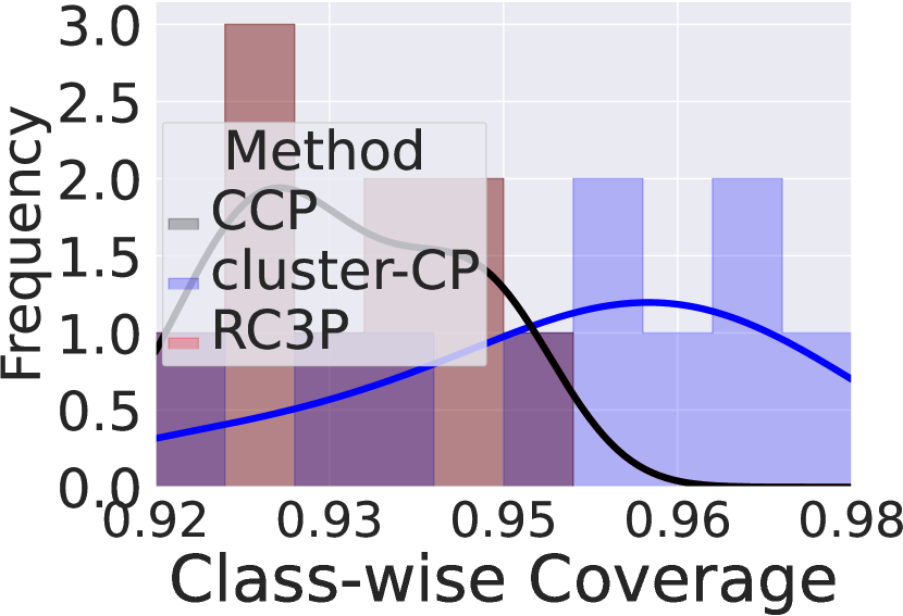
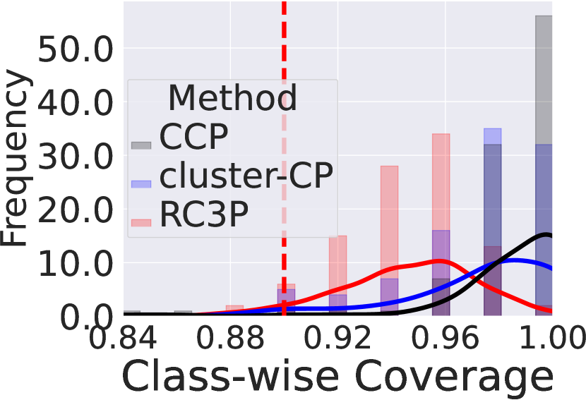
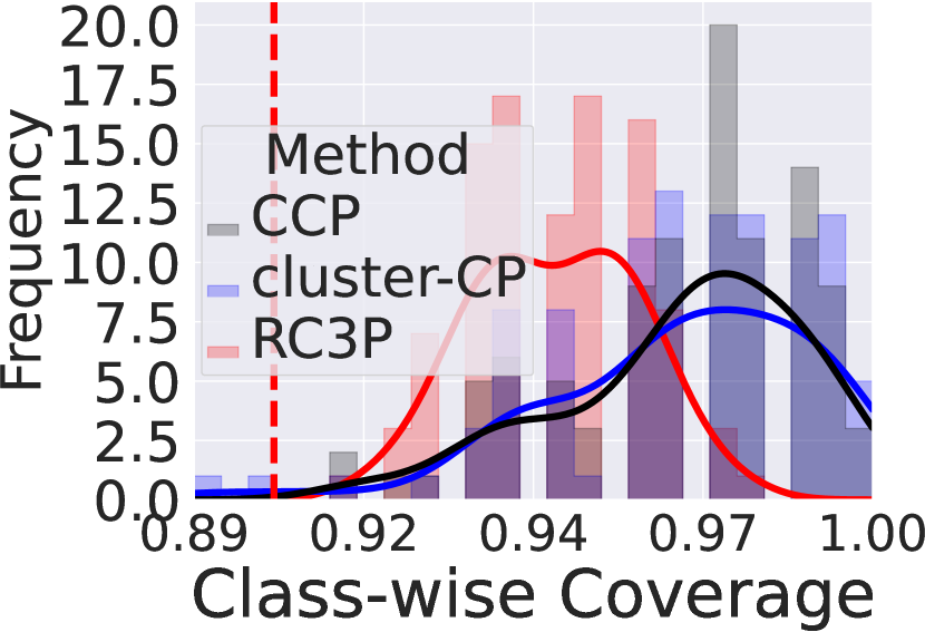
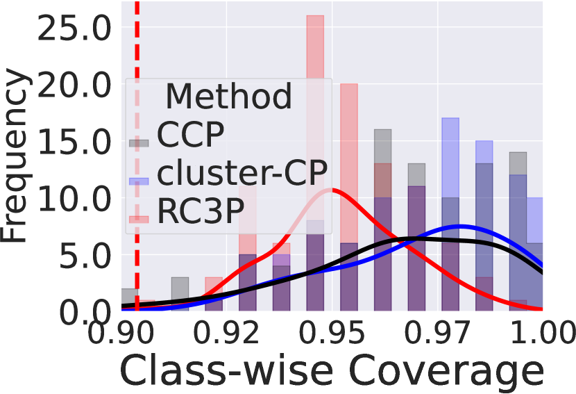
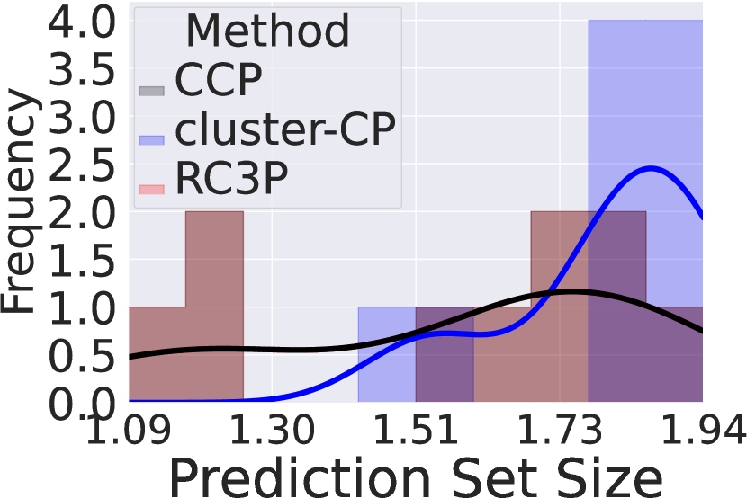
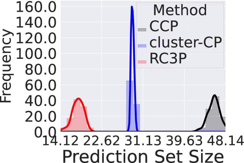
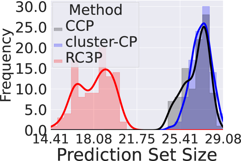
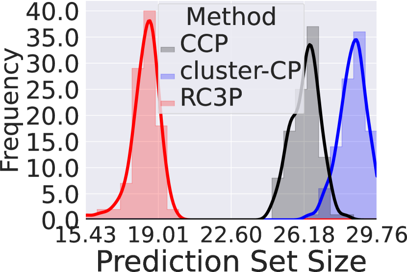
Figure 5: Class-conditional coverage (Top row) and prediction set size (Bottom row) achieved by CCP, Cluster-CP, and RC3P methods when $\alpha=0.1$ on CIFAR-10, CIFAR-100, mini-ImageNet, and Food-101 datasets with imbalance type EXP for imbalance ratio $\rho=0.5$. We clarify that RC3P overlaps with CCP on CIFAR-10. It is clear that RC3P has more densely distributed class-conditional coverage above $0.9$ (the target $1-\alpha$ class-conditional coverage) than CCP and Cluster-CP with significantly smaller prediction sets on CIFAR-100, mini-ImageNet and Food-101.

(a) CIFAR-10

(b) CIFAR-100

(c) mini-ImageNet

(d) Food-101

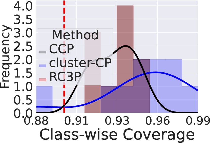
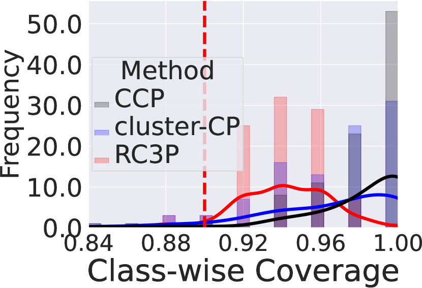
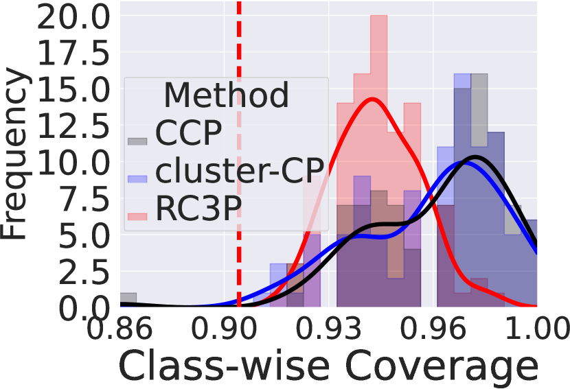
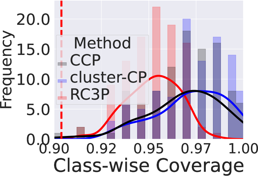
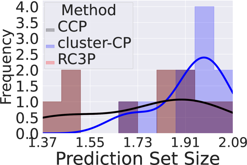
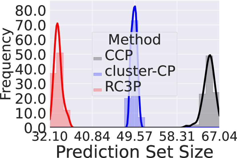
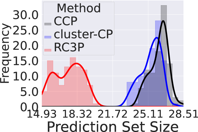
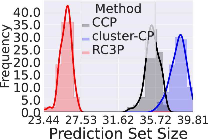
Figure 6: Class-conditional coverage (Top row) and prediction set size (Bottom row) achieved by CCP, Cluster-CP, and RC3P methods when $\alpha=0.1$ on CIFAR-10, CIFAR-100, mini-ImageNet, and Food-101 datasets with imbalance type POLY for imbalance ratio $\rho=0.1$. We clarify that RC3P overlaps with CCP on CIFAR-10. It is clear that RC3P has more densely distributed class-conditional coverage above $0.9$ (the target $1-\alpha$ class-conditional coverage) than CCP and Cluster-CP with significantly smaller prediction sets on CIFAR-100, mini-ImageNet and Food-101.

(a) CIFAR-10

(b) CIFAR-100

(c) mini-ImageNet

(d) Food-101

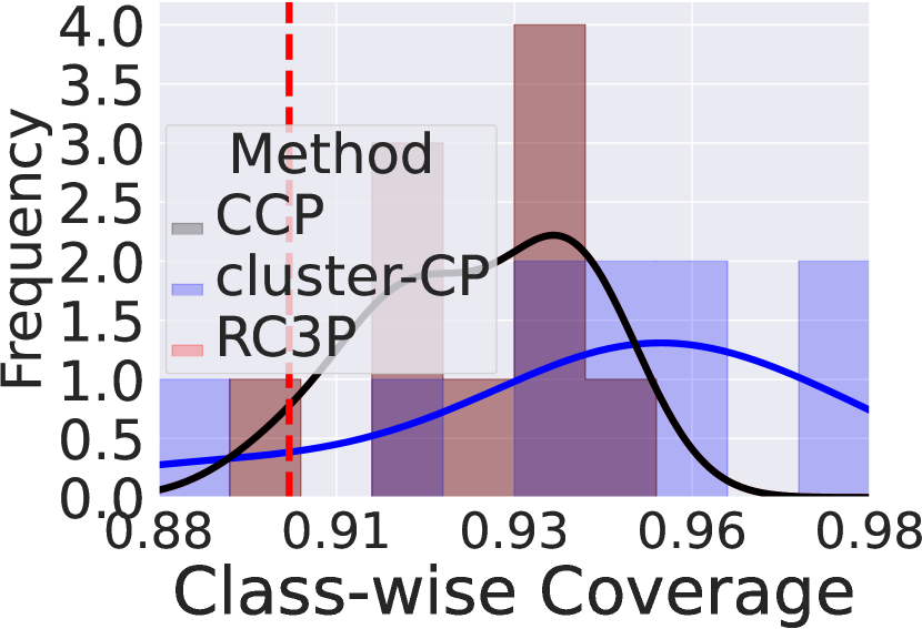
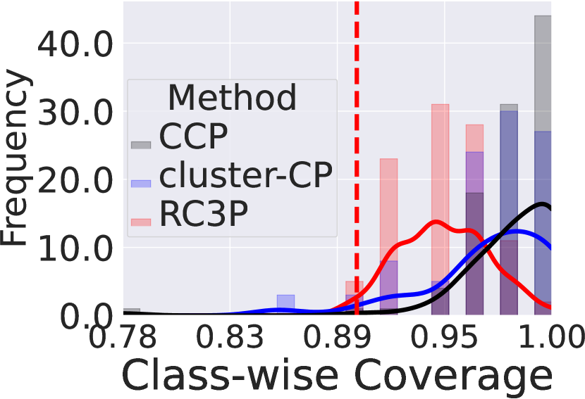
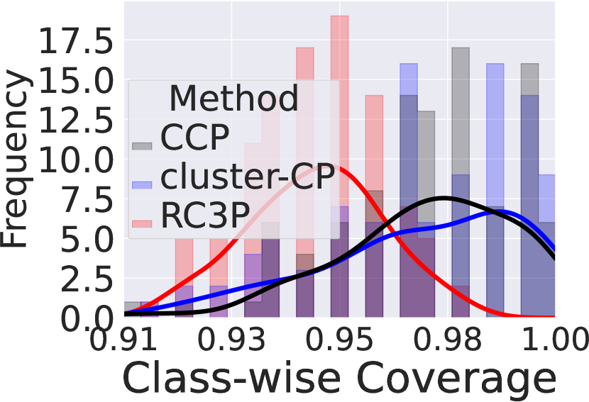
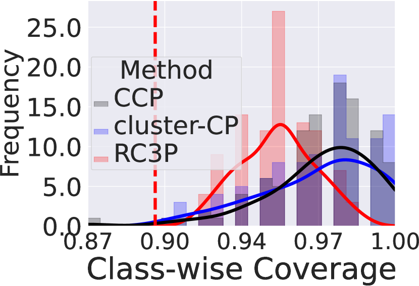
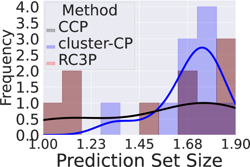
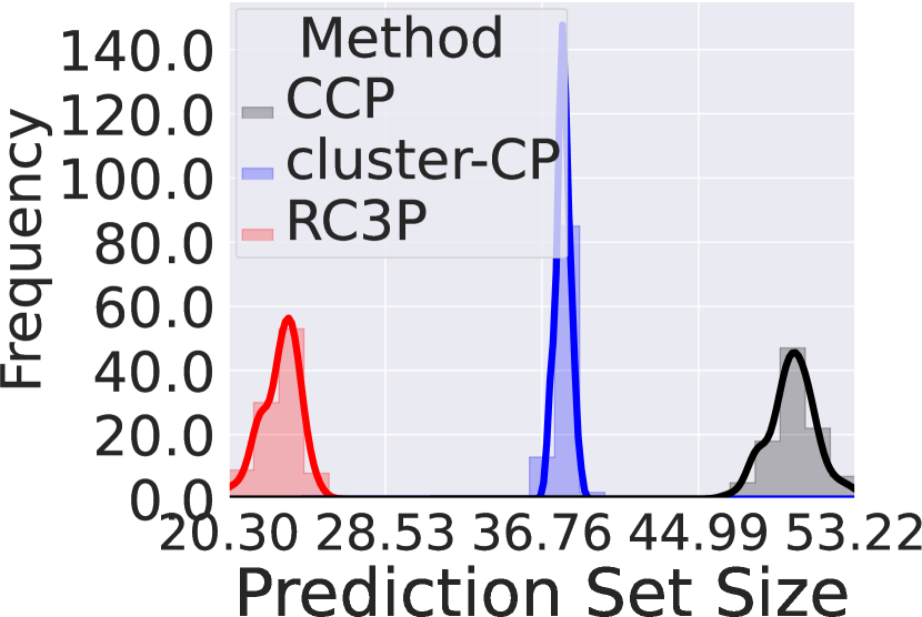
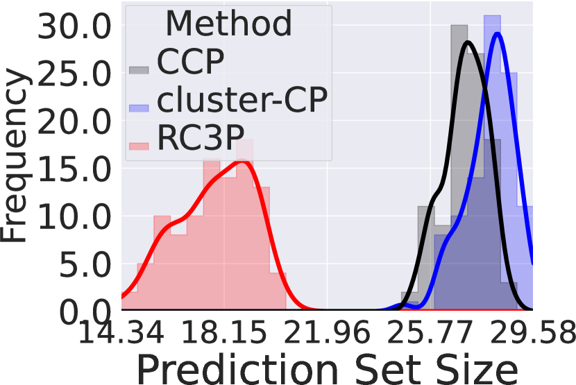
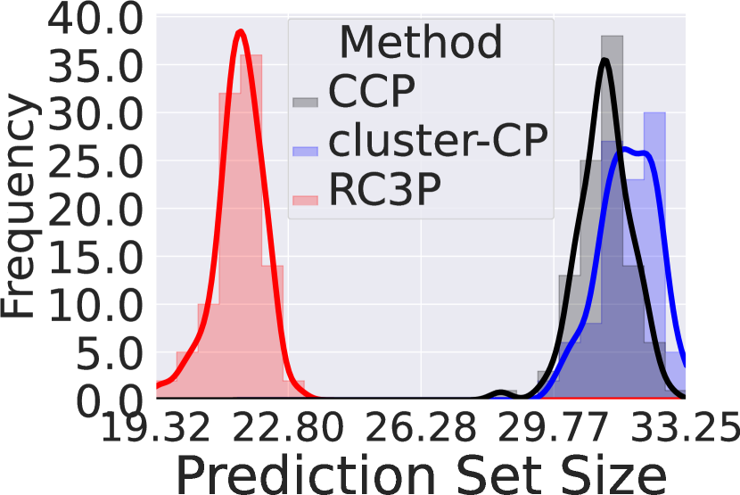
Figure 7: Class-conditional coverage (Top row) and prediction set size (Bottom row) achieved by CCP, Cluster-CP, and RC3P methods when $\alpha=0.1$ on CIFAR-10, CIFAR-100, mini-ImageNet, and Food-101 datasets with imbalance type POLY for imbalance ratio $\rho=0.5$. We clarify that RC3P overlaps with CCP on CIFAR-10. It is clear that RC3P has more densely distributed class-conditional coverage above $0.9$ (the target $1-\alpha$ class-conditional coverage) than CCP and Cluster-CP with significantly smaller prediction sets on CIFAR-100, mini-ImageNet and Food-101.

(a) CIFAR-10

(b) CIFAR-100

(c) mini-ImageNet

(d) Food-101

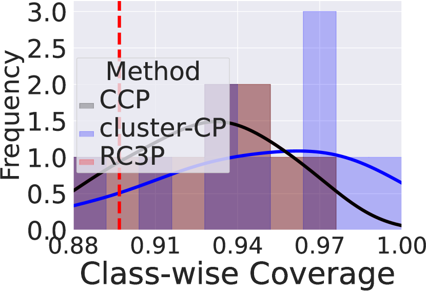
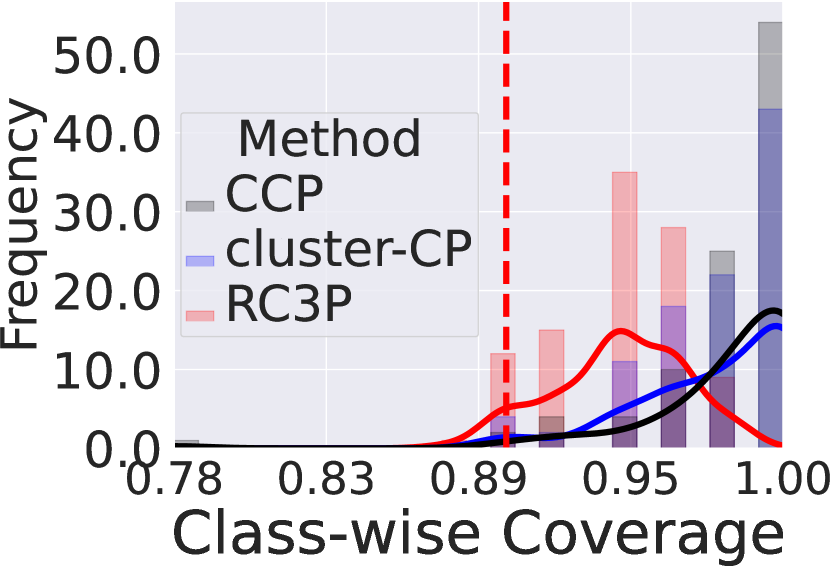
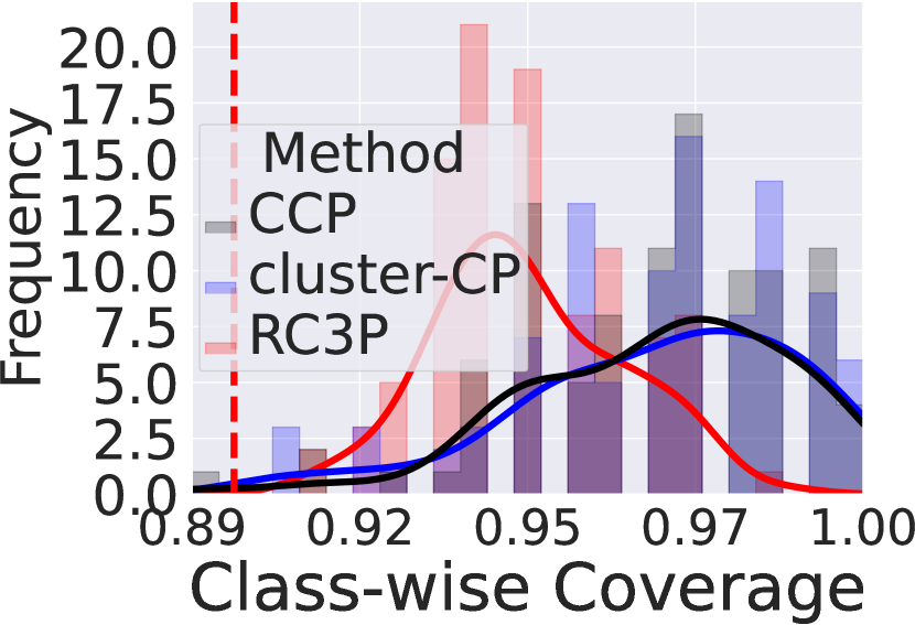
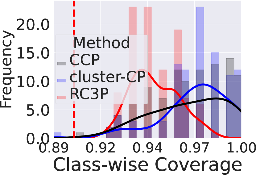
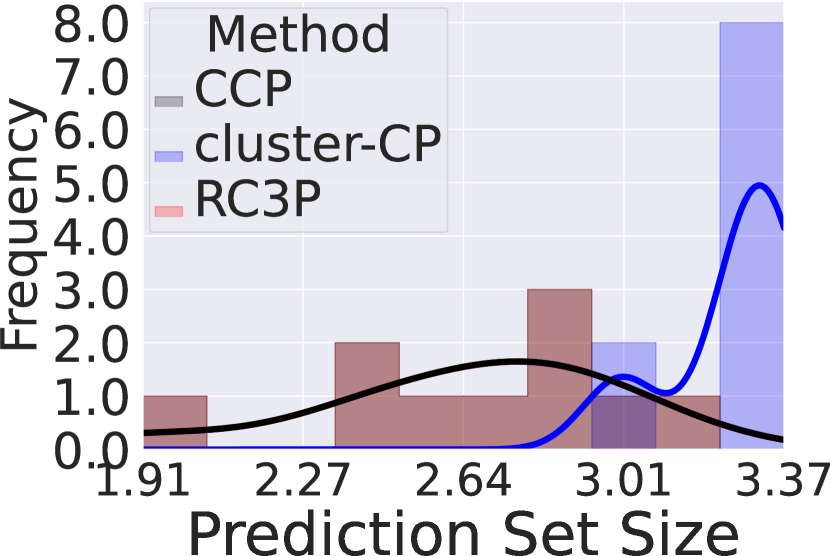
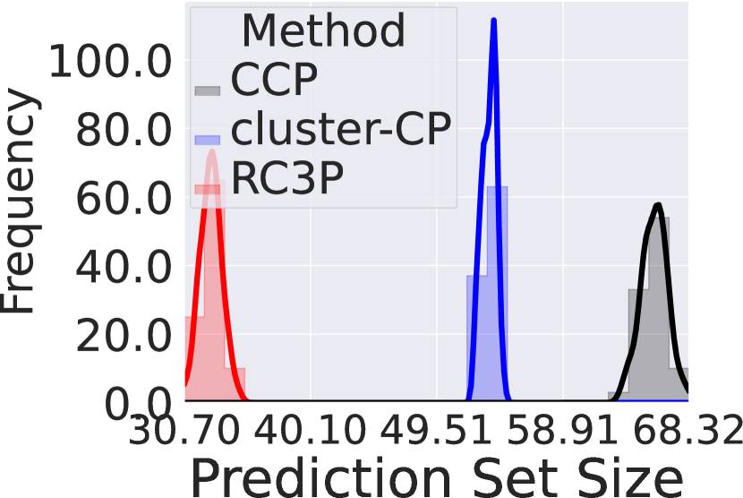
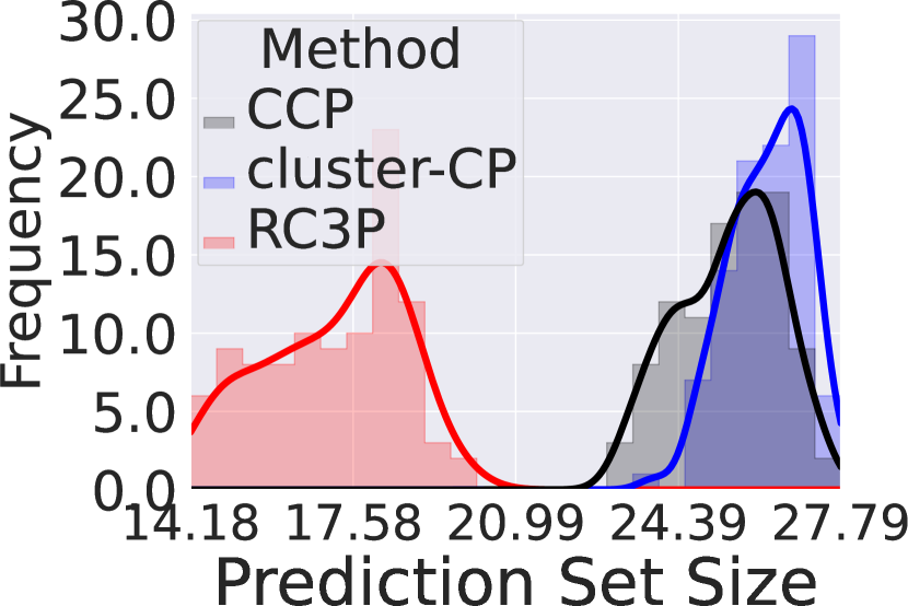
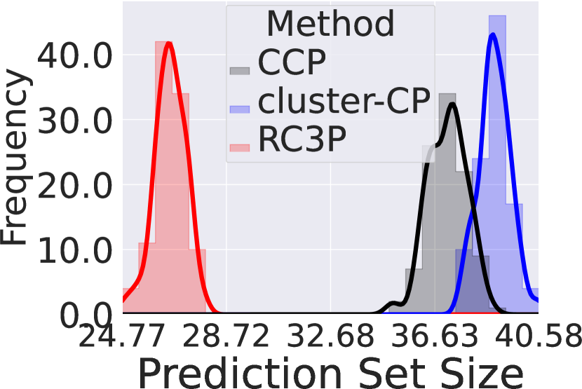
Figure 8: Class-conditional coverage (Top row) and prediction set size (Bottom row) achieved by CCP, Cluster-CP, and RC3P methods when $\alpha=0.1$ on CIFAR-10, CIFAR-100, mini-ImageNet, and Food-101 datasets with imbalance type MAJ for imbalance ratio $\rho=0.1$. We clarify that RC3P overlaps with CCP on CIFAR-10. It is clear that RC3P has more densely distributed class-conditional coverage above $0.9$ (the target $1-\alpha$ class-conditional coverage) than CCP and Cluster-CP with significantly smaller prediction sets on CIFAR-100, mini-ImageNet and Food-101.

(a) CIFAR-10

(b) CIFAR-100

(c) mini-ImageNet

(d) Food-101

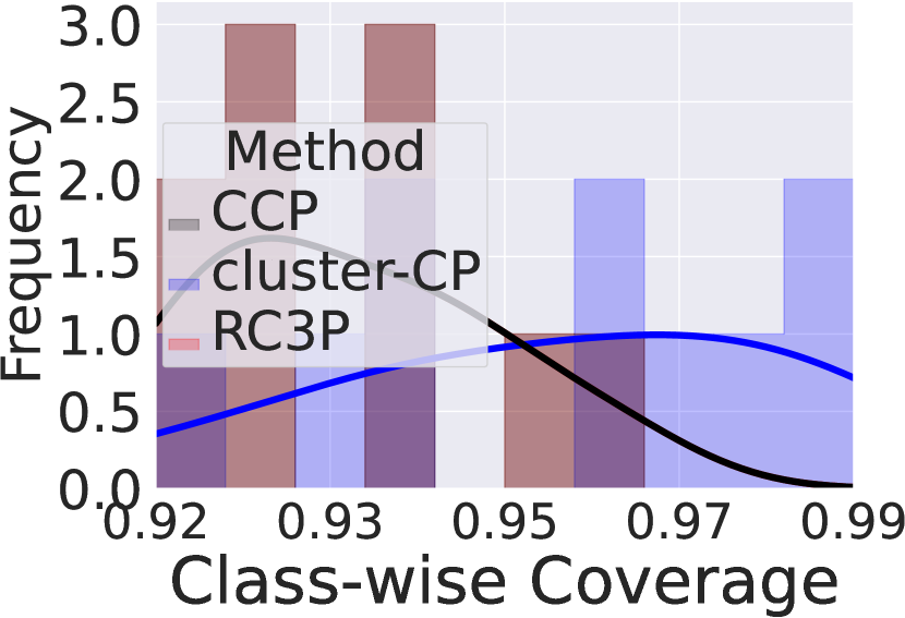
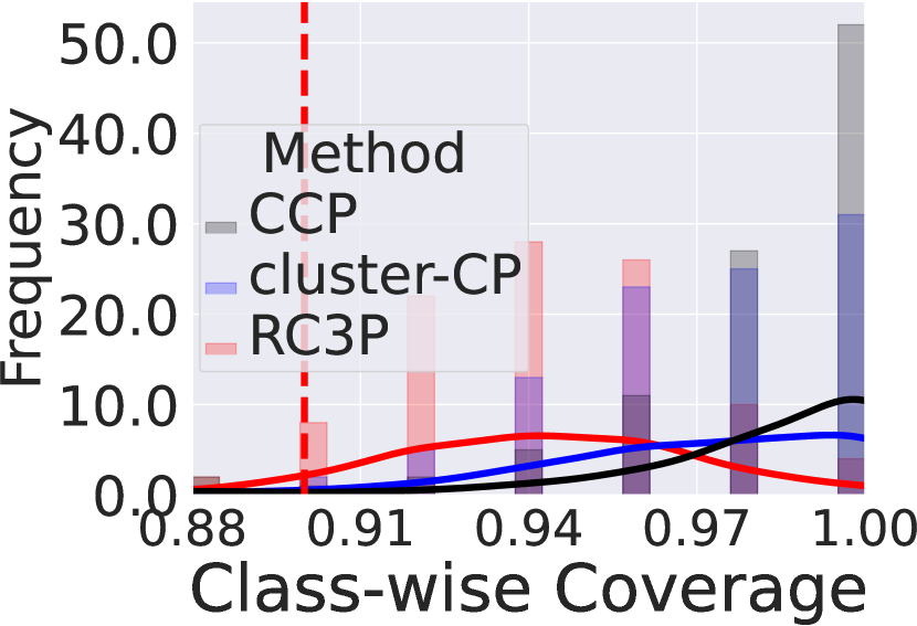
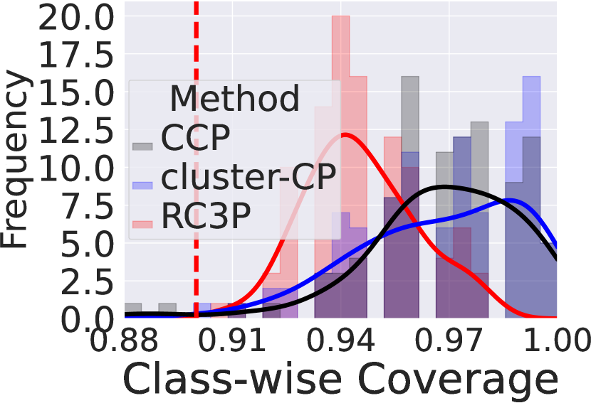
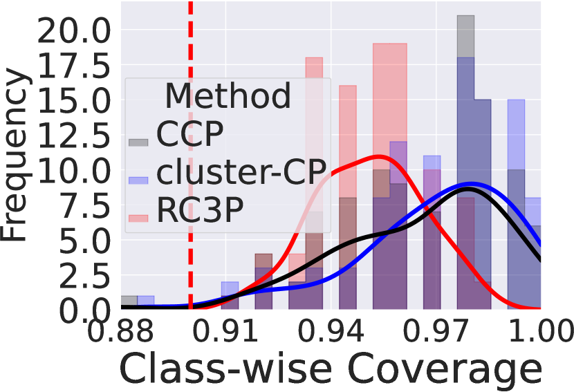
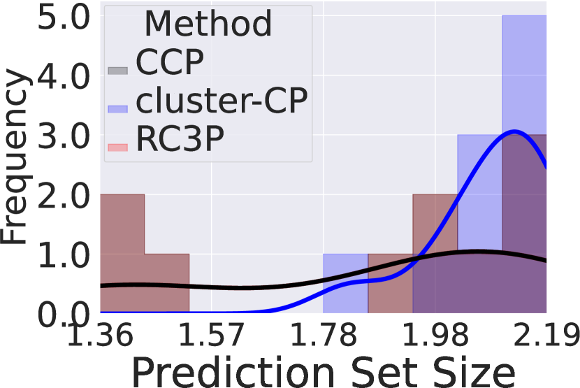
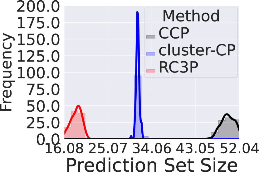
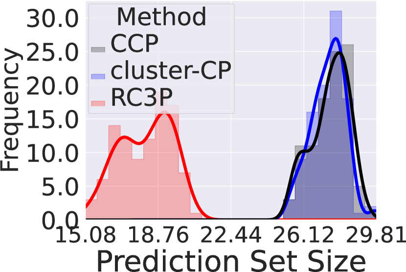
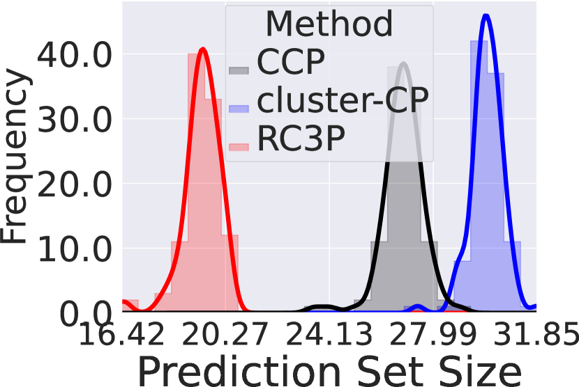
Figure 9: Class-conditional coverage (Top row) and prediction set size (Bottom row) achieved by CCP, Cluster-CP, and RC3P methods when $\alpha=0.1$ on CIFAR-10, CIFAR-100, mini-ImageNet, and Food-101 datasets with imbalance type MAJ for imbalance ratio $\rho=0.5$. We clarify that RC3P overlaps with CCP on CIFAR-10. It is clear that RC3P has more densely distributed class-conditional coverage above $0.9$ (the target $1-\alpha$ class-conditional coverage) than CCP and Cluster-CP with significantly smaller prediction sets on CIFAR-100, mini-ImageNet and Food-101.

(a) CIFAR-10

(b) CIFAR-100

(c) mini-ImageNet

(d) Food-101

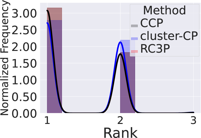
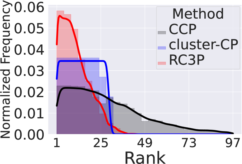
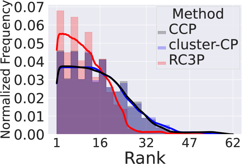
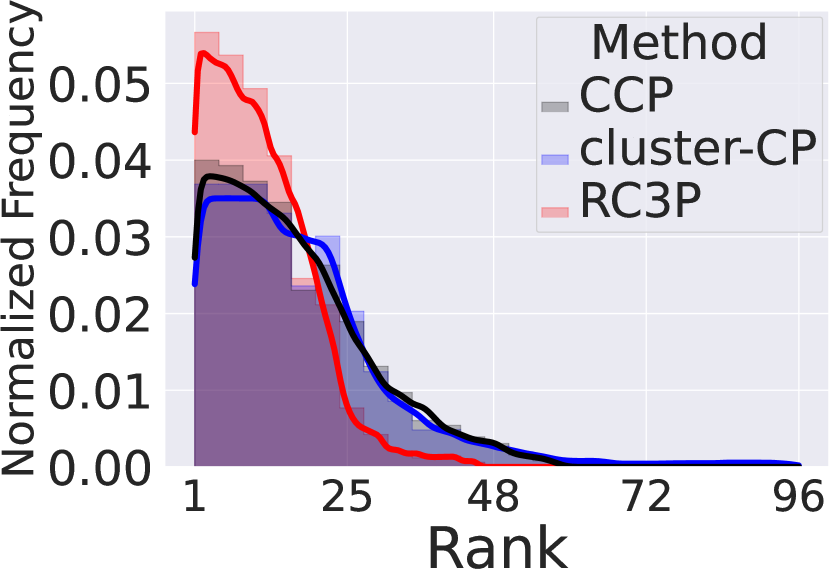
Figure 10: Visualization for the normalized frequency distribution of label ranks included in the prediction set of CCP, Cluster-CP, and RC3P with $\rho=0.5$ EXP when $\alpha=0.1$. It is clear that the distribution of normalized frequency generated by RC3P tends to be lower compared to those produced by CCP and Cluster-CP. Furthermore, the probability density function tail for label ranks in the RC3P prediction set is notably shorter than that of other methods.

(a) CIFAR-10

(b) CIFAR-100

(c) mini-ImageNet

(d) Food-101

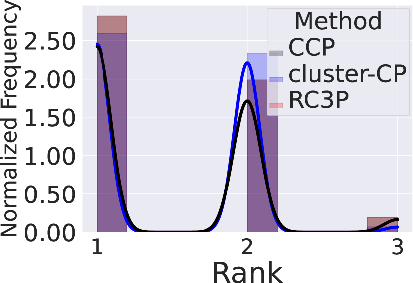
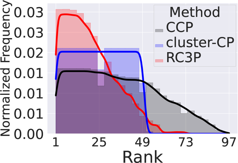
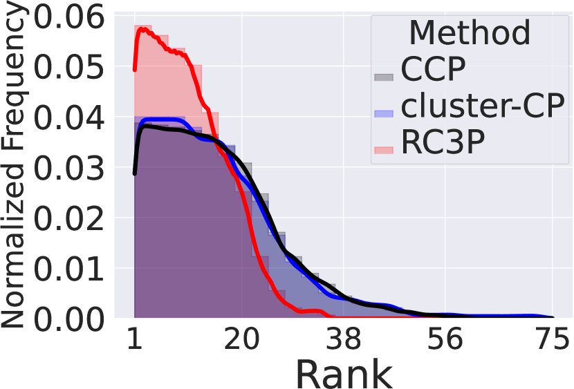
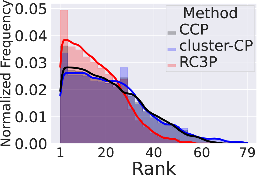
Figure 11: Visualization for the normalized frequency distribution of label ranks included in the prediction set of CCP, Cluster-CP, and RC3P with $\rho=0.1$ POLY when $\alpha=0.1$. It is clear that the distribution of normalized frequency generated by RC3P tends to be lower compared to those produced by CCP and Cluster-CP. Furthermore, the probability density function tail for label ranks in the RC3P prediction set is notably shorter than that of other methods.

(a) CIFAR-10

(b) CIFAR-100

(c) mini-ImageNet

(d) Food-101

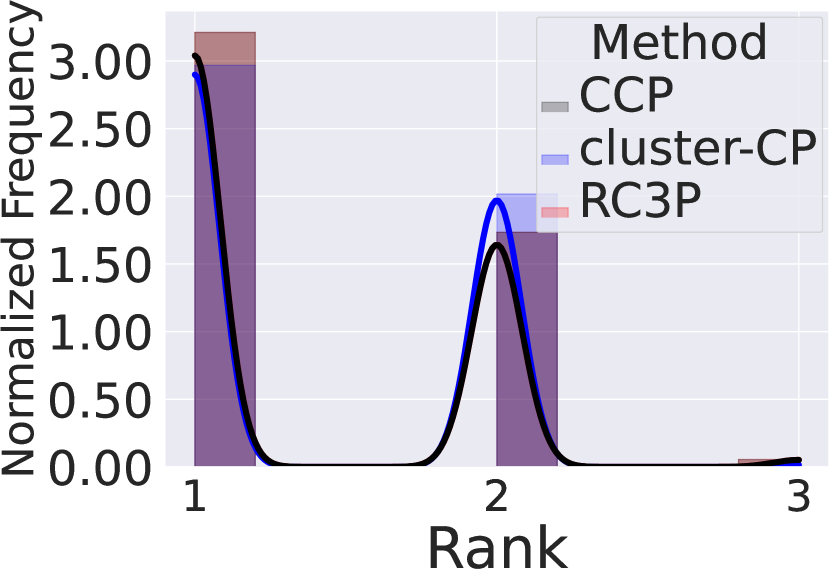
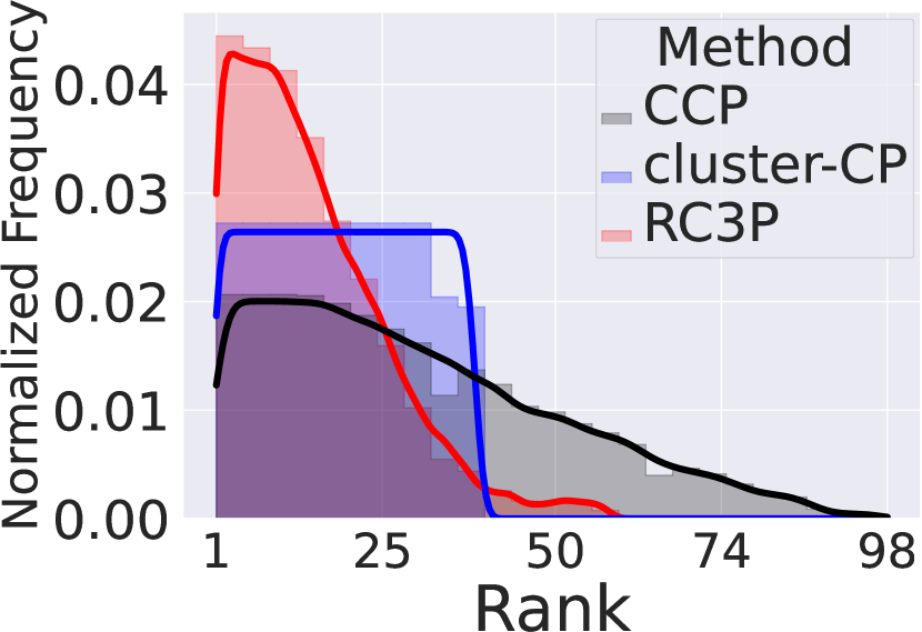
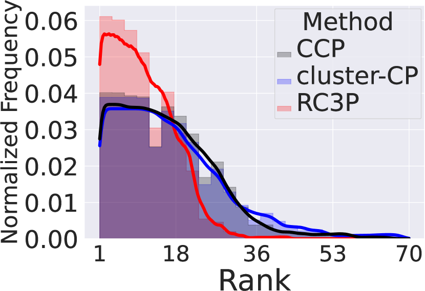
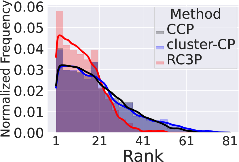
Figure 12: Visualization for the normalized frequency distribution of label ranks included in the prediction set of CCP, Cluster-CP, and RC3P with $\rho=0.5$ POLY when $\alpha=0.1$. It is clear that the distribution of normalized frequency generated by RC3P tends to be lower compared to those produced by CCP and Cluster-CP. Furthermore, the probability density function tail for label ranks in the RC3P prediction set is notably shorter than that of other methods.

(a) CIFAR-10

(b) CIFAR-100

(c) mini-ImageNet

(d) Food-101

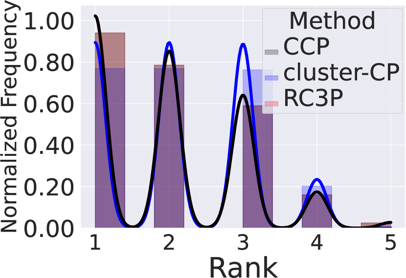
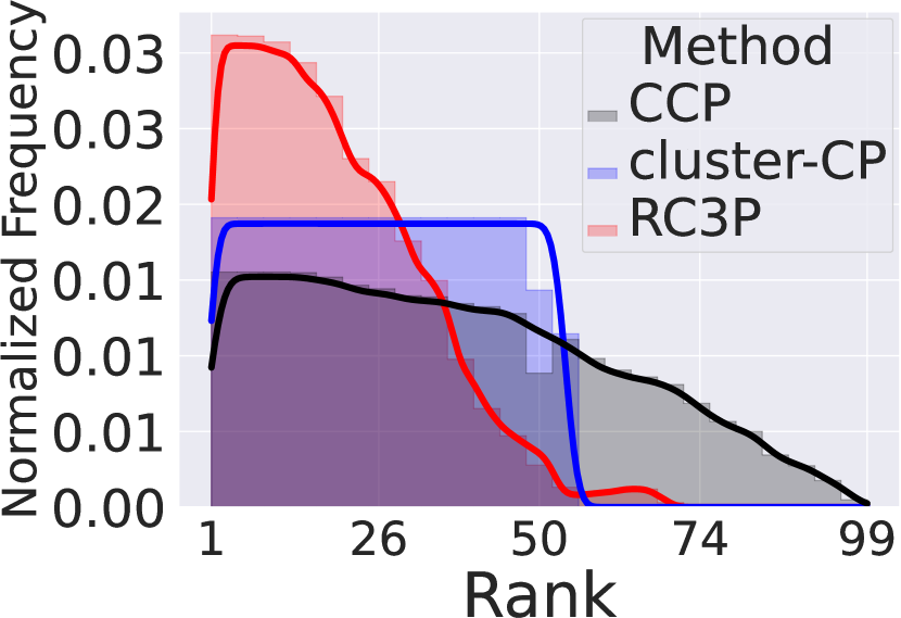
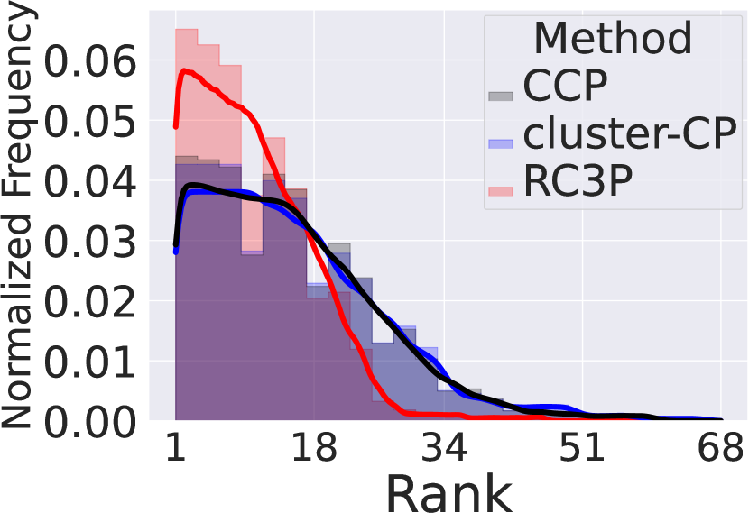
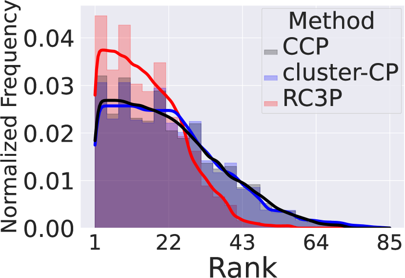
Figure 13: Visualization for the normalized frequency distribution of label ranks included in the prediction set of CCP, Cluster-CP, and RC3P with $\rho=0.1$ MAJ when $\alpha=0.1$. It is clear that the distribution of normalized frequency generated by RC3P tends to be lower compared to those produced by CCP and Cluster-CP. Furthermore, the probability density function tail for label ranks in the RC3P prediction set is notably shorter than that of other methods.

(a) CIFAR-10

(b) CIFAR-100

(c) mini-ImageNet

(d) Food-101

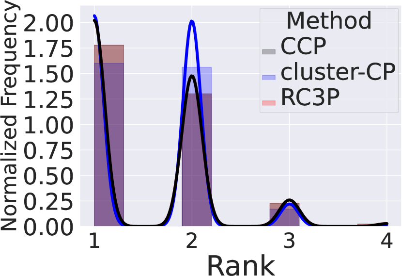
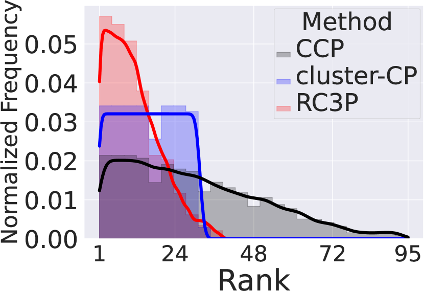
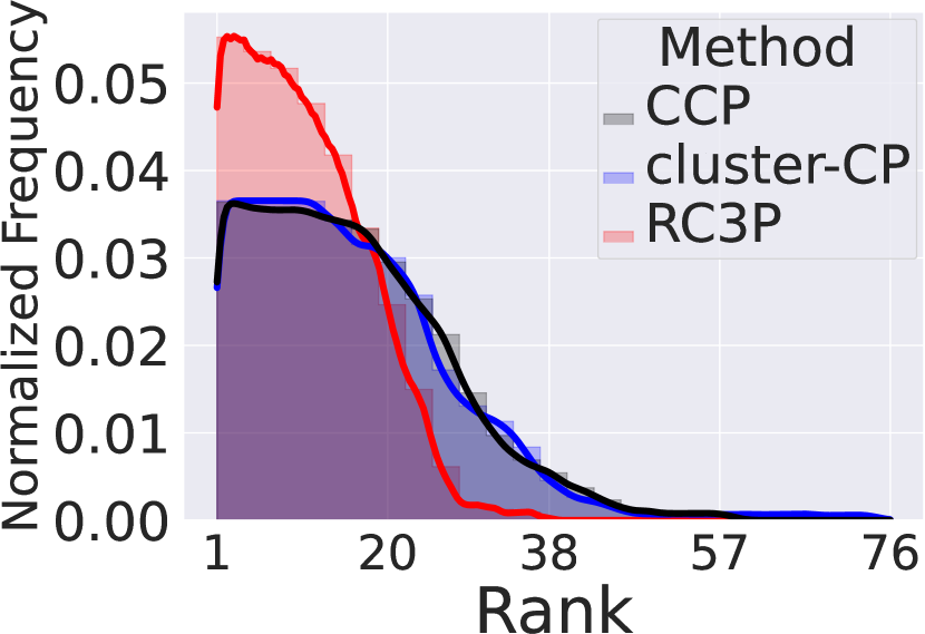
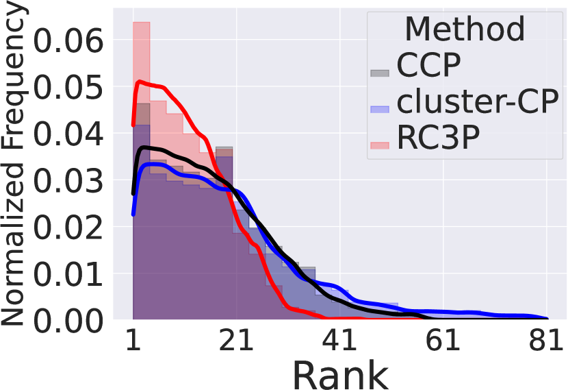
Figure 14: Visualization for the normalized frequency distribution of label ranks included in the prediction set of CCP, Cluster-CP, and RC3P with $\rho=0.5$ MAJ when $\alpha=0.1$. It is clear that the distribution of normalized frequency generated by RC3P tends to be lower compared to those produced by CCP and Cluster-CP. Furthermore, the probability density function tail for label ranks in the RC3P prediction set is notably shorter than that of other methods.

(a) CIFAR-10

(b) CIFAR-100

(c) mini-ImageNet

(d) Food-101

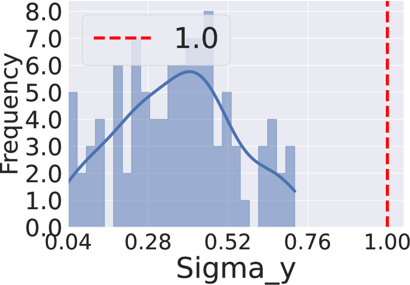
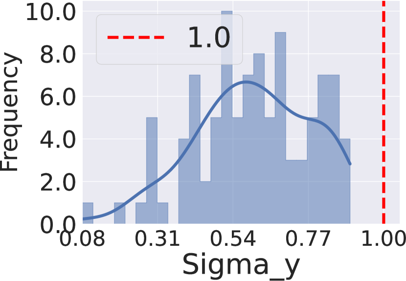
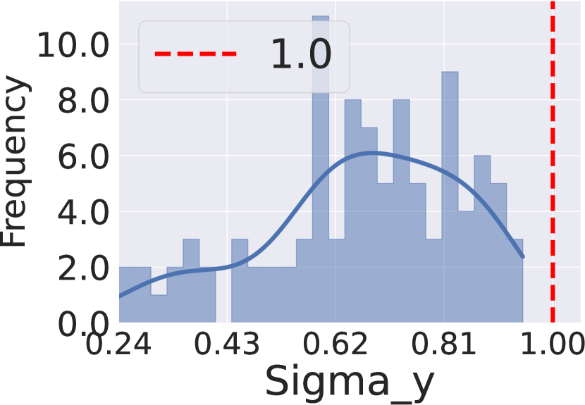
Figure 15: Verification of condition numbers $\{\sigma_{y}\}_{y=1}^{C}$ of Equation 6 when epoch $=200$ and $\alpha=0.1$ with $\rho=0.5$ EXP. Vertical dashed lines represent the value $1$, and we observe that all the condition numbers are smaller than $1$. This verifies the validity of the condition for Lemma 4.2, and thus confirms that RC3Pproduces smaller prediction sets than CCP by the optimized trade-off between calibration on non-conformity scores and calibrated label ranks.

(a) CIFAR-10

(b) CIFAR-100

(c) mini-ImageNet

(d) Food-101

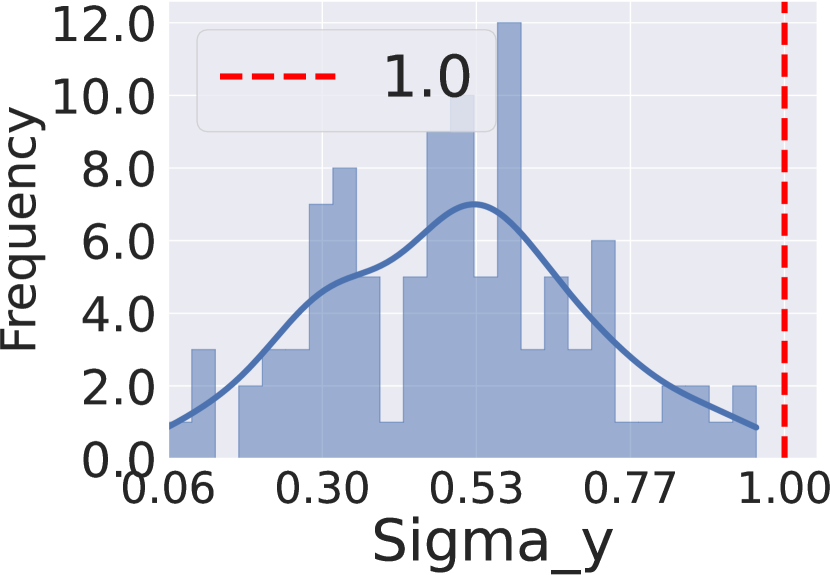
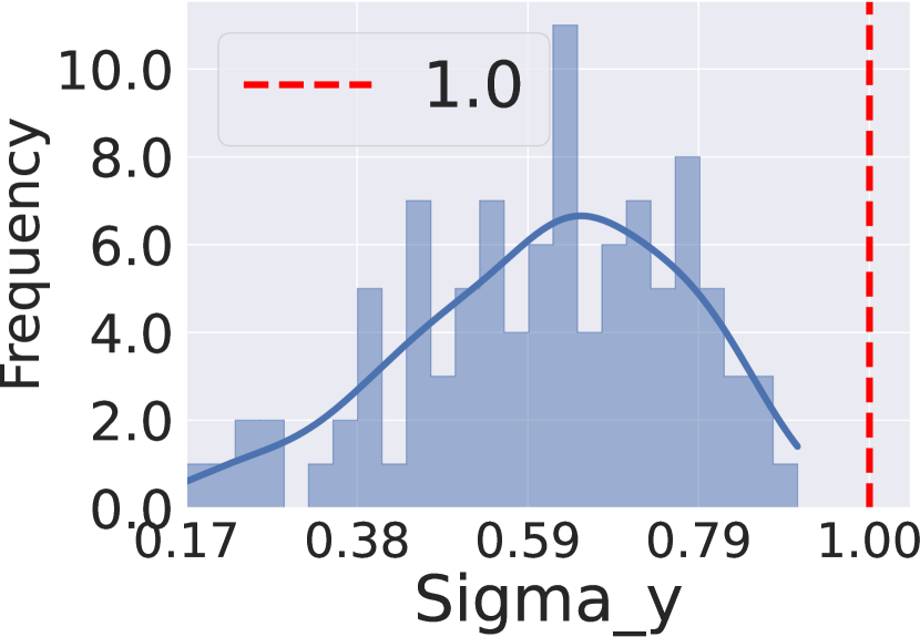
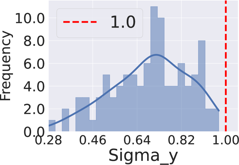
Figure 16: Verification of condition numbers $\{\sigma_{y}\}_{y=1}^{C}$ of Equation 6 when epoch $=200$ and $\alpha=0.1$ with $\rho=0.1$ POLY. Vertical dashed lines represent the value $1$, and we observe that all the condition numbers are smaller than $1$. This verifies the validity of the condition for Lemma 4.2, and thus confirms that RC3Pproduces smaller prediction sets than CCP by the optimized trade-off between calibration on non-conformity scores and calibrated label ranks.

(a) CIFAR-10

(b) CIFAR-100

(c) mini-ImageNet

(d) Food-101

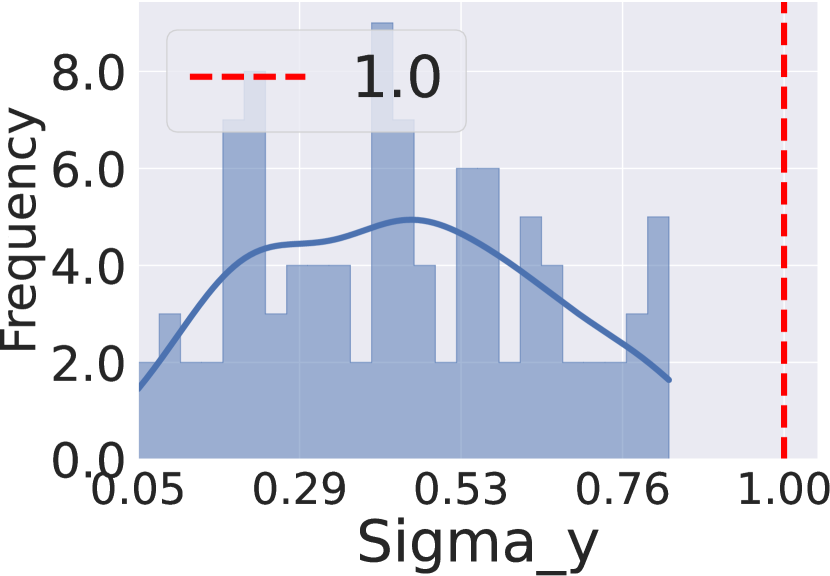
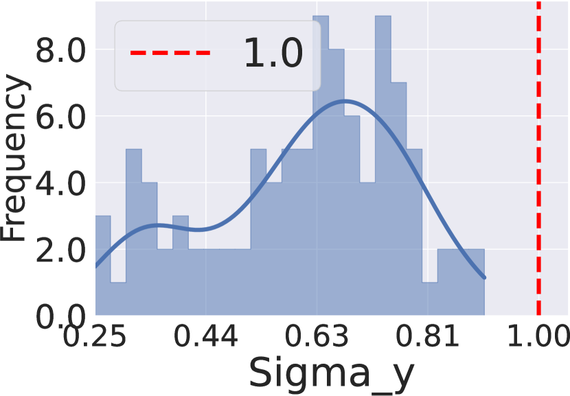
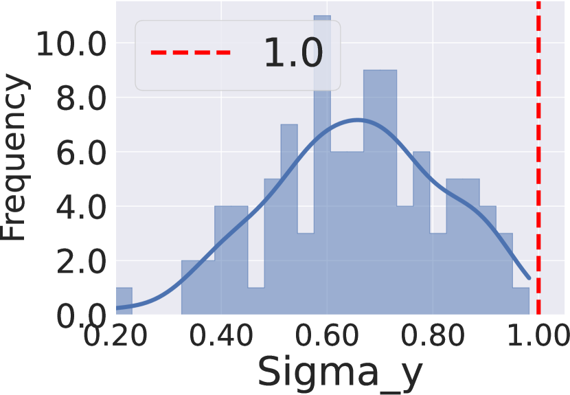
Figure 17: Verification of condition numbers $\{\sigma_{y}\}_{y=1}^{C}$ of Equation 6 when epoch $=200$ and $\alpha=0.1$ with $\rho=0.5$ POLY. Vertical dashed lines represent the value $1$, and we observe that all the condition numbers are smaller than $1$. This verifies the validity of the condition for Lemma 4.2, and thus confirms that RC3Pproduces smaller prediction sets than CCP by the optimized trade-off between calibration on non-conformity scores and calibrated label ranks.

(a) CIFAR-10

(b) CIFAR-100

(c) mini-ImageNet

(d) Food-101

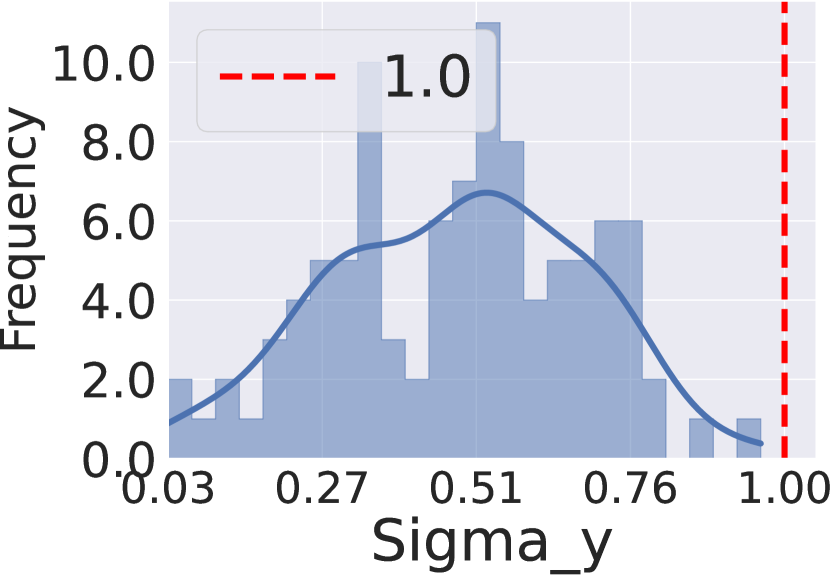
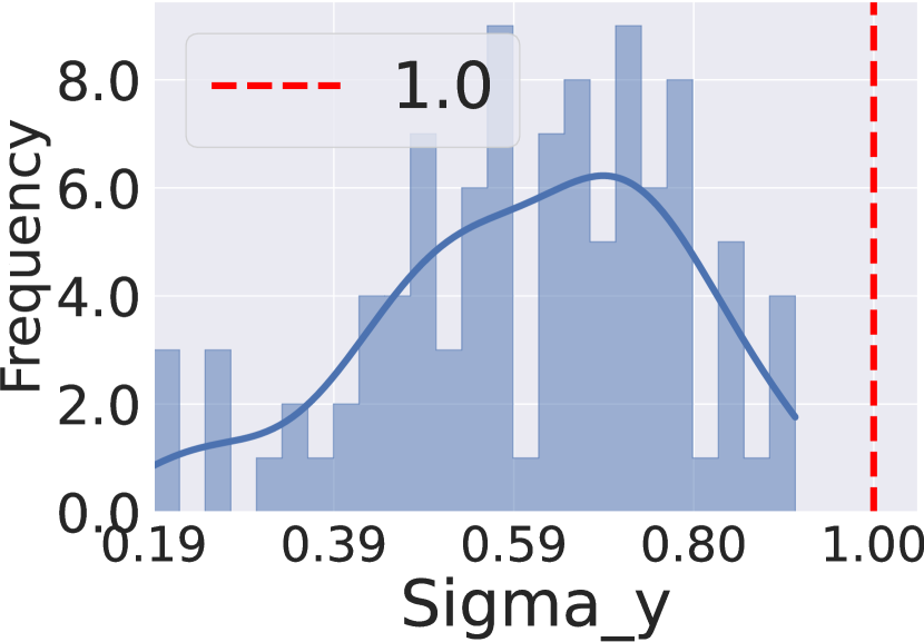
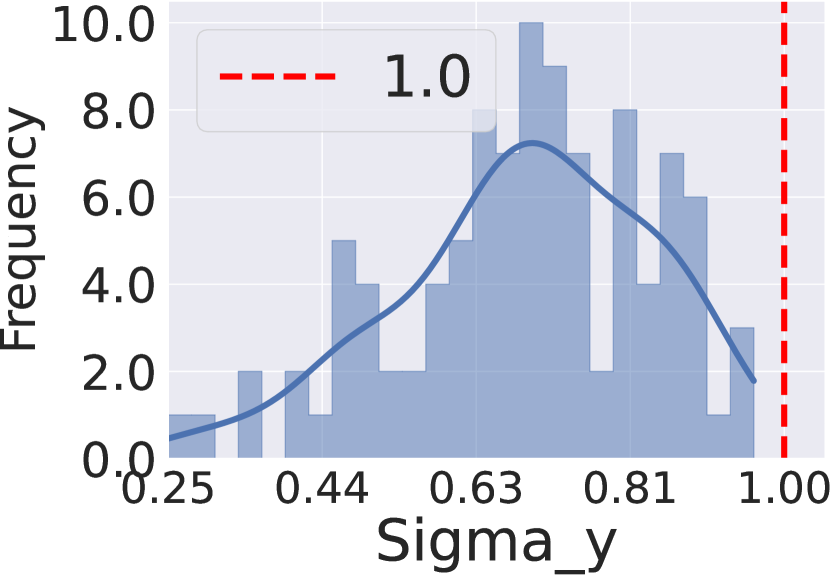
Figure 18: Verification of condition numbers $\{\sigma_{y}\}_{y=1}^{C}$ of Equation 6 when epoch $=200$ and $\alpha=0.1$ with $\rho=0.1$ MAJ. Vertical dashed lines represent the value $1$, and we observe that all the condition numbers are smaller than $1$. This verifies the validity of the condition for Lemma 4.2, and thus confirms that RC3Pproduces smaller prediction sets than CCP by the optimized trade-off between calibration on non-conformity scores and calibrated label ranks.

(a) CIFAR-10

(b) CIFAR-100

(c) mini-ImageNet

(d) Food-101

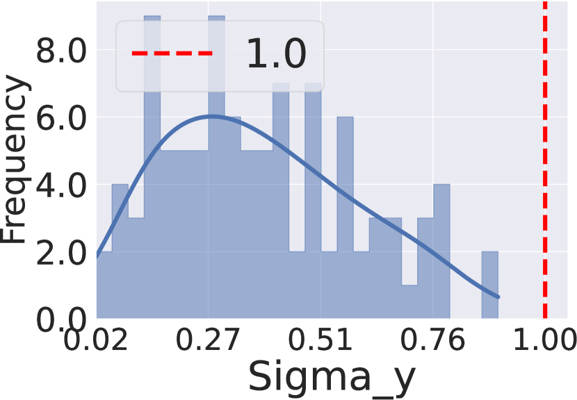
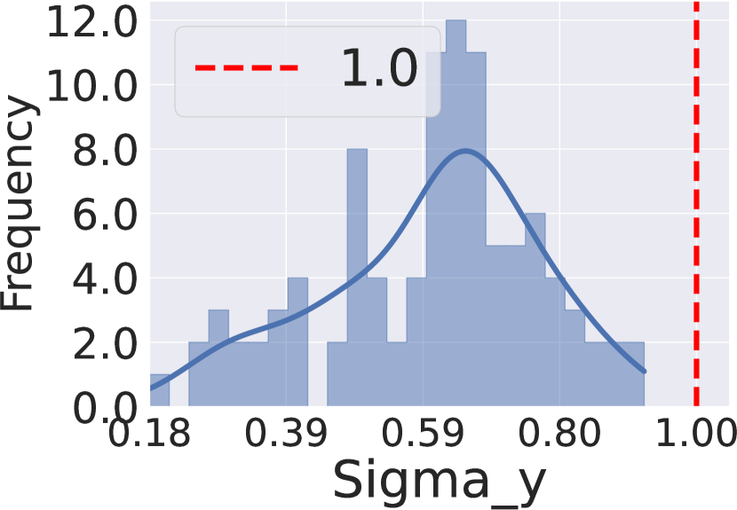
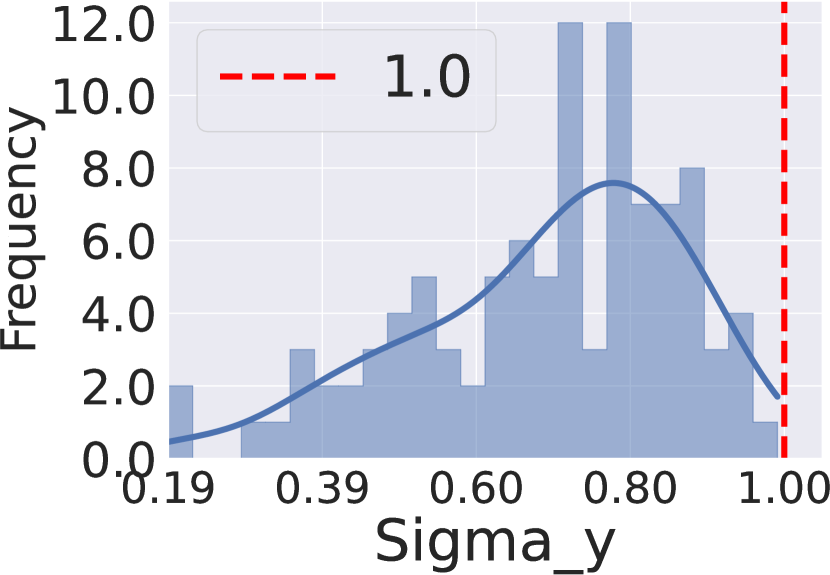
Figure 19: Verification of condition numbers $\{\sigma_{y}\}_{y=1}^{C}$ of Equation 6 when epoch $=200$ and $\alpha=0.1$ with $\rho=0.5$ MAJ. Vertical dashed lines represent the value $1$, and we observe that all the condition numbers are smaller than $1$. This verifies the validity of the condition for Lemma 4.2, and thus confirms that RC3Pproduces smaller prediction sets than CCP by the optimized trade-off between calibration on non-conformity scores and calibrated label ranks.

(a) CIFAR-10

(b) CIFAR-100

(c) mini-ImageNet

(d) Food-101

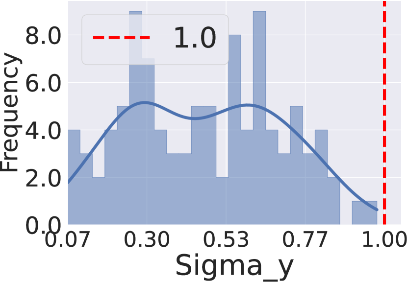
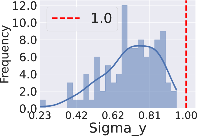
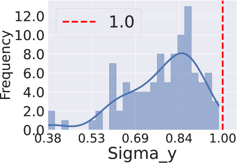
Figure 20: Verification of condition numbers $\{\sigma_{y}\}_{y=1}^{C}$ of Equation 6 when epoch $=50$ and $\alpha=0.1$ with $\rho=0.1$ EXP. Vertical dashed lines represent the value $1$, and we observe that all the condition numbers are smaller than $1$. This verifies the validity of the condition for Lemma 4.2, and thus confirms that RC3Pproduces smaller prediction sets than CCP by the optimized trade-off between calibration on non-conformity scores and calibrated label ranks.

(a) CIFAR-10

(b) CIFAR-100

(c) mini-ImageNet

(d) Food-101

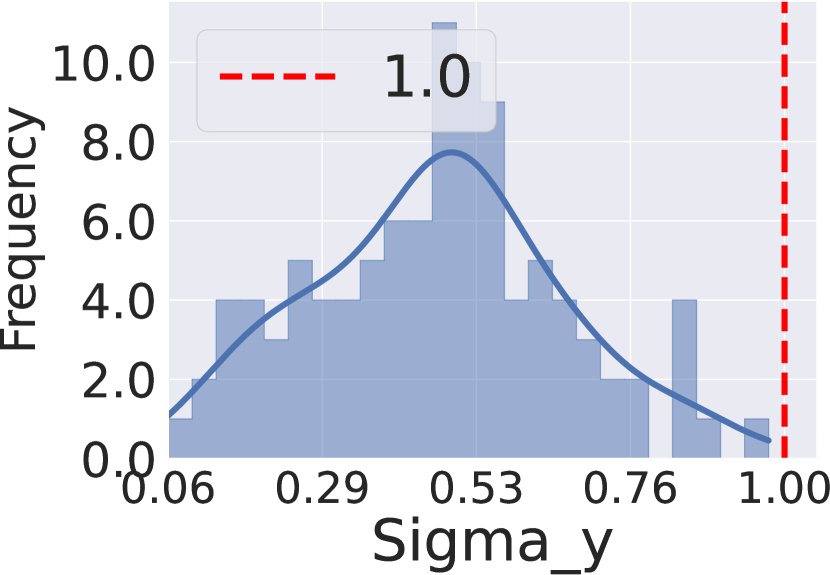
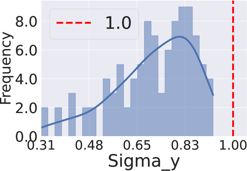
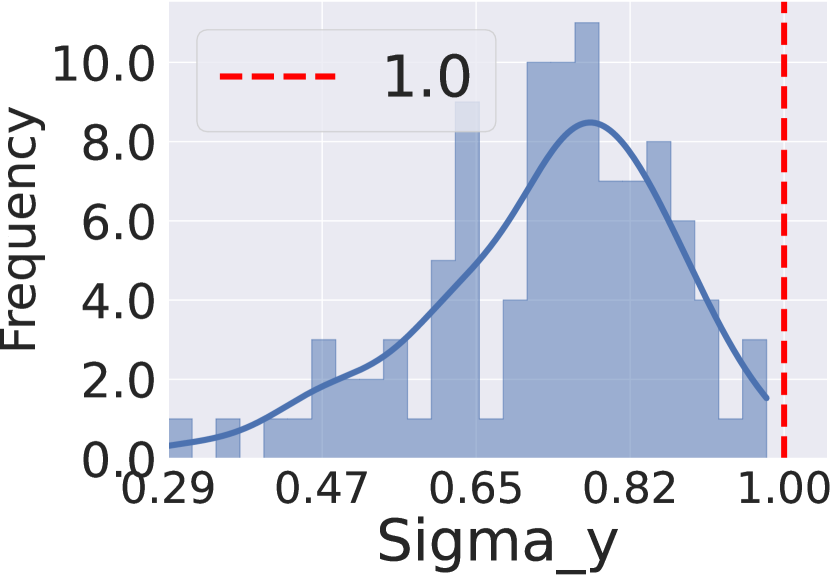
Figure 21: Verification of condition numbers $\{\sigma_{y}\}_{y=1}^{C}$ of Equation 6 when epoch $=50$ and $\alpha=0.1$ with $\rho=0.5$ EXP. Vertical dashed lines represent the value $1$, and we observe that all the condition numbers are smaller than $1$. This verifies the validity of the condition for Lemma 4.2, and thus confirms that RC3Pproduces smaller prediction sets than CCP by the optimized trade-off between calibration on non-conformity scores and calibrated label ranks.

(a) CIFAR-10

(b) CIFAR-100

(c) mini-ImageNet

(d) Food-101

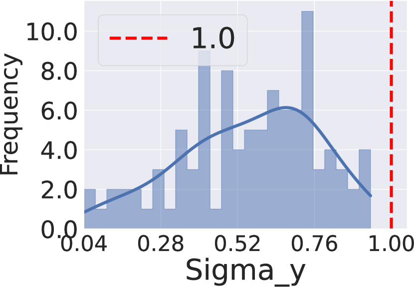
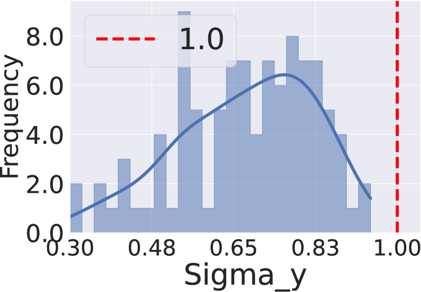
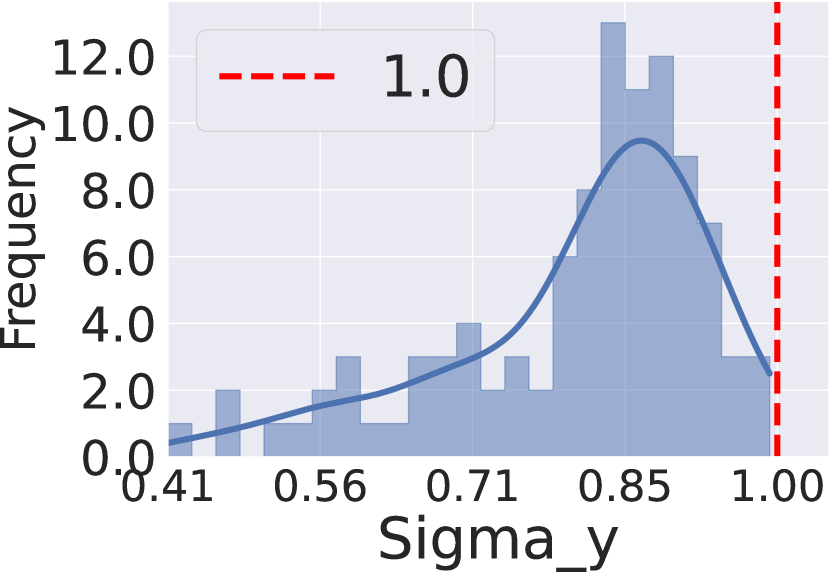
Figure 22: Verification of condition numbers $\{\sigma_{y}\}_{y=1}^{C}$ of Equation 6 when epoch $=50$ and $\alpha=0.1$ with $\rho=0.1$ POLY. Vertical dashed lines represent the value $1$, and we observe that all the condition numbers are smaller than $1$. This verifies the validity of the condition for Lemma 4.2, and thus confirms that RC3Pproduces smaller prediction sets than CCP by the optimized trade-off between calibration on non-conformity scores and calibrated label ranks.

(a) CIFAR-10

(b) CIFAR-100

(c) mini-ImageNet

(d) Food-101

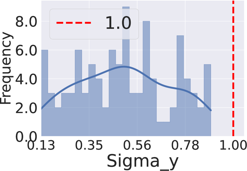
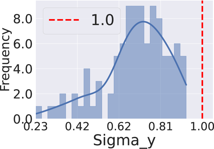
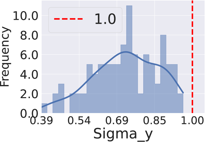
Figure 23: Verification of condition numbers $\{\sigma_{y}\}_{y=1}^{C}$ of Equation 6 when epoch $=50$ and $\alpha=0.1$ with $\rho=0.5$ POLY. Vertical dashed lines represent the value $1$, and we observe that all the condition numbers are smaller than $1$. This verifies the validity of the condition for Lemma 4.2, and thus confirms that RC3Pproduces smaller prediction sets than CCP by the optimized trade-off between calibration on non-conformity scores and calibrated label ranks.

(a) CIFAR-10

(b) CIFAR-100

(c) mini-ImageNet

(d) Food-101

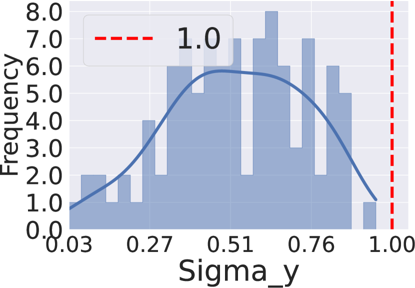
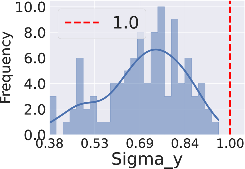
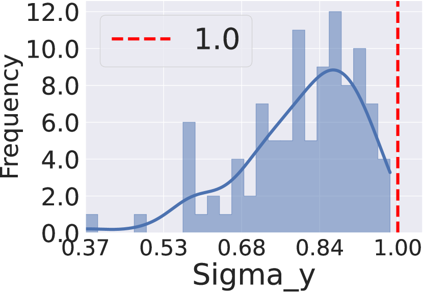
Figure 24: Verification of condition numbers $\{\sigma_{y}\}_{y=1}^{C}$ of Equation 6 when epoch $=50$ and $\alpha=0.1$ with $\rho=0.1$ MAJ. Vertical dashed lines represent the value $1$, and we observe that all the condition numbers are smaller than $1$. This verifies the validity of the condition for Lemma 4.2, and thus confirms that RC3Pproduces smaller prediction sets than CCP by the optimized trade-off between calibration on non-conformity scores and calibrated label ranks.

(a) CIFAR-10

(b) CIFAR-100

(c) mini-ImageNet

(d) Food-101

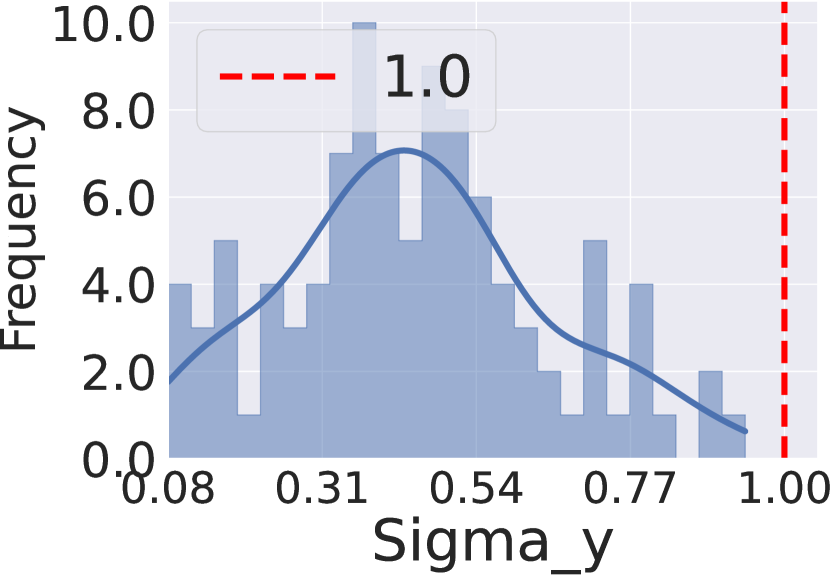
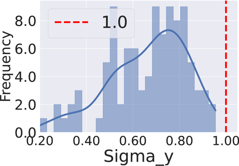
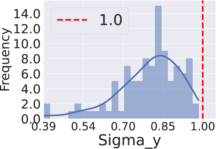
Figure 25: Verification of condition numbers $\{\sigma_{y}\}_{y=1}^{C}$ of Equation 6 when epoch $=50$ and $\alpha=0.1$ with $\rho=0.5$ MAJ. Vertical dashed lines represent the value $1$, and we observe that all the condition numbers are smaller than $1$. This verifies the validity of the condition for Lemma 4.2, and thus confirms that RC3Pproduces smaller prediction sets than CCP by the optimized trade-off between calibration on non-conformity scores and calibrated label ranks.

References

- [1] Ghosh, S., Shi, Y., Belkhouja, T., Yan, Y., Doppa, J. & Jones, B. Probabilistically robust conformal prediction. Uncertainty In Artificial Intelligence. pp. 681-690 (2023)
- [2] Straitouri, E., Wang, L., Okati, N. & Rodriguez, M. Improving Expert Predictions with Conformal Prediction. International Conference On Machine Learning (ICML). (2023)
- [3] Babbar, V., Bhatt, U. & Weller, A. On the utility of prediction sets in human-ai teams. Proceedings Of The Thirty-First International Joint Conference On Artificial Intelligence (IJCAI-22). (2022)
- [4] Cui, Y., Jia, M., Lin, T., Song, Y. & Belongie, S. Class-balanced loss based on effective number of samples. Proceedings Of The IEEE/CVF Conference On Computer Vision And Pattern Recognition. pp. 9268-9277 (2019)
- [5] Cao, K., Wei, C., Gaidon, A., Arechiga, N. & Ma, T. Learning imbalanced datasets with label-distribution-aware margin loss. Advances In Neural Information Processing Systems. 32 (2019)
- [6] Krizhevsky, A., Hinton, G. & Others Learning multiple layers of features from tiny images. (Toronto, ON, Canada,2009)
- [7] Deng, J., Dong, W., Socher, R., Li, L., Li, K. & Fei-Fei, L. Imagenet: A large-scale hierarchical image database. 2009 IEEE Conference On Computer Vision And Pattern Recognition. pp. 248-255 (2009)
- [8] He, K., Zhang, X., Ren, S. & Sun, J. Deep residual learning for image recognition. Proceedings Of The IEEE Conference On Computer Vision And Pattern Recognition. pp. 770-778 (2016)
- [9] Romano, Y., Sesia, M. & Candes, E. Classification with valid and adaptive coverage. Advances In Neural Information Processing Systems. 33 pp. 3581-3591 (2020)
- [10] Menon, A., Jayasumana, S., Rawat, A., Jain, H., Veit, A. & Kumar, S. Long-tail learning via logit adjustment. ArXiv Preprint ArXiv:2007.07314. (2020)
- [11] Vovk, V., Gammerman, A. & Shafer, G. Algorithmic learning in a random world. (Springer,2005)
- [12] Mohri, M., Rostamizadeh, A. & Talwalkar, A. Foundations of machine learning. (MIT press,2018)
- [13] Lei, J., Robins, J. & Wasserman, L. Distribution-free prediction sets. Journal Of The American Statistical Association. 108, 278-287 (2013)
- [14] Vovk, V., Gammerman, A. & Saunders, C. Machine-learning applications of algorithmic randomness. (1999)
- [15] Shafer, G. & Vovk, V. A Tutorial on Conformal Prediction.. Journal Of Machine Learning Research. 9 (2008)
- [16] Gibbs, I. & Candes, E. Adaptive conformal inference under distribution shift. Advances In Neural Information Processing Systems. 34 pp. 1660-1672 (2021)
- [17] Tibshirani, R., Foygel Barber, R., Candes, E. & Ramdas, A. Conformal prediction under covariate shift. Advances In Neural Information Processing Systems. 32 (2019)
- [18] Sadinle, M., Lei, J. & Wasserman, L. Least ambiguous set-valued classifiers with bounded error levels. Journal Of The American Statistical Association. 114, 223-234 (2019)
- [19] Guan, L. Localized Conformal Prediction: A Generalized Inference Framework for Conformal Prediction. ArXiv Preprint ArXiv:2106.08460. (2021)
- [20] Angelopoulos, A., Bates, S., Malik, J. & Jordan, M. Uncertainty sets for image classifiers using conformal prediction. ArXiv Preprint ArXiv:2009.14193. (2020)
- [21] Angelopoulos, A. & Bates, S. A gentle introduction to conformal prediction and distribution-free uncertainty quantification. ArXiv Preprint ArXiv:2107.07511. (2021)
- [22] Chawla, N., Bowyer, K., Hall, L. & Kegelmeyer, W. SMOTE: synthetic minority over-sampling technique. Journal Of Artificial Intelligence Research. 16 pp. 321-357 (2002)
- [23] Tsai, C., Lin, W., Hu, Y. & Yao, G. Under-sampling class imbalanced datasets by combining clustering analysis and instance selection. Information Sciences. 477 pp. 47-54 (2019)
- [24] Mohammed, R., Rawashdeh, J. & Abdullah, M. Machine learning with oversampling and undersampling techniques: overview study and experimental results. 2020 11th International Conference On Information And Communication Systems (ICICS). pp. 243-248 (2020)
- [25] Krawczyk, B., Koziarski, M. & Woźniak, M. Radial-based oversampling for multiclass imbalanced data classification. IEEE Transactions On Neural Networks And Learning Systems. 31, 2818-2831 (2019)
- [26] Vuttipittayamongkol, P. & Elyan, E. Neighbourhood-based undersampling approach for handling imbalanced and overlapped data. Information Sciences. 509 pp. 47-70 (2020)
- [27] Huang, C., Li, Y., Loy, C. & Tang, X. Deep imbalanced learning for face recognition and attribute prediction. IEEE Transactions On Pattern Analysis And Machine Intelligence. 42, 2781-2794 (2019)
- [28] Madabushi, H., Kochkina, E. & Castelle, M. Cost-sensitive BERT for generalisable sentence classification with imbalanced data. ArXiv Preprint ArXiv:2003.11563. (2020)
- [29] Gottlieb, L., Kaufman, E. & Kontorovich, A. Apportioned margin approach for cost sensitive large margin classifiers. Annals Of Mathematics And Artificial Intelligence. 89, 1215-1235 (2021)
- [30] Vovk, V. Conditional validity of inductive conformal predictors. Asian Conference On Machine Learning. pp. 475-490 (2012)
- [31] Vinyals, O., Blundell, C., Lillicrap, T., Wierstra, D. & Others Matching networks for one shot learning. Advances In Neural Information Processing Systems. 29 (2016)
- [32] Bossard, L., Guillaumin, M. & Van Gool, L. Food-101–mining discriminative components with random forests. Computer Vision–ECCV 2014: 13th European Conference, Zurich, Switzerland, September 6-12, 2014, Proceedings, Part VI 13. pp. 446-461 (2014)
- [33] Ding, T., Angelopoulos, A., Bates, S., Jordan, M. & Tibshirani, R. Class-Conditional Conformal Prediction With Many Classes. ArXiv Preprint ArXiv:2306.09335. (2023)
- [34] Romano, Y., Patterson, E. & Candes, E. Conformalized quantile regression. Advances In Neural Information Processing Systems. 32 (2019)
- [35] Huang, J., Xi, H., Zhang, L., Yao, H., Qiu, Y. & Wei, H. Conformal Prediction for Deep Classifier via Label Ranking. ArXiv Preprint ArXiv:2310.06430. (2023)
- [36] Ghosh, S., Belkhouja, T., Yan, Y. & Doppa, J. Improving Uncertainty Quantification of Deep Classifiers via Neighborhood Conformal Prediction: Novel Algorithm and Theoretical Analysis. ArXiv Preprint ArXiv:2303.10694. (2023)
- [37] Boström, H., Johansson, U. & Löfström, T. Mondrian conformal predictive distributions. Conformal And Probabilistic Prediction And Applications. pp. 24-38 (2021)
- [38] Romano, Y., Barber, R., Sabatti, C. & Candès, E. With malice toward none: Assessing uncertainty via equalized coverage. Harvard Data Science Review. 2, 4 (2020)
- [39] Zaffran, M., Dieuleveut, A., Josse, J. & Romano, Y. Conformal prediction with missing values. ArXiv Preprint ArXiv:2306.02732. (2023)
- [40] Fisch, A., Schuster, T., Jaakkola, T. & Barzilay, R. Few-shot conformal prediction with auxiliary tasks. International Conference On Machine Learning. pp. 3329-3339 (2021)
- [41] Lu, C., Lemay, A., Chang, K., Höbel, K. & Kalpathy-Cramer, J. Fair conformal predictors for applications in medical imaging. Proceedings Of The AAAI Conference On Artificial Intelligence. 36, 12008-12016 (2022)
- [42] Fontana, M., Zeni, G. & Vantini, S. Conformal prediction: a unified review of theory and new challenges. Bernoulli. 29, 1-23 (2023)
- [43] Fisch, A., Schuster, T., Jaakkola, T. & Barzilay, R. Efficient conformal prediction via cascaded inference with expanded admission. ArXiv Preprint ArXiv:2007.03114. (2020)
- [44] Vovk, V., Lindsay, D., Nouretdinov, I. & Gammerman, A. Mondrian confidence machine. Technical Report. (2003)
- [45] Lei, J. & Wasserman, L. Distribution-free prediction bands for non-parametric regression. Journal Of The Royal Statistical Society Series B: Statistical Methodology. 76, 71-96 (2014)
- [46] Vovk, V., Fedorova, V., Nouretdinov, I. & Gammerman, A. Criteria of efficiency for conformal prediction. Conformal And Probabilistic Prediction With Applications: 5th International Symposium, COPA 2016, Madrid, Spain, April 20-22, 2016, Proceedings 5. pp. 23-39 (2016)
- [47] Vazquez, J. & Facelli, J. Conformal prediction in clinical medical sciences. Journal Of Healthcare Informatics Research. 6, 241-252 (2022)
- [48] Lu, C., Angelopoulos, A. & Pomerantz, S. Improving trustworthiness of ai disease severity rating in medical imaging with ordinal conformal prediction sets. International Conference On Medical Image Computing And Computer-Assisted Intervention. pp. 545-554 (2022)
- [49] Bates, S., Angelopoulos, A., Lei, L., Malik, J. & Jordan, M. Distribution-free, risk-controlling prediction sets. Journal Of The ACM (JACM). 68, 1-34 (2021)
- [50] Angelopoulos, A., Bates, S., Fisch, A., Lei, L. & Schuster, T. Conformal risk control. ArXiv Preprint ArXiv:2208.02814. (2022)
- [51] Cohen, K., Park, S., Simeone, O. & Shamai, S. Cross-Validation Conformal Risk Control. ArXiv Preprint ArXiv:2401.11974. (2024)
- [52] Xu, Y., Guo, W. & Wei, Z. Conformal risk control for ordinal classification. Uncertainty In Artificial Intelligence. pp. 2346-2355 (2023)
- [53] Lei, L. & Candès, E. Conformal inference of counterfactuals and individual treatment effects. Journal Of The Royal Statistical Society Series B: Statistical Methodology. 83, 911-938 (2021)
- [54] Barber, R., Candes, E., Ramdas, A. & Tibshirani, R. Conformal prediction beyond exchangeability. The Annals Of Statistics. 51, 816-845 (2023)
- [55] Gibbs, I. & Candès, E. Conformal inference for online prediction with arbitrary distribution shifts. ArXiv Preprint ArXiv:2208.08401. (2022)
- [56] Jin, Y. & Candès, E. Model-free selective inference under covariate shift via weighted conformal p-values. (2023)
- [57] Huang, K., Jin, Y., Candès, E. & Leskovec, J. Uncertainty Quantification over Graph with Conformalized Graph Neural Networks. NeurIPS 2023. (2023)
- [58] Lei, J., G’Sell, M., Rinaldo, A., Tibshirani, R. & Wasserman, L. Distribution-free predictive inference for regression. Journal Of The American Statistical Association. 113, 1094-1111 (2018)
- [59] Bhatnagar, A., Wang, H., Xiong, C. & Bai, Y. Improved online conformal prediction via strongly adaptive online learning. ArXiv Preprint ArXiv:2302.07869. (2023)
- [60] Feldman, S., Bates, S. & Romano, Y. Calibrated multiple-output quantile regression with representation learning. Journal Of Machine Learning Research. 24, 1-48 (2023)
- [61] Jöckel, L., Kläs, M., Groß, J. & Gerber, P. Conformal prediction and uncertainty wrapper: What statistical guarantees can you get for uncertainty quantification in machine learning?. International Conference On Computer Safety, Reliability, And Security. pp. 314-327 (2023)
- [62] Sun, J., Jiang, Y., Qiu, J., Nobel, P., Kochenderfer, M. & Schwager, M. Conformal prediction for uncertainty-aware planning with diffusion dynamics model. Advances In Neural Information Processing Systems. 36 (2024)
- [63] Dunn, R., Wasserman, L. & Ramdas, A. Distribution-free prediction sets with random effects. ArXiv Preprint ArXiv:1809.07441. (2018)
- [64] Huang, J., Xi, H., Zhang, L., Yao, H., Qiu, Y., Wei, H. Conformal Prediction for Deep Classifier via Label Ranking. ArXiv Preprint ArXiv:2310.06430. (2024)