Satisficing Exploration in Bandit Optimization

Satisficing Exploration in Bandit Optimization

Qing Feng School of Operations Research and Information Engineering, Cornell University
qf48@cornell.edu

Tianyi Ma UM-SJTU Joint Institute, Shanghai Jiao Tong University
sean_ma@sjtu.edu.cn

Ruihao Zhu SC Johnson College of Business, Cornell University
ruihao.zhu@cornell.edu

Motivated by the concept of satisficing in decision-making, we consider the problem of satisficing exploration in bandit optimization. In this setting, the learner aims at selecting satisficing arms (arms with mean reward exceeding a certain threshold value) as frequently as possible. The performance is measured by satisficing regret, which is the cumulative deficit of the chosen arm’s mean reward compared to the threshold. We propose SELECT, a general algorithmic template for Satisficing Exploration via LowEr Confidence bound Testing, that attains constant satisficing regret for a wide variety of bandit optimization problems in the realizable case (i.e., a satisficing arm exists). Specifically, given a class of bandit optimization problems and a corresponding learning oracle with sub-linear (standard) regret upper bound, SELECT iteratively makes use of the oracle to identify a potential satisficing arm with low regret. Then, it collects data samples from this arm, and continuously compares the LCB of the identified arm’s mean reward against the threshold value to determine if it is a satisficing arm. As a complement, SELECT also enjoys the same (standard) regret guarantee as the oracle in the non-realizable case. Finally, we conduct numerical experiments to validate the performance of SELECT for several popular bandit optimization settings.

online learning, bandits, satisficing, regret

1 Introduction

Multi-armed bandit (MAB) is a classic framework for decision-making under uncertainty. In MAB, a learner is given a set of arms with initially unknown mean rewards. She repeatedly picks an arm to collect its noisy reward and her goal is to maximize the cumulative rewards. The performance is usually measured by the notion of regret, which is the difference between the maximum possible total mean rewards and the total mean rewards collected by the learner. With its elegant form, MAB has found numerous applications in recommendation systems, ads display, and beyond, and many (nearly) optimal algorithms have been developed for various bandit optimization settings (Lattimore and Szepesvári 2020). However, as one can expect, in many MAB settings, especially those with complicated decision landscapes, major regret is unavoidable because finding the optimal action typically requires a lot of exploration.

While making the optimal decision is desired in certain high-stakes situations, it is perhaps not surprising that what we often need is just a good enough or satisficing alternative (Lufkin 2021). Coined by Nobel laureate Herbert Simon (Simon 1956), the term “satisficing” refers to the decision-making strategy that settles for an acceptable solution rather than exhaustively hunting for the best possible. For example,

1) To avoid customer disengagement, retailers usually keep safety stock for every product to improve service level, i.e., the probability of no stockout (Jenkins 2022). Due to various practical constraints (e.g., warehouse capacity, budgets, demand variations), it can be challenging to compute the optimal combination of service levels. Therefore, retailers often choose to maintain a target service level for each of the products (see, e.g., Willemain 2017, Vandeput 2021);

2) In product design, there are always a lot of decisions to make, and it can take a long time if we try to optimize for every one of them. Hence, instead of finding the optimal design, it is more important to identify a design that meets the needs of a considerable portion of the targeted customers (see, e.g., Mabey 2022, Whitenton 2014);

3) In choosing a restaurant, a person is usually satisfied with one that meets certain criteria, such as decent food quality, reasonable price, and nearby locations, rather than finding the “best” restaurant that excels in all possible aspects (see, e.g., Aransiola 2023).

Following the idea of satisficing, existing works have turned attention to satisficing bandits where the objective is to hit a satisficing arm (i.e., an arm whose mean reward exceeds a certain threshold value) as frequently as possible (Tamatsukuri and Takahashi 2019, Michel et al. 2023). The corresponding performance measure is satisficing regret, which is the cumulative deficit of the chosen arm’s mean reward compared to the threshold. In particular, Michel et al. (2023) develops SAT-UCB, an algorithm for finite-armed satisficing bandits: In the realizable case (i.e., a satisficing arm exists), the algorithm attains a constant regret, i.e., independent of the length of the time horizon; Otherwise, in the non-realizable case (e.g., we are in a high-stakes situation or the threshold value is out of reach), it preserves the optimal logarithmic (standard) regret.

Despite these, existing algorithms usually impose that there is a clear separation between the threshold value and the largest mean reward among all non-satisficing arms, which is referred to as the satisficing gap. Moreover, the satisficing regret bounds usually scale inverse proportionally to the satisficing gap. On the other hand, it is evident that in many bandit optimization problems (e.g., Lipschitz bandits and concave bandits), the satisficing gap can simply be 0, making the bounds vacuous. Therefore, it is not immediately clear if SAT-UCB (Michel et al. 2023) or other prior results can go beyond finite-armed bandits and if constant satisficing regret is possible for bandit optimization in general.

Main Contributions:

In this work, we propose SELECT, a novel algorithmic template for Satisficing Exploration via LowEr Confidence bound Testing. More specifically:

• We describe the design of SELECT in Section 3. For a given bandit optimization problem class and an associated learning oracle with sub-linear (but not necessarily optimal) standard regret guarantee, SELECT runs in rounds with the help of the oracle. At the beginning of a round, SELECT first applies the oracle for a number of time steps and randomly samples an arm from its trajectory as a candidate satisficing arm. Then, it conducts forced sampling by pulling this arm for a pre-specified number of times. Finally, it continues to pull this arm and starts to monitor the resulted lower confidence bound (LCB) of its mean reward. SELECT terminates the current round and starts the next once the LCB falls below the threshold value;

• In Section 4, we establish that in the realizable case or when a satisficing arm exists, SELECT is able to achieve a constant satisficing regret. Notably, with the design of forced sampling and LCB tests, the satisficing regret bound has no dependence on the satisficing gap (see the forthcoming Remark 2 for a detailed discussion). Instead, it scales inverse proportionally to the exceeding gap, which measures the difference between the optimal reward and the threshold value, and is positive in general; Otherwise (i.e., when no satisficing arm exists), SELECT enjoys the same standard regret bound as the learning oracle.

• In Section 5, we instantiate SELECT to finite-armed bandits, concave bandits, and Lipschitz bandits, and demonstrate the corresponding satisficing and standard regret bounds. We also provide some discussions on the respective lower bounds;

• Finally, in Section 6 we conduct numerical experiments to demonstrate the performance of SELECT in fnite-armed bandits, concave bandits, and Lipschitz bandits. We use SAT-UCB, SAT-UCB+ (a heuristic with no regret guarantee proposed by Michel et al. (2023)), and the respective learning oracle as the benchmarks. Our results reveal that in the realizable case, SELECT does achieve constant satisficing regret. Moreover, both its satisficing regrets (in the realizable cases) and standard regrets (in the non-realizable cases) either significantly outperform the benchmarks’ or are close to the best-performing ones’.

1.1 Related Works

Besides Michel et al. (2023), the most relevant works to ours are Bubeck et al. (2013), Garivier et al. (2019), Tamatsukuri and Takahashi (2019), all of which focus on finite-armed bandits. Bubeck et al. (2013), Garivier et al. (2019) introduce constant regret algorithms with knowledge of the optimal reward. This can be viewed as a special case of satisficing where the threshold value is exactly the optimal mean reward. Tamatsukuri and Takahashi (2019) also establishes constant regret for finite-armed satisficing bandits when there exists exactly one satisficing arm. As a follow-up paper of Michel et al. (2023), Hajiabolhassan and Ortner (2023) considers satisficing in finite-state MDP.

Among others, Russo and Van Roy (2022) is one of the first to introduce the notion of satisficing regret, but they focus on a time-discounted setting. Furthermore, in Russo and Van Roy (2022), the learner is assumed to know the difference between the values of the threshold and the optimal reward.

More broadly, the concept of satisficing has also been studied by Reverdy and Leonard (2014), Reverdy et al. (2017), Abernethy et al. (2016) in bandit learning. Both Reverdy and Leonard (2014) and Abernethy et al. (2016) focus on maximizing the number of times that the selected arm’s realized reward exceeds a threshold value. This is equivalent to a MAB problem that sets each arm’s mean reward as its probability of generating a value that exceeds the threshold. In view of this, the problems investigated in Reverdy and Leonard (2014) and Abernethy et al. (2016) are closer to conventional MABs. They are also different from Reverdy et al. (2017), Michel et al. (2023) and ours, which use the mean reward of the selected arms to compute the satisficing regret. We note that in Reverdy et al. (2017), a more general Bayesian setting is studied. In this setting, the satisficing regret also takes the learner’s belief that some arm is satisficing into account.

2 Problem Formulation

In this section, we present the setup of our problem. For a class of bandit optimization problems $\mathcal{P}$, the learner is given a set of feasible arms $\mathcal{X}$, selecting arm $X\in\mathcal{X}$ in a time step brings a random reward with mean $r(X)$, which is initially unknown to the learner. In each time step $t=1,2,\ldots,T$, the learner selects an arm $X_{t}\in\mathcal{X}$, and then observes and receives a noisy reward $Y_{t}=r(X_{t})+\epsilon_{t}$, where $\epsilon_{t}$ is a conditionally 1-subgaussian random variable, i.e., $\mathbb{E}[\epsilon_{t}|X_{1},\epsilon_{1}\ldots,X_{t-1},\epsilon_{t-1},X_{t}]=0$ and $\mathbb{E}[e^{\lambda\epsilon_{t}}|X_{1},\epsilon_{1}\ldots,X_{t-1},\epsilon_{t-1},X_{t}]\leq e^{\lambda^{2}/2}$ holds for all $\lambda\in\mathbb{R}$.

In this work, we define two notions of regret. First, with the presence of satisficing level $S$, we consider the satisficing regret introduced in Reverdy et al. (2017), Michel et al. (2023), which is the expected cumulative deficit of the chosen arm’s mean reward when compared to $S$, i.e.

$$\texttt{Regret}_{S}=\mathbb{E}\left[\sum_{t=1}^{T}\max\{S-r(X_{t}),0\}\right].$$

Because it is possible that no arm achieves the satisficing level, we also follow the conventional bandit literature to define the (standard) regret, which measures the expected cumulative difference of the mean rewards between the optimal arm and the chosen arm’s, i.e., let $X^{*}=\arg\max_{X\in\mathcal{X}}r(X),$ the regret is defined as

$$\texttt{Regret}=T\cdot r(X^{*})-\mathbb{E}\left[\sum_{t=1}^{T}r(X_{t})\right].$$

We say that the setting is realizable if $r(X^{*})\geq S$; Otherwise, it is non-realizable. We recall that an arm $X$ is satisficing if $r(X)\geq S$; Otherwise, it is non-satisficing. Existing works on similar settings (e.g., Michel et al. (2023)) usually derive satisficing regret bound that scales inversely proportional to the satisficing gap

$$\Delta_{S}=\min\{S-r(X):r(X)<S\}.$$

However, for bandit optimization problems with large and even infinitely many arms, $\Delta_{S}$ can approach 0 quickly. To address this issue, we define the notion of exceeding gap that captures the difference between the optimal reward and $S$, i.e.,

$$\Delta_{S}^{*}=r(X^{*})-S.$$

Remark 1 (On the Definition of Satisficing Regret).

In some cases, the learner might only care about whether the total mean reward exceeds a certain threshold $S^{\prime}$. By the Jensen’s inequality and directly setting $S=S^{\prime}/T$, we can see that any upper bound on satisficing regret w.r.t. the threshold $S$ also implies a loss upper bound on total mean reward w.r.t. $S^{\prime}$.

3 SELECT: Satisficing Exploration via Lower Confidence Bound Testing

In this section, we present our algorithmic template SELECT for general bandit problems.

When the arm space $\mathcal{X}$ is not too large, one can collect enough data samples for every arm to estimate its mean reward and gradually abandon any non-satisficing arms (see, e.g., Garivier et al. (2019), Michel et al. (2023)). In general, however, the arm space can be large and may even contain infinitely many arms (e.g., continuous arm space). Therefore, it becomes impossible to identify all non-satisficing arms. We thus take an alternative approach: It repeatedly locates a potentially satisficing arm with low (satisficing) regret. Then, it tests if this candidate arm is truly a satisficing arm or not. If not, it kicks off the next round of search.

To ensure fast detection of candidate arms with low regret for a given bandit problem class $\mathcal{P}$, SELECT makes use of a bandit algorithm for (standard) regret minimization on $\mathcal{P}$. To this end, we assume the access to a blackbox learning oracle that achieves sub-linear standard regret for the bandit problem class $\mathcal{P}$.

Assumption 1.

There exists a sequence of learning algorithms ALG such that for any given time horizon $t$, the regret of $\texttt{ALG}(t)$ under any instance of the problem class $\mathcal{P}$ is bounded by

$$\texttt{Regret}=\mathbb{E}\left[t\cdot r(X^{*})-\sum_{s=1}^{t}r(X_{s})\right]\leq C_{1}t^{\alpha}\log(t)^{\beta}.$$

where $C_{1}\geq 1,1/2\leq\alpha<1,\beta\geq 0$ are constants only dependent on the problem class.

We remark that Assumption 1 only asks for sub-linearity in standard regret upper bounds rather than optimality. Therefore, it can be easily satisfied by a wide range of bandit optimization problems and the corresponding bandit learning algorithms.

With this, for a problem class $\mathcal{P}$ and its sub-linear regret learning algorithm ALG, SELECT runs in rounds/phases. In round $i$, it takes the following steps (see Fig. 1 for a illustration):

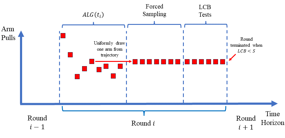
Figure 1: Illustration of a single round of SELECT

Step 1. Identify a Potentially Satisficing Arm: Let $\gamma_{i}=2^{-i(1-\alpha)/\alpha}$, SELECT follows ALG for the first $t_{i}=\lceil\gamma_{i}^{-1/(1-\alpha)}\rceil=\lceil 2^{i/\alpha}\rceil$ steps of round $i$ and records its arm selections. Then, it samples an arm $\hat{X}_{i}$ uniformly random from the trajectory of ALG in this round. By virtue of ALG, we find an arm whose mean reward is at most $\tilde{O}(t^{\alpha-1}_{i})=\tilde{O}(\gamma_{i})$ below $r(X^{*})$ in expectation, and only $\tilde{O}(t^{\alpha}_{i})$ (satisficing) regret is incurred in this step. We note that in the realizable case, as $i$ increases, $\tilde{O}(\gamma_{i})$ will gradually become smaller than $\Delta_{S}^{*}$, meaning that the sampled arm $\hat{X}_{i}$ is more likely to be a satisficing arm and enjoys no satisficing regret;

Step 2. Forced Sampling on the Identified Arm: To validate if $\hat{X}_{i}$ is a satisficing arm or not, we need to collect enough data from pulling $\hat{X}_{i}$ to perform some statistical test on its mean reward. However, when the arm set $\mathcal{X}$ is large, ALG might only have pulled $\hat{X}_{i}$ for limited number of times. To circumvent this, we perform a forced sampling on $\hat{X}_{i}$ by pulling it for $T_{i}=\lceil\gamma^{-2}_{i}\rceil$ times;

Step 3. Lower Confidence Bound Tests: We are now ready to perform the statistical test. In this step, SELECT continues to collect data from $\hat{X}_{i}$. We use $k$ (initialized to 0) to denote the number of additional pieces of noisy reward data generated by pulling $\hat{X}_{i}$ in the current time step and $\hat{r}^{\text{tot}}_{i}$ to denote the running total reward collected from Step 2 and the current step so far. At the same time, it keeps comparing the LCB of $\hat{X}_{i}$’s mean reward, i.e., $\hat{r}^{\text{tot}}_{i}/(T_{i}+k)-\sqrt{4\log(T_{i}+k)/(T_{i}+k)}$, against the threshold value $S$ after acquiring every piece of new data. SELECT terminates this round and enters the next whenever the LCB is less than $S$.

The pseudo-code of SELECT is presented in Algorithm 1.

Remark 2.

We now take a pause to comment on the design of Steps 2 and 3.

1) In Step 3, SELECT compares the LCB of $\hat{X_{i}}$’s mean reward against $S$ to determine if $X_{i}$ is a satisficing arm. This deviates from prior works that use UCB Garivier et al. (2019) or empirical mean Michel et al. (2023). However, it turns out that this is essential in achieving a constant satisficing regret that does not scale with $1/\Delta_{S}$, which can quickly explode in many cases. As we will see, once entering Step 3, SELECT can terminate a round within 1 additional time step in expectation when facing a non-satisficing arm (i.e., (3) in the proof of the forthcoming Proposition 1). In contrast, if it follows prior works to use UCB or empirical mean instead, the number of time steps required (and hence, the satisficing regret) will unavoidably scale with $1/\Delta_{S}$ (see e.g., Theorem 9 of Garivier et al. (2019) or Theorem 1 of Michel et al. (2023));

2) One challenge from using the LCB test in Step 3 is that it is a more conservative design compared to prior works. In fact, if we directly enter Step 3 without Step 2, the LCB of $r(\hat{X_{i}})$ can easily fall below $S$ even if $r(\hat{X}_{i})\geq S$. This is because we may not have pulled $\hat{X}_{i}$ for enough times in Step 1 and the corresponding confidence interval might be large. As a result, the value of $r(\hat{X}_{i})$ LCB, which is the difference between empirical mean and confidence interval, can be extremely small. This indicates, without the forced sampling in Step 2, major satisficing regret can be incurred due to frequent re-start of a new round. With the forced sampled data collected from Step 2, SELECT ensures that the width of the confidence interval is of order $\tilde{O}(T_{i}^{-1/2})=\tilde{O}(\gamma_{i})$ (i.e., same as $\mathbb{E}[r(X^{*})-r(\hat{X}_{i})]$). Consequently, whenever $\gamma_{i}$ shrinks to well below $\Delta_{S}^{*}$, SELECT gradually becomes less likely to terminate a round (see the forthcoming Proposition 2).

Algorithm 1 Satisficing Exploration for General Bandit (SELECT)

Input: time horizon $T$, satisficing level $S$

$\gamma_{i}\leftarrow 2^{-i(1-\alpha)/\alpha}$ for all $i=1,2,3\dots$

for round $i=1,2,\dots$ do

     Set $t_{i}\leftarrow\lceil\gamma_{i}^{-1/(1-\alpha)}\rceil$

     Run $\texttt{ALG}(t_{i})$, let $\{\bar{X}_{s}\}_{s\in[t_{i}]}$ be the trajectory of arm pulls

     Sample $R$ uniformly at random from $\{1,2,\dots,t_{i}\}$ and set $\hat{X}_{i}\leftarrow\bar{X}_{R}$

     Set $T_{i}\leftarrow\lceil\gamma_{i}^{-2}\rceil$, $k\leftarrow 0$

     Let $t$ be the current time step, pull arm $\hat{X}_{i}$ for the next $T_{i}$ time steps, and set $\hat{r}_{i}^{\text{tot}}\leftarrow\sum_{s=t}^{t+T_{i}-1}Y_{s}$

     while $LCB(\hat{X}_{i})\geq S$ do

         Set $k\leftarrow k+1$

         Pull arm $\hat{X}_{i}$ and observe $Y_{t}$, where $t$ is the current time step

         Update $\hat{r}_{i}^{\text{tot}}\leftarrow\hat{r}_{i}^{\text{tot}}+Y_{t}$

         Set

$$LCB(\hat{X}_{i})\leftarrow\dfrac{\hat{r}_{i}^{\text{tot}}}{T_{i}+k}-\sqrt{\dfrac{4\log(T_{i}+k)}{T_{i}+k}}$$

     end while

end for

4 Regret Analysis

In this section, we analyze the regret bounds of SELECT. We begin by providing an upper bound of satisficing regret in the realizable case, i.e., $r(X^{*})\geq S$.

Theorem 1.

Under Assumption 1, if $r(X^{*})\geq S$, then the satisficing regret of SELECT is bounded by

$$\texttt{Regret}_{S}\leq\min\left\{C_{1}^{\frac{1}{1-\alpha}}\left(\dfrac{1}{\Delta_{S}^{*}}\right)^{\frac{\alpha}{1-\alpha}}\cdot\textup{polylog}\left(\dfrac{C_{1}}{\Delta_{S}^{*}}\right),\,C_{1}T^{\alpha}\cdot\textup{polylog}(T)\right\}.$$ (1)

We remark that, from the first term on the RHS of (1), SELECT can achieve a constant (w.r.t. $T$) satisficing regret in the realizable case. Moreover, even when $T$ is relatively small and the constant satisficing regret guarantee is loose compared to the oracle’s regret bound, it is able to adapt to the oracle’s performance.

Proof Sketch..

A complete proof for Theorem 1 is provided in Section A. The proof relies on two critical results. In the first one, we show an upper bound on the satisficing regret of round $i$.

Proposition 1.

If $r(X^{*})\geq S$, then the satisficing regret incurred in round $i$ is bounded by

$$\dfrac{6C_{1}}{(1-\alpha)^{\beta}}\gamma_{i}^{-\alpha/(1-\alpha)}\log(2/\gamma_{i})^{\beta}.$$

The proof of this proposition is provided in Section A.1 of the appendix. We also show that once SELECT runs for enough rounds so that $\gamma_{i}=\tilde{O}(\Delta_{S}^{*})$, it is unlikely to start a new round.

Proposition 2.

If $r(X^{*})\geq S$, then for every $i$ that satisfies

$$\dfrac{32C_{1}}{(1-\alpha)^{\beta}}\gamma_{i}\log(2/\gamma_{i})^{\max\{\beta,1/2\}}\leq\Delta_{S}^{*}\,,$$

the probability that round $i$ ends within the time horizon $T$ (conditioned on the event that round $i$ is started within the time horizon) is bounded by $1/4$.

The proof of this proposition is provided in Section A.2 of the appendix. Since each round of SELECT runs independently, Proposition 2 indicates that the total number of rounds for SELECT can be upper-bounded by a shifted geometric random variable with success rate $3/4$. Combining the results of Proposition 1 and Proposition 2 we are able to establish the statement in Theorem 1. ∎

We also show that, in the non-realizable case, SELECT enjoys the same regret bound as the oracle in Assumption 1 (The proof is provided in Section B of the appendix).

Theorem 2.

Under Assumption 1, if $r(X^{*})<S$, the standard regret of SELECT is bounded by

$$\texttt{Regret}\leq C_{1}T^{\alpha}\cdot\textup{polylog}(T).$$

With the above results, we establish that under a very general assumption, SELECT does achieve constant satisficing regret in the realizable case without compromising the standard regret guarantee in the non-realizable case. Altogether, these empower SELECT the potential to become a general algorithm for decision-making under uncertainty.

5 Examples

In what follows, we instantiate SELECT to several popular bandit optimization settings, including finite-armed bandits, concave bandits, and Lipschitz bandits. Along the way, we showcase how our results enable constant satisficing regret for bandits with large and even infinite arm space, which was not achieved by existing algorithms.

1. Finite-Armed Bandits:

Consider a $K$-armed bandit problem, i.e., $\mathcal{X}=[K]$. In this case, both the UCB algorithm (see, e.g., Bubeck and Cesa-Bianchi (2012)) and Thompson sampling (see, e.g., Agrawal and Goyal (2017)) achieve a regret bound of $O(\sqrt{KT\log(T)})$. Combining them with Theorems 1 and 2, we have the following corollary. At the end of this section, we also provide some discussions on the lower bounds of the satisficing regrets.

Corollary 1.

By using either the UCB algorithm or Thompson sampling as $\texttt{ALG}(\cdot)$, if $r(X^{*})\geq S$, the satisficing regret of SELECT is bounded by

$$\texttt{Regret}_{S}\leq\min\left\{\dfrac{K}{\Delta_{S}^{*}}\cdot\textup{polylog}\left(\dfrac{K}{\Delta_{S}^{*}}\right),\,\sqrt{KT}\cdot\textup{polylog}(T)\right\};$$

If $r(X^{*})<S$, then the standard regret of SELECT is bounded by

$$\texttt{Regret}\leq\sqrt{KT}\cdot\textup{polylog}(T).$$

Remark 3 (Comparison with Garivier et al. (2019), Michel et al. (2023)).

Garivier et al. (2019), Michel et al. (2023) also provide algorithms for satisficing regret for finite-armed bandits. While our satisficing regret bound is incomparable to Garivier et al. (2019), which attains $O(K/\Delta_{S})$ satisficing regret, we provide major improvement over Michel et al. (2023), which achieves $O(K/\Delta_{S}+K/(\Delta_{S}^{*})^{2})$ satisficing regret. Compared to Michel et al. (2023), our regret bound remove the dependence on $\Delta_{S}$ and the additional $1/\Delta_{S}^{*}$ factor. We also point out that if we want to achieve the same satisficing regret as Garivier et al. (2019), we can simply change the LCB test in Step 3 to a UCB test.

2. Concave Bandits:

Consider a concave bandit setting, i.e., $\mathcal{X}\subset\mathcal{R}^{d}$ is a convex set, and $r(X)$ is a concave and $1$-Lipschitz continuous function defined on $\mathcal{X}$. Agarwal et al. (2011) gives an algorithm that enjoys $\text{poly}(d)\sqrt{T}\cdot\text{polylog}(T)$ regret. Together with Theorems 1 and 2, we have the following corollary.

Corollary 2.

By using the algorithm in Agarwal et al. (2011) as $\texttt{ALG}(\cdot)$, if $r(X^{*})\geq S$, then the satisficing regret of SELECT is bounded by

$$\texttt{Regret}_{S}\leq\min\left\{\dfrac{\textup{poly}(d)}{\Delta_{S}^{*}}\cdot\textup{polylog}\left(\dfrac{d}{\Delta_{S}^{*}}\right),\textup{poly}(d)\sqrt{T}\cdot\textup{polylog}(T)\right\};$$

If $r(X^{*})<S$, then the standard regret of SELECT is bounded by

$$\texttt{Regret}\leq\textup{poly}(d)\sqrt{T}\cdot\textup{polylog}(T).$$

3. Lipschitz Bandits:

Consider a Lipschitz bandit setting in $d$ dimensions, i.e., $\mathcal{X}=[0,1]^{d}$, and $r(X)$ is an $L$-Lipschitz function. Slivkins et al. (2019) (see Section 4.2) introduces a UCB algorithm to achieve a $O(L^{1/(d+2)}T^{(d+1)/(d+2)}\log(T)^{1/(d+2)})$ regret upper bound bound. Together with Theorem 1 and Theorem 2, we have the following corollary.

Corollary 3.

By using the UCB algorithm with uniform discretization in Slivkins et al. (2019) as $\texttt{ALG}(\cdot)$, if $r(X^{*})\geq S$, then the satisficing regret of SELECT is bounded by

$$\texttt{Regret}_{S}\leq\min\left\{\dfrac{L}{(\Delta_{S}^{*}/2)^{d+1}}\cdot\textup{polylog}\left(\dfrac{L}{\Delta_{S}^{*}}\right),\,L^{\frac{1}{d+2}}T^{\frac{d+1}{d+2}}\cdot\textup{polylog}(T)\right\};$$

If $r(X^{*})<S$, then the standard regret of SELECT is bounded by

$$\texttt{Regret}\leq L^{\frac{1}{d+2}}T^{\frac{d+1}{d+2}}\cdot\textup{polylog}(T).$$

Remark 4.

Recall that $\Delta_{S}=\min\{S-r(X):r(X)<S\}$, one can easily verify that in the realizable case, $\Delta_{S}=0$ for both concave bandits and the Lipschitz bandits. As such, one cannot directly apply the results in Garivier et al. (2019), Michel et al. (2023) to acquire a constant satisficing regret. With the notion of exceeding gap $\Delta_{S}^{*}$ and SELECT, we establish constant satisficing regret bounds for these two settings.

4. Lower Bounds:

To complement our main results, we also present the satisficing regret lower bounds for finite-armed bandits and concave bandits. The first one is a satisficing regret lower bound for the finite-armed bandits.

Theorem 3 (Finite-Armed Bandits).

For every non-anticipatory learning algorithm $\pi$, every $\Delta>0$ and $T\geq 1/\Delta^{2}$, there exists an instance of two-armed bandit such that $r(X^{*})-S=\Delta$, and the satisficing regret incurred by $\pi$ is at least $\Omega(1/\Delta)$.

Remark 5.

In Michel et al. (2023), the authors adapt the results from Bubeck et al. (2013) (for MAB with known optimal mean reward) to establish a $\Omega(1/\Delta_{S})$ satisficing regret lower bound for finite-armed bandits. This is different than the one in Theorem3, which is $\Omega(1/\Delta)$ with $\Delta$ being the exceeding gap (i.e., $\Delta_{S}^{*}$). This difference originates from the lower bound instances. The lower bound instance in Bubeck et al. (2013) (when adapted to satisficing bandits) sets the threshold value to the optimal mean reward, i.e., $S=r(X^{*})\,,$ which makes both the satisficing regret and standard regret lower bounds to be $\Omega(1/\Delta_{S})$. In our lower bound proof, we allow $S$ to be smaller than $r(X^{*})$, which leads to a lower bound that depends on the difference between these two quantities.

Next, we provide a satisficing regret lower bound for bandits with concave rewards.

Theorem 4 (Bandits with Concave Rewards).

For every non-anticipatory learning algorithm $\pi$, every $\Delta>0$ and every $T\geq 1/\Delta^{2}$, there exists an instance of $1$-dimensional bandit with concave reward such that $r(X^{*})-S=\Delta$, and the satisficing regret incurred by $\pi$ is at least $\Omega(1/\Delta)$.

6 Numerical Experiments

In this section, we conduct numerical experiments to test the performance of SELECT on finite-armed bandits, concave bandits, and Lipschitz bandits. All experiments are run on a PC with 4-core CPU and 16GB of RAM.

6.1 Finite-Armed Bandits

Setup: In this case, we consider an instance of $4$ arms, and the expected rewards of all arms are $\{0.6,0.7,0.8,1\}$. The length of the time horizon is set to be $500$ to $5000$ with a stepsize of $500$. We conduct experiments for both the realizable case and the non-realizable case. For the realizable case, we set the satisficing level $S=0.93$; for the non-realizable case, we set the satisficing level $S=1.5$. In both cases, we compare SELECT against Thompson sampling in Agrawal and Goyal (2017) as well as SAT-UCB and SAT-UCB+ in Hajiabolhassan and Ortner (2023). The experiment is repeated for 1000 times and we report the average results.

Results: The results of the realizable case is presented in Figure 2(a), and the results of the non-realizable case is presented in Figure 2(b). From Figure 2(a) one can see that SELECT, SAT-UCB and SAT-UCB+ exhibit constant satisficing regret, and incur less satisficing regret compared to Thompson sampling. Furthermore, SELECT incurs less regret compared to SAT-UCB and achieves comparable performance with SAT-UCB+ in the realizable case. From Figure 2(b) one can see that SELECT incurs roughly the same standard regret as Thompson sampling. Furthermore, SELECT also incurs less standard regret in the non-realizable case compared to either SAT-UCB or SAT-UCB+.

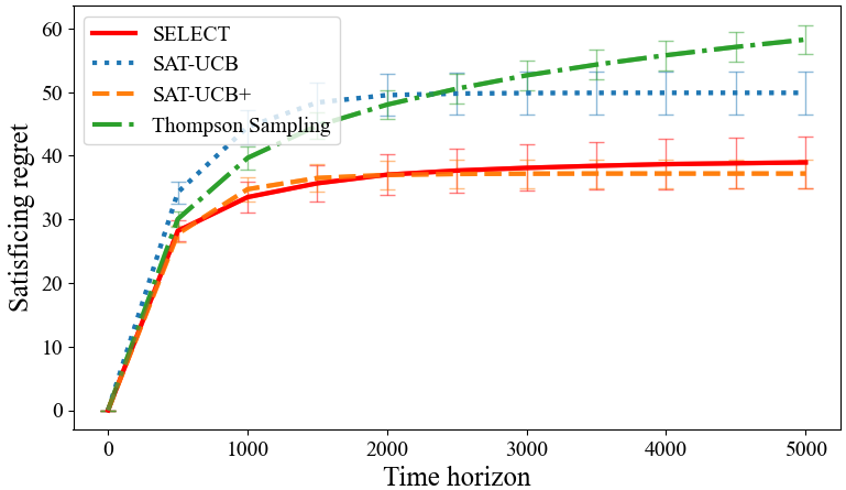
(a) Satisficing Regret in the Realizable Case

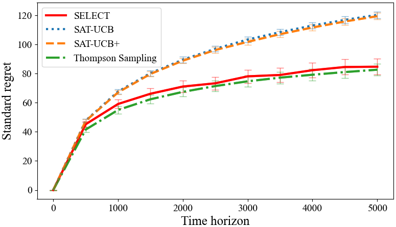
(b) Standard Regret in the Non-Realizable Case

Figure 2: Comparison of SELECT , Thompson sampling, SAT-UCB and SAT-UCB+

6.2 Concave Bandits

Setup: In this case, we consider an instance with arm set $[0,1]$ and concave reward function $r(x)=1-16(x-0.25)^{2}$. The length of the time horizon is set to be $500$ to $5000$ with a stepsize of $500$. We consider both the realizable case and the non-realizable case. For the realizable case, we set the satisficing level $S=0.3$; for the non-realizable case, we set the satisficing level $S=1.5$. For both cases, we compare our algorithm SELECT with the convex bandit algorithm introduced in Agarwal et al. (2011). We also use SAT-UCB and SAT-UCB+ as heuristics by viewing the problem as Lipschitz bandits. That is, we first discretize the arm space uniformly with stepsize $L^{1/3}T^{-1/3}$, where $L$ is the Lipschitz constant of the reward function, and then run SAT-UCB and SAT-UCB+ over the discretized arm space. The experiment is repeated for 1000 times and we report the average results.

Results: The results of realizable case is provided in Figure 3(a), and the results of non-realizable case is provided in Figure 3(b). From Figure 3(a), we can see that SELECT converges to satisficing arms faster and incurs smaller satisficing regret than the algorithm in Agarwal et al. (2011), SAT-UCB and SAT-UCB+. The reason why SAT-UCB and SAT-UCB+ has not converged is that they usually repeatedly pull non-satisficing arms which are close to satisficing level but provide empirically highest UCB. As shown in Figure 3(b), SELECT can also reach good enough distribution compared to the algorithm in Agarwal et al. (2011) , SAT-UCB, and SAT-UCB+ in the non-realizable case.

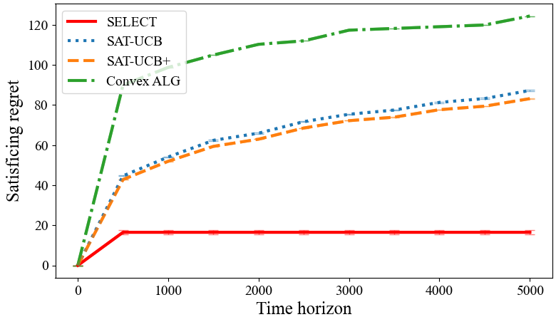
(a) Satisficing Regret in the Realizable Case

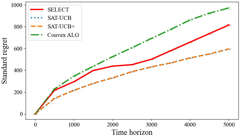
(b) Standard Regret in the Non-Realizable Case

Figure 3: Comparison of  SELECT , Stochastic Convex, SAT-UCB and SAT-UCB+ for concave bandit

6.3 Lipschitz Bandits

Setup: In this case, we consider a two-dimensional Lipschitz bandit in domain $(x,y)\in[0,1]^{2}$ with Lipschitz rewards $f(x,y)=\min\{1,3e^{-100((x-0.5)^{2}+(y-0.7)^{2})}\}$. The length of the time horizon is set to be $500$ to $5000$ with a stepsize of $500$. We consider both the realizable case and the non-realizable case. For the realizable case, we set the satisficing level S = 0.5; for the non-realizable case, we set the satisficing level S = 1.5. For both cases, we compare our algorithm SELECT with the uniformly discretized UCB introduced in Slivkins et al. (2019). We again use SAT-UCB and SAT-UCB+ as heuristics by uniformly discretizing the arm space with stepsize $L^{1/3}T^{-1/3}$, where $L$ is the Lipschitz constant of the reward function, and run the algorithms over the discretized arms. The experiment is repeated for 1000 times and we report the average results.

Results: The results of realizable case is provided in Figure 4(a), and the results of non-realizable case is provided in Figure 4(b). From Figure 4(a), we can see that SELECT converges to satisficing arms faster and incurs smaller satisficing regret than uniform UCB, SAT-UCB and SAT-UCB+. From 4(b), we can see that SELECT still works the best while Uniform UCB, SAT-UCB and SAT-UCB+ have similar performance.

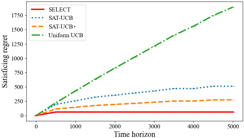
(a) Satisficing Regret in the Realizable Case

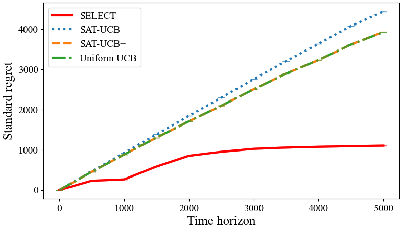
(b) Standard Regret in the Non-Realizable Case

Figure 4: Comparison of  SELECT , Uniform UCB, SAT-UCB and SAT-UCB+ for Lipschitz bandit

7 Conclusion

In this paper, we propose SELECT, a general algorithmic template, for satisficing exploration in bandit optimization. For a given bandit optimization problem and a sub-linear regret learning oracle, we show that SELECT attains constant satisficing regret in the realizable case and the same regret as the learning oracle in the non-realizable case. We instantiate SELECT to finite-armed bandits, concave bandits, and Lipschitz bandits, and also make a discussion on the corresponding lower bounds. Finally, numerical experiments show that SELECT attains constant regret in several popular bandit problems and demonstrates excellent performances when compared to other benchmarks in both the realizable and the non-realizable cases.

Appendix A Proof of Theorem 1

Denote $\beta^{\prime}=\max\{\beta,1/2\}$ and $K_{\alpha,\beta}=\dfrac{32}{(1-\alpha)^{\beta}}$, and $i_{0}$ as

$$i_{0}=\max\{i:C_{1}K_{\alpha,\beta}\gamma_{i}\log(2/\gamma_{i})^{\max\{\beta,1/2\}}>\Delta_{S}^{*}\}.$$

We first prove an upper bound on $i_{0}$. Denote $\delta_{0}\in(0,1)$ the smallest solution to the following equation

$$\delta_{0}\log(2/\delta_{0})^{\beta^{\prime}}=\dfrac{\Delta_{S}^{*}}{C_{1}K_{\alpha,\beta}}.$$

Then we have

$$\dfrac{1}{\delta_{0}}=\dfrac{C_{1}K_{\alpha,\beta}\log(1/\delta_{0})^{\beta^{\prime}}}{\Delta_{S}^{*}}=\dfrac{(4\beta^{\prime})^{\beta^{\prime}}C_{1}C_{\alpha,\beta}\log(2/\delta_{0}^{1/4\beta^{\prime}})^{\beta^{\prime}}}{\Delta_{S}^{*}}\leq\dfrac{(8\beta^{\prime})^{\beta^{\prime}}C_{1}K_{\alpha,\beta}}{\Delta_{S}^{*}(\delta_{0})^{1/4}},$$

or equivalently

$$\dfrac{1}{\delta_{0}}\leq\left(\dfrac{(8\beta^{\prime})^{\beta^{\prime}}C_{1}K_{\alpha,\beta}}{\Delta_{S}^{*}}\right)^{4/3},$$

therefore

$$\dfrac{1}{\delta_{0}}\leq\dfrac{(4/3)^{\beta^{\prime}}C_{1}K_{\alpha,\beta}\log({2(8\beta^{\prime})^{\beta^{\prime}}C_{1}K_{\alpha,\beta}}/{\Delta_{S}^{*}})^{\beta^{\prime}}}{\Delta_{S}^{*}}$$

We write $D_{\alpha,\beta}=2(8\beta^{\prime})^{\beta^{\prime}}K_{\alpha,\beta}$, $L_{\alpha,\beta}=(4/3)^{\beta^{\prime}}K_{\alpha,\beta}$, then we have

$$\delta_{0}\geq\dfrac{\Delta_{S}^{*}}{L_{\alpha,\beta}C_{1}\log(D_{\alpha,\beta}C_{1}/\Delta_{S}^{*})^{\beta^{\prime}}}.$$

By definition of $i_{0}$ we also have

$$\gamma_{i_{0}}\geq\dfrac{\Delta_{S}^{*}}{L_{\alpha,\beta}C_{1}\log(D_{\alpha,\beta}C_{1}/\Delta_{S}^{*})^{\beta^{\prime}}},$$

thus

$$i_{0}\leq\dfrac{\alpha}{1-\alpha}\log_{2}\left(\dfrac{L_{\alpha,\beta}C_{1}\log(D_{\alpha,\beta}C_{1}/\Delta_{S}^{*})^{\beta^{\prime}}}{\Delta_{S}^{*}}\right).$$

Using the result of Proposition 1 we have that the satisficing regret by round $i_{0}$ is bounded by

$$\sum_{i=1}^{i_{0}}\dfrac{6C_{1}}{(1-\alpha)^{\beta}}\gamma_{i}^{-\alpha/(1-\alpha)}\log(2/\delta_{0})^{\beta}$$

$$= \sum_{i=1}^{i_{0}}\dfrac{6C_{1}}{(1-\alpha)^{\beta}}2^{i}\log(2/\delta_{0})^{\beta}$$

$$= \dfrac{12C_{1}}{(1-\alpha)^{\beta}}2^{i_{0}}\log(2/\delta_{0})^{\beta}$$

$$\leq \dfrac{16C_{1}}{(1-\alpha)^{\beta}}\left(\dfrac{L_{\alpha,\beta}C_{1}\log(D_{\alpha,\beta}C_{1}/\Delta_{S}^{*})^{\beta^{\prime}}}{\Delta_{S}^{*}}\right)^{\alpha/(1-\alpha)}\log\left(\dfrac{D_{\alpha,\beta}C_{1}}{\Delta_{S}^{*}}\right)$$

$$= \dfrac{16L_{\alpha,\beta}^{\alpha/(1-\alpha)}C_{1}^{1/(1-\alpha)}}{(1-\alpha)^{\beta}}\left(\dfrac{1}{\Delta_{S}^{*}}\right)^{\alpha/(1-\alpha)}\log\left(\dfrac{D_{\alpha,\beta}C_{1}}{\Delta_{S}^{*}}\right)^{\alpha\beta^{\prime}/(1-\alpha)+1}.$$

By the results of Proposition 2, for every $k\geq 1$, the probability that round $i_{0}+k$ starts within the time horizon is at most $4^{-k+1}$. Therefore the regret incurred after round $i_{0}$ is bounded by

$$\sum_{k=1}^{\infty}\dfrac{6C_{1}}{(1-\alpha)^{\beta}}2^{i_{0}+k}\log(2/\gamma_{i})^{\beta}\cdot 4^{-k+1}$$

$$\leq \dfrac{12C_{1}}{(1-\alpha)^{\beta}}2^{i_{0}}\log(2/\delta_{0})^{\beta}\cdot\sum_{k=1}^{\infty}k^{\beta}\cdot 2^{-k}$$

$$\leq \dfrac{8L_{\alpha,\beta}^{\alpha/(1-\alpha)}C_{1}^{1/(1-\alpha)}M_{\beta}}{(1-\alpha)^{\beta}}\left(\dfrac{1}{\Delta_{S}^{*}}\right)^{\alpha/(1-\alpha)}\log\left(\dfrac{D_{\alpha,\beta}C_{1}}{\Delta_{S}^{*}}\right)^{\alpha\beta^{\prime}/(1-\alpha)+1},$$

where $M_{\beta}=\sum_{k=1}^{\infty}k^{\beta}\cdot 2^{-k}$, and the total satisficing regret is bounded by

$$\texttt{Regret}_{S}\leq\dfrac{8L_{\alpha,\beta}^{\alpha/(1-\alpha)}C_{1}^{1/(1-\alpha)}(M_{\beta}+2)}{(1-\alpha)^{\beta}}\left(\dfrac{1}{\Delta_{S}^{*}}\right)^{\alpha/(1-\alpha)}\log\left(\dfrac{D_{\alpha,\beta}C_{1}}{\Delta_{S}^{*}}\right)^{\alpha\beta^{\prime}/(1-\alpha)+1}.$$

Furthermore, since the length of the time horizon is $T$ time steps, we have $t_{i}\leq T$, thus the maximum number of rounds is bounded by $i_{\max}=\lceil\alpha\log_{2}(T)\rceil$. By the results of Proposition 1 we have that the satisficing regret is bounded by

$$\texttt{Regret}_{S}\leq \sum_{i=1}^{i_{\max}}\dfrac{6C_{1}}{(1-\alpha)^{\beta}}\gamma_{i}^{-\alpha/(1-\alpha)}\log(2T)^{\beta}$$

$$\leq \sum_{i=1}^{i_{\max}}\dfrac{6C_{1}}{(1-\alpha)^{\beta}}2^{i+1}\log(2T)^{\beta}$$

$$\leq \dfrac{24C_{1}}{(1-\alpha)^{\beta}}T^{\alpha}\log(2T)^{\beta}.$$

Combining the two parts of results we have completed the proof of Theorem 1.

A.1 Proof of Proposition 1

Recall that $t_{i}=\lceil\gamma_{i}^{-1/(1-\alpha)}\rceil\,,$ the satisficing regret incurred when running $\texttt{ALG}(t_{i})$ is bounded by

$$\mathbb{E}\left[\sum_{s=1}^{t_{i}}\max\{S-r(X_{s}),0\}\right]\leq\mathbb{E}\left[t_{i}r(X^{*})-\sum_{s=1}^{t_{i}}r(X_{s})\right]\leq C_{1}t_{i}^{\alpha}\log(t_{i})^{\beta}$$

$$\leq \dfrac{2C_{1}}{(1-\alpha)^{\beta}}\gamma_{i}^{-\alpha/(1-\alpha)}\log(2/\gamma_{i})^{\beta}.$$

Since $\hat{X}_{i}$ is selected randomly according to the trajectory of $\texttt{ALG}(t_{i})$ in round $i$, we further have

$$\mathbb{E}[\max\{S-r(\hat{X}_{i}),0\}]\leq\mathbb{E}[r(X^{*})-r(\hat{X}_{i})]= \frac{\mathbb{E}\left[t_{i}r(X^{*})-\sum_{s=1}^{t_{i}}r(X_{s})\right]}{t_{i}}$$

$$\leq \dfrac{2C_{1}}{(1-\alpha)^{\beta}}\gamma_{i}\log(2/\gamma_{i})^{\beta}.$$

Therefore the satisficing regret incurred when pulling $\hat{X}_{i}$ for $T_{i}=\lceil\gamma_{i}^{-2}\rceil$ times is bounded by

$$\left\lceil\dfrac{1}{\gamma_{i}^{2}}\right\rceil\cdot\dfrac{2C_{1}}{(1-\alpha)^{\beta}}\gamma_{i}\log(2/\gamma_{i})^{\beta}=\dfrac{3C_{1}}{(1-\alpha)^{\beta}}\gamma_{i}^{-1}\log(2/\gamma_{i})^{\beta}\leq\dfrac{3C_{1}}{(1-\alpha)^{\beta}}\gamma_{i}^{-\alpha/(1-\alpha)}\log(2/\gamma_{i})^{\beta}.$$

If $r(\hat{X}_{i})<S$, then for every $k$, round $i$ is not terminated after pulling arm $\hat{X}_{i}$ for $k$ times (in addition to the first $T_{i}$ times) occurs with probability at most

$$\text{Pr}\left(\dfrac{\hat{r}^{\text{tot}}_{i}}{T_{i}+k}-\sqrt{\dfrac{4\log(T_{i}+k)}{T_{i}+k}}>S\right)$$

$$\leq \text{Pr}\left(\dfrac{\hat{r}^{\text{tot}}_{i}}{T_{i}+k}-\sqrt{\dfrac{4\log(T_{i}+k)}{T_{i}+k}}>r(\hat{X}_{i})\right)$$

$$\leq \dfrac{1}{(T_{i}+k)^{2}}\leq\dfrac{1}{(k+8)^{2}}.$$ (2)

Therefore expected number of arm pulls of $\hat{X}_{i}$ after first pulling it $T_{i}$ times is bounded by

$$\mathbb{E}\left[\text{Number of times }\hat{X}_{i}\text{ is pulled in round }i\text{ after the first }T_{i}\text{ times}\right]$$

$$= \sum_{s=1}^{\infty}\text{Pr}(k\geq s)=\sum_{s=1}^{\infty}\dfrac{1}{(s+8)^{2}}\leq 1.$$ (3)

Summing up the three parts of satisficing regret we have that the satisficing regret of round $i$ is bounded by

$$\dfrac{6C_{1}}{(1-\alpha)^{\beta}}\gamma_{i}^{-\alpha/(1-\alpha)}\log(2/\gamma_{i})^{\beta}.$$

A.2 Proof of Proposition 2

We denote $X^{*}=\arg\max_{X\in\mathcal{X}}r(X)$.

By Assumption 1 and recall from the proof of Proposition 1, we have

$$\mathbb{E}[r(X^{*})-r(\hat{X}_{i})]= \dfrac{1}{t_{i}}\mathbb{E}\left[t_{i}r(X^{*})-\sum_{s=1}^{t_{i}}r(X_{s})\right]\leq\dfrac{1}{t_{i}}C_{1}t_{i}^{\alpha}\log(t_{i})^{\beta}=C_{1}t_{i}^{\alpha-1}\log(t_{i})^{\beta}$$

$$\leq \dfrac{2C_{1}}{(1-\alpha)^{\beta}}\gamma_{i}\log(2/\gamma_{i})^{\beta},$$

where the last inequality holds because $t_{i}=\lceil 1/\gamma^{1/(1-\alpha)}\rceil\leq 2/\gamma^{1/(1-\alpha)}$.

According to the assumption of this proposition, we have $i$ satisfies the condition

$$\dfrac{32C_{1}}{(1-\alpha)^{\beta}}\gamma_{i}\log(2/\gamma_{i})^{\max\{\beta,1/2\}}\leq\Delta_{S}^{*},$$

by the Markov’s inequality we have

$$\text{Pr}(r(X^{*})-r(\hat{X}_{i})\geq\Delta_{S}^{*}/2)\leq\text{Pr}\left(r(X^{*})-r(\hat{X}_{i})\geq\dfrac{16C_{1}}{(1-\alpha)^{\beta}}\log(2/\gamma_{i})^{\beta}\right)\leq\dfrac{1}{8}.$$ (4)

Now, if $r(\hat{X}_{i})\geq r(X^{*})-\Delta_{S}^{*}/2$, which happens with probability at least 7/8 according to the above inequality, then $r(\hat{X}_{i})\geq S+\Delta_{S}^{*}/2$ holds. On the other hand, if $i$ satisfies the condition stated in the proposition, then $\gamma_{i}\log(1/\gamma_{i})^{1/2}\leq\Delta_{S}^{*}/16$.

Note that $f(x)=\log(x)/x$ is monotonically decreasing when $x\geq 3$ and $2\cdot\log(2)/2\geq\log(3)/3$, for all $k\geq 0$,

$$\sqrt{\dfrac{{4\log(T_{i}+k)}}{T_{i}+k}}\leq 4\sqrt{\dfrac{\log(T_{i})}{T_{i}}}\leq\dfrac{\Delta_{S}^{*}}{4}.$$

Suppose round $i$ is terminated for some $k$, then

$$\dfrac{\hat{r}_{i}^{\text{tot}}}{T_{i}+k}-\sqrt{\dfrac{4\log(T_{i}+k)}{T_{i}+k}}<S=r(X^{*})-\Delta_{S}^{*}\leq r(\hat{X}_{i})-\dfrac{\Delta_{S}^{*}}{2}\leq r(\hat{X}_{i})-2\sqrt{\dfrac{4\log(T_{i}+k)}{T_{i}+k}},$$

or equivalently

$$\dfrac{\hat{r}_{i}^{\text{tot}}}{T_{i}+k}\leq r(\hat{X}_{i})-\sqrt{\dfrac{4\log(T_{i}+k)}{T_{i}+k}}.$$

By the Hoeffding’s inequality we have

$$\text{Pr}\left(\dfrac{\hat{r}_{i}^{\text{tot}}}{T_{i}+k}\leq r(\hat{X}_{i})-\sqrt{\dfrac{4\log(T_{i}+k)}{T_{i}+k}}\right)\leq\dfrac{1}{(T_{i}+k)^{2}}\leq\dfrac{1}{(k+4)^{2}}.$$

Therefore conditioned on $r(\hat{X}_{i})\geq r(X^{*})-\Delta_{S}^{*}/2$ the probability that round $i$ is terminated by the end of the horizon is bounded by

$$\sum_{k=1}^{\infty}\dfrac{1}{(k+8)^{2}}\leq\dfrac{1}{8}.$$ (5)

Combining (4) and (5) we conclude that the probability that round $i$ terminates by the end of the time horizon is bounded by $1/4$.

Appendix B Proof of Theorem 2

We first prove that the regret incurred in round $i$ is at most

$$\dfrac{6C_{1}}{(1-\alpha)^{\beta}}\gamma_{i}^{-\alpha/(1-\alpha)}\log(2/\gamma_{i})^{\beta}.$$

The regret incurred when running $\texttt{ALG}(t_{i})$ is bounded by

$$\mathbb{E}\left[\sum_{s=1}^{t_{i}}\max\{S-r(X_{s}),0\}\right]\leq\mathbb{E}\left[t_{i}r(X^{*})-\sum_{s=1}^{t_{i}}r(X_{s})\right]\leq C_{1}t_{i}^{\alpha}\log(t_{i})^{\beta}\leq\dfrac{2C_{1}}{(1-\alpha)^{\beta}}\gamma_{i}^{-\alpha/(1-\alpha)}\log(2/\gamma_{i})^{\beta}.$$

We further have

$$\mathbb{E}[r(X^{*})-r(\hat{X}_{i})]\leq\dfrac{2C_{1}}{(1-\alpha)^{\beta}}\gamma_{i}\log(2/\gamma_{i})^{\beta}.$$

Therefore the satisficing regret incurred when pulling $\hat{X}_{i}$ is bounded by

$$\left\lceil\dfrac{1}{\gamma_{i}^{2}}\right\rceil\cdot\dfrac{2C_{1}}{(1-\alpha)^{\beta}}\gamma_{i}\log(2/\gamma_{i})^{\beta}=\dfrac{3C_{1}}{(1-\alpha)^{\beta}}\gamma_{i}^{-1}\log(2/\gamma_{i})^{\beta}\leq\dfrac{3C_{1}}{(1-\alpha)^{\beta}}\gamma_{i}^{-\alpha/(1-\alpha)}\log(2/\gamma_{i})^{\beta}.$$

Since $r(\hat{X}_{i})\leq r(X^{*})<S$, for every $k$, round $i$ is not terminated with probability at most

$$\text{Pr}\left(\dfrac{\hat{r}^{\text{tot}}_{i}}{T_{i}+k}-\sqrt{\dfrac{4\log(T_{i}+k)}{T_{i}+k}}>S\right)$$

$$\leq \text{Pr}\left(\dfrac{\hat{r}^{\text{tot}}_{i}}{T_{i}+k}--\sqrt{\dfrac{4\log(T_{i}+k)}{T_{i}+k}}>r(\hat{X}_{i})\right)$$

$$\leq \dfrac{1}{(T_{i}+k)^{2}}\leq\dfrac{1}{(k+8)^{2}}.$$

Therefore expected number of arm pulls of $\hat{X}_{i}$ after pulling $T_{i}$ times is bounded by

$$\sum_{k=1}^{\infty}\dfrac{1}{(k+8)^{2}}\leq 1.$$

Summing up the three parts of regret we have that the satisficing regret of round $i$ is bounded by

$$\dfrac{6C_{1}}{(1-\alpha)^{\beta}}\gamma_{i}^{-\alpha/(1-\alpha)}\log(2/\gamma_{i})^{\beta}.$$

Since the length of the time horizon is $T$ time steps, we have $t_{i}\leq T$, thus the maximum number of rounds is bounded by $i_{\max}=\lceil\alpha\log_{2}(T)\rceil$. Therefore we have that the regret is bounded by

$$\texttt{Regret}_{S}\leq \sum_{i=1}^{i_{\max}}\dfrac{6C_{1}}{(1-\alpha)^{\beta}}\gamma_{i}^{-\alpha/(1-\alpha)}\log(2T)^{\beta}$$

$$\leq \sum_{i=1}^{i_{\max}}\dfrac{6C_{1}}{(1-\alpha)^{\beta}}2^{i+1}\log(2T)^{\beta}$$

$$\leq \dfrac{24C_{1}}{(1-\alpha)^{\beta}}T^{\alpha}\log(2T)^{\beta}.$$

Therefore the regret is bounded by $C_{1}T^{\alpha}\cdot\text{polylog}(T)$.

Appendix C Proofs for Lower Bounds

C.1 Proof of Theorem 3

Denote $T_{0}=\lceil 1/\Delta^{2}\rceil$. We consider the following instances of two-armed bandit:

$$\textbf{Instance 1:}\ r^{(1)}(1)=\Delta,\ r^{(1)}(2)=-\Delta;\ \textbf{Instance 2:}\ r^{(2)}(1)=-\Delta,\ r^{(2)}(2)=\Delta.$$

We further set the satisficing level $S=0$, and assume that noise $\epsilon_{t}$ follows i.i.d. standard normal distribution. Then for any $t\in[T_{0}]$,

$$\texttt{KL}\left(\text{Pr}_{t}^{(1)}||\text{Pr}_{t}^{(2)}\right)=(t-1)\,\texttt{KL}(N(\Delta,1)||N(-\Delta,1))=\dfrac{t\Delta^{2}}{2}\leq\dfrac{\Delta^{2}}{2}\cdot\dfrac{1}{\Delta^{2}}=\dfrac{1}{2}.$$

We denote $\texttt{Regret}_{S}^{(i)}$ as the satisficing regret under instance $i$. Then by the Bretagnolle-Huber inequality (see, e.g., Theorem 14.2 of Lattimore and Szepesvári (2020)), we have

$$\texttt{Regret}_{S}^{(1)}+\texttt{Regret}_{S}^{(2)}\geq \Delta\sum_{t=1}^{T_{0}}\text{Pr}_{t}^{(1)}(X_{t}=2)+\text{Pr}_{t}^{(2)}(X_{t}=1)$$

$$\geq T_{0}\Delta\cdot\exp\left(-\texttt{KL}\left(\text{Pr}_{t}^{(1)}||\text{Pr}_{t}^{(2)}\right)\right)\geq\Delta\cdot\dfrac{1}{\Delta^{2}}\cdot\exp\left(-\dfrac{1}{2}\right)$$

$$= \Omega\left(\dfrac{1}{\Delta}\right).$$

Therefore any non-anticipatory learning algorithm will incur at least $\Omega(1/\Delta)$ satisficing regret under one of the two instances.

C.2 Proof of Theorem 4

Assume without loss of generality that $\Delta\leq 1$. Denote $T_{0}=\lceil 1/16\Delta^{2}\rceil$. We consider the following instances of two-armed bandit: $\mathcal{X}=[-3,3]$, and reward function is defined as follows:

$$\textbf{Instance 1:}\ r^{(1)}(x)=\max\{20x+40\sqrt{2\Delta}+1-2\Delta,\,1-(x+\sqrt{2\Delta})^{2},\,-20x+40\sqrt{2\Delta}+1-2\Delta\},$$

$$\textbf{Instance 2:}\ r^{(2)}(x)=\max\{20x+40\sqrt{2\Delta}+1-2\Delta,\,1-(x-\sqrt{2\Delta})^{2},\,-20x+40\sqrt{2\Delta}+1-2\Delta\}.$$

We further set satisficing level $S=1-\Delta$, and assume that the noise $\epsilon_{t}$ follows i.i.d. standard normal distribution.

It is easy to verify that $|r^{(1)}(x)-r^{(2)}(x)|$ obtains its maximum at $-2\sqrt{2\Delta}$ and $2\sqrt{2\Delta}$, and

$$|r^{(1)}(\sqrt{2\Delta})-r^{(2)}(\sqrt{2\Delta})|=2\sqrt{2\Delta}\cdot 2\sqrt{2\Delta}=8\Delta.$$

Therefore for any $t\in[T_{0}]$,

$$\texttt{KL}\left(\text{Pr}_{t}^{(1)}||\text{Pr}^{(2)}_{t}\right)\leq(t-1)\cdot\dfrac{(8\Delta)^{2}}{2}\leq\dfrac{1}{16\Delta^{2}}\cdot 32\Delta^{2}=2.$$

We denote $\texttt{Regret}_{S}^{(i)}$ as the satisficing regret under instance $i$, then by the Bretagnolle-Huber inequality (see, e.g., Theorem 14.2 of Lattimore and Szepesvári (2020)), we have

$$\texttt{Regret}_{S}^{(1)}+\texttt{Regret}_{S}^{(2)} \geq\Delta\sum_{t=1}^{T_{0}}\text{Pr}_{t}^{(1)}(X_{t}\geq 0)+\text{Pr}_{t}^{(2)}(X_{t}\leq 0)$$

$$\geq T_{0}\Delta\cdot\exp\left(-\texttt{KL}\left(\text{Pr}_{t}^{(1)}||\text{Pr}_{t}^{(2)}\right)\right)$$

$$\geq T_{0}\Delta\cdot\exp(-2)=\dfrac{\exp(-2)}{16\Delta^{2}}\cdot\Delta=\Omega(1/\Delta).$$

Therefore any non-anticipatory learning algorithm will incur at least $\Omega(1/\Delta)$ in one of the two instances.

References

- Abernethy et al. (2016) Abernethy, Jacob, Kareem Amin, Ruihao Zhu. 2016. Threshold bandits, with and without censored feedback. Advances in Neural Information Processing Systems 29.
- Agarwal et al. (2011) Agarwal, Alekh, Dean P Foster, Daniel J Hsu, Sham M Kakade, Alexander Rakhlin. 2011. Stochastic convex optimization with bandit feedback. Advances in Neural Information Processing Systems 24.
- Agrawal and Goyal (2017) Agrawal, Shipra, Navin Goyal. 2017. Near-optimal regret bounds for thompson sampling. Journal of the ACM (JACM) 64(5) 1–24.
- Aransiola (2023) Aransiola, Olayemi Jemimah. 2023. What is satisficing and how it affects survey results. Formplus .
- Bubeck and Cesa-Bianchi (2012) Bubeck, Sébastien, Nicolo Cesa-Bianchi. 2012. Regret analysis of stochastic and nonstochastic multi-armed bandit problems. Foundations and Trends® in Machine Learning 5(1) 1–122.
- Bubeck et al. (2013) Bubeck, Sébastien, Vianney Perchet, Philippe Rigollet. 2013. Bounded regret in stochastic multi-armed bandits. Conference on Learning Theory. PMLR, 122–134.
- Garivier et al. (2019) Garivier, Aurélien, Pierre Ménard, Gilles Stoltz. 2019. Explore first, exploit next: The true shape of regret in bandit problems. Mathematics of Operations Research 44(2) 377–399.
- Hajiabolhassan and Ortner (2023) Hajiabolhassan, Hossein, Ronald Ortner. 2023. Online regret bounds for satisficing in mdps. Sixteenth European Workshop on Reinforcement Learning.
- Jenkins (2022) Jenkins, Abby. 2022. Safety stock: What it is & how to calculate. Oracle NetSuite .
- Lattimore and Szepesvári (2020) Lattimore, Tor, Csaba Szepesvári. 2020. Bandit algorithms. Cambridge University Press.
- Lufkin (2021) Lufkin, Bryan. 2021. Do ’maximisers’ or ’satisficers’ make better decisions? BBC .
- Mabey (2022) Mabey, Chris. 2022. Optimizing vs satisficing: Tips for product design and designing your life. The BYU Design Review .
- Michel et al. (2023) Michel, Thomas, Hossein Hajiabolhassan, Ronald Ortner. 2023. Regret bounds for satisficing in multi-armed bandit problems. Transactions on Machine Learning Research .
- Reverdy and Leonard (2014) Reverdy, Paul, Naomi E Leonard. 2014. Satisficing in gaussian bandit problems. 53rd IEEE Conference on Decision and Control. IEEE, 5718–5723.
- Reverdy et al. (2017) Reverdy, Paul, Vaibhav Srivastava, Naomi Ehrich Leonard. 2017. Satisficing in multi-armed bandit problems. IEEE Transactions on Automatic Control 62(8) 3788–3803.
- Russo and Van Roy (2022) Russo, Daniel, Benjamin Van Roy. 2022. Satisficing in time-sensitive bandit learning. Mathematics of Operations Research 47(4) 2815–2839.
- Simon (1956) Simon, Herbert A. 1956. Rational choice and the structure of the environment. Psychological Review .
- Slivkins et al. (2019) Slivkins, Aleksandrs, et al. 2019. Introduction to multi-armed bandits. Foundations and Trends® in Machine Learning 12(1-2) 1–286.
- Tamatsukuri and Takahashi (2019) Tamatsukuri, Akihiro, Tatsuji Takahashi. 2019. Guaranteed satisficing and finite regret: Analysis of a cognitive satisficing value function. Biosystems 180 46–53.
- Vandeput (2021) Vandeput, Nicolas. 2021. Inventory optimization: 5 ways to set service level and safety stock targets. Medium .
- Whitenton (2014) Whitenton, Kathryn. 2014. Satisficing: Quickly meet users’ main needs. Nielsen Norman Group .
- Willemain (2017) Willemain, Thomas. 2017. How to choose a target service level. Smart Software .