Landscape estimates of the integrated density of states for Jacobi operators on graphs
Abstract.
We show the integrated density of states for a variety of Jacobi operators on graphs, such as the Anderson model and random hopping models on graphs with Gaussian heat kernel bounds, can be estimated from above and below in terms of the localization landscape counting function. Specific examples of these graphs include stacked and decorated lattices, graphs corresponding to band matrices, and aperiodic tiling graphs. The upper bound part of the landscape law also applies to the fractal Sierpinski gasket graph. As a consequence of the landscape law, we obtain landscape-based proofs of the Lifshitz tails in several models including random band matrix models, certain bond percolation Hamiltonians on , and Jacobi operators on certain stacks of graphs. We also present intriguing numerical simulations exploring the behavior of the landscape counting function across various models.
1. Introduction
The structure and dynamics of quantum systems for electrons are generally described using a Hamiltonian operator. The simplified non-interacting Hamiltonian of a crystalline solid can often be modeled by a graph operator , which is a weighted graph Laplacian perturbed by an on-site potential. The integrated density of states (IDS) of is one of the main quantities encoding the energy levels of the system. It describes the number of energy levels per unit volume below a certain energy level. In the present work, we establish bounds on the IDS of via the counting function of the so-called localization landscape [14]. Such a Landscape Law approach was first established in [9] for the standard Schrödinger operator on , and later extended to in [1, 10].
The goal of the present paper is to establish the landscape law for more general graph operators with both on-site potential and bond interactions. This extension is in two directions: First, by moving to graphs, we lose the regular structure of and used in [9, 1] to perform partition and translation arguments. Second, by allowing for disordered bond interactions, we extend the class of operators to include random hopping and Jacobi operators, which may have degenerate off-diagonal hopping amplitudes. The resulting landscape law will apply to a range of models, including Jacobi operators on graphs roughly isometric to (or more generally, graphs with Gaussian heat kernel bounds), which includes stacked and decorated lattices, graphs corresponding to banded matrices, and aperiodic tiling graphs. We also obtain a landscape law upper bound for the Sierpinski gasket graph, which is not roughly isometric to any and has non-Gaussian (specifically, sub-Gaussian) heat kernel bounds.
After establishing the landscape law, the general method described in [9, 1] will allow us to recover Lifshitz tail estimates for several of the random hopping models on , including random band matrices, bond percolation Hamiltonians with certain boundary conditions, and discrete acoustic operators . This provides alternate proofs, using the landscape function, for Lifshitz tails in these models (cf. [24, 31, 30, 25, 37]). The landscape law method here also suggests an avenue to obtain Lifshitz tails for non-regular graphs, if one proves certain geometric properties of the graphs.
We now introduce some definitions in order to state our main results. We consider an (unweighted) graph , where the vertex set is countably infinite. We write to mean , and in this case say that is a neighbor of . The natural graph metric, denoted , gives the length of the shortest path between two points. Define balls in with respect to as
We may omit the superscript dependence and write , unless another metric is also being considered. Since the metric is integer valued, we allow to be real and , where is the floor function. For any subset , we denote by the cardinality of .
As described below in Assumption 1, in this article we will always work with graphs with the following polynomial volume growth. This property is also called “Ahlfors -regular” in [8], where the exponent is the graph analog of the Hausdorff dimension.
Assumption 1.
We will always assume is connected and satisfies the following volume control property with parameter (“Ahlfors -regular”): There are , such that for any and ,
| (1.1) |
Note this also implies bounded geometry: Letting be the degree of a vertex , then
| (1.2) |
We now consider the Jacobi operator on defined as
| (1.3) |
which has an on-site non-negative potential , and bond strengths .
Remark 1.1.
The placement of the bond strengths in (1.3) on only , and not as , may at first appear unusual. However, the bond strength placement in (1.3) corresponds to tight-binding hopping models commonly encountered in the physics literature, for which (1.3) may be written in the form,
The last diagonal term involving is not usually present, but it is just a constant shift in energy for regular graphs like .
As another reason for considering the operator (1.3), we note that when there is no diagonal disorder (), then (1.3) becomes a random hopping model like in [11, 21, 40]. For this random hopping model (1.3) on with , there are still the Lifshitz tails for the integrated density of states (cf. Section 1.2). However, for the different model , the tail behavior of the integrated density of states and the spectrum at low energies can be completely different, for example instead exhibiting van Hove asymptotics similar to that of the non-disordered Laplacian [30].
If one strongly desires the specific term to appear, so as to match the combinatorial Laplacian of a weighted graph with edge weights , then the difference can be adjusted by changing the part of the diagonal term to , where .
In order to define the integrated density of states (IDS) and landscape counting function, we first restrict to finite volume sets. Let be a finite subset of vertices and the subgraph induced by . We denote by the restriction of to with Dirichlet boundary conditions:
| (1.4) |
The integrated density of states (IDS) of is then
| (1.5) |
Next we define the localization landscape function. Since is finite, is a strictly positive, bounded self-adjoint operator on , with a nonegative Green’s function, . A direct consequence is that there is a unique vector , called the landscape function of , solving .
The concept of the landscape function was introduced by Filoche and Mayboroda in [14] for studying localization in elliptic operators on . This approach has led to a number of results and applications in quantum and semiconductor physics; see for example [2] for an overview of the landscape method and applications. Additionally, other mathematical results and applications of localization landscape theory have recently been developed in e.g. [4, 5, 19, 29, 33, 34, 38]. The use of the landscape function as an “effective potential” in place of the original potential allows one to work in a non-asymptotic regime, in some sense to bring the ideas behind the classical Weyl law, as well as the volume-counting of the Uncertainty Principle of Fefferman and Phong [12], to various models without restrictions on the potential or the pertinent eigenvalues.
In this article, we will use the landscape counting function to estimate the true IDS (1.5) for operators on graphs. The landscape counting function was defined and used to estimate the IDS for operators on in [9], and extended to operators on in [1]. In both of these previous cases, the landscape counting function involved counting cleanly partitioned cubes where . For graphs, we lack the periodicity and will have to make do without a partition, and instead use rougher coverings by (graph distance) balls. Given , we call a countable covering of with centers if and is countable. We denote by (or ) the restriction of on . We can then define the landscape counting function with respect to this cover as follows.
Definition 1.
The landscape counting function for the covering and region is defined for as
| (1.6) |
For the landscape law, we will take the radius of the balls in the partition to be proportional to . As we show in Lemma 2.6, landscape counting functions defined by different covers and are comparable to each other as long as the radii are comparable in the sense , and the covers satisfy a finite covering property (2.3). We will thus frequently omit the superscripts and simply denote the landscape counting function with balls of radius for the region as
| (1.7) |
with the understanding that the notation is only meant to be defined up to a constant pre-factor, and is always to be taken with a covering of balls of radius satisfying the finite covering property (for a fixed constant) in (2.2).
1.1. Main results
Our first result is the landscape law for a general class of graphs, essentially those with the so-called Gaussian heat kernel bounds. The landscape law will demonstrate that the landscape counting function defined in (1.6) can be used to bound the actual integrated density of states for from above and below. Afterwards, we give conditions with which one can use the landscape law to obtain Lifshitz tails for the integrated density of states. The assumptions listed in the following theorems are defined precisely in Section 2.2. For the landscape law, one specific example to keep in mind is graphs that are roughly isometric to , which will satisfy the required conditions. We provide the precise definition in Section 2.3, but for now we note that rough isometries (or quasi-isometries [16]) are maps that capture the large-scale, global structure of the graphs. For obtaining Lifshitz tails, we will additionally require technical conditions on the graph involving the harmonic weight of balls, which will be described in Assumption 2 in Section 2.2.
Theorem 1.1 (Landscape Law for graphs).
Let be as in (1.4) with any and . Suppose satisfies Assumption 1 and a weak Poincaré inequality (WPI) as described in Section 2.2. In particular, graphs roughly isometric to , or more generally those with Gaussian heat kernel estimates (2.11), meet these requirements. Then we have the following landscape law bounds.
-
(i)
Upper bound:
(1.8) where depends on , and in particular, is independent of , and .
-
(ii)
Lower bound: There are constants , depending only on , such that for any ,
(1.9) and
(1.10)
The above Landscape Law as given by (1.8), (1.9), and (1.10) holds for any and , requiring no additional assumptions on or . Below, we will discuss the disordered model where and are each sets of independent, identically distributed (i.i.d.) random variables. We see that in this case, under additional assumptions on the graph, the lower bound in (1.9) and (1.10) can be improved by removing the negative term on the right hand side, leading to Lifshitz tail estimates for both the landscape counting function and actual IDS in terms of the cumulative distribution functions (CDFs) of and .
In what follows, let be i.i.d. random variables with a common CDF
| (1.11) |
and let be i.i.d. random variables with a common CDF
| (1.12) |
Remark 1.2.
We will need only at least one of or to be non-trivial. As an allowable example, if , so that is identically zero for all , then is free of potential and there are only off-diagonal disorder terms .
We start with the general lower bound of the landscape counting function in terms of , which gives a Lifshitz tail lower bound.
Theorem 1.2 (Landscape Lifshitz tails).
Suppose satisfies Assumption 1 and a weak Poincaré inequality (as described in Definition 3 in Section 2.2). Let and both have zero as the infimum of their essential support111 belongs to the essential support of a distribution function iff for any . Since is the essential support of , implies that there is such that for all ., and satisfy . For any finite set with “sufficient overlap with balls”, i.e. there is so that for any and , where and is -dependent constant,
| (1.13) |
then we have the following bounds on the landscape counting function.
-
(i)
Lower bound: There are constants only depending on such that
(1.14) for all .
-
(ii)
Upper bound: With the additional harmonic weight assumptions in Assumption 2, there are constants only depending on such that
(1.15) for all .
As a consequence of Theorems 1.1 and 1.2, the methods from [9, 1] then provide Lifshitz tail estimates for the actual integrated density of states (IDS).
Corollary 1.3 (Landscape Law for random models).
Throughout this article, we work with the finite volume IDS (eigenvalue counting per unit volume) and do not directly consider the thermodynamic limit as . In general, such limit may not exist unless the operator is in some sense uniform in the underlying graph (e.g., a periodic or random Schrödinger operator defined on a vertex transitive graph). When the infinite volume IDS cannot be defined for general operators, one can consider the or instead, which always exist, and provide lower and upper bounds for the infinite volume one when it exists. Noting that the Lifshitz tail estimates (1.14), (1.15) (the constants therein) for are independent of , this allows us to take (for any fixed small) and obtain
One can check that the double-log limit (in energy ) of the limit in does always exist as long as is not ‘too thin’ near the bottom, e.g., if for some , then
where is usually referred as the Lifshitz tail exponent. We obtain such Lifshitz tail estimates as a by-product of the landscape method. We refer readers to the extensive literature for more details and background about Lifshitz tails, see e.g. [23, 26].
One may also notice that the Lifshitz tail exponent coincides with the volume control parameter in (1.1) divided by the (weak) Poincaré inequality parameter in (2.5). These two parameters together appear in the Heat Kernel Bound , a property for the free (probabilistic) Laplacian on the graph, which we describe further in Propositions 2.7. We discuss the relation between more general heat kernel bound parameters on a general graph and the Lifshitz tails exponent in Section 5.3, where we consider the fractal Sierpinski gasket graph.
1.2. Bond percolation and discrete on
Bernoulli bond percolation graphs are random graphs formed from a graph by assigning independent random variables to the edges , and considering the graph with new edge set . There has been much interest concerning the spectral properties of such random graphs; see for example the overview [31] on percolation Hamiltonians.
The “adjacency” or “pseudo-Dirichlet” Laplacian on considered in [24, 30] corresponds to the Jacobi operator (1.3) with no potential (), and with i.i.d. . There it was shown that has Lifshitz tails at the bottom and top of the spectrum, for any . By applying Corollary 1.3, we obtain an alternative proof of the adjacency Laplacian Lifshitz tails result via the landscape law method. (Since the underlying lattice is just , Assumption 2 required for Corollary 1.3 always holds.)
We note that the landscape law method also applies to i.i.d. with distributions other than Bernoulli, providing a landscape-law based proof for Lifshitz tails for these models as well. The Lifshitz tails upper bound for such models was proved earlier in [25] by comparison to on-diagonal disorder models.
By a duality/symmetry argument [24], the bottom of the spectrum of bond percolation Hamiltonians can be used to study the top of the spectrum for the discrete version of on . Such operators describe acoustic waves in a medium [13]. Let on , where is a real symmetric semidefinite matrix for each . When is a non-negative diagonal matrix, each diagonal entry of the matrix can be associated with one of the edges in the graph involving the node . The operator then just becomes the weighted nearest neighbor combinatorial Laplacian,
| (1.17) |
where is the corresponding entry from one of the matrices . When are i.i.d. random variables, then is the “Neumann Laplacian” from [24, 30], and can have different behavior at the top vs bottom of the spectrum. The top of the spectrum always exhibits Lifshitz tails, but the bottom of the spectrum can also exhibit “van Hove singularities” [30]. As we do not specialize to the precise operator dual to , the duality/symmetry argument applied with Corollary 1.3 or [25] yields the Lifshitz tails upper bound for for discrete at the top of the spectrum. This also applies for non-Bernoulli i.i.d. disorder , and one could investigate if the matching lower bound can be obtained by applying the landscape law method to the precise dual operator.
1.3. Graphs roughly isometric to
While we have not yet defined rough isometries between graphs (we will do so in Section 2.3), we provide a few brief examples here of graphs roughly isometric to , to which Theorem 1.1 applies. Roughly speaking, roughly isometric will mean that there is a map between the graphs that preserves distances up to some error.
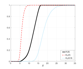
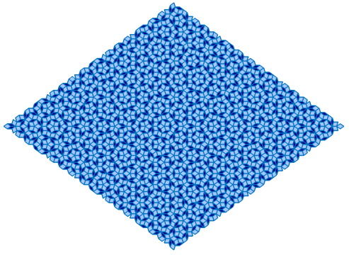
We first give the example of the vertex graph of the Penrose rhomb tiling of the plane (see for example the textbook [3]), shown in Figure 1.
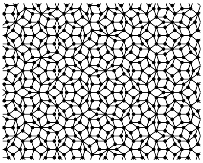
The tiling involves two kinds of rhombuses, a wide rhombus with angles and , and a narrow rhombus with angles and . This Penrose tiling possesses a five-fold rotational symmetry, but is aperiodic, with no translational symmetry. While the vertex graph is also nonregular, it is roughly isometric to (see Section 2.3), so that Theorem 1.1 implies the Landscape Law for Jacobi operators on the Penrose tiling graph .
Next, we consider lattices and some of their variations. Lattices such as the triangular and hexagonal lattices are readily seen to be roughly isometric to . Local perturbations of lattices, such as adding decorations to sites, also remain roughly isometric. Stacked lattices, obtained by taking for a fixed and adding edges between identical sites in adjacent layers, also remain roughly isometric. The landscape law Theorem 1.1 then holds for all these graphs.

1.4. Lifshitz tails for stacked graphs
For a graph , construct the stacked graph as follows, similarly as described for stacked lattices in the previous subsection. The vertices of are , for and , and the edges are those in each copy of ( if in ), along with new edges between identical sites in adjacent copies of , if . This is easiest to visualize when is e.g. a 2D lattice or tiling graph such as in Figure 2.
If the properties in Assumption 2 (defined below in Section 2.2) hold with the natural metric and harmonic weight (2.14) for a graph , then as we verify in Section 5.2, the required properties also hold for the described with metric and “bad set” . Thus if also satisfies the other hypotheses for Theorem 1.2, then this implies that Lifshitz tails for both and the stacked model follow from Corollary 1.3 in this situation.
1.5. Sierpinski gasket graph
We briefly discuss the Sierpinski gasket graph (Figure 3), which is a fractal graph. It is not roughly isometric to any , but it satisfies a similar type of heat kernel bounds, called sub-Gaussian heat kernel bounds (for , one has Gaussian heat kernel bounds). The sub-Gaussian heat kernel bounds allow us to obtain the Landscape Law upper bound Theorem 1.2(ii), for Jacobi operators on the Sierpinski gasket graph. (Section 5.3.)
1.6. Random band models
In this part, we discuss the graph induced by a band matrix on , for which we will see all assumptions required for the Lifshitz tails (1.16) in Corollary 1.3 hold. More precisely, let be a (naturally weighted) graph with the vertex set . For a positive integer , the edge set is defined as follows:
| (1.18) |
where the norm can be the 1-norm (induced by the shortest path metric on ), or the -norm , or the Euclidean-norm , or any other norm which is equivalent to these norms. For , we then write iff . The Jacobi operator in (1.3) is denoted as and acts on functions on as
| (1.19) |
The (negative) Laplacian on , denoted as , is given by setting and in . An example of the graph for , is shown in Figure 4, where the matrix representation of the negative Dirichlet sub-graph Laplacian is
The random operator in matrix form corresponds to adding the potential to the diagonal, and replacing off-diagonal s with the appropriate .
For general and , the band graph is a notable example where all assumptions required in Theorems 1.1 and 1.2 hold. We will prove this later in Section 5.1. As a consequence, we obtain both the landscape law and the Lifshitz tails,
Corollary 1.4 (application to random band matrices).
Lifshitz tails for random band matrices were also proved in [37], using different methods (a variational argument and comparison with a diagonal model).
For other graphs such as the Penrose tiling or Sierpinski gasket graph, we do not have a complete understanding of the geometric properties that would be required to obtain all of the desired results as in Corollary 1.4, though we do obtain some of the results as discussed in previous sections. Instead, in Section 6, we numerically study the landscape law on some of these models, providing strong evidence that the landscape counting functions can be used to establish effective upper and lower bounds for the IDS across various models. Additionally, the numerics demonstrate the advantage of the landscape counting function in productively reflecting the Lifshitz tails through appropriate scalings.
1.7. Outline
The rest of this article is organized as follows.
-
•
In Section 2, we introduce background and preliminaries concerning operators on graphs, the landscape function and landscape counting function, and rough isometries of graphs. We provide precise definitions for all terms and assumptions mentioned for the main results.
- •
- •
- •
-
•
Finally, in Section 6, we provide numerical results for Anderson models on the Penrose tiling and Sierpinski gasket, and for random band models with bond disorders.
Throughout the paper, constants such as , , and may change from line to line. We will use the notation to mean , and to mean , for some constant depending only on . If , we may also write .
2. Preliminaries
In this section, we introduce graph operators and the landscape function, followed by the precise assumptions on the graphs and discussion concerning rough isometries.
2.1. Operators on graphs and the landscape function
For convenience, we collect several useful facts from graph operator theory and landscape function theory in this section. More background and details can be found in [1, §2], [36, §2], and the references therein.
We consider functions on the vertices of the graph, which will be denoted by the function space . We denote by the function which is identically , and by the indicator function of . The space is defined via the norm induced by the usual (non-weighted) inner product The subspaces and are defined accordingly for any finite subset .
The following maximum principle will be useful in obtaining bounds on the landscape function.
Definition 2.
For , we say satisfies the (weak) maximum principle if implies .
Lemma 2.1 (Lemma 2.1, [36]).
Let be a finite subset. If is strictly positive and satisfies the (weak) maximum principle, then for all . As a consequence, the landscape function for all .
The (weak) maximum principle holds widely, including for (and its restriction ) given in (1.3).
Lemma 2.2 (Lemma 2.2, [36]).
Lemma 2.3 (Landscape uncertainty principle).
There is a unique such that . In addition, for ,
| (2.1) |
2.2. Graph properties and assumptions
Roughly speaking, we will want to work on graphs that are amenable to tools from harmonic analysis. This will allow us to adapt tools and methods from [9, 1]. Our first obstruction in moving from or to graphs comes from the non-regular geometry. For the landscape laws in [9, 1], the periodic structure of and was used to construct perfect partitions of cubes and perform arguments utilizing the resulting translation invariance. For graphs, we have no such possibilities and instead must work with coverings rather than partitions, and with certain collections of coverings rather than translation invariance. To this end, we will need certain geometric covering properties. We have the following covering results which are consequences of the volume control assumption (1.1).
Proposition 2.4 (covering properties).
Assume volume control (1.1). Then the following properties hold.
-
(a)
Finite overlap: Then there is a constant such that for any , there is a covering such that
(2.2) -
(b)
Translation replacement: There are constants and so that for any and , there is a collection of at most covers , all with finite covering constant , so that is a covering (not necessarily with any particular covering constant) of .
Proof of Proposition 2.4.
(a) Follows from [7, Lemma 6.2].
(b) First, we can cover a ball with smaller balls , where , using a similar volume comparison argument as in [7, Lemma 6.2]. Take a maximal set of points so that are disjoint, and let be the number of such points. Then covers by maximality, and is a disjoint union contained in the larger ball . Thus
where , so that .
Next, let be a covering with finite overlap constant as in (2.2). For each ball , cover it by the smaller balls as described above (with radius ). We form the covers by taking one center from each . By repeating the elements of , we can ensure there are elements in . Then for , define
which covers since . By construction, covers (even with radii instead). Finally, each has finite overlap covering constant
Example 1.
For the standard lattice, we can consider different balls, such as a cube ( ball), Euclidean ball, or (graph/natural metric) ball, and construct explicit coverings that satisfy Proposition 2.4. For example, the finite overlap property in part (a) is clear for cubes, and follows for the other balls, for example by embedding a cube within each ball and considering a covering with those cubes.
For part (b), we can use the fact that does have translation invariance. Given a cover with finite overlap constant as in (a), consider its translation where is a translation (affine map) mapping the center to . Then for , considering cubes or cubes embedded in the other balls, we only need at most many so that covers for any fixed , and then covers .
Under the finite overlap covering property in (2.3), we prove the following two lemmas, first that one also obtains a finite overlap property for larger balls with the same centers, and second, that the landscape counting function defined in (1.6) is comparable (up to a constant factor) across different choices of coverings .
Lemma 2.5 (Scaled finite overlap covering property).
Proof.
This is a volume comparison. In what follows, will always denote a center of a ball in the given covering . First, the set is the set . Let , which is contained in . By equation (2.2), each point can appear in at most of the balls , so that
Since and , this yields,
∎
If we consider different coverings with similar radii and , the corresponding landscape counting functions differ only by a constant pre-factor depending on . This allows us to work with any specific choice of partition satisfying the finite overlap property (2.2), since the resulting landscape counting functions are equivalent up to the constant factor.
Lemma 2.6 (partition comparison).
Proof.
Next, we discuss several traditional concepts from harmonic analysis that are known to carry over to the discrete setting on graphs.
Definition 3.
The graph satisfies a (weak) Poincaré inequality (PI) if there exist and such that, for all , if and , then
| (2.5) |
where
| (2.6) |
It is well-known that the standard graph satisfies the weak PI (2.5), see e.g. [7, Cor. 3.30]. Note also that by embedding different balls within each other, if the graph satisfies the weak PI with one particular metric for defining the balls, then it also satisfies the weak PI (with possibly different scaling constant ) with any strongly equivalent metric.
Remark 2.1.
In general, one can consider a -Poincaré inequality for any , with the power rather than in (2.5). Under a -Poincaré inequality, if one revises the definition of in (1.6) using covers of radius rather than , then one can still obtain the landscape law upper bound (1.8). We will discuss this further for the Sierpinski gasket graph in Section 5.3.
The weak PI is known to be connected to several other notions concerning random walks and harmonic analysis on graphs. For any , let be the Dirichlet Laplacian on ,
| (2.7) |
and let be the Green’s function on such a ball .
Proposition 2.7.
If satisfies the weak PI (2.5) and volume control (1.1) with parameter , then it also satisfies the following properties.
-
(i)
Moser–Harnack inequality for subharmonic functions: There exists a constant such that for any and non-negative subharmonic function (that is, and ), then
(2.8) -
(ii)
Free landscape/exit time upper bound: There is a positive constant such that for , , and ,
(2.9) (Additionally, by the maximum principle Lemma 2.2, the inequality also holds for the landscape function .)
-
(iii)
Green’s function estimates: For any , let . There are constants depending only on and the ratio , such that
(2.10) -
(iv)
Gaussian heat kernel bounds . (In fact, one has equivalence.) These are defined in terms of the natural graph metric and continuous time heat kernel , where is the continuous time simple random walk on , as
(2.11) for .
Proofs and references for the above results can be found in the textbook [7], particularly Theorems 6.19 and 7.18, and Lemma 4.21. We make two brief remarks concerning the proofs:
-
(1)
First, for property (i), Theorem 7.18 in [7] states the elliptic Harnack inequality (EHI) for harmonic functions. The Moser–Harnack inequality (2.8) for subharmonic functions can be derived from the harmonic version via standard elliptic PDE techniques. We include details for the discrete case in Appendix C for the reader’s convenience.
- (2)
The properties (i)–(iii) in Proposition 2.7 will be utilized in the landscape law proofs. We will see in Section 2.3 that Assumption 1 and the weak Poincaré inequality, which are required for the Landscape Law, will be preserved under rough isometry between graphs. Since the required properties hold for , then the landscape law Theorem 1.1 will hold for all graphs roughly isometric to as well. While these examples have integer values of , Ref. [8] constructed graphs satisfying heat kernel bounds for any real and .
In order to apply the Moser–Harnack inequality in the proof of Theorem 1.1(ii), we will use the following corollary, which uses that the landscape function always satisfies for .
Corollary 2.8 (Moser–Harnack for landscape).
Proof.
In order to obtain the Lifshitz tail upper bound in Theorem 1.2(ii) for , we will also require control on the lower bound of a “harmonic weight” on balls. Most of the time, we work on the natural balls given by the graph or chemical metric (shortest-path distance) on . However, for specific applications, it may be more convenient to consider other distance functions which are (strongly) equivalent to , in the sense that for some universal constants depending only on . We thus state Assumption 2 in terms of a more general metric function, since it may be easier to verify the required properties for a different metric. We will denote by the ball of radius of with respect to the metric , and by the natural metric ball. Immediately, there is so that for any and ,
| (2.13) |
The mean value property of a harmonic function on (on Euclidean balls) states that The integral weight for such an -harmonic function is thus the constant function . A similar mean value property holds for harmonic functions on graphs, but with a general “harmonic weight” function (cf. (2.16)), which also depends on the metric on the graph. In general, the harmonic weight is not unique, and not necessarily a constant (with respect to the volume of the ball), as it is for .
For the natural graph metric , we have , which gives a filtered structure . There is then the following natural way to define a harmonic weight and the volume average on , explicitly through the Poisson kernel or random walk hitting measure on each layer. Letting be a discrete-time simple random walk and the exit time from a region , one can take a harmonic weight for the ball to be
| (2.14) |
This corresponds to values of the Poisson kernel of the ball , normalized by since we will average over layers. More precisely, the Poisson kernel of a region is defined as . For harmonic in with boundary values , , then
| (2.15) |
Thus for harmonic at points in , we have
where the term corresponds to just and . For further background and details, see Appendix A and [27, §6.2], [7, Thm. 2.5].
For a general metric , the boundary of a ball may not relate nicely to larger balls. One can still introduce a harmonic weight in a similar spirit as the above, but which is technically more involved.
We are most interested in the case when there is a harmonic weight that is uniformly bounded from below on most parts of the ball.
Assumption 2.
There is a metric on , strongly equivalent to the natural metric , such that the following hold. Given , , and , there exists a function (the harmonic weight) satisfying
-
•
Submean property: if is -subharmonic in the sense (on a set containing ), then
(2.16) and the equality holds if .
-
•
Uniform lower bound: there is a constant , depending only on , and a ‘bad’ subset such that
(2.17)
From the preceding discussion, we see the continuous analogue of both properties holds immediately on with . In [1], a statement similar to (2.17) was obtained for cubes (-balls), based on explicit formulas of the Green’s function and Poisson kernel on cubes (see Lemma 4.3 of [1]). More generally, for the band graph (1.18), we will prove in Section 5.1 that such a harmonic weight exists with respect to the Euclidean metric on , based on surface area control and Poisson kernel estimates in e.g. [27]. We are curious about such properties on general graphs, in particular:
Question 1.
What properties of a graph guarantee the existence of a harmonic weight such that Assumption 2 holds?
2.3. Rough isometries and properties preserved under them
Here we finally formally define rough isometries between (unweighted) graphs and summarize several key properties preserved under them. We refer readers to [7] for further details.
Definition 4 (rough isometry).
-
•
Let and be metric spaces. A map is a rough isometry if there exists constants such that
If there exists a rough isometry between two spaces then they are roughly isometric, and this is an equivalence relation.
-
•
Let and be connected graphs whose vertices have uniformly bounded degrees. A map is a rough isometry if:
-
(1)
is a rough isometry between the metric spaces and with constants and .
-
(2)
there exists such that for all ,
Two graphs are roughly isometric if there is a rough isometry between them, and this is an equivalence relation.
-
(1)
Example 3.
We revisit the Penrose tiling vertex graph from Section 1.3, which we now view as embedded in with edges of length 1, to provide details demonstrating it is roughly isometric to . Like in [39], which considered another graph derived from the Penrose tiling (the tile graph rather than vertex graph), we start by comparing to for a small . Letting be the map defined by taking to a closest point , we obtain for and sufficiently small (which ensures that is injective),
since and are both of order , while is lower-bounded using the minimum distance between two corners of the rhombi. Then defining via , we obtain for in ,
Additionally, for sufficiently small : One can consider the set of rhombi in the tiling that intersect the straight line segment between and (including intersections on edges and corners). This set allows for a path in between and of length at most twice the cardinality of . The number of such rhombi scales with the length by area considerations (take for example the rectangle around of five units in each direction, which covers ), and so .
Finally, there is a numerical constant (based on the maximum distance between corners of rhombi) so that
As is readily seen, rough isometry preserves bounded geometry (1.2) and (as can be seen with more work) volume control (1.1) (cf. [7, Exercise 4.16]), so that Assumption 1 is preserved under rough isometry. The next proposition states that Proposition 2.4 and the weak Poincaré inequality are also preserved under rough isometry.
Proposition 2.9.
Assume volume control (1.1). The following properties are preserved under rough isometries.
Note that Proposition 2.9(iii) combined with Proposition 2.7 implies that if a graph with volume control satisfies the weak Poincaré inequality, then it and any graph roughly isometric to it also satisfy the Moser–Harnack inequality and exit time upper bound (2.9). For the proofs of Proposition 2.9(iii,iv), see [7, Thms. 3.33, 6.19]. Parts (i) and (ii) follow automatically from Proposition 2.4 since volume control (1.1) is preserved by rough isometry.
3. Proof of the Landscape Law for graphs and random hopping models
In this section, we prove the Landscape Law for graphs and Jacobi/random hopping models as stated in Theorem 1.1. In the upper bound, the main differences from the or case are that we repeatedly use the finite covering property in Proposition 2.4(a) to make up for not having a clean partition into cubes, and that since the bond weights can become arbitrarily close to (or equal to) zero, we must separately truncate and bound these small bond weights using leftover diagonal terms (Lemma 3.1). We must also consider boundary terms coming from inner and outer boundaries of graph balls, as well as the relation to the non-regular shape of , carefully throughout.
In the lower bound, the main difference from or is to utilize Proposition 2.4(b) to make up for not having a clean partition or translation invariance. Combined with Proposition 2.4(a) and scaling in Lemma 2.6, this will allow us to handle comparisons with overlapping covers. Additionally, by allowing for overlapping covers and graph-dependent constants, the proof we give actually provides a simpler proof of the case from [1].
3.1. Proof of the Landscape Law upper bound, Theorem 1.1(i)
Let be the covering radius for the partition, and define the set
so that the landscape landscape counting function (1.6) is .
Case I: We first consider . The other case (large ) corresponds to balls consisting only of a single point, and follows immediately from the landscape uncertainty principle as described in Case II near the end of this subsection.
Let
where is the weighted average of (w.r.t. the natural weight) on and is the degree in the graph , as in the weak PI (2.6). We will show that for , that , so that . For any set , let be the vector with elements for and 0 otherwise. Then the space is the orthogonal complement of . The balls in may not be disjoint, but this does not matter, since we just need an upper bound on . Hence,
and the main work is to bound from below for , which will lead to an upper bound on the number of eigenvalues below an energy in terms of .
In order to obtain a bound like , we consider coordinates in the sum according to whether they are in a ball or in a ball . Coordinates may be in both types of balls, but due to the finite covering property in Proposition 2.4, such overcounting is allowable. We start with balls . In this case, the property implies that
| (3.1) |
where we used the finite covering property (2.3) followed by the landscape uncertainty principle (2.1) for the last two inequalities.
For , we first apply the weak Poincaré inequality (2.5) to with to obtain,
| (3.2) |
where and are given as in (2.5). It remains to bound the right hand side of (3.2) from above by . Note that the kinetic energy term (non-potential term) in the Hamiltonian defined in (1.4) has a weight , which may take the degenerate value zero. If we had for all , then (3.2) is readily bounded using the kinetic term in (1.4) and the finite-overlap property. In the general case where takes values arbitrarily close (or equal to) , we first must truncate the weight and compare the resulting kinetic energy to an additional diagonal term which can be eventually absorbed into . The following truncation lemma allows us to compare the kinetic term in , which may have degenerate weights , to the right hand side of (3.2). The proof of the lemma is given at the end of this section.
Lemma 3.1 (-cutoff).
For and any , let . Then for any region ,
| (3.3) |
As a consequence, by choosing ,
| (3.4) |
Applying the above equation (3.4) to in (3.2), and recalling that , we obtain for ,
| (3.5) |
For showing the right side of (3.5) is bounded by a factor of , one complication is that may contain points outside . This will be handled using the term in as follows. Using that is zero outside and that , we can estimate
| (3.6) |
The diagonal term can be bounded using , and the kinetic term using that by (2.3), for any function on ,
Applying these bounds in (3.6) and summing over then yields
As the latter is exactly , combining with (3.1) and (3.5) then yields
for . Therefore, the number of eigenvalues of below is bounded from above by the codimension of the subspace , that is, for ,
| (3.7) |
By rescaling the energy as , we obtain that for ,
| (3.8) |
3.2. Proof of the Landscape Law lower bound, Theorem 1.1(ii)
Similar to the landscape law upper bound, if we can bound from above by on some subspace , then the eigenvalue counting function at will be at least the dimension of . In what follows, we will consider .
Case I: First we consider for to be determined later. In view of the constants inside the argument of in (1.9), we pre-preemptively take the partition radius . As we will be using the Moser–Harnack inequality (2.12), we will need to work with smaller balls, say of radius for . With the condition , then and .
For a ball , denote by the smaller ball with the same center , and set
First we define a preliminary set as
where denotes a cut-off function supported on defined via
| (3.9) |
Note that for adjacent , that
The functions in need not be orthogonal or linearly independent due to the overlap allowed in the covering. To remedy this, we construct and as follows: To choose a set of disjoint balls from , go through the balls in , and for each ball still remaining, remove all other balls that overlap with . Let be the set of remaining balls. If two balls overlap, then their centers satisfy , and so by the finite cover property (2.3), there can only be balls that overlap . So for each ball we kept for , we only removed at most balls from . Since , then we must have
Now take
Since such have disjoint supports, they are linearly independent and . Additionally, their supports are separated from each other by distance at least , so that for different balls .
Now we want to bound from above for each . First, by the landscape uncertainty principle (2.1) and using that by the definition of , we can bound the numerator as
| (3.10) |
For the denominator, using for which includes , followed by the Moser–Harnack inequality (2.12) yields for ,
| (3.11) |
Using that by the definition of and that , then (3.11) becomes
| (3.12) |
provided that is chosen small enough that .
Combining (3.12) and (3.10) and using then yields
| (3.13) |
Since the for have disjoint supports separated from each other by distance at least , the bound (3.13) holds for all linear combinations , and we obtain
Now to compare favorably to , we will need to make use of Proposition 2.4(b). From this property, there are covers , for , all with a finite covering constant , and such that is also a cover (not necessarily with a particular covering constant), say . Applying the preceding argument to any , we have
| (3.14) |
The negative term is already . For the first term, we apply (3.14) to each cover , , and take the sum, which results in the landscape counting function for the covering with smaller radius . With the summation, we obtain
| (3.15) |
where the term is for any partition with finite overlap constant , and is comparable to . While may not have a particular covering constant, we only need to note that upper bounds (up to the geometric constant in Lemma 2.6).
Case II: . In this case , so that . Retaining the definitions of and from before, then for any in or , we have . If , corresponding to , then the numerator upper bound (3.10) still holds. A lower bound
is immediate, and so using we obtain
which is the same scaling of as in (3.13), leading to the same form as (3.15).
If instead , so that , then we make an adjustment to to ensure the supports are far enough apart. Define as before, and form by going through each ball in , and removing all other balls whose centers are within distance of . By volume control (1.1), there are at most points within distance of , so
Then take Since , the landscape uncertainty principle implies for any ,
which leads to
and a similar lower bound as (3.15), except the bound is for .
Rescaling: With new constants and applying Lemma 2.6 (noting that the constants that arise from having can be taken independent of since ), Cases I and II in summary imply,
Rescaling and using that is (non-strictly) increasing in , we obtain for a constant , that
which completes the proof of Theorem 1.1(ii). ∎
Note that when is small, the above argument requires the domain to contain at least one small ball of radius , leading to the condition . The restrictions on can however be removed easily. If , then . Hence, vanishes for some constant depending only on , leading to . In other words, the landscape law lower bound (1.9) holds (neglecting the negative term on the right hand side) trivially when is small.
4. Lifshitz tails for the landscape counting function
In this section, we prove Theorem 1.2 on Lifshitz tails for the landscape counting function for Jacobi operators on graphs. The process of establishing Lifshitz tails behavior of was done in [9] for and then extended to in [1]. In those settings, only cubes with periodic boundary conditions and diagonal disorder were considered for simplicity. In the current paper, we work on a general domain with Dirichlet boundary conditions and consider both diagonal and off-diagonal disorder. The argument follows the general approach of the and cases, though requires additional consideration for the general graph structure and shape of balls, lack of exact formulas, and metric in Assumption 2. One example where these assumptions are satisfied is the graph induced by a random band model, which we will discuss in Section 5.1.
Recall we are interested in a Jacobi operator of the form (1.3) where and are each sets of i.i.d. random variables, and that such an operator can be written in the form
where
The corresponding quadratic form is
For a finite , the Dirichlet restriction of is
and
| (4.1) |
where .
The Lifshitz tail lower bound proof follows the same method as for or , but accounts for the random hopping terms and uses the “sufficient overlap with balls” property to make up for not having a partition into cubes. The upper bound proof will require more adaptation, in particular dealing with the different metrics in Assumption 2, and the lack of exact formulas for e.g. the Green’s function and Poisson kernel which were utilized in the and cases.
4.1. Lifshitz tails lower bound: proof of Theorem 1.2(i)
For , let for an to be specified later depending only on , and let be a cover of . We will require , i.e. , so that we may later apply volume control (1.1).
From the landscape counting function definition, we have
| (4.2) |
so to prove the lower bound (1.14), we will want to bound from below in terms of the CDF .
Denote by the scaled ball , and let be the discrete cut-off function supported on defined as
Note for , that .
Applying the landscape uncertainty principle (2.1) along with (4.1) implies
| (4.3) |
Since
we then obtain using (4.3), the volume control (1.1), and the condition (1.13) that for and , that
Choosing and using independence of the random variables then yields
Thus with (4.2), we obtain
Since is a covering of , we must have
which completes the proof of (1.14). ∎
4.2. Lifshitz tails upper bound: proof of Theorem 1.2(ii)
For , set for to be determined later (cf. Lemma 4.1), and set be a covering of satisfying (2.3) with a finite overlap constant . Using (4.2), then
| (4.4) |
and so we must bound from above for each . This is achieved by the following lemma.
Lemma 4.1.
Under the assumptions in Theorem 1.2(ii), there is and such that for and any ,
| (4.5) |
Assuming this lemma, we then have
Proof of Theorem 1.2(ii).
The key ingredient to prove Lemma 4.1 is the following deterministic result for the growth of the landscape function .
Lemma 4.2 (landscape growth).
Let be the landscape function for . Choose and with , and let
| (4.6) |
for a constant to be chosen later. Then under the assumptions in Theorem 1.2(ii), for any , there are , , depending only on and , such that if the following two conditions hold for :
-
(i)
there is such that
(4.7) -
(ii)
there is the lower bound on the size of ,
(4.8)
then for , there is such that
| (4.9) |
where with the constant given in (2.13).
One of the key ingredients of the proof of Lemma 4.2 is that the landscape function is superharmonic. We will use submean properties of , together with conditions on in (4.8), to obtain the growth of on a larger ball. Recall that due to Assumption 2, we will work with assumptions on a general metric rather than on the natural metric . Balls with respect to the metric will always be denoted with a superscript, such as or , while balls with respect to the natural metric will either not have the superscript or will be identified with a superscript .
Proof of Lemma 4.2.
Let satisfy as in (4.7). Let the -metric ball and a harmonic weight be given as in Assumption 2, satisfying (2.16) and (2.17).
Before starting with the main cases of the proof, we introduce several useful quantities. We will need to consider weighted averages of the landscape function on balls and spheres, with respect to the metric and the associated harmonic weight . To that end, denote by the weighted surface average of on the exterior boundary ,
where is the Poisson kernel (centered at , with respect to ) defined as in (A.1) on .
Next, denote by the weighted volume average of on , with respect to , defined as
| (4.10) |
One can verify the following by taking a constant function in the integration by parts formula (A.3),
The key properties of and we will need are the following, which follow from submean properties of using that pointwise on :
| (4.11) | ||||
| (4.12) |
- •
- •
Given , we will work on enlarged balls centered at containing (with slightly larger radius under the different metric). In particular, let be the scaling constant between the metric and in (2.13), so that
| (4.13) |
Let be the weighted average of on the -metric ball of radius , as given in the definition (4.10). Then (4.12) yields
Now let be given in (4.6) where will be picked later, and satisfying (4.8). By the conditions for , (4.8), and , we have
| (4.14) |
Let
| (4.15) |
which describes where takes small values, and let
Now we are ready to look for satisfying (4.9) by considering the following two cases:
Case I: . In this case, we have many points where is much smaller than the weighted average . As a consequence, the remaining values must be large to compensate for those in . More precisely, summing over the complement of , the definition of implies
If for some (depends only on and ), then we will be done, since then there is some with . Using (4.12) and with a sufficiently large then implies
provided .
To show we have , first apply Assumption 2 to obtain a and subset such that
| (4.16) |
The lower bound on from (4.14) and of from (4.16) imply for sufficiently large ,
Then it is enough to pick so that (4.9) holds for . Since for , it is clear that .
Case II: . Take for some , which gives . Let and be the surface averages of and the Green’s functions on , with respect to the natural metric (we omit the superscript on the balls for simplicity), respectively. Applying the discrete Green’s identity (integration by parts formula) (A.2) to both and yields
| (4.17) |
With the relation , and defining
| (4.18) |
equation (4.17) then implies
| (4.19) |
We next make two uses of the maximum principle for harmonic functions (see e.g. [36, Lemma 2.2]).
-
•
Since is -harmonic in , the maximum principle implies
with the last inequality because for .
-
•
On the other hand, is -harmonic in and equal to on , so the maximum principle implies for ,
Next, by Proposition 2.7, if , there are the Green’s function bounds
where only depend on and the ratio . Therefore, continuing from (4.19),
| (4.20) |
where in the last line we used that . Recall that by the definition (4.6) of , for all ,
and that by the definition of in (4.15), for all , . Therefore, the last sum in (4.20) can be bounded from below as
where we have now made use of the Case II condition that , and also applied the bound in (4.14). Putting everything together, we thus obtain
provided
Once Lemma 4.2 is established, if , then one can attempt to apply the lemma inductively to construct a sequence of balls with growing radii satisfying (4.9), until one exhausts the region . Because the outcome (4.9) is inputted into the next application of Lemma 4.2, the only remaining condition we need to check each time to apply the lemma is (4.8). The probability that (4.8) holds in each step of the induction can be estimated in terms of the cumulative probability distribution function and , leading to:
Proof of Lemma 4.1.
For , let be the initial scale to be used for Lemma 4.2, and let be a cover of with the finite overlap property (2.3). For any ball , we will bound the probability
| (4.21) |
from above. Considering the event , we will apply Lemma 4.2 repeatedly, assuming (4.8) holds, on each scale , for , until . At this point, the conclusion (4.9) will no longer hold if we start with where obtains its maximum, and so somewhere along the way (for some ), the condition (4.8) must have failed. The gives an upper bound for (4.21) in terms of probabilities of events of the form (4.8), which can in turn be bounded in terms of the CDFs and .
For the first step, we start with the event for some . We suppose the following event also holds
where is defined as in (4.6). Then Lemma 4.2 guarantees a point such that . Note is contained in since
As in the argument in the proof of Proposition 2.4(b), we only need at most many balls of radius to cover , where depends only on the overlap constant in (2.3), and the volume control constants (and ) in (1.1). Then must be located in one of these balls, which we call . We denote by , for the rest of the balls of the same radius that we used to cover . To apply Lemma 4.2 again, we will assume the following event holds,
where are defined as in (4.6) on different balls .
Inductively, suppose we have such that . We can check is contained in since
We only need at most many balls of radius to cover , where again only depends on the overlap constant in (2.3) and volume control constants (and ) in (1.1). Proceeding as before, the new event we need to assume to hold is
where are all the balls of radius that we used to cover .
When we reach the first radius such that with for some , we then consider where the maximum of is attained. Since is the maximum, then . To apply Lemma 4.2, since , we only need many balls to cover the entire domain . The corresponding event we need to assume holds is
Lemma 4.2 then produces a point such that , which contradicts the maximality of . Thus
and
| (4.22) |
Finally, it remains to estimate the probabilities of the events in terms of the CDFs and . For any of the , recall the definition of in (4.6) and rewrite , where
Because counting involves dependent variables, first bound its size in terms of the independent variables ,
Applying the Chernoff bound to the binomial random variables and with the optimal parameter (cf. [1, Lemma 4.5]), there are and such that if and , then
| (4.23) | |||
| (4.24) |
where in the last inequalities we used the lower bound from (1.13) and that . Since , then using independence of the and ,
As the above argument does not depend on the particular center , (4.23), (4.24) and (4.2) hold for all on the different balls . Since there are at most many balls for each , then
| (4.25) |
where for the last inequality we used that are non-decreasing for , and that . Furthermore, implies provided . Combined with the assumption for all , we obtain
Putting all these estimates together with (4.22) and setting with , yields
which proves the landscape Lifshitz tail upper bound (1.15).
Note the above induction starts with the initial scale . For , we can do the following instead: Since by Proposition 2.7(ii), then for (equivalently, ), and the Lifshitz tail upper bound (1.15) holds trivially. For , with constants corresponding to the regime , we can take and jump to the last step directly. Note the here is the one that can be taken in (1.13). Hence, there is no restriction on the diameter of as in the Lifshitz tails lower bound. ∎
As a consequence of Theorem 1.2, we obtain the landscape law for random models in Corollary 1.3. We do not prove Corollary 1.3 directly, as previous work [9, 1] reduced the proof of Corollary 1.3 to the Landscape Law bounds (1.8), (1.9), (1.10) and Lifshitz tail bounds (1.14), (1.15) for . In particular, the landscape law for random models in (1.16) follows from Theorems 1.1 and 1.2 using the argument of [9, Thm. 3.56]. See also [1, §4.2] for an axiomatic version of this method.
5. Details for applications to specific models
In this section, we provide details for applications to random band models (Section 5.1), stacked graphs (Section 5.2), and the Sierpinski gasket graph (Section 5.3).
5.1. Random band model and proof of Corollary 1.4
Recall the standard lattice satisfies Assumption 1 and a (weak) Poincaré inequality (2.5), see e.g. Example 1 and [7]. Retain the definitions of the band graph in (1.18). As mentioned in Example 2 in Section 2.3, is roughly isometric to . As a consequence of Proposition 2.9, all aforementioned properties of will be preserved on by the rough isometry. Hence, Theorem 1.1 can be applied to on since all requirements are met. The (weak) Poincaré inequality (2.5) also guarantees the Lifshitz tails lower bound (1.14) for as long as the domain satisfies (1.13). In order to obtain the Lifshitz tails upper bound (1.15), it remains to explicitly construct a harmonic weight as required in Assumption 2 for . This will then complete the proof of Corollary 1.4.
Denote by the usual Euclidean distance for . For , let be Euclidean ball of radius . Recall on , that iff . The exterior boundary , with respect to this metric, is
Let be the Poisson kernel on in , defined as in (A.4). We will use to construct the desired harmonic weight on the Euclidean ball . Intuitively, we want to define the harmonic weight layer by layer using the Poisson kernel, but the graph structure for complicates the boundary regions. We will thus first need the following technical lemma, which says that “spherical shells” in can be covered by thin layers of exterior boundaries in .
Lemma 5.1.
There is so that for any ,
where , for , and .
We note that if , then , and we do not need the extra thin layers in between. Also note that for , and that
| (5.1) |
We will now use Lemma 5.1 to explicitly construct the harmonic weight and prove Corollary 1.4. The proof of the lemma is left to the end of this section. Let and be as in Lemma 5.1. Then applying Lemma 5.1 several times, for e.g. ,
We rearrange the above radii in increasing order and denote them by , so that , and . The covering can then be rewritten as
We define , which will be the “bad set” in Assumption 2. Note that
| (5.2) |
for some constant depending only on , so that as . Overall, Lemma 5.1 thus allows us to cover a large portion of using thin exterior boundaries of Euclidean balls. With such a filtration, we can define the associated harmonic weight on layer by layer.
For , we then set
| (5.3) |
and for , set .
We first verify that is a harmonic weight satisfying (2.16) from Assumption 2. Suppose (for ). Then by the surface submean property (A.5), for any ,
Multiply the equation both sides by the volume (cardinality) of and then sum all the equations from to (setting ) to obtain
which implies
where is given as in (5.3). Putting together the definition for , one concludes that for ,
which verifies (2.16). Clearly, the equality holds if is harmonic ().
We already verified the ‘bad’ set is small in (5.2). It thus remains to show that has the desired lower bound in (2.17) on . For this, we will need the following Poisson kernel bounds.
Proposition 5.2 (Lemma 6.3.7 in [27]).
There are constants depending only on such that
| (5.4) |
From classical results, as the standard Euclidean ball contains lattice points, where is the volume of the unit Euclidean ball in ; see e.g. [41, 17, 20] for further references and more precise error estimates. Thus there is so that for a fixed and all ,
Using this lower bound between the layers in (5.1), we have
Combined with the lower bound in (5.4), this implies for ,
Since for , the sum (5.3) contains at least one (non-zero) term. Hence,
Proof of Lemma 5.1.
Since the annulus is symmetric and -translation invariant, it is enough to consider where , and . In this region, satisfies
Since is the maximal direction, consider the point , which is a neighbor in . We will see that if is relatively large (compared to ), then so that . Otherwise, we will need intermediate layers of thickness to reach the entire annulus. Direct computation using and shows
Hence, if , then for , , so that and .
If , set
For each , if , then and imply
for . This shows , hence since .
The above works for all . In the last layer when , we have
and similarly as before,
provided , where . Hence, and , where we set . ∎
5.2. Stacked graphs
In this section, we provide details for the application to stacks of graphs in Section 1.4. In particular, we verify that if Assumption 2 holds for a graph with the natural metric , then the required properties also hold for the stacked graph with the metric . Since the weak Poincaré inequality is preserved under rough isometry, this together allows for obtaining Lifshitz tails for via Corollary 1.3.
First, the metric is strongly equivalent to the natural metric on . The balls under the metric are simpler however. For , the ball is . For , the ball centered at is the singleton set .
To define the harmonic weight , we use the random walk formulation of the Poisson kernel for the ball . Letting be the Poisson kernel for a region , we will take
| (5.5) |
We can then check the required properties in Assumption 2.
-
•
Submean property: For and harmonic at points in , then for any , the Poisson kernel property (2.15) implies
(5.6) Averaging over , then
(5.7) The required inequality (2.16) then follows for subharmonic functions from (5.6). If then we can simply take the “trivial” harmonic weight , since the second property in Assumption 2 only matters as .
-
•
Bad set: The plan is to compare for to the harmonic weight for , using the random walk relation and Laplace equation properties of the Poisson kernel. We claim that if is the “bad set” for in , then can be taken as the “bad set” for .
Since we added the entire stack of points to the bad set, we can ignore it and only consider the Poisson kernel at points and with , i.e. . Assuming , we first show that for ,
are all comparable. For a path of length exiting at , we can construct a path of length exiting at instead, by following up to and then moving vertically to the th layer before exiting. Since the maximum degree in is bounded by , this implies
(5.8) for any .
Averaging (5.8) over yields for ,
(5.9) where is simple random walk on . The last equality follows using the Poisson kernel formula for solving Laplace’s equation: For a finite region , let be the Poisson kernel on and be the Poisson kernel on . If is harmonic on with boundary values for , then defined as is also harmonic on with boundary values for . Then
and also
By considering boundary values , this implies we must have
(5.10) Taking yields (• ‣ 5.2).
5.3. Sierpinski gasket graph
In this part, we discuss the landscape law and Lifshitz tails for Jacobi operators on the Sierpinski gasket graph , drawn in Figure 3. The Sierpinski gasket graph is a fractal-like graph, and is not roughly isometric to any . Let be the unit triangle on with vertices . Then is constructed using the images of (as vertices) by the iteration of . Let be the set of vertices of the triangles of side length 1 in . Let . The edge set is defined by the relation iff belongs to a triangle in for some . The Sierpinski gasket graph is then .
A key feature of is that it satisfies sub-Gaussian heat kernel bound ; for ,
where is the (continuous time) heat kernel as in (2.11), is the volume growth parameter as in (1.1), and is the sub-Gaussian parameter. (See e.g. [7, Cor. 6.11].) Since the volume control property (1.1) holds, we have the covering of balls provided by Proposition 2.4. As mentioned in Remark 2.1, the parameter is equivalent to the parameter used in (weak) Poincaré inequalities. In the previous sections of this paper, we focused on the case and assumed the corresponding weak Poincaré inequality (2.5). On , as a result of the sub-Gaussian heat kernel bounds, a -version of (2.5) holds [7, §6], with rather than in the Poincaré inequality, i.e.,
with the same average , and the ball scaling as in . This suggests to consider a slightly different landscape counting function , which depends on the parameter . More precisely, unlike coverings of radius used in (1.7), instead, we consider coverings of radius . The associated landscape counting function is defined as
| (5.11) |
Following the proof in Section 3.1, replacing the use of Poincaré inequality (2.5) by its -version, one can obtain the landscape law upper bound
| (5.12) |
where depends on .
Unfortunately, the argument for the landscape lower bounds (1.9), (1.10) does not go through for . Additionally, we do not verify Assumption 2 for the gasket graph, which prevents using the landscape law argument to obtain a version of the Lifshitz tails property.
Recently, authors in [6] established the Lifshitz tails singularity of the integrated density of states for certain random operators on (continuous) nested fractals, including the continuous Anderson model on the planar Sierpinski gasket set; see also earlier related work in [32, 35, 22]. In particular, for (infinite volume) IDS of a random Schrödinger operator (under mild condition on the hopping and the random distribution) on the planar Sierpinski gasket set, Ref. [6] showed that
| (5.13) |
6. Numerical cases
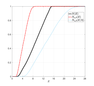
In this section, we introduce and discuss a series of detailed numerical simulations aimed at investigating the behavior of the landscape counting function . These simulations identify more precise behavior (such as explicit numerically determined scalings) governed by our general results Theorems 1.1 and 1.2, and also provide evidence for a landscape law or Lifshitz tails in models where we lack an analytical proof. To comprehensively explore the applicability of the landscape law, we will consider a variety of cases, including random band models, and the Anderson model on the Sierpinski gasket graph and Penrose tiling.
6.1. Random band models
Let’s first recall some of the notations to be used in this section. Let be the graph defined in Section 1.6, where the vertex set is and the edge set has the “-step band structure” in (1.18). Our results in Section 1.6 apply to Jacobi operators (1.19) with both onsite and bond disorders. In the numerical simulations, we will focus only on the bond disorder, i.e., operators in the form
We will consider the above operator in the cases (see in Figure 4 and in Figure 5) for different choices of bandwidth . For the cases, the graph is induced by a band matrix on . Specifically, we employ the -norm to define . As a point of comparison with Figure 4, Figure 5 provides an illustrative example that displays all nodes connected to the central node within a bandwidth of .
In Figure 6, the top row shows an example in 1D with and , where the bond interactions will be modeled using a uniform distribution over the interval [0,1]. The bottom row shows a 2D example using a Bernoulli distribution taking values in {0,1} with half and half probabilities, where and . Furthermore, the on-site non-negative potential is set to be 0. It is important to note that the simulations presented are based on a single random realization, rather than on the average of multiple realizations.
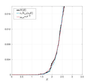
Building upon the previously discussed configurations, we globally get the control of the IDS from above and below through the landscape counting functions. Besides, beyond the global bounds from above and below, the landscape counting function, upon appropriate scaling, can serve as a good approximation for the Lifshitz tail of the IDS. The examples shown in Figure 6(b) and (e) are also to show how the suitably scaled landscape counting function closely mirrors the behavior of the Lifshitz tail (1.21) under varying conditions:
6.2. Sierpinski gasket
Next, we consider the Anderson model (without the bond disorder)
on Sierpinski gasket graph discussed in Section 5.3 (see Figure 3, a fractal structure composed of interconnected equilateral triangles). For the landscape counting function, we specifically employ equilateral triangular boxes for the counting process. Figure 7 illustrates one such example, demonstrating the methodology employed to compute the landscape counting function in (5.11).
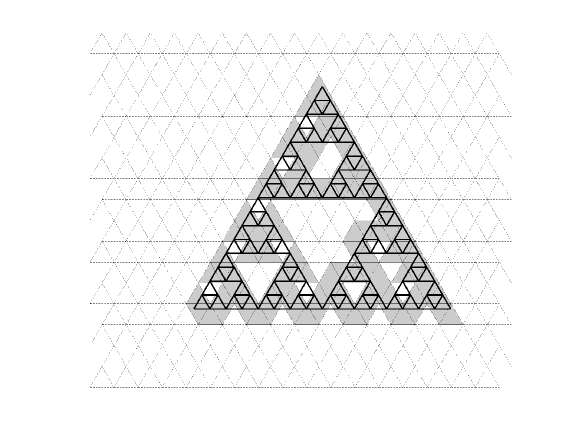
Given that the Sierpinski gasket possesses a volume growth parameter , we define the box size using , where . As discussed in Section 5.3, we are only able to prove the landscape law upper bound (5.12) on the Sierpinski gasket. We expect a landscape law lower bound should also hold. We will next illustrate the application of the landscape law. Note that in this example, we consider only the on-site non-negative potential , without implementing any bond interaction. The subsequent figure presents the landscape law, with selected uniformly at random between 0 and 10, and .
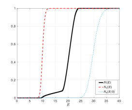
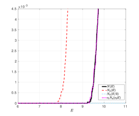
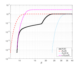
6.3. Penrose tiling
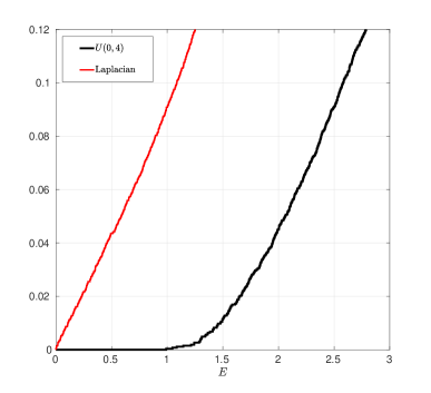
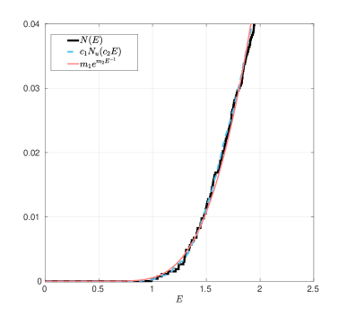
Lastly, we present an example illustrating the Lifshitz tail for the Anderson model on the Penrose tiling in Section 1.3 (see Figure 1), employing Neumann boundary conditions. The on-site non-negative potential is randomly assigned values from a uniform distribution . As discussed in Example 3, the Penrose tiling is roughly isometric to . Hence, Theorem 1.1 can be applied to the Anderson model on it with . As we do not verify the harmonic weight assumption in Assumption 2 for the Penrose tiling, we do not obtain the Lifshitz tails results through Corollary 1.3, though here we provide numerical evidence supporting the behavior. In Figure 9(c), we display the low energy regime of the IDS, fitted by an exponential function. Additionally, a scaled landscape counting function is presented, which is calculated over the lattice of equilateral triangles as illustrated in Figure 7. For comparative purposes, we also calculate the IDS for the free Laplacian over the same tiling in Figure 9(b).
Appendix A Green’s function and Poisson kernel for a Dirichlet Laplacian on a ball
We summarize some facts about Green’s function and Poisson kernel on graphs. These are standard results and can be found in e.g. [7, 27].
Let be a graph, equipped with some distance function . Note that this distance function and the results in this section are not limited to the natural graph metric (shortest-path distance). The graph Laplacian is
For a ball , the Dirichlet Laplacian on is:
The exterior boundary of is and the interior boundary is defined as . Denote by the discrete closure of . Let be the Green’s function associated with . And denote by the associated Poisson kernel. Recall that and are the unique solutions to the following systems: for any ,
and for any ,
| (A.1) |
One can verify the following integration by parts formula for supported on and any ,
By taking , then we see
| (A.2) | ||||
| (A.3) |
where the second line follows from the relation between the Green’s function and the associated Poisson’s kernel
| (A.4) |
Appendix B An explicit proof of Poisson kernel estimates for the 1D random band model
To obtain the general Lifshitz tails lower bound, one needs the control on the Poisson kernel as in Proposition 5.2, which provides the harmonic weight as required by Assumption 2. One notable example where we have such estimates is the graph (1.18) induced by the band model.
The above general case is obtained in [27] by the method of random walk. Below, we give a direct proof of the case with explicit constants depending on the band width . Recall on , . The associated graph Laplacian is
In this part, we use the natural graph metric (shortest path) . Then the ball centered at of radius is , with exterior boundary , and interior boundary . (For 1D, it is enough to consider integer valued radius only.) We denote by and the Green’s function and the Poisson’s kernel of on , respectively.
Lemma B.1.
For all ,
| (B.1) |
For all ,
| (B.2) |
Proof of (B.1).
Without loss of generality, we assume and only consider . The following estimates hold for any center by translation. It is clear that with , and with and .
Notice that . Let be the centric (0th) column of . Since is the inverse of , then . To estimate from above, we choose a test function
for any . Direct computation shows that
Hence, for all . By the maximum principle of , one obtains for all . In particular, for ,
| (B.3) |
Next, we get a lower bound of through the test function
Direct computation shows
leading to for all . By the maximum principle again, for all . In particular, for , one has
Together with (B.3), we have that for ,
| (B.4) |
Recall the relation between and in (A.4),
Clearly, for , . As a consequence of (B.4),
which completes the proof of (B.2). ∎
Notice in this 1D model with the natural metric , for all . To construct the harmonic weight, we do not need the filtration lemma Claim 5.1. One can define directly
Appendix C Moser–Harnack inequality for subharmonic functions
We say a graph satisfies an elliptic Harnack inequality (EHI), given ,, and , if there exists a constant depending only on and , such that for on and harmonic () in , then
| (C.1) |
Under the volume control assumption (1.1), EHI is equivalent to the (weak) Poincaré inequality (2.5) or the Gaussian heat kernel estimates (2.11); for more discussion see the textbook [7], particularly Theorems 6.19 and 7.18, and Lemma 4.21.
Clearly, (EHI) implies the Moser–Harnack inequality
| (C.2) |
for a positive harmonic function and any scaling constant . The version (2.8) that we need for a subharmonic function essentially follows from the harmonic version, combined with the discrete Caccioppoli (“reverse Poincaré”) inequality and Poincaré inequality with Dirichlet boundary conditions. The authors in [28] proved a Moser–Harnack inequality for subharmonic functions on general graphs without the volume control assumptions (1.1), where the Moser–Harnack constant depends exponentially large on the radius of the ball. We did not find a radius-independent version of [28, Theorem 1.2] in the literature, and so we sketch the proof of (2.8) here for completeness.
Throughout, we write for a ball centered at of radius . Let be a finite set. Define the Dirichlet energy subject to the boundary condition on to be
| (C.3) |
Note that in some literature, the concept ‘Dirichlet form’ may refer to the energy with the zero boundary condition on , see e.g. [7, §1.4], that is:
The equality holds only if on the exterior boundary .
The following is the discrete version of the well-known energy minimizing property of a harmonic function.
Lemma C.1 (Energy minimizer, [18, Theorem 3.5]).
If is harmonic on , then is a minimizer of among functions in with the same values on . More precisely, if , then for any satisfying on ,
| (C.4) |
Lemma C.2 (discrete Caccioppoli inequality, see e.g. [28, Lemma 2.4]).
Let , and . Suppose is a nonnegative and subharmonic function on . Then we have
| (C.5) |
where depends only on and from (1.2).
This follows the proof of the Caccioppoli inequality for functions on , see e.g. [15, §4.1].
Proof.
Let the cut-off function constructed (in a similar manner) as in (3.9), satisfying on , for , and for all .
Since for , then for the test function , the discrete Gauss–Green Theorem (integration by parts, see e.g. [7, Theorem 1.24]) implies
| (C.6) |
where we used that Therefore (C.6), with Cauchy–Schwarz and properties of , implies
Dividing both sides by the square root of the left hand side, and using that on , yields
| (C.7) |
∎
Next, we will need that the weak (or “mean”) Poincaré inequality (2.5) implies the following zero-boundary Poincaré inequality. We do not actually directly use the weak PI formulation (2.5), but just that the exit time bound in Proposition 2.7(ii) holds.
Lemma C.3 (Poincaré inequality with the Dirichlet boundary condition).
Proof.
Let and be the Dirichlet Laplacian on . Let be the smallest eigenvalue of . By Proposition 2.7(ii), there is the bound . Since in general (see e.g. [36, Lemma 2.1]), then for some depending only on ,
Notice that when on , the Dirichlet energy in (C.3) equals the Dirichlet energy subject to the zero boundary condition:
Then (C.8) follows directly from the definition of the ground state energy by minimizing the zero-boundary Dirichlet energy (among functions not identically zero) on the right hand side. ∎
Proof of (2.8).
The idea follows from the outline of the proof of [28, Theorem 1.2]. However, we must consider the (in)dependence of the radius more carefully using (C.5) and (C.8). Let be a subharmonic function on . Let be a harmonic function on on which agrees on the (exterior) boundary of , i.e., satisfies and for . By the maximum principle, on . Then the Moser–Harnack property (C.2) (with ) for implies
| (C.9) |
The second term is readily bounded by a constant times the average of on using the volume control (1.1). For the first sum, since on , by the Poincaré inequality (C.8),
| (C.10) |
where in the last line we used (C.4), that the harmonic function is a minimizer of the energy . Then the Caccioppoli inequality (C.5) implies the sum in (C.10) is bounded as
leading to for some constant independent of . Using this in (C.9), we obtain
∎
Acknowledgments. The authors would like to thank Douglas N. Arnold and Svitlana Mayboroda for useful discussions. L.S. was supported in part by the Julian Schwinger Foundation for Physics Research and Simons Foundation grant 563916, SM.
References
- [1] D. Arnold, M. Filoche, S. Mayboroda, W. Wang, and S. Zhang. The landscape law for tight binding Hamiltonians. Communications in Mathematical Physics, 396(3):1339–1391, 2022.
- [2] D. N. Arnold, G. David, M. Filoche, D. Jerison, and S. Mayboroda. Computing spectra without solving eigenvalue problems. SIAM Journal on Scientific Computing, 41(1):B69–B92, 2019.
- [3] M. Baake and U. Grimm. Aperiodic order. Vol. 1, volume 149 of Encyclopedia of Mathematics and its Applications. Cambridge University Press, Cambridge, 2013. A mathematical invitation, With a foreword by Roger Penrose.
- [4] S. Bachmann, R. Froese, and S. Schraven. Counting eigenvalues of Schrödinger operators using the landscape function. J. Spectr. Theory, 13(4):1445–1472, 2023.
- [5] S. Bachmann, R. Froese, and S. Schraven. Two-sided Lieb-Thirring bounds. arXiv preprint arXiv:2403.19023, 2024.
- [6] H. Balsam, K. Kaleta, M. Olszewski, and K. Pietruska-Pałuba. Density of states for the Anderson model on nested fractals. arXiv preprint arXiv:2303.05980, 2023.
- [7] M. Barlow. Random Walks and Heat Kernels on Graphs. Number 438 in London Mathematical Society Lecture Note Series. Cambridge University Press, 2017.
- [8] M. T. Barlow. Which values of the volume growth and escape time exponent are possible for a graph? Rev. Mat. Iberoamericana, 20(1):1–31, 2004.
- [9] G. David, M. Filoche, and S. Mayboroda. The landscape law for the integrated density of states. Advances in Mathematics, 390:107946, 2021.
- [10] P. Desforges, S. Mayboroda, S. Zhang, G. David, D. N. Arnold, W. Wang, and M. Filoche. Sharp estimates for the integrated density of states in Anderson tight-binding models. Physical Review A, 104(1):012207, 2021.
- [11] F. J. Dyson. The dynamics of a disordered linear chain. Phys. Rev., 92:1331–1338, Dec 1953.
- [12] C. L. Fefferman. The uncertainty principle. Bull. Amer. Math. Soc. (N.S.), 9(2):129–206, 1983.
- [13] A. Figotin and A. Klein. Localization of electromagnetic and acoustic waves in random media. Lattice models. J. Statist. Phys., 76(3-4):985–1003, 1994.
- [14] M. Filoche and S. Mayboroda. Universal mechanism for Anderson and weak localization. Proceedings of the National Academy of Sciences, 109(37):14761–14766, 2012.
- [15] M. Giaquinta and L. Martinazzi. An introduction to the regularity theory for elliptic systems, harmonic maps and minimal graphs, volume 11 of Appunti. Scuola Normale Superiore di Pisa (Nuova Serie) [Lecture Notes. Scuola Normale Superiore di Pisa (New Series)]. Edizioni della Normale, Pisa, second edition, 2012.
- [16] M. Gromov. Hyperbolic groups. In Essays in group theory, volume 8 of Math. Sci. Res. Inst. Publ., pages 75–263. Springer, New York, 1987.
- [17] D. R. Heath-Brown. Lattice points in the sphere. In Number theory in progress, Vol. 2 (Zakopane-Kościelisko, 1997), pages 883–892. de Gruyter, Berlin, 1999.
- [18] I. Holopainen and P. M. Soardi. -harmonic functions on graphs and manifolds. Manuscripta Math., 94(1):95–110, 1997.
- [19] J. G. Hoskins, H. Quan, and S. Steinerberger. Magnetic Schrödinger operators and landscape functions. Comm. Partial Differential Equations, 49(1-2):1–14, 2024.
- [20] M. N. Huxley. Exponential sums and lattice points. III. Proc. London Math. Soc. (3), 87(3):591–609, 2003.
- [21] M. Inui, S. A. Trugman, and E. Abrahams. Unusual properties of midband states in systems with off-diagonal disorder. Phys. Rev. B, 49:3190–3196, Feb 1994.
- [22] K. Kaleta and K. Pietruska-Pałuba. Integrated density of states for Poisson–Schrödinger perturbations of subordinate Brownian motions on the Sierpiński gasket. Stochastic Processes and their Applications, 125(4):1244–1281, 2015.
- [23] W. Kirsch. An invitation to random Schrödinger operators. In Random Schrödinger operators, volume 25 of Panor. Synthèses, pages 1–119. Soc. Math. France, Paris, 2008. With an appendix by Frédéric Klopp.
- [24] W. Kirsch and P. Müller. Spectral properties of the Laplacian on bond-percolation graphs. Math. Z., 252(4):899–916, 2006.
- [25] F. Klopp and S. Nakamura. A note on Anderson localization for the random hopping model. J. Math. Phys., 44(11):4975–4980, 2003.
- [26] W. König. The parabolic Anderson model. Pathways in Mathematics. Birkhäuser/Springer, [Cham], 2016. Random walk in random potential.
- [27] G. F. Lawler and V. Limic. Random walk: a modern introduction, volume 123. Cambridge University Press, 2010.
- [28] Y. Lin and H. Song. Harnack and mean value inequalities on graphs. Acta Math. Sci. Ser. B (Engl. Ed.), 38(6):1751–1758, 2018.
- [29] J. Lu, C. Murphey, and S. Steinerberger. Fast localization of eigenfunctions via smoothed potentials. J. Sci. Comput., 90(1):Paper No. 38, 18, 2022.
- [30] P. Müller and P. Stollmann. Spectral asymptotics of the Laplacian on super-critical bond-percolation graphs. J. Funct. Anal., 252:233–246, 2007.
- [31] P. Müller and P. Stollmann. Percolation Hamiltonians. In Random walks, boundaries and spectra, volume 64 of Progr. Probab., pages 235–258. Birkhäuser/Springer Basel AG, Basel, 2011.
- [32] K. Pietruska-Paluba. The Lifschitz singularity for the density of states on the Sierpinski gasket. Probability theory and related fields, 89(1):1–33, 1991.
- [33] B. Poggi. Applications of the landscape function for Schrödinger operators with singular potentials and irregular magnetic fields. Adv. Math., 445:Paper No. 109665, 54, 2024.
- [34] D. Sánchez-Mendoza. Principal eigenvalue and landscape function of the Anderson model on a large box. J. Stat. Phys., 190(7):Paper No. 122, 19, 2023.
- [35] T. Shima. Lifschitz tails for random Schrödinger operators on nested fractals. Osaka J. Math., 29(4):749–770, 1992.
- [36] L. Shou, W. Wang, and S. Zhang. Landscape approximation of the ground state eigenvalue for graphs and random hopping models. Journal of Functional Analysis, 286(7):110339, 2024.
- [37] B. Staffler. Lifshitz tails for random band matrices. Master’s thesis, LMU Munich, Theoretical and Mathematical Physics, 2013.
- [38] S. Steinerberger. An Agmon estimate for Schrödinger operators on graphs. Lett. Math. Phys., 113(1):Paper No. 12, 9, 2023.
- [39] A. Telcs. Diffusive limits on the Penrose tiling. J. Stat. Phys., 141(4):661–668, 2010.
- [40] G. Theodorou and M. H. Cohen. Extended states in a one-demensional system with off-diagonal disorder. Phys. Rev. B, 13:4597–4601, May 1976.
- [41] A. Walfisz. Gitterpunkte in mehrdimensionalen Kugeln. Jber. Deutsch. Math.-Verein., 61:11–31, 1958.
————————————–
L. Shou, Condensed Matter Theory Center and Joint Quantum Institute, Department of Physics, University of Maryland, College Park, MD 20742, USA
E-mail address: lshou@umd.edu
W. Wang, LSEC, Institute of Computational Mathematics and Scientific/Engineering Computing, Academy of Mathematics and Systems Science, Chinese Academy of Sciences, Beijing 100190, China
E-mail address: ww@lsec.cc.ac.cn
S. Zhang, Department of Mathematics and Statistics, University of Massachusetts Lowell, Southwick Hall, 11 University Ave. Lowell, MA 01854
E-mail address: shiwen_zhang@uml.edu