figurec
Scaling Continuous Latent Variable Models as Probabilistic Integral Circuits
Abstract
Probabilistic integral circuits (PICs) have been recently introduced as probabilistic models enjoying the key ingredient behind expressive generative models: continuous latent variables (LVs). PICs are symbolic computational graphs defining continuous LV models as hierarchies of functions that are summed and multiplied together, or integrated over some LVs. They are tractable if LVs can be analytically integrated out, otherwise they can be approximated by tractable probabilistic circuits (PC) encoding a hierarchical numerical quadrature process, called QPCs.
So far, only tree-shaped PICs have been explored, and training them via numerical quadrature requires memory-intensive processing at scale. In this paper, we address these issues, and present: (i) a pipeline for building DAG-shaped PICs out of arbitrary variable decompositions, (ii) a procedure for training PICs using tensorized circuit architectures, and (iii) neural functional sharing techniques to allow scalable training. In extensive experiments, we showcase the effectiveness of functional sharing and the superiority of QPCs over traditional PCs.
1 Introduction
Continuous latent variables (LVs) are arguably the key ingredient behind many successful generative models, from variational autoencoders [24] to generative adversarial networks [20], and more recently diffusion models [56]. While these models allow to learn expressive distributions from data, they are limited to sampling and require task-specific approximations when it comes to perform probabilistic reasoning, as even simple tasks such as computing marginals or conditionals are intractable for them. On the other hand, performing these tasks can be tractable for (hierarchical) discrete LV models [4, 3], but these prove to be more challenging to learn at scale [9, 10, 32, 33].
This inherent trade-off among tractability, ease of learning, and expressiveness can be analyzed and explored with probabilistic integral circuits (PICs) [18], a recently introduced class of deep generative models defining hierarchies of continuous LVs using symbolic functional circuits. PICs are tractable when their continuous LVs can be analytically integrated out. Intractable PICs can however be systematically approximated as (tensorized) probabilistic circuits (PCs) [53, 4], the representation language of discrete LV models. An instance of such PCs encodes a hierarchical numerical quadrature process of the PIC to approximate, and as such is called quadrature PC (QPC).
Distilling QPCs from PICs has proven to be an effective alternative way to train PCs, but it has only been explored for tree-shaped PICs, as building and scaling to richer LV structures is an open research question that requires new tools [18]. In this paper, we fill this gap by redefining the semantics of PICs and extending them to DAG-shaped hierarchies of continuous LVs. Specifically, we design PICs as a language to represent hierarchical quasi-tensors factorizations [49], parameterized by light-weight multi-layer perceptrons.
Contributions.
(1) We present a systematic pipeline to build DAG-shaped PICs, starting from arbitrary variable decompositions (Section 3.1). (2) We show how to learn and approximate PICs via a hierarchical quadrature process which we encode in tensorized QPCs that match certain circuit architectures proposed in different prior works [43, 42, 31, 39] (Section 3.2). (3) We present functional sharing techniques to scale the training of PICs, which lead us to parameterize them with multi-headed multi-layer perceptrons (MLPs) requiring comparable resources as PCs (Section 3.3). (4) In extensive experiments (Section 4), we show that (i) functional sharing proves remarkably effective for scaling and that (ii) QPCs outperform PCs commonly trained via EM or SGD, while being distilled from PICs with up to 99% less trainable parameters.
2 Probabilistic integral circuits
Notation
We denote input variables as and latent variables (LVs) as and , with and as their realization respectively. We denote scalars with lower-case letters (e.g., ), vectors with boldface lower-case letters (e.g., ), matrices with boldface upper-case letters (excluding , e.g., ), and tensors with boldface calligraphic letters (e.g., ).
A probabilistic integral circuit (PIC) is a symbolic computational graph representing a function over observed variables and continuous latent variables . Similar to probabilistic circuits (PCs) [53, 4], PICs have input, sum and product units.111We refer the reader to Appendix A for an introductory overview of (probabilistic) circuits. Different from PCs, however, PICs operate on functions, not scalars, and make use of a new type of unit: the integral unit.
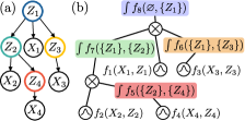
More formally, an input unit (depicted as in our figures) represents a possibly unnormalized distribution , where and . A sum unit () outputs a weighted sum of its input functions, i.e. , where and and and, similarly, a product unit () outputs the product of its input functions, i.e. . Finally, an integral unit () encodes an “uncountable weighted sum” whose weights are compactly represented by a function , where are the LVs that are being integrated out by . The unit receives a function from its only input unit and outputs the function . Fig. 1(b) and Fig. 2(b) show example PICs.
Similar to PCs, imposing structural constraints over PICs can unlock tractable inference [4]. As such, we assume that (i) all -units receive functions defined on the same input variables (aka smoothness), and (ii) all -units receive functions defined over disjoint sets of input variables (aka decomposability). We also assume that every -unit integrates out all incoming LVs, potentially introducing new ones, i.e. computes . In this way, the output LVs of any unit will simply be .
PICs are tractable when their LVs can be analytically integrated out, meaning that we can pass-through integral units computing the integration problem they define, eventually outputting a function. Notably, this is possible when LVs are in linear-Gaussian relationships [27] or when functions are polynomials. Intractable PICs can however be approximated via a hierarchical numerical quadrature process that can be encoded as a PC called quadrature PC (QPC). Intuitively, each PIC integral unit can be approximated by a set of sum units in a QPC, each conditioning on some previously computed quadrature values, with a large but finite number of input units [18]. Materializing a QPC allows to train PICs by approximate maximum likelihood: Given a PIC, gradients to its parameters attached to input, sum and integral units can be backpropagated through the corresponding QPC [18]. This also provides an alternative way to train PCs that can rival traditional learners.
So far, the construction of PICs has been limited to a compilation process from probabilistic graphical models (PGMs) [27] with continuous LVs [18]. In a nutshell, the LV nodes of a PGM become integral units in a PIC, and the PGM conditional distributions become the input and integral functions of the PIC, as illustrated in Fig. 1. However, the PGM structure needs to be limited to a tree, as to avoid that the hierarchical quadrature process would yield an exponentially large QPC, thus hindering learning. This imposes a semantics for current PICs as latent tree models [3], and clearly limits their expressiveness as more complex LV interactions are not possible. Building more expressive PICs requires reinterpreting this semantics and introducing new tools, which we do next.
3 Building, learning and scaling PICs
In Section 3.1, we systematize the construction of DAG-shaped PICs, showing how to build them starting from arbitrary variable decompositions, going beyond the current state-of-the-art [18]. Then, in Section 3.2, we show how to learn and approximate such PICs with QPCs encoding a hierarchical quadrature process, retrieving PC architectures proposed in prior works [39]. Finally, in Section 3.3, we present (neural) functional sharing, a technique which we use to parameterize PICs as to make their QPC materialization fast and cheap, allowing scaling to larger models and larger datasets.
3.1 Building PICs from arbitrary variable decompositions
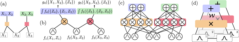
Standard PCs can be built according to established pipelines that allow to flexibly represent arbitrary variable decompositions, as well as rich discrete LV interactions [39, 41]. In the following, we derive an analogous pipeline for PICs that allows to take care of continuous LVs, going beyond their current tree-shaped semantics (Section 2) yet allowing to perform hierarchical quadrature without blowing up the size of the materialized QPCs. To do so, we start by formalizing the notion of hierarchical variable decomposition, or region graph, out of which we will build our PIC structures.
Definition 1 (Region Graph (RG) [15]).
An RG over input variables is a bipartite and rooted directed acyclic graph (DAG) whose nodes are either regions, denoting subsets of , or partitions, specifying how a region is partitioned into other regions (Fig. 2(a)).
RGs can be (i) compiled from PGMs [5, 27, 3, 31], (ii) randomly initialized [43, 16], (iii) learned from data [15, 19, 40, 57], or (iv) built according to the data modality (e.g. images) [45, 42, 39]. If we compile from a tree PGM, as in (Fig. 1), the resulting RG will be a tree, thus yielding a tree-like PIC [18]. Our pipeline, detailed in Algorithm 1, takes an arbitrary DAG-shaped RG as input, and can deliver DAG-like PICs. Without loss of generality, we assume to have an RG which only allows for (i) binary partitionings of regions (i.e. all product units will have two input units) and (ii) univariate leaves, as shown in Fig. 2(a). Our construction iteratively builds a PIC in a bottom-up fashion, associating regions to PIC units. For every leaf region in , we instantiate an input unit with function , where is an arbitrary continuous LV (8, Algorithm 1). Such functions can be univariate conditional densities, i.e. , resembling small VAE-like decoders [24] amenable to be numerically integrated.
Once all leaf regions have been processed, we move to the inner ones. Let be an inner region partitioned in different ways as , i.e. and for every . For each partition , we will merge the PIC units associated to regions and using consecutive applications of product and integral units—as we explain next—eventually associating a unit the partition itself. One can design such merging as desired, as long as smoothness and decomposability are not violated. Finally, in case , we associate to the unit associated to its only partition, otherwise, in case , we merge the units associated to each -th partition using a sum unit which we then associate to (6, Algorithm 1).
Merging PIC units.
Let and be candidate units to merge, each outputting functions with LV and respectively. We present two ways of merging units: Tucker-merge and CP-merge, which we detail in Algorithm 2 and whose names will be clearer in the next section. If , we use Tucker-merge: We merge and with a product, which is then input to an integral unit with function , where . Otherwise, if , we use CP-merge: We add two integral units, with input and with input , which we finally merge with a product. We parameterize unit (resp. ) with (resp. ), where (resp. ). Note that whenever merging two units defined on , we need to marginalize out the remaining LVs, without introducing new ones. We illustrate the application of Algorithm 1 in Fig. 2(a-b). Our pipeline generalizes the PICs used in prior work [18] (Fig. 1) as we can build them by just converting latent tree structures in tree RGs and using CP-merge as merging procedure. While we now do not need a PGM to build a complex PIC structure, one could try to reverse-engineer our PICs to retrieve a PGM via decompilation [1], the result would be a very intricate hierarchy over continuous LVs [41].
RG over variables
Output PIC
Units , and boolean flag
Output or unit with as descendants
3.2 Learning PICs via tensorized QPCs
Given a DAG-shaped (intractable) PIC, we now show how to approximate it with a tensorized PC encoding a hierarchical quadrature process, namely a QPC. Intuitively, we interpret PICs as to encode a set of quasi-tensors [49], a generalization of tensors with potentially infinite entries in each dimension corresponding to a continuous LV, which we materialize into classical tensors via quadrature. We begin with a definition of tensorized circuits and a brief refresher on numerical quadrature.
Definition 2 (Tensorized Circuit [39, 43]).
A tensorized circuit is a parameterized computational graph encoding a function , and comprising of input , product and sum layers. Each layer consists of many computational units defined over the same variables, and every non-input layer receives vectors as input from one or more layers. Each input layer is defined on variables and computes a collection of parametric functions , outputting a -dimensional vector. Each product layer computes either an Hadamard product () or a Kronecker product () of the vectors it receives from its inputs layers. Specifically, the Hadamard product is an element-wise product of vectors, and therefore applicable when these have same size, while the outer product of two vectors and is , where and is the concatenation operator. Finally, a sum layer with sum units receives inputs from layers and computes the matrix-vector product , where , , are the sum layer parameters. When , then it simply computes .
Numerical quadrature.
A numerical quadrature rule is an approximation of the definite integral of a function as a weighted sum of function evaluations at specified points [13]. Specifically, given some integrand and interval , a quadrature rule consists of a set of integration points and weights minimizing the integration error , which goes to zero as . To approximate an integral of an dimensional function , we can phrase the multiple integral as repeated one-dimensional integrals by applying Fubini’s theorem [17], aka tensor product rule, as follows.
| (1) |
From PICs to QPCs.
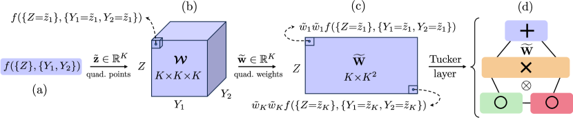
Given a candidate PIC, we will explore it in post order traversal, and iteratively associate a circuit layer (Definition 2) to each PIC unit, a process that we call materialization. We detail such procedure in Algorithm 3, which essentially applies Eq. 1 hierarchically over the PIC units. Each unit encodes a function over potentially continuous and discrete variables, hence representing a quasi-tensor, which we approximate by evaluating it over the quadrature points only, thus materializing a classical tensor (Fig. 3 (a,b)). We facilitate quadrature by assuming that all PIC LVs have bounded domain . This way, we can always use the same quadrature rule for each required (multivariate) approximation, and also simplify treatment and exposition.
We begin materializing every PIC input unit with function w.r.t. integration points , effectively creating an input layer as (Line 4, Algorithm 3). The parameters of such layer can be materialized as a matrix of shape , where is the number of parameters requires. For example, if is a univariate conditional Gaussian , we use a matrix for parameterizing the layer, where each row stores the mean and standard deviation at each integration point .
Next, we address the most important part of this quadrature process, i.e. the materialization of PIC integral units as sum layers. Specifically, let be an integral unit with -dimensional function , where and . We materialize w.r.t. integration points , effectively creating an -modes tensor , such that
| (2) |
After materializing tensor , we flatten it w.r.t. variables and , so as creating a matrix of size , an operation aka matricization. As last step, we plug-in the quadrature weights in , arriving to matrix of , whose -th row is
| (3) |
where is the vector of size resulting from the -times application of the Kronecker product over (Line 6, Algorithm 3). We illustrate this process in Fig. 3(a-c). Similarly, we also materialize every PIC sum unit with weights as a sum layer, but parameterized by
| (4) |
where is the identity matrix and the concatenation operator (Line 8, Algorithm 3). Note that such sum layer can be seen as a mixing layer [42, 39]. Finally, consider a PIC product unit with inputs and , each outputting functions with LVs and respectively. We associate to an Hadamard product layer if , or a Kronecker product layer if , reflecting the fact that we are marginalizing out two different LVs. We summarize our PIC materialization in Algorithm 3, where we iteratively associate a PIC unit to a circuit layer, eventually delivering a tensorized QPC. We will learn PICs via maximizing the likelihood of its QPC materialization.
QPCs as existing tensorized architectures.
Materializing PICs built via Algorithm 1 delivers tensorized PCs with alternating sum and product layers, aka sum-product layers [39]. An instance of such layers is the Tucker layer, used in architectures like RAT-SPNs [43] and EiNets [42]. Specifically, a binary Tucker layer [51] computes
| (Tucker-layer) |
where and are input layers of , each outputting a -dimensional vector. In contrast, the recent HCLT architectures [31] use the canonical polyadic (CP) layer [2], i.e.
| (CP-layer) |
where . We exactly recover Tucker (resp. CP) layers in our QPCs when these are materialized from PICs built via Tucker-merge (resp. CP-merge) in Algorithm 2, and hence the name of the merging procedure. Therefore, some QPCs can exactly match existent tensorized architectures, and this certainly happens when these are materialized from PICs built via Algorithm 1. This gives a new point of view on traditional tensorized architectures, and new possibilities for representation learning [54]. Figure 3 illustrates how the materialization of a 3-variate function leads to a Tucker layer. This 1-to-1 mapping between tensorized PC architectures and QPCs will allow for a fair comparison in our experiments.
Folding tensorized circuits for faster inference.
The layers of a tensorized circuit that (i) share the same functional form and that (ii) can be evaluated in parallel, can be stacked together as to create a folded layer [39, 42] which speeds up inference and learning on GPU by orders of magnitude. For instance, let be parallelizable Tucker layers each parameterized by a matrix of size . Such layers can be evaluated as a folded layer parameterized by a tensor of size , which computes the—otherwise sequential— tucker layers in parallel. We illustrate folding in Fig. 2(d), and later on in Fig. 4(c). Note that (i) the input layers sharing the same function form can always be folded and that (ii) although a tensorized circuit may have many types of sum-product layers, using one type only is common in practice, and promotes depth-wise folding.
3.3 Scaling PICs with neural functional sharing
Materializing QPCs can be memory intensive and time consuming, depending on: (i) the cost of evaluating the functions we need to materialize, (ii) the degree of parallelization of the required function evaluations, and (iii) the number of integration points . To solve these issues, we introduce neural functional sharing [47], i.e. we share multi-layer perceptrons as to parameterize multiple PIC units at once. This allows us to scale to larger models and datasets, as we make materialization faster and more memory-efficient than previous work [18].
PIC functional sharing.
functional sharing is to PICs as parameter-sharing is to PCs. This type of sharing can be applied over a group of input/integral units—grouped according to some criteria—whose functions have all the same number of input and output variables. Specifically, let be a group of input/integral units, each with function . The simplest form of functional sharing is to set all functions to be equal, i.e. . In this way, we reduce the number of function evaluations from to as long as we materialize each w.r.t. the same integration points , which is the case for Algorithm 3. We call this type of sharing F-sharing, as per full-sharing. More interestingly, leveraging functional composition, we may define , so as sharing an inner function for all unit functions. Similarly as before, as long as we materialize each w.r.t. the same quadrature points , we would only need function evaluations for instead of , as we can share them with all outer functions for further evaluation. We call this type of sharing C-sharing, as per composite-sharing. The original implementation of PICs [18] used neither F-sharing nor C-sharing.
Finally, we present and apply two different ways of grouping units. The first consists of grouping all input units, a technique which is only applicable when all input variables share the same domain. With this grouping, coupled with F-sharing, we would only need to materialize parameters, and use them to parameterize every QPC input layer. The second consists of grouping all integral units at the same depth of the PIC structure, which we couple with C-sharing and materialize as a folded sum-product layer. Despite grouping units that materialize into a folded layer is a natural and convenient choice, note that we can also group units that do not materialize as such. Once all units in a PIC have been grouped, materialization can be performed per-group.
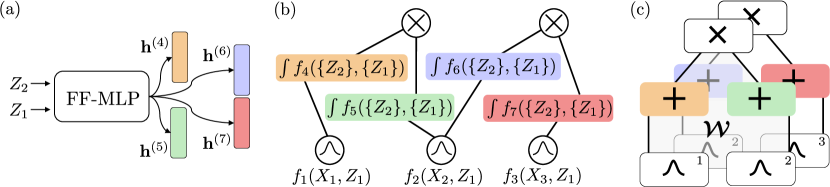
PIC functional sharing with (multi-headed) MLPs.
Similar to [18], we parameterize PIC input and integral units with light-weight multi-layer perceptrons (MLPs). However, instead of using a single MLP for each function, we will apply functional sharing as we strive to make the QPC materialization faster and memory efficient. Specifically, consider a group of integral units , each with function , over which we want to apply functional sharing. For every group , we would have an layered MLP of the form:
| (5) |
where is a Fourier-feature layer [48], and each is a standard linear layer followed by an element-wise non linearity , i.e. , with , and being the size of the MLP. Applying F-sharing over would simply consist of setting
| (neural F-sharing) |
where and are group-dependent parameters, therefore making all functions in the group equal. Instead, to implement C-sharing, we parameterize each as
| (neural C-sharing) |
where and are function-dependent parameters, effectively creating a multi-headed MLP. Fig. 4 illustrates our neural C-sharing and Section C.1 provides more details.
Fast & memory-efficient QPC materialization
Combing PIC functional sharing and per-group materialization allows scaling the training of PICs via numerical quadrature, as we drastically reduce the number and the cost of function evaluations required for the QPC materialization. We can now materialize very large QPCs, matching the scale of recent over-parameterized PCs yet requiring up to 99% less trainable parameters when using a large . This was not possible in the original formulation of PIC [18] as (i) the entire QPC was materialized in one-shot, not per-group, and (ii) no functional sharing was implemented, as each input/integral function had its own MLP.
4 Experiments
In our experiments, we first benchmark the effectiveness of functional sharing for scaling the training of PICs via numerical quadrature, comparing it with standard PCs and PICs w/o functional sharing [18]. Then, following prior work [10, 32, 33, 18], we compare QPCs and PCs as distribution estimators on several image datasets. We use an NVIDIA A100 40GB throughout our experiments.
Thanks to our pipeline, we can now use two recently introduced RGs tailored for image data which deliver architectures that scale better than those built out of classical RGs [45, 43, 31]: quad-trees (QTs), tree-shaped RGs, and quad-graphs (QGs), DAG-shaped RGs [39]. These are perfectly balanced RGs, and therefore applying Algorithm 1 over them would deliver balanced PIC structures amenable to depth-wise C-sharing of integral units. We report full details about QTs and QGs in Appendix B. We denote a tensorized architecture as [RG]-[sum-product layer]-[], e.g. QT-CP-16, which can be trained as a standard PC or materialized as QPC from a PIC. We treat pixels are categorical variables, and, as such, our architectures model probability mass functions.
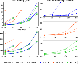
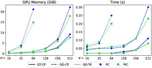
Scaling PICs.
For each model type, , we specify a pair where the first (resp. second) argument specifies the sharing technique, , for the input (resp. inner) layers/groups, where N stands for no sharing. In Fig. 5, we report the time and GPU memory required to perform an Adam [23] optimization step using PCs ( ), and PICs with ( ) and without ( ) functional C-sharing over the integral unit groups. We note that PICs using functional sharing ( ) proves very effective for scaling, requiring comparable resources as PCs ( ), while those who do not ( )—like prior work [18]—are orders of magnitude slower and quickly go Out-Of-Memory (OOM) for . Remarkably, some configuration of PICs ( ) require even less GPU memory than PCs, and this is because of the significant difference in the number of trainable parameters, since copies of these have to be stored by Adam during optimization. In fact, the number of parameters for PCs and PICs w/o functional sharing ( , ) is in the order of hundreds of millions (hitting 2B+), while PICs with functional sharing ( ) scale much more gracefully, hitting only 6M+ parameters. We emphasise that the number of trainable parameters of PICs is independent of the at which we materialize, but only dependent on the size of the MLPs we use to parameterize them, which can also be thought as the cost of evaluating PIC functions. We report more (tabular) details in Section D.1.
figurec
| QPC | PC | Sp-PC | HCLT | RAT | IDF | BitS | BBans | McB | |
|---|---|---|---|---|---|---|---|---|---|
| Mnist | 1.11 | 1.17 | 1.14 | 1.21 | 1.67 | 1.90 | 1.27 | 1.39 | 1.98 |
| f-mnist | 3.16 | 3.32 | 3.27 | 3.34 | 4.29 | 3.47 | 3.28 | 3.66 | 3.72 |
| emn-mn | 1.55 | 1.64 | 1.52 | 1.70 | 2.56 | 2.07 | 1.88 | 2.04 | 2.19 |
| emn-le | 1.54 | 1.62 | 1.58 | 1.75 | 2.73 | 1.95 | 1.84 | 2.26 | 3.12 |
| emn-ba | 1.59 | 1.66 | 1.60 | 1.78 | 2.78 | 2.15 | 1.96 | 2.23 | 2.88 |
| emn-by | 1.53 | 1.47 | 1.54 | 1.73 | 2.72 | 1.98 | 1.87 | 2.23 | 3.14 |
Distribution estimation.
Following prior work [10, 32, 33, 18], we extensively test QPCs and PCs as distribution estimators on standard image datasets. Our full results are in Section D.2, while we only report here the bits-per-dimension (bpd) of the best performing models, which always belong to a QG-CP architecture, reflecting the additional expressiveness of DAG-shaped RGs. Our full results also highlights how the the more expressive yet expensive Tucker layers we introduced for PICs deliver the best performance for small , but are hard to scale. All QPCs are materialized from PICs applying F-sharing over input units and C-sharing over groups of integral units, i.e. PIC (F, C). We begin with the Mnist-family, which includes 6 datasets of gray-scale 28x28 images: Mnist [29], FashionMnist [55], and EMNIST with its 4 splits [7]. Fig. 6 shows that QPCs generally perform best, improving over standard PCs (5/6), complex heuristic-based PC learning schemes as pruning-and-growing (5/6) [10], and some deep generative models (DGMs) (6/6).
Then, we move to larger RGB image datasets as CIFAR [28], ImageNet32, ImageNet64 [14], and CelebA [34]. To compare against prior work [32, 33], we have to preprocess the datasets using the YCoCg transform, a lossy color-coding that consistently improves performance for PCs when applied to RGB images.222The use of the lossy YCoCg transform is undocumented in [32, 33] but confirmed via personal communication with the authors. Note that columns in Table 1 using it () are not directly comparable to the rest. We also report results over datasets preprocessed with the lossless YCoCg-R transform [38], effectively doubling the number of datasets. We report details about these transforms in Section C.3. From Table 1, we see that QPCs prove again very competitive, consistently outperforming standard PCs commonly trained with Adam, and the best performing PC from the literature, HCLT, which is trained via EM schemes and patch-wise methods [32]. Furthermore, QPCs are close to PCs trained via latent variable distillation (LVD) [32, 33], a framework that requires extra supervision over their latent spaces by distilling information from existing deep generative models (DGMs). This technique requires pre-trained DGMs, several heuristics, and a final fine-tuning stage via EM or SGD, while PIC training method is instead end-to-end and self-contained.
| CIFAR | 5.09 | 5.50 | 4.48 | 4.85 | 4.61 | 4.37 | 3.87 |
|---|---|---|---|---|---|---|---|
| ImgNet32 | 5.08 | 5.25 | 4.46 | 4.63 | 4.82 | 4.38 | 4.06 |
| ImgNet64 | 5.05 | 5.22 | 4.42 | 4.59 | 4.67 | 4.12 | 3.80 |
| CelebA | 4.73 | 4.78 | 4.11 | 4.16 | - | - | - |
5 Discussion & Conclusion
With this work, we systematized the construction of PICs, extending them to DAG-like structures (Section 3.1), tensorizing (Section 3.2), and scaling their training with functional sharing (Section 3.3). In our experiments (Section 4), we showed how this pipeline is remarkably effective when the tractable approximations of PICs, QPCs, are used as distribution estimators. This in turn becomes a new and effective tool to learn PCs at scale. In fact, prior work has shown that naively training large PCs via EM or gradient-ascent is challenging, and that PC performance plateau as their size increases [10, 8, 32, 33]. Our contributions go beyond these limitations, while offering a simple, principled and fully-differentiable pipeline that delivers performance that rival more sophisticated alternatives [10, 32] (Section 4). We conjecture that this happens as training PCs via PICs drastically reduces the search space while allowing (i) smoother training dynamics and (ii) the materialization of arbitrarily large tractable models.
The development of tractable models is an important task in machine learning as they provide many inference routines, and can be used in many down-stream applications such as tabular data modelling [8], generative modelling [42], loss-less compression [30], genetics [11], knowledge-graphs [36], constrained text generation [58], and more. Our work has also certain parallels with tensor networks and (quasi-)tensor decompositions [51, 26, 22, 6, 49], as [39] recently showed how hierarchical tensor decompositions can be represented using the language of tensorized circuits. Furthermore, we note that the recent non-monotonic PCs [35] (i.e., PCs with negative sum parameters) can also be thought as the result of a quadrature process from PICs whose function can return negative values.
Our work does not come without limitations. Although we showed that training PICs with function sharing requires comparable resources as standard PCs, traditional continuous LV models as VAEs, flows and diffusion models are more scalable. Also, sampling from PICs is currently not possible, as we cannot perform differentiable sampling from our (multi-headed) MLPs. Future work may include the investigation of more efficient ways of training PICs, possibly using techniques as LVD or variational inference [24] to directly maximize PIC lower-bounds, requiring numerical quadrature only as fine-tuning step to distill a performant tractable model. We believe our work will foster new research in the field of generative modelling, and specifically in the realm of tractable models.
Acknowledgments
The Eindhoven University of Technology authors thank the support from the Eindhoven Artificial Intelligence Systems Institute and the Department of Mathematics and Computer Science of TU Eindhoven. Cassio de Campos thanks the support of EU European Defence Fund Project KOIOS (EDF-2021-DIGIT-R-FL-KOIOS). AV was supported by the "UNREAL: Unified Reasoning Layer for Trustworthy ML" project (EP/Y023838/1) selected by the ERC and funded by UKRI EPSRC. We thank Lorenzo Loconte for insightful discussions about (quasi-)tensor decompositions.
References
- [1] Cory Butz, Jhonatan S Oliveira, and Robert Peharz. Sum-product network decompilation. In International Conference on Probabilistic Graphical Models, pages 53–64. PMLR, 2020.
- [2] J. Douglas Carroll and Jih-Jie Chang. Analysis of individual differences in multidimensional scaling via an n-way generalization of “eckart-young” decomposition. Psychometrika, 35:283–319, 1970.
- [3] Myung Jin Choi, Vincent Y. F. Tan, Animashree Anandkumar, and Alan S Willsky. Learning latent tree graphical models. Journal of Machine Learning Research, 12(49):1771–1812, 2011.
- [4] YooJung Choi, Antonio Vergari, and Guy Van den Broeck. Probabilistic circuits: A unifying framework for tractable probabilistic models. Technical report, UCLA, 2020.
- [5] C. Chow and C. Liu. Approximating discrete probability distributions with dependence trees. IEEE Transactions on Information Theory, 14(3):462–467, 1968.
- [6] Andrzej Cichocki and Anh Huy Phan. Fast local algorithms for large scale nonnegative matrix and tensor factorizations. IEICE Trans. Fundam. Electron. Commun. Comput. Sci., 92-A(3):708–721, 2009.
- [7] Gregory Cohen, Saeed Afshar, Jonathan Tapson, and André van Schaik. EMNIST: Extending MNIST to handwritten letters. In IJCNN 2017, pages 2921–2926, 2017.
- [8] Alvaro Correia, Robert Peharz, and Cassio P de Campos. Joints in random forests. In Advances in Neural Information Processing Systems, volume 33, pages 11404–11415, 2020.
- [9] Alvaro H. C. Correia, Gennaro Gala, Erik Quaeghebeur, Cassio de Campos, and Robert Peharz. Continuous mixtures of tractable probabilistic models. Proceedings of the AAAI Conference on Artificial Intelligence, 37(6):7244–7252, 2023.
- [10] Meihua Dang, Anji Liu, and Guy Van den Broeck. Sparse probabilistic circuits via pruning and growing. In NeurIPS 2022, volume 35 of Advances in Neural Information Processing Systems, 2022.
- [11] Meihua Dang, Anji Liu, Xinzhu Wei, Sriram Sankararaman, and Guy Van den Broeck. Tractable and expressive generative models of genetic variation data. In Research in Computational Molecular Biology, pages 356–357, 2022.
- [12] Adnan Darwiche. Modeling and reasoning with Bayesian networks. Cambridge University Press, 2009.
- [13] Philip J. Davis and Philip Rabinowitz. Methods of numerical integration. Academic Press, 1984.
- [14] Jia Deng, Wei Dong, Richard Socher, Li-Jia Li, Kai Li, and Li Fei-Fei. Imagenet: A large-scale hierarchical image database. In 2009 IEEE conference on computer vision and pattern recognition, pages 248–255. Ieee, 2009.
- [15] Aaron W. Dennis and Dan Ventura. Learning the architecture of sum-product networks using clustering on variables. In Advances in Neural Information Processing Systems 25 (NeurIPS), pages 2033–2041. Curran Associates, Inc., 2012.
- [16] Nicola Di Mauro, Gennaro Gala, Marco Iannotta, and Teresa Maria Altomare Basile. Random probabilistic circuits. In 37th Conference on Uncertainty in Artificial Intelligence (UAI), volume 161, pages 1682–1691. PMLR, 2021.
- [17] Guido Fubini. Sugli integrali multipli. Rend. Acc. Naz. Lincei, 16:608–614, 1907.
- [18] Gennaro Gala, Cassio de Campos, Robert Peharz, Antonio Vergari, and Erik Quaeghebeur. Probabilistic integral circuits. In Proceedings of The 27th International Conference on Artificial Intelligence and Statistics, volume 238 of Proceedings of Machine Learning Research, pages 2143–2151. PMLR, 02–04 May 2024.
- [19] Robert Gens and Pedro M. Domingos. Learning the structure of sum-product networks. In International Conference on Machine Learning, 2013.
- [20] Ian Goodfellow, Jean Pouget-Abadie, Mehdi Mirza, Bing Xu, David Warde-Farley, Sherjil Ozair, Aaron Courville, and Yoshua Bengio. Generative adversarial nets. In NIPS 2014, volume 27 of Advances in Neural Information Processing Systems, 2014.
- [21] Emiel Hoogeboom, Jorn Peters, Rianne van den Berg, and Max Welling. Integer discrete flows and lossless compression. In NeurIPS 2019, volume 32 of Advances in Neural Information Processing Systems, 2019.
- [22] Yong-Deok Kim and Seungjin Choi. Nonnegative tucker decomposition. In CVPR. IEEE Computer Society, 2007.
- [23] Diederik P. Kingma and Jimmy Ba. Adam: A method for stochastic optimization. In ICLR 2015, 2015.
- [24] Diederik P. Kingma and Max Welling. Auto-encoding variational Bayes. In ICLR 2014, 2014.
- [25] Friso Kingma, Pieter Abbeel, and Jonathan Ho. Bit-swap: Recursive bits-back coding for lossless compression with hierarchical latent variables. In Proceedings of the 36th International Conference on Machine Learning, volume 97 of Proceedings of Machine Learning Research, pages 3408–3417, 2019.
- [26] Tamara G. Kolda. Multilinear operators for higher-order decompositions. Technical report, Sandia National Laboratories, 2006.
- [27] Daphne Koller and Nir Friedman. Probabilistic graphical models: principles and techniques. MIT press, 2009.
- [28] Alex Krizhevsky. Learning multiple layers of features from tiny images, 2009.
- [29] Yann LeCun, Corinna Cortes, and Christopher J. C. Burges. The MNIST database of handwritten digits, 2010.
- [30] Anji Liu, Stephan Mandt, and Guy Van den Broeck. Lossless compression with probabilistic circuits. In ICLR 2022, 2022.
- [31] Anji Liu and Guy Van den Broeck. Tractable regularization of probabilistic circuits. In NeurIPS 2021, volume 34 of Advances in Neural Information Processing Systems, pages 3558–3570, 2021.
- [32] Anji Liu, Honghua Zhang, and Guy Van den Broeck. Scaling up probabilistic circuits by latent variable distillation. In ICLR 2023, 2023.
- [33] Xuejie Liu, Anji Liu, Guy Van den Broeck, and Yitao Liang. Understanding the distillation process from deep generative models to tractable probabilistic circuits. In Proceedings of the 40th International Conference on Machine Learning, volume 202 of Proceedings of Machine Learning Research, pages 21825–21838, 2023.
- [34] Ziwei Liu, Ping Luo, Xiaogang Wang, and Xiaoou Tang. Deep learning face attributes in the wild. In Proceedings of International Conference on Computer Vision (ICCV), December 2015.
- [35] Lorenzo Loconte, M. Sladek Aleksanteri, Stefan Mengel, Martin Trapp, Arno Solin, Nicolas Gillis, and Antonio Vergari. Subtractive mixture models via squaring: Representation and learning. In The Twelfth International Conference on Learning Representations (ICLR), 2024.
- [36] Lorenzo Loconte, Nicola Di Mauro, Robert Peharz, and Antonio Vergari. How to turn your knowledge graph embeddings into generative models via probabilistic circuits. In Advances in Neural Information Processing Systems 37 (NeurIPS). Curran Associates, Inc., 2023.
- [37] Ilya Loshchilov and Frank Hutter. SGDR: Stochastic gradient descent with warm restarts. In ICLR 2017, 2017.
- [38] Henrique Malvar and Gary Sullivan. Ycocg-r: A color space with rgb reversibility and low dynamic range. ISO/IEC JTC1/SC29/WG11 and ITU-T SG16 Q, 6, 2003.
- [39] Antonio Mari, Gennaro Vessio, and Antonio Vergari. Unifying and understanding overparameterized circuit representations via low-rank tensor decompositions. In The 6th Workshop on Tractable Probabilistic Modeling, 2023.
- [40] Alejandro Molina, Antonio Vergari, Nicola Di Mauro, Sriraam Natarajan, Floriana Esposito, and Kristian Kersting. Mixed sum-product networks: A deep architecture for hybrid domains. In AAAI Conference on Artificial Intelligence, 2018.
- [41] Robert Peharz, Robert Gens, Franz Pernkopf, and Pedro Domingos. On the latent variable interpretation in sum-product networks. IEEE Transactions on Pattern Analysis and Machine Intelligence, 39(10):2030–2044, 2017.
- [42] Robert Peharz, Steven Lang, Antonio Vergari, Karl Stelzner, Alejandro Molina, Martin Trapp, Guy Van Den Broeck, Kristian Kersting, and Zoubin Ghahramani. Einsum networks: Fast and scalable learning of tractable probabilistic circuits. In 37th International Conference on Machine Learning (ICML), volume 119 of Proceedings of Machine Learning Research, pages 7563–7574. PMLR, 2020.
- [43] Robert Peharz, Antonio Vergari, Karl Stelzner, Alejandro Molina, Xiaoting Shao, Martin Trapp, Kristian Kersting, and Zoubin Ghahramani. Random sum-product networks: A simple and effective approach to probabilistic deep learning. In Proceedings of The 35th Uncertainty in Artificial Intelligence Conference, volume 115 of Proceedings of Machine Learning Research, pages 334–344, 2020.
- [44] Knot Pipatsrisawat and Adnan Darwiche. New compilation languages based on structured decomposability. In Proceedings of the 23rd National Conference on Artificial Intelligence (AAAI’08), volume 1, pages 517–522, 2008.
- [45] Hoifung Poon and Pedro Domingos. Sum-product networks: A new deep architecture. In IEEE International Conference on Computer Vision Workshops (ICCV Workshops), pages 689–690. IEEE, 2011.
- [46] Yangjun Ruan, Karen Ullrich, Daniel S. Severo, James Townsend, Ashish Khisti, Arnaud Doucet, Alireza Makhzani, and Chris Maddison. Improving lossless compression rates via monte carlo bits-back coding. In Proceedings of the 38th International Conference on Machine Learning, volume 139 of Proceedings of Machine Learning Research, pages 9136–9147, 2021.
- [47] Eran Segal, Dana Pe’er, Aviv Regev, Daphne Koller, Nir Friedman, and Tommi Jaakkola. Learning module networks. Journal of Machine Learning Research, 6(4), 2005.
- [48] Matthew Tancik, Pratul Srinivasan, Ben Mildenhall, Sara Fridovich-Keil, Nithin Raghavan, Utkarsh Singhal, Ravi Ramamoorthi, Jonathan Barron, and Ren Ng. Fourier features let networks learn high frequency functions in low dimensional domains. In NeurIPS 2020, volume 33 of Advances in Neural Information Processing Systems, pages 7537–7547, 2020.
- [49] Alex Townsend and Lloyd N Trefethen. Continuous analogues of matrix factorizations. Proceedings of the Royal Society A: Mathematical, Physical and Engineering Sciences, 471(2173):20140585, 2015.
- [50] James Townsend, Thomas Bird, and David Barber. Practical lossless compression with latent variables using bits back coding. In ICLR 2019, 2019.
- [51] L. R. Tucker. The extension of factor analysis to three-dimensional matrices. In Contributions to mathematical psychology., pages 110–127. Holt, Rinehart and Winston, 1964.
- [52] Antonio Vergari, YooJung Choi, Anji Liu, Stefano Teso, and Guy Van den Broeck. A compositional atlas of tractable circuit operations for probabilistic inference. In NeurIPS 2021, volume 36 of Advances in Neural Information Processing Systems, 2021.
- [53] Antonio Vergari, Nicola Di Mauro, and Guy Van den Broeck. Tractable probabilistic models: Representations, algorithms, learning, and applications, 2019. Tutorial at the 35th Conference on Uncertainty in Artificial Intelligence (UAI 2019).
- [54] Antonio Vergari, Robert Peharz, Nicola Di Mauro, Alejandro Molina, Kristian Kersting, and Floriana Esposito. Sum-product autoencoding: Encoding and decoding representations using sum-product networks. Proceedings of the AAAI Conference on Artificial Intelligence, 32(1), 2018.
- [55] Han Xiao, Kashif Rasul, and Roland Vollgraf. Fashion-MNIST: a novel image dataset for benchmarking machine learning algorithms. arXiv, 2017.
- [56] Ling Yang, Zhilong Zhang, Yang Song, Shenda Hong, Runsheng Xu, Yue Zhao, Wentao Zhang, Bin Cui, and Ming-Hsuan Yang. Diffusion models: A comprehensive survey of methods and applications. ACM Computing Surveys, 56(4):1–39, 2023.
- [57] Yang Yang, Gennaro Gala, and Robert Peharz. Bayesian structure scores for probabilistic circuits. In Proceedings of The 26th International Conference on Artificial Intelligence and Statistics, volume 206 of Proceedings of Machine Learning Research, pages 563–575, 2023.
- [58] Honghua Zhang, Meihua Dang, Nanyun Peng, and Guy Van den Broeck. Tractable control for autoregressive language generation. In 40th International Conference on Machine Learning (ICML), volume 202 of Proceedings of Machine Learning Research, pages 40932–40945. PMLR, 2023.
Appendix A Background on Circuits
Definition 3 (Circuit [4, 52]).
A circuit over variables is a parameterized computational graph encoding a function , and comprising three kinds of computational units: input, product, and sum. Each product or sum unit outputs a scalar and receives as inputs the output scalars of other units, denoted with the set . Each unit computes a function defined as: (i) if is an input unit, where is a function over variables , called its scope, (ii) if is a product unit, and (iii) if is a sum unit, with denoting the weighted sum parameters. The scope of a product or sum unit is the union of the scopes of its input units.
Definition 4 (Probabilistic Circuit).
A PC over variables is a circuit encoding a (possibly non-normalized) distribution, e.g., a function that is non-negative for all values of :
Definition 5 (Smoothness).
A circuit is smooth if, for each sum unit , its inputs depend on the same variables: .
Definition 6 (Decomposability).
A circuit is decomposable if the inputs of each product unit depend on disjoint sets of variables: .
Definition 7 (Structured-decomposability [44, 12]).
A circuit is structured-decomposable if (i) it is smooth and decomposable, and (2) any pair of product units having the same scope decompose their scope at their input units in the same way.
Although all tensorized architectures mentioned in this paper are smooth and decomposable, only PCs built from tree RGs are also structured-decomposable, and as such are potentially less expressive because they belong to a restricted class.
Appendix B Region Graphs
We detail in Algorithm B.1 the construction of the Quad-Tree (QT) and Quad-Graph (QG) region graphs [39]. Specifically, QTs (resp. QGs) are built setting the input flag isTree to True (resp. False). Intuitively, these RGs recursively split an image into patches, until reaching regions associated to exactly one pixel. The splitting is performed both horizontally and vertically, and subsequent patches can either be shared, thus yielding a RG that is not a tree (QGs), or not (QTs).
Input: Image height , image width , and whether to enforce the output RG to be a tree.
Output: A RG over variables
Input: A RG , a set of four coordinates , and a set of regions S
Behavior: It merges the regions indexed by in by forming a tree structure
Input: A RG , a set of four coordinates , and a set of regions S
Behavior: It merges the regions indexed by in by forming a DAG structure
Appendix C Implementation details
C.1 Multi-headed MLP details
A multi-headed MLP of size parameterizing a group of PIC units with functions of the form consists of:
-
1.
A Fourier-Features Layer (details below), i.e. a non-linear mapping ;
-
2.
Two linear layers followed by hyperbolic tangent as activation function, i.e. two consecutive non-linear mappings ;
-
3.
heads with Softplus non-linearity, i.e. different non-linear mapping .
Note that, if is a group of CP (resp. Tucker) integral units, then (resp. ), while the output dimension is always equal to 1. Instead, if the group is a group of input units, the input dimension is always equal to 1, while the output dimension is equal to the number of required parameters of the specific distribution, e.g. for Gaussians.
Such multi-headed MLP is implemented using grouped 1D convolutions, which allow a one-shot materialization of all the layer parameters associated to the group. We found that initializing all the heads to be equal improves convergence.
Fourier Feature Layer
Fourier Feature Layers (FFLs) are an important ingredient for the multi-headed MLPs. FFLs [48] enable MLPs to learn high-frequency functions in low-dimensional problem domains and are usually used as first layers of coordinate-based MLPs. FFLs transform input to
where is a hyper-parameter and vectors are non-learnable, randomly initialized parameters. FFLs have two main benefits: (i) They allow learning more expressive functions by avoiding over-smoothing behaviours, and (ii) they reduce the total number of trainable parameters when used instead of conventional linear layers as the initial layers in MLPs.
C.2 Training details
We train both PICs and PCs using the same training setup. Specifically, for each dataset, we perform a training cycle of optimization steps, after which we perform a validation step and stop training if the validation log-likelihood did not improve by nats after 5 training cycles. Using can avoid long trainings with negligible improvements. We report these common training hyper-parameters in Table C.1. We use Adam [23] and a batch size of 256 for all experiments.
PIC training
After some preliminary runs, we found that a learning rate of worked best, which we annealed towards using cosine annealing with warm restarts across 500 optimization steps [37]. We also apply weight decay with .
PC training
After some preliminary runs, we found that a constant learning rate of 0.01 worked best for all PC models, and for all datasets. We keep the PC parameters unnormalized, and, as such, we clamp them to a small positive value () after each Adam update to keep them non-negative, and subtract the log normalization constant to normalize the log-likelihoods.
| dataset | max num epochs | ||
|---|---|---|---|
| Mnist-family excl. emnist-by | 200 | 250 | 0 |
| emnist-by | 100 | 1000 | 0 |
| CIFAR | 200 | 250 | 0 |
| ImageNet32 | 50 | 2000 | 10 |
| ImageNet64 | 50 | 2000 | 30 |
| CelebA | 200 | 750 | 10 |
C.3 YCoCg color-coding transforms
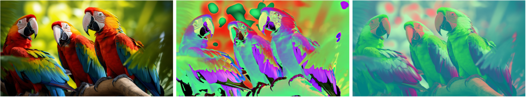
In Fig. C.1 and Fig. C.2 we provide pytorch code for the lossless and lossy versions of the YCoCg transform that we used in our experiments (Section 4). In Fig. C.3, we show how to apply them and that the lossy version is on average off less than a bit. Finally, in Fig. C.4 we show the significant visual difference of the two transforms when applied to an RGB image.
Appendix D Additional results
D.1 Scaling experiments
We report the time and GPU memory required to perform and Adamp optimization step for several model configurations in Table D.1, Fig. D.1 and Table D.2.
| RG-layer |
|
|
|
|
|
|||||||||||
| QT-CP | 0.02 | 0.02 | 0.02 | 0.02 | 0.07 | |||||||||||
| 0.02 | 0.02 | 0.02 | 0.02 | 0.07 | ||||||||||||
| 0.02 | 0.02 | 0.02 | 0.02 | 0.08 | ||||||||||||
| 0.02 | 0.02 | 0.03 | 0.03 | OOM | ||||||||||||
| 0.04 | 0.04 | 0.04 | 0.04 | OOM | ||||||||||||
| 0.08 | 0.08 | 0.11 | 0.12 | OOM | ||||||||||||
| QG-CP | 0.05 | 0.05 | 0.04 | 0.04 | 0.19 | |||||||||||
| 0.05 | 0.05 | 0.05 | 0.05 | 0.19 | ||||||||||||
| 0.06 | 0.06 | 0.05 | 0.05 | OOM | ||||||||||||
| 0.07 | 0.07 | 0.06 | 0.06 | OOM | ||||||||||||
| 0.11 | 0.11 | 0.11 | 0.11 | OOM | ||||||||||||
| 0.23 | 0.23 | 0.30 | 0.30 | OOM | ||||||||||||
| QG-TK | 0.07 | 0.07 | 0.06 | 0.06 | 0.15 | |||||||||||
| 0.09 | 0.09 | 0.08 | 0.08 | OOM | ||||||||||||
| 0.20 | 0.20 | 0.25 | 0.25 | OOM |
| RG-layer |
|
|
|
|
|
|||||||||||
| QT-CP | 0.11 | 0.14 | 0.15 | 1.01 | 2.69 | |||||||||||
| 0.21 | 0.28 | 0.21 | 1.05 | 6.97 | ||||||||||||
| 0.45 | 0.60 | 0.45 | 1.27 | 20.11 | ||||||||||||
| 1.02 | 1.31 | 1.06 | 1.93 | OOM | ||||||||||||
| 2.55 | 3.12 | 2.87 | 3.83 | OOM | ||||||||||||
| 7.62 | 8.39 | 9.13 | 10.09 | OOM | ||||||||||||
| QG-CP | 0.21 | 0.24 | 0.23 | 1.03 | 7.86 | |||||||||||
| 0.42 | 0.49 | 0.45 | 1.24 | 13.95 | ||||||||||||
| 0.93 | 1.07 | 0.97 | 1.79 | OOM | ||||||||||||
| 2.22 | 2.50 | 2.39 | 3.25 | OOM | ||||||||||||
| 5.93 | 6.50 | 6.85 | 7.66 | OOM | ||||||||||||
| 17.91 | 19.05 | 22.08 | 23.04 | OOM | ||||||||||||
| QG-TK | 0.70 | 0.72 | 0.81 | 1.55 | 18.60 | |||||||||||
| 2.99 | 3.04 | 3.78 | 4.37 | OOM | ||||||||||||
| 14.82 | 14.91 | 21.08 | 21.71 | OOM |
| QT-CP | QG-CP | QG-TK | |
|---|---|---|---|
| PIC | 1.1M | 2.2M | 1.8M |
| 270K | 800K | 6M | |
| 1M | 3M | 51M | |
| 4M | 13M | 408M | |
| 17M | 51.1M | - | |
| 69M | 204M | - | |
| 277M | 817M | - |
| RG-layer | PC (F, N) | PIC (F, C) | PIC (F, N) | |||||||
| QT-CP | 37 | 39 | 38 | 38 | 39 | 305 | 183 | 87 | 56 | |
| 50 | 51 | 50 | 51 | 51 | 354 | 147 | 116 | 69 | ||
| 75 | 76 | 75 | 75 | 76 | OOM | OOM | 242 | 114 | ||
| 127 | 126 | 126 | 125 | 126 | OOM | OOM | OOM | OOM | ||
| 249 | 258 | 254 | 253 | 251 | OOM | OOM | OOM | OOM | ||
| QG-CP | 73 | 68 | 68 | 68 | 69 | OOM | 512 | 218 | 119 | |
| 94 | 88 | 87 | 88 | 88 | OOM | 678 | 291 | 140 | ||
| 130 | 124 | 123 | 124 | 123 | OOM | OOM | OOM | 241 | ||
| 209 | 202 | 202 | 201 | 201 | OOM | OOM | OOM | OOM | ||
| 411 | 429 | 421 | 417 | 414 | OOM | OOM | OOM | OOM | ||
| QG-TK | 109 | 92 | 94 | 92 | 90 | OOM | OOM | 394 | 147 | |
| 188 | 180 | 176 | 175 | 173 | OOM | OOM | OOM | OOM | ||
| RG-layer | PC (F, N) | PIC (F, C) | PIC (F, N) | |||||||
|---|---|---|---|---|---|---|---|---|---|---|
| RG-layer | 1.04 | 0.89 | 0.87 | 0.86 | 0.86 | 13.87 | 5.03 | 2.14 | 1.32 | |
| 1.98 | 1.65 | 1.62 | 1.61 | 1.61 | 31.45 | 12.54 | 6.15 | 3.07 | ||
| 3.98 | 3.32 | 3.27 | 3.25 | 3.24 | OOM | OOM | 22.59 | 10.97 | ||
| 8.48 | 7.24 | 7.11 | 7.04 | 7.01 | OOM | OOM | OOM | OOM | ||
| 19.47 | 17.45 | 16.96 | 16.72 | 16.60 | OOM | OOM | OOM | OOM | ||
| QG-CP | 1.20 | 0.97 | 0.93 | 0.91 | 0.90 | OOM | 12.83 | 4.88 | 2.29 | |
| 2.44 | 1.87 | 1.82 | 1.79 | 1.78 | OOM | 27.72 | 12.93 | 6.16 | ||
| 5.30 | 4.10 | 3.99 | 3.95 | 3.92 | OOM | OOM | OOM | 22.13 | ||
| 12.51 | 10.24 | 9.94 | 9.80 | 9.72 | OOM | OOM | OOM | OOM | ||
| 32.92 | 29.29 | 28.22 | 27.69 | 27.42 | OOM | OOM | OOM | OOM | ||
| QG-TK | 2.62 | 2.54 | 2.45 | 2.41 | 2.39 | OOM | OOM | 22.97 | 11.10 | |
| 11.52 | 11.72 | 11.18 | 10.91 | 10.78 | OOM | OOM | OOM | OOM | ||
D.2 Additional distribution estimation results
In this section, we report tabular results for all our experiments.
Note that, every input layer of a standard PC is parameterized by a matrix , where is the number of categories, which is for grey-scale image datasets and for RGB images. We found that sharing a single input layer among all pixels results in (slightly) worse performance for grey-scale images (as detailed in Table D.3). In contrast, we found that such sharing considerably improves performance for RGB image datasets. Besides improving performance for RGB image datasets, such sharing considerably lower the number of trainable parameters from to only where is the number of pixels. For instance, parameterizing all input layers of a tensorized architecture with built for 64x64 images would require parameters, while only if we apply the sharing. Therefore, without applying such sharing, we cannot even scale to big tensorized architectures (e.g. QG-CP-512) on our GPUs.
All QPCs are materialized from PICs applying F-sharing over the group of input units, and C-sharing over the groups of integral units.
We extensively compare QPCs and PCs as density estimators on several image datasets and report test-set bits-per-dimension (bpd) in Table D.4, Table D.5 Table D.6 and Table D.7.
| QT-CP-512 | QG-CP-512 | QG-TK-64 | ||||
|---|---|---|---|---|---|---|
| w/o | w/ | w/o | w/ | w/o | w/ | |
| mnist | ||||||
| f-mnist | ||||||
| emn-mn | ||||||
| emn-le | ||||||
| emn-ba | ||||||
| emn-by | ||||||
| QT-CP | QG-CP | QG-TK | ||||
|---|---|---|---|---|---|---|
| QPC | PC | QPC | PC | QPC | PC | |
| OOM | ||||||
| OOM | ||||||
| OOM | ||||||
| OOM | ||||||
| OOM | ||||||
| OOM | ||||||
| QT-CP-512 | QG-CP-512 | QG-TK-64 | ||||
|---|---|---|---|---|---|---|
| QPC | PC | QPC | PC | QPC | PC | |
| mnist | ||||||
| f-mnist | ||||||
| emn-mn | ||||||
| emn-le | ||||||
| emn-ba | ||||||
| emn-by | ||||||
| QT-CP-512 | QG-CP-512 | QG-TK-64 | ||||
|---|---|---|---|---|---|---|
| QPC | PC | QPC | PC | QPC | PC | |
| QT-CP-256 | QG-CP-256 | QG-TK-32 | ||||
|---|---|---|---|---|---|---|
| QPC | PC | QPC | PC | QPC | PC | |