Continuum Attention for Neural Operators
Abstract
Transformers, and the attention mechanism in particular, have become ubiquitous in machine learning. Their success in modeling nonlocal, long-range correlations has led to their widespread adoption in natural language processing, computer vision, and time-series problems. Neural operators, which map spaces of functions into spaces of functions, are necessarily both nonlinear and nonlocal if they are universal; it is thus natural to ask whether the attention mechanism can be used in the design of neural operators. Motivated by this, we study transformers in the function space setting. We formulate attention as a map between infinite dimensional function spaces and prove that the attention mechanism as implemented in practice is a Monte Carlo or finite difference approximation of this operator. The function space formulation allows for the design of transformer neural operators, a class of architectures designed to learn mappings between function spaces, for which we prove a universal approximation result. The prohibitive cost of applying the attention operator to functions defined on multi-dimensional domains leads to the need for more efficient attention-based architectures. For this reason we also introduce a function space generalization of the patching strategy from computer vision, and introduce a class of associated neural operators. Numerical results, on an array of operator learning problems, demonstrate the promise of our approaches to function space formulations of attention and their use in neural operators.
Keywords: Operator Learning, Attention, Transformers, Discretization Invariance, Partial Differential Equations.
1 Introduction
Attention was introduced in the context of neural machine translation in Bahdanau et al. (2014) to effectively model correlations in sequential data. Many attention mechanisms used in conjunction with recurrent networks were subsequently developed, for example long short-term memory (Hochreiter and Schmidhuber, 1997) and gated recurrent units (Chung et al., 2014), which were then employed for a wide range of applications, see for example the review Chung et al. (2014). The seminal work Vaswani et al. (2017) introduced the now ubiquitous transformer architecture, which relies solely on the attention mechanism and not on the recurrence of the network in order to effectively model nonlocal, long-range correlations. In its full generality, the attention function described in Vaswani et al. (2017) defines an operation between sequences of lengths respectively, represented as tensors , where learnable weights parametrize
| (1) |
In this context, we recall that the function is defined component-wise via its action on the input as
| (2) |
for any . Therefore, in this form the attention function defines a mapping . 111We note that in most implementations, the input of the softmax function is rescaled by a factor of . In our context, continuum attention, a different scaling will be used. Alternatively, we can view the output of the attention function as a sequence .
Viewed more generally, attention defines a mapping from two sequences and into a third sequence ; all three sequences take values in for various values of . In this paper, we generalize this in two ways: (a) we replace index by index , where is a bounded open subset in ; (b) we retain a discrete index but allow the sequences to take values in Banach spaces of -valued functions defined over , where is a bounded open subset in . We find the first generalization (a) most useful in settings where , that is for time-series. However, when discretizing the index set with points, the quadratic scaling of the attention mechanism in can be prohibitive. This motivates generalization (b) where we retain the discrete index but allow sequences to be function valued, corresponding to patching of functions defined over , with
Our motivation for these generalizations is operator learning and, in particular, design of discretization invariant neural operator architectures. Such architectures disentangle model parameters from any particular discretization of the input functional data; learning is focused on the intrinsic continuum problem and not any particular discretization of it. This allows models to obtain consistent errors when trained with different resolution data, as well as enabling training, testing, and inference at different resolutions. We consider the general setting where is a bounded open set and and are separable Banach spaces of functions. To train neural operators we consider the following standard data scenario. The set of input-output observation pairs is such that is an i.i.d. sequence distributed according to the measure , which is supported on . We let and denote the marginals of on and respectively, so that and . In what follows, we consider to be an arbitrary map so that
| (3) |
noting that such maps will typically be both nonlocal (with respect to domain ) and nonlinear. We assume for simplicity that the data generation mechanism is compatible with (3) so that . Neural operators construct an approximation of picked from the parametric class
equivalently we may write for . The set is assumed to be a finite dimensional parameter space from which a is selected so that . We then define a cost functional and define by
| (4) |
In practice, we will only have access to the values of each and at a set of discretization points of the domain , which we denote as . We seek discretization invariant approaches to operator learning which allow for sharing of learned parameters between different discretizations.
The choice of an architecture defining the approximation family is sometimes known as surrogate modeling. We use continuum attention concepts to make this choice. The resulting transformer based neural operator methodology that we develop here can be used to learn solution operators to parametric PDEs, to solve PDE inverse problems, and may also be applied to solve a class of data assimilation problems. In the context of parametric PDEs we will explore how this algorithmic framework may be employed in operator learning for Darcy flow and 2d-Navier Stokes problems. As a particular case of operator learning, we will also explore a class of data assimilation problems that involve recovering unobserved trajectories of possibly chaotic dynamical systems. Namely, we illustrate examples involving the Lorenz-63 dynamical system and a controlled ODE.
1.1 Literature Review
The attention mechanism, as introduced in Vaswani et al. (2017) and defined in (1), has shown widespread success for a variety of tasks. In particular, given the suitability of attention and transformers for applications involving sequential data, there has been a large body of work extending the methodology from natural language processing, the setting in which it was originally introduced, to the more general context of time-series. Namely, as surveyed in Wen et al. (2023), transformers and variants thereof have been applied to time-series forecasting, classification and anomaly detection tasks. This generalization has involved modifications and innovations relating to the positional encoding and the design of the attention function itself. We refer the reader to Wen et al. (2023) for a detailed review of the large body of work and architectural variants of transformers that have been developed for time-series applications.
The quadratic scaling in the input of the attention mechanism has made transformers a computationally prohibitive architecture for applications involving long sequences. Nonetheless, through techniques such as patching, the attention mechanism and transformers have also enjoyed success in computer vision, where high-resolution image data presents an increased computational cost. In fact, in vision transformers (ViT), introduced in Dosovitskiy et al. (2021), the input image is subdivided into patches; attention is then applied across the shorter sequence of patches, thus decreasing the overall cost. Given the success of the methodology in computer vision, there has been growing interest in extending the transformer methodology to the operator learning context. This operator setting concerns learning mappings between infinite dimensional spaces of functions. In this case, the domains on which the functions are defined (spatial and temporal) may inherently be a continuum. Neural operators (Kovachki et al., 2023), generalizations of neural networks that learn operators mapping between infinite dimensional spaces, have been developed for this task. To this end, an integral kernel interpretation of the attention mechanism appearing for example in Tsai et al. (2019); Martins et al. (2020); Moreno et al. (2022); Wright and Gonzalez (2021); Cao (2021); Kovachki et al. (2023) inspired a range of attention-based architectures for operator learning. For example, the work of Cao (2021) leverages the integral kernel formulation to design novel attention mechanisms that do not require the softmax function. Inspired by the token mixing in attention functions, in Guibas et al. (2022) the authors propose an architecture for operator learning that involves token mixing in Fourier space. Various other approaches have been developed. In Li et al. (2023) the authors present a methodology relying on an encoder-decoder structure that employs self-attention and cross-attention and uses a recurrent multi-layer perceptron for unrolling instead of masked attention as in Vaswani et al. (2017). The work Hao et al. (2023) introduces an architecture for operator learning employing a normalized attention layer that handles multiple inputs. This design, along with a learned gating mechanism for input coordinates, allows the model to be applied to irregular meshes and multi-scale problems. In Ovadia et al. (2023) the authors propose to use an architecture composed of a ViT in the latent space of a U-Net (Ronneberger et al., 2015). The proposed model takes as input the input field evaluated on a grid with associated coordinate values and outputs an approximation of the solution to PDE inverse problems. While it is shown that the architecture achieves state-of-the-art accuracy, the parameters in the scheme are not invariant to the input function resolution. In the recent work Rahman et al. (2024), the authors propose a neural operator architecture that employs an attention mechanism that acts across channels of the function in the latent embedding, and do so in the context of pre-training a foundation model for PDE solution operators. We demonstrate how such an architecture can be derived from our formulation in Remark 16. As in our paper, various attention-related concepts are defined in a function-space setting, but our formulations are more general; this issue is discussed in detail at the relevant point in the paper.
The use of attention-based transformer models in the context of dynamical systems and data assimilation problems, where spatial and temporal domains of the systems are continuous, remains largely unexplored. For a comprehensive review on the application of machine learning to data assimilation we refer the reader to Cheng et al. (2023). In this context, the efficacy of transformers has been explored for forecasting in numerical weather prediction. In Chattopadhyay et al. (2022), a transformer module is integrated in the latent space of a U-Net (Ronneberger et al., 2015) architecture in order to leverage the permutation equivariance property of the transformer to improve physical consistency and forecast accuracy. The work in Bi et al. (2023) achieves state-of-the-art performance among end-to-end learning methods for numerical weather prediction by applying a ViT-like architecture and employing the shifted window methodology from Liu et al. (2021). The wide interest in blending ML and data assimilation along with the capability of transformer architectures provides an additional motivation for developing a mathematical framework for attention defined on infinite-dimensional spaces of functions.
Mathematical foundations for the methodology are only now starting to emerge, however most analysis has been preformed in the finite-dimensional setting. In the recent work Geshkovski et al. (2023), the authors study the attention dynamics by viewing tokens as particles in an interacting particle system. The formulation of the continuous-time limit of the dynamics, where the limit is taken in “layer time” allows to investigate the emergence of clusters among tokens. In Yun et al. (2020), the authors prove that transformers are universal approximators of continuous permutation equivariant sequence-to-sequence functions with compact support. More broadly, developing a firm theoretical framework for the subject is necessary to understand the empirical performance of the methodology and to inform the design of novel attention-based architectures.
1.2 Contributions and Outline
Motivated by the success of transformers for sequential data, we set out to formulate the attention mechanism and transformer architectures as mappings between infinite dimensional spaces of functions. In this work we introduce a continuum perspective on the transformer methodology. The resulting theoretical framework enables the design of attention-based neural operator architectures, which find a natural application to operator learning problems. The strength of the approach of devising implementable discrete architectures from the continuum perspective stems from the discretization invariance property that the schemes inherit. Indeed, the resulting neural operator architectures are designed as mappings between infinite dimensional functions spaces that are invariant to the particular discretization, or resolution, at which the input functions are defined. Notably, this allows for zero-shot generalization to different function discretizations. With these insights in view, our main contributions can be summarized as follows:
-
1.
Formulation of attention as a mapping between function spaces.
-
2.
Approximation theorem that quantifies the error between application of the attention operator to a continuous function and the result of applying its finite dimensional analogue to a discretization of the same function.
-
3.
A formulation of the transformer architecture as a neural operator, hence as a mapping between function spaces; the resulting scheme is resolution invariant and allows for zero-shot generalization to irregular, non-uniform meshes.
-
4.
A first universal approximation theorem for transformer neural operators.
-
5.
Formulation of patch-attention as a mapping between spaces of functions acting on patch indices. This continuum perspective leads to the design of efficient attention-based neural operator architectures.
-
6.
Numerical evidence of the competitiveness of transformer-based neural architectures.
After introducing, in Subsection 1.3, the notation that will be used throughout, Section 2 is focused on contributions 1 and 2, formulating attention as acting on functions defined on a continuous domain. In Section 3 we formulate the attention mechanism as acting on a sequence of “patches” of a function, addressing contribution 5. In Section 4 we make use of the operator frameworks developed in Sections 2 and 3 to formulate transformer neural operator architectures acting on function space. Thus we address 3, whilst the last two subsections concern the algorithmic aspect of extending to patching and address contribution 5. In Section 5 we state and prove a first universal approximation theorem for a transformer-based neural operator, hence addressing contribution 4. Finally, in Section 6 we explore applications of the transformer neural operator architectures to a variety of operator learning problems, contribution 6.
1.3 Notation
Throughout we denote the positive integers and non-negative integers respectively by and and the notation and for the reals and the non-negative reals. We let denote the set . For a set , we denote by the closure of the set, i.e. the union of the set itself and the set of all its limit points. We let denote the Euclidean inner-product and norm, noting that We may also use to denote the cardinality of a set, but the distinction will be clear from context. We write if we want to make explicit the dimension of the space on which the Euclidean inner product is computed. We will also denote by the norm on the vector space .
We denote by the infinite dimensional Banach space of continuous functions mapping the set to the -dimensional vector space . The space is endowed with the supremum norm. Similarly, we denote by the infinite dimensional space of square integrable functions mapping to . The space is endowed with the inner product, which induces the norm on the space. We will sometimes use the shorthand notation and to denote continuous functions and square integrable functions defined on the domain , respectively, when the image space is irrelevant. For integers we denote by the space of continuously differentiable functions up to order ; furthermore, for , we denote by the Sobolev space of functions possessing weak derivatives up to order of finite norm. Throughout, general vector spaces will be written using a calligraphic font . We denote by the infinite-dimensional space of linear operators mapping the vector space to the vector space . Throughout, we use different fonts to highlight the difference between operators acting on finite dimensional spaces, such as , and operators acting on infinite dimensional spaces, such as . We use to denote the Fourier transform, while will denote the inverse Fourier transform.
We use to denote expectation under the prevailing probability measure; if we wish to make clear that measure is the prevailing probability measure then we write .
2 Continuum Attention
In this section we formulate a continuum analogue of the attention mechanism described in Vaswani et al. (2017). We note that in the transformer architecture of Vaswani et al. (2017), a distinction is made between the self-attention and cross-attention functions. The former, a particular instance of (1) where , can be used to produce a representation of the input that captures intra-sequence correlations. On the other hand, cross-attention is used to output a representation of the input that models cross-correlations between both inputs and . Indeed, in Vaswani et al. (2017) cross-attention is employed in the decoder component of the transformer architecture so that the input to the decoder attends to the output of the encoder. For natural language applications in particular, the form of the cross-attention function has allowed for sequences of arbitrary length to be outputted from a transformer architecture while attending to sequences of different lengths, e.g. as outputs of length from a self-attention encoder block.
For pedagogical purposes we subdivide the presentation between the self-attention operator and the cross-attention operator, which are treated in Subsection 2.1 and Subsection 2.2 respectively. In Subsection 2.1.1 we define self-attention for discrete sequences indexed on finite bounded sets. Here, we outline the interpretation of self-attention as an expectation under a family of carefully defined discrete probability measures, each acting on the space of sequence indices. We show that under this formulation we recover the standard definition of self-attention from Vaswani et al. (2017). We proceed in Subsection 2.1.2 by formulating self-attention as an operator mapping between spaces of functions defined on bounded uncountable sets. This interpretation is natural, as functions may be thought of as “sequences” indexed over an uncountable domain. As in the discrete case, we formulate the self-attention operator as an expectation under a carefully defined probability measure acting on the domain of the input. We obtain an approximation result given by Theorem 6 that shows that for continuous functions the self-attention mechanism as implemented in practice may be viewed as a Monte Carlo approximation of the self-attention operator described. We mimic these constructions in Subsections 2.2.1 and 2.2.2 for the discrete and continuous formulations of cross-attention, respectively, and obtain an analogous approximation result given by Theorem 12. As in (1), throughout this section are learnable weights that parametrize the attention operators. When we consider self-attention we will have
2.1 Self-Attention
In the following discussion we define the self-attention operator in the discrete setting and in the continuum setting, in Subsections 2.1.1 and 2.1.2, respectively.
2.1.1 Sequences over
We begin by considering the finite, bounded set We let be a sequence and an index so that . We will now focus on formulating the attention mechanism in a manner which allows generalization to more general domains at the end of this subsection we connect our formulation with the more standard one used in the literature, which is specific to the current choice of domain We define the following discrete probability measure.
Definition 1
We define a probability measure on , parameterized by , via the probability mass function defined by
for any .
We may now define the self-attention operator as an expectation over this measure of the linear transformation applied to .
Definition 2
We define the self-attention operator as a mapping from a valued sequence over , , into a valued sequence over , , that takes the form
for any .
To connect these definitions with the standard formulation of transformers, note that sequence can be reformulated as the matrix Then
that is, the entry of is the right-hand side of the preceding identity, where denotes the ’th row of . It is then apparent that applying the softmax function along rows of delivers the vector of probabilities defined in Definition 1, indexed by note that is a parameter in this vector of probabilities, indicating the row of the matrix along which the softmax operation is applied. Finally the attention operation from Definition 2 can be rewritten to act between matrices as
so that .
Remark 3 (Sequences over )
Once the attention mechanism is formulated as in Definitions 1, 2, it is straightforward to extend to (generalized) sequences indexed over bounded subsets of note, for example, that pixellated images are naturally indexed over bounded subsets of Let possess cardinality Let be a sequence and an index. Then the definition of probability on , indexed by , and the resulting definition of self-attention operator , is exactly as in Definitions 1, 2. This shows the power of non-standard notation we have employed here.
2.1.2 Sequences over
We note that the preceding two formulations of the attention mechanism view it as a transformation defined as an expectation applied to the input sequence. The expectation is with respect to a probability measure supported on an index of the input sequence; furthermore the expectation itself depends on the input sequence to which it is applied, and is parameterized by the input sequence index, resulting in a new output sequence of the same length as the input sequence. The formulation using an expectation results from the softmax part of the definition of the attention mechanism; the query and key linear operations define the expectation, and the value linear operation lifts the output sequence to take values in a (possibly) different Euclidean space than the input sequence. These components may be readily extended to work with (generalized) sequences defined over open subsets of . (These would often be referred to as functions, but we call them generalized sequences to emphasize similarity with the discrete case.)
Let be an open set. Let be a sequence (function) and an index.
Definition 4
We define a probability measure on , parameterized by , via the probability density function defined by
for any .
Definition 5
We define the self-attention operator as a mapping from a valued sequence (function) over , , into a valued sequence (function) over , , as follows:
for any .
A connection between the discrete and continuum formulations of self-attention is captured in the following theorem.
Theorem 6
The self-attention operator may be viewed as a mapping and thus as a mapping . Furthermore, for any compact set ,
with the expectation taken over i.i.d. sequences .
Proof
The proof of this result is developed in Appendix A.1.
Remark 7
This result connects our continuum formulation of self-attention with the standard definition, using Monte Carlo approximation of the relevant integrals; a similar result could be proved using finite difference approximation on, for example, a uniform grid.
2.2 Cross-Attention
In the following discussion we define the cross-attention operator in the discrete setting and in the continuum setting, in Subsections 2.2.1 and 2.2.2, respectively.
2.2.1 Sequences over
We begin by letting and be finite sets of points with cardinalities and respectively. Let be a sequence (function), another sequence (function), and , indices so that and . We define the following discrete probability measure.
Definition 8
We define a probability measure on , parameterized by , via the probability mass function defined by
for any .
We may now define the cross-attention operator as an expectation over this measure of the linear transformation applied to .
Definition 9
We define the cross-attention operator as a mapping from a valued sequence (function) over , , and a valued sequence (function) over , , into a valued sequence (function) over , , as follows:
for any .
2.2.2 Sequences over
The framework described in Subsection 2.2.1 may be readily extended to work with generalized sequences (functions) defined over open subsets of . Indeed, let and be open sets. Let be a sequence (function), another sequence (function), and , indices. We define the following probability measure over before providing the definition of the cross-attention operator.
Definition 10
We define a probability measure on , parameterized by , via the probability density function defined by
for any .
Definition 11
We define the cross-attention operator as a mapping from a valued sequence (function) over , , and a valued sequence (function) over , , into a valued sequence (function) over , , as follows:
for any .
A connection between the discrete and continuum formulations of cross-attention is captured in the following theorem.
Theorem 12
The cross-attention operator may be viewed as a mapping , and so as a mapping . Furthermore, for any compact set
with the expectation taken over i.i.d. sequences .
Proof
The proof of this result is developed in Appendix A.2.
3 Continuum Patched Attention
Patches of a function are defined as the restriction of the function itself to elements of a partition of the domain. We may then define patch-attention as a mapping between spaces of functions defined on patch indices. Interest in applying the attention mechanism for computer vision led to the development of methodologies to overcome its prohibitive computational cost. Patching, as employed in vision transformers (ViT), involves subdividing the data space domain into “patches” and applying attention to a sequence of flattened patches. This step drastically reduces the complexity of the attention mechanism, which is quadratic in the input sequence length. An analogue of the patching strategy in vision transformers can be considered in the function space setting. Indeed, in image space, attention can be applied across subsets of pixels (patches); in function space, attention can be applied across the function defined on elements of a partition of the domain. Such a generalization to functions defined on the continuum allows for the development of architectures that are mesh-invariant. We describe the patched-attention methodology in the continuum framework developed thus far.
Throughout this section, we let be a bounded open set and let be a uniform partition of the space so that are congruent for all for some , where represents the number of patches. We consider a function defined on the full domain , denoted as . We define a mapping
| (5) |
that defines the patched version of the function , so that
| (6) |
for any . We proceed to establish the definitions of the patched self-attention operator in Subsection 3.1 and for completeness the patched cross-attention operator in Subsection 3.2.
3.1 Patched Self-Attention
We begin with the definition of the patched self-attention operator . Indeed, we let the operators be defined such that and let be an index.
Definition 13
Define a probability measure on , parameterized by , via the probability density function defined by
for any .222We note that as is linear, is shorthand notation for , and similarly for and .
Definition 14
The self-attention operator maps the function taking a patch index to a valued function over , , into a function taking a patch index to a valued function over , , as follows:
for any .
Remark 15 (Patched Attention in ViT)
An image may be viewed as a mapping , where , and where for grey-scale and for RGB-valued images. In the context of vision transformers (Dosovitskiy et al., 2021), the input to the attention mechanism is a sequence of “flattened” patches of the input image; we next outline the details to this procedure.
Letting be the total number of discretization points in and the number of patches, in the discrete setting each function patch may be represented as a matrix. The flattening procedure of each patch in ViT involves reshaping this matrix into a vector. The full image is thus represented as a sequence of vectors of dimension . Each patch vector is then linearly lifted to an embedding space of dimension . The embedded image, to which attention is applied, may hence be viewed as a matrix . Therefore, ViT may be cast in the setting of the discrete interpretation of the self-attention operator outlined in Subsection 2.1.1, where the domain on which attention is applied is . A key observation to the ensuing discussion is that the application of a linear transformation to a “flattened” patch in ViT breaks the mesh-invariance of the architecture; however, this operation may be viewed as a nonlocal transformation on each patch. We leverage this insight in Section 4 to design discretization invariant transformer neural operators that employ patching.
Remark 16 (Codomain Attention)
The work of Rahman et al. (2024) employs an attention mechanism that acts across the channels of the function in the latent space of a neural operator architecture. Indeed the “codomain” attention mechanism defined may be viewed as a particular variant of Definition 14, where , where is defined for and where are implemented as integral operators. In particular the indexing is by channels and not by patch. For problems in computer vision, similar ideas have been explored with discrete versions of the operators (Chen et al., 2017).
3.2 Patched Cross-Attention
For completeness, we outline the definition of the patched cross-attention operator. We consider to be a bounded open set and a uniform partition of so that for all for some and . We note that for the following construction we require , but it may hold in general that . As done for we define an operator
| (7) |
that defines the patched version of the function , so that
| (8) |
for any . Furthermore, we let the operators be defined such that and let be an index.
Definition 17
We define a probability measure on , parameterized by , via the probability density function defined by
for any .
Definition 18
The cross-attention operator maps the operator taking a patch index to a valued function over , , and the operator taking a patch index to a valued function over , , into an operator taking a patch index to a valued function over , , as follows:
for any .
4 Transformer Neural Operators
In this section we turn our attention to describing how to devise transformer-based neural operators using the continuum attention operator as defined in the function space setting in Section 2, and the continuum patched-attention operator acting on function space from Section 3. We make use of the operator frameworks developed in Sections 2 and 3 to formulate transformer neural operator architectures acting on function space. We start in Subsection 4.1, setting-up the framework. In Subsection 4.2 we formulate an analogue of the transformer from Vaswani et al. (2017) as an operator mapping an input function space to the solution function space . The resulting scheme is invariant to the discretization of the input function and allows for zero-shot generalization to irregular, non-uniform meshes. Motivated by the need to develop new efficient architectures to employ attention on longer sequences, or in our case higher resolution discretizations of functions, in Subsection 4.3 we describe a generalization of the ViT methodology to the function space setting, inspired by the work in Dosovitskiy et al. (2021). In particular we generalize the procedure of lifting flattened patches to the embedding dimension, as done in ViT, to the function space setting. This is achieved by lifting patches of functions to an embedding dimension using a nonlocal linear operator, namely, an integral operator. Unlike ViT, the resulting neural operator architecture is discretization invariant and allows for zero-shot generalization to different resolutions. In Subsection 4.4 we describe a different patching-based transformer neural operator acting on function space. The architecture is discretization invariant and is based on , learnable parameters in the attention mechanism, being defined as integral operators acting themselves on function space.
4.1 Set-Up
In the subsections that follow we describe transformer neural operators of the form , which serve as approximations to an operator . The neural operators we devise have the general form
| (9) |
for any and . In (9), the operators and are defined for some appropriate embedding function space . We will make explicit the definitions of the general operators , and the embedding function space in the context of each architecture. Throughout this section, we drop explicit dependencies on for brevity unless we wish to stress a parametric dependence; for example, we may abuse notation and write . The operator defines the neural operator analogue of the transformer encoder block from Vaswani et al. (2017). Its action on the input is summarized by the iteration
| (10a) | ||||
| (10b) | ||||
| (10c) | ||||
| (10d) | ||||
for layers, so that 333We note that we use to denote an arbitrary function in the space . This is not to be confused with used for cross-attention in Section 2. We also denote the output of the ’th encoder layer by , not to be confused with the notation used for the data pairs.. We note that for notational convenience, we have suppressed dependence of the operators on the layer ; indeed, each of the operators , and , will have different learnable parametrizations for each encoder layer . Before we delve into the specific neural operator architectures, we summarize the definitions of the elements of the transformer encoder described in (10), which are common to all the subsequent architectures. The multi-head self-attention operator is defined as the composition of a linear transformation applied pointwise to its input and a concatenation of the outputs of self-attention operators so that
| (11) |
for any . Here the notation indicates the ambiguity of the definition of self-attention. We note that we will make explicit which definition of self-attention operator from the previous sections we employ for each architecture; we will also make clear the definitions of the parameters defining each attention operator. The operators are pointwise linear operators. 444We note that for all experiments in Section 6 we set to be the identity operators. Next, the operator defines the layer normalization and the operator defines a feed-forward neural network layer. Both operators are applied pointwise to the input; further details are provided in the context of each architecture.
A key aspect of the ensuing discussion will be the distinction between local and nonlocal linear operators. We note that for an arbitrary function space where , the space of linear operators includes both local and nonlocal linear operators. In the following, we will consider pointwise linear operators in that admit a finite-dimensional representation . On the other hand, we will also consider linear integral operators in , a class of nonlocal operators. Namely, we consider operators that are integral operators learned from data of the form .
Definition 19 (Integral Operator )
The integral operator is defined as the mapping given by
| (12) |
where is a neural network parametrized by .
Assuming then (12) may be viewed as a convolution operator, which makes it possible to use the Fast Fourier Transform (FFT) to compute (12) and to parametrize in Fourier space. Following Li et al. (2021), this insight leads to the following formulation of the operator given in Definition 19.
Definition 20 (Fourier Integral Operator )
We define the Fourier integral operator as
| (13) |
To link to the definition (12) with translation-invariant kernel we take to be the Fourier transform of the periodic function parametrized by .
For uniform discretizations of the space , the Fourier transform can be replaced with the Fast Fourier Transform (FFT). Indeed, for the Fourier transform we have and . On the other hand, for the FFT we have and . In practice, it is possible to select a finite-dimensional parametrization by choosing a finite set of wave numbers
We can therefore parametrize by a complex -tensor.
These integral operator definitions will be used to define architectures for the Vision Transformer Neural Operator in Subsection 4.3 and the Fourier Attention Neural Operator in Subsection 4.4, but are not needed to define the basic Transformer Neural Operator in Subsection 4.2. In the context of each architecture, we make explicit the parametrizations of the integral operators employed.
4.2 Transformer Neural Operator
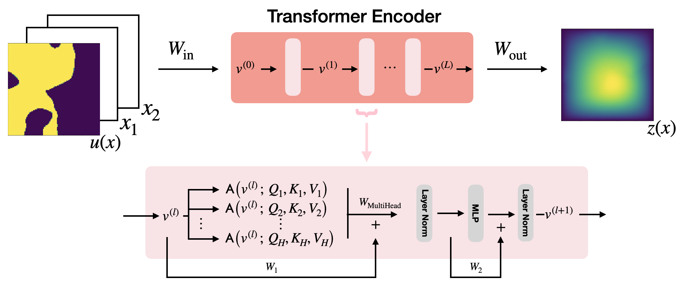
The transformer neural operator architecture follows the general structure of Equations 9 and 10; here, we make explicit the choices for that instantiate it. In Figure 1 we provide a schematic representation of the full transformer neural operator architecture. We consider model inputs , model embedding space , and model output space , with . The function is first concatenated with the identity defined on the domain , so that the resulting function is defined by its action on as
| (14) |
In practice, this step defines a positional encoding that is appended to the input function. A linear transformation is then applied pointwise to lift the function into the embedding space . The input operator is hence defined as
| (15) |
for defined as in (14), where , , and . Observe that acts as a local, pointwise linear operator on .
Next, we define the details of in Equation 10 by specifying a definition of , , , and for the transformer neural operator setting. The operator is the multi-head attention operator from (11) based on the continuum self-attention from Definition 5. Letting denote the number of attention heads, the multi-head attention operator is parametrized by the learnable linear transformations , for , where for implementation purposes is chosen as . 555We note that and should be chosen so that is a multiple of . The multi-head attention operator is thus defined by the application of a linear transformation to the concatenation of the outputs of self-attention operators. The operators are pointwise linear operators and hence admit finite-dimensional representations , so that they define a map
for each , and similarly for . The operator is defined such that
| (16) |
for , any , and any , where the notation is used to denote the ’th entry of the vector. In equation (16), is a fixed parameter, are learnable parameters and are defined as
| (17) | ||||
for any The operator is defined such that
| (18) |
for any and , where and are learnable parameters and where is a nonlinear activation function.
Finally, we define the output operator as a local linear operator applied pointwise, so that
| (19) |
for , and .
The composition of the operators completes the definition of the transformer neural operator. In Appendix B.1 we outline how this neural operator architecture is implemented in the finite-dimensional setting, where the input function is defined on a finite set of discretization points .
4.3 Vision Transformer Neural Operator
We introduce an analogue of the vision transformer architecture as a neural operator using the patching in the continuum framework developed in Section 3. We note that in the context of the ViT from Dosovitskiy et al. (2021), performing patch “flattening” before a local lifting to the embedding dimension introduces a nonlocal transformation on the patches, as described in Remark 15. This procedure as implemented in Dosovitskiy et al. (2021) violates the desirable (for neural operators) discretization invariance property. Hence, for a neural operator analogue, we substitute the lifting to embedding dimension with a nonlocal integral operator. The ViT neural operator (ViT NO) introduced is thus discretization invariant. We describe this methodology within the framework provided by making explicit choices for that instantiate Equations 9 and 10 appropriately. In Figure 2 we provide a schematic for the architecture, with a graphical representation of the encoder layer in Figure 3.
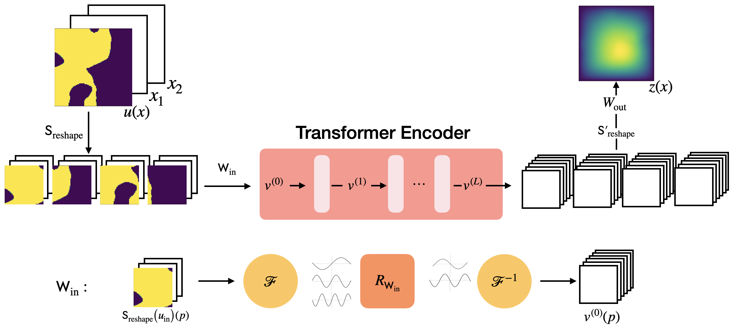
Let be a bounded open set. Consider and let be a uniform partition of the space so that for all for some , where represents the number of patches. We consider model inputs , model embedding space which is a space of functions acting on patch indices, and model output space , with domain .
We begin by defining the input function . The function is first concatenated with the identity defined on the domain , so that the resulting function is defined as in (14); recall that this defines a positional encoding. An operator is applied to the function that acts on the input so that the resulting function is of the form
| (20) |
We apply a nonlocal linear operator that acts on any so that for any
| (21) |
The above nonlocal linear operator is chosen as an integral operator as in Definition 20 and the subsequent discussion. The composition of the operators defined in Equations 14, 20 and 21 defines our choice of . Namely, we define via
| (22) |
Next, we define the details of in Equation 10 by specifying a definition of , , , and in this patched setting. In each layer the operator is the multi-head attention operator from (11) based on the self-attention from Definition 14. Letting denote the number of attention heads, the multi-head attention operator is parametrized by learnable local (pointwise) linear operators for . In this setting, these are chosen to be linear operators applied pointwise, they can be represented by finite dimensional linear transformations , for . 666We note that in the context of the Fourier attention neural operator, presented in the next Subsection 4.4, we generalize this definition to for being nonlocal linear integral operators. For implementation purposes is chosen as . 777We note that and should be chosen so that is a multiple of . The multi-head attention operator is thus defined by the application of a local linear transformation to the concatenation of the outputs of self-attention operators. The operators are pointwise linear operators and hence admit finite-dimensional representations , so that they define a map
| (23) |
for each and , and similarly for . The operator is defined such that
| (24) |
for , any and any , where we use the notation to denote the ’th entry of the vector. In equation (24), is a fixed parameter, are learnable parameters and are defined as in (17). The operator is defined by
| (25) |
for any and any , where and are learnable parameters and is a nonlinear activation function.
Finally, we define the action of . This is given by first applying a reshaping operator to the output of the encoder, where this map is defined as
| (26) |
We note that the operator may be viewed as an inverse of . A pointwise linear transformation defined by
| (27) |
for any , is then applied. This procedure completes the definition of the operator , which is given by
| (28) |
for any and .
Remark 21
We have found that adding a convolution in residual form helps to ameliorate the discontinuities arising when the patching architecture is used; these are visible in error plots and can also interfere with self-composition of maps learned as solution operators of time-dependent PDEs. To this end define the linear integral operator , of the form described in Definition 20 and the subsequent discussion, and add a last layer to the output of the architecture as defined thus far:
| (29) |
for .
The composition of the operators completes the definition of the ViT neural operator. In Appendix B.2 we outline how this neural operator architecture is implemented in the finite-dimensional setting, where the input function is defined on a finite set of discretization points .
4.4 Fourier Attention Neural Operator
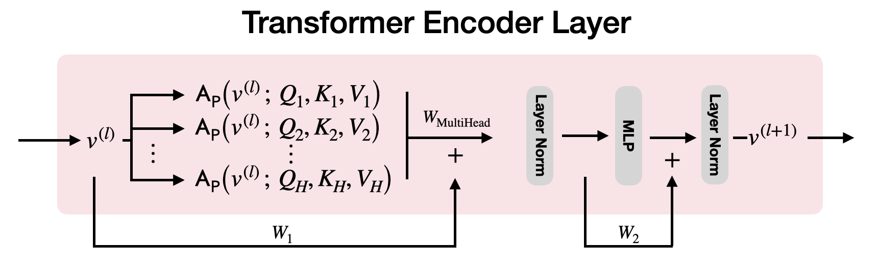
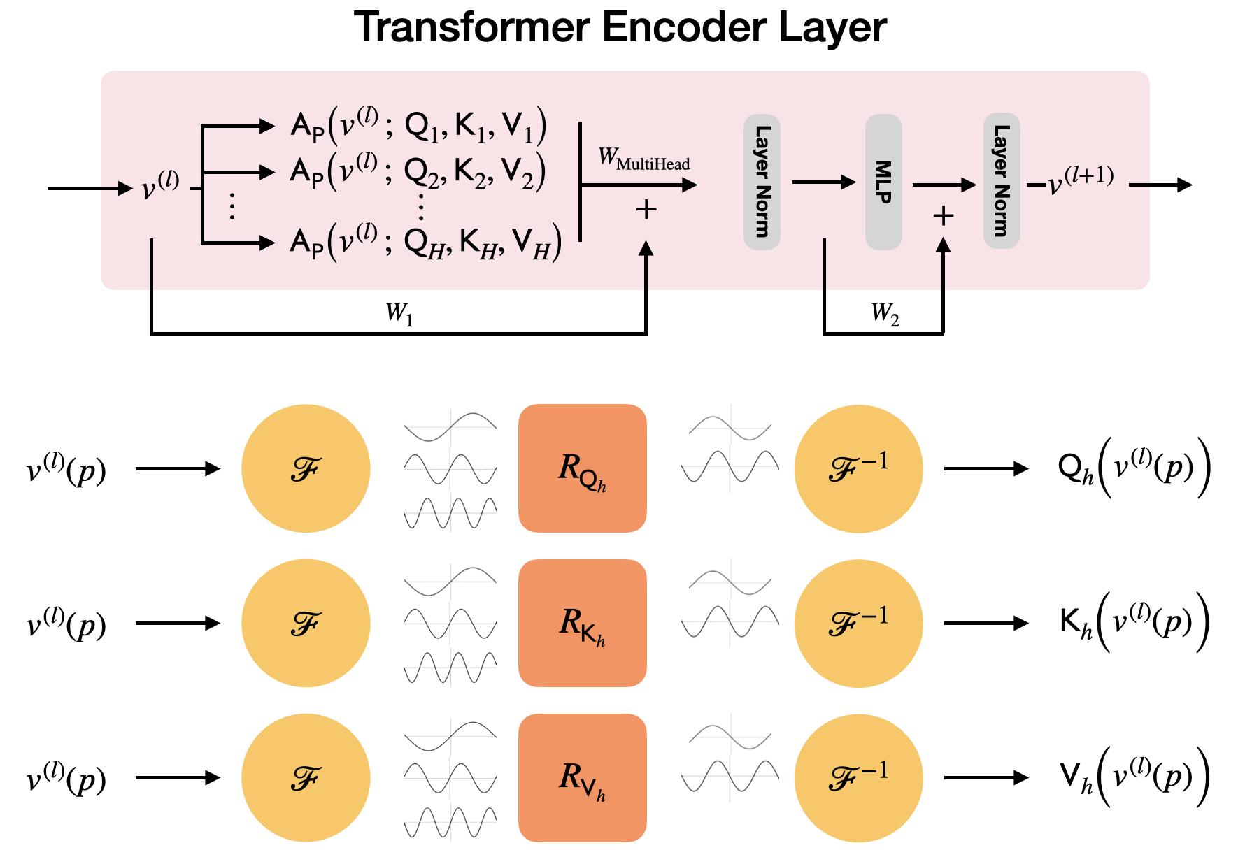
In this subsection, we introduce a different transformer neural operator based on patching, the Fourier attention neural operator (FANO). In this setting, to gain additional expressivity, we replace the local linear operators in the attention mechanism with nonlocal integral operators. In Figure 4 we provide a schematic for the Fourier attention neural operator architecture, with a graphical representation of the encoder layer in Figure 5. We outline the details of the architecture in the following discussion.
We again let be a bounded open set. Consider and let be a uniform partition of the space so that for all for some , where represents the number of patches. We consider model inputs , model embedding space which is a space of functions acting on patch indices , and model output space , with domain .
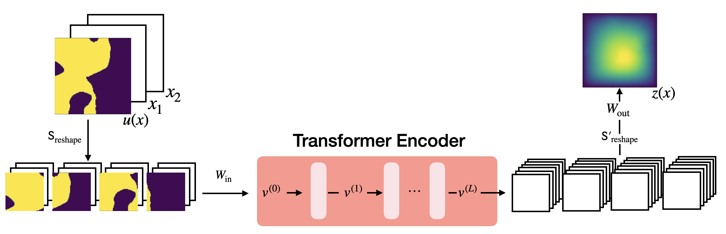
We define similarly to (22) in the previous section, via a composition of Equations 14, 20 and 21; however here the linear lifting operator is chosen to be a pointwise linear transformation . Namely, we define via
| (30) |
for any and any , where is defined as in (14), as in and the nonlocal operation (21) is replaced by a local pointwise one.
Next, we define the particulars of in Equation 10. The key distinction between the Fourier attention neural operator that we define here and the ViT neural operator from the previous subsection 4.3 lies in the nonlocality of operations performed within . Here, in each layer the operator is the multi-head attention operator from (11) based on the self-attention operator from Definition 14. Letting denote the number of attention heads, the multi-head attention operator is parametrized by learnable nonlocal linear integral operators and , for , where for implementation purposes is chosen as . The specific formulation of these linear integral operators may be found in Definition 20 and the subsequent discussion. The multi-head attention operator is thus defined by the application of a pointwise linear transformation to a concatenation of the outputs of self-attention operators. The operators are defined as in (23). The layer normalization operator is defined as in (24) so that it is applied to every point in every patch. Furthermore, the operator is defined as in (25).
We define identically to Equation 28. We refer to Remark 21 for an additional operation that can be applied to ameliorate the effect of patch discontinuities. Finally, the composition of the operators completes the definition of the Fourier attention neural operator. In Appendix B.3 we outline how this neural operator architecture is implemented in the finite-dimensional setting, where the input function is defined on a finite set of discretization points .
5 Universal Approximation by Transformer Neural Operators
Universal approximation is a minimal requirement for neural operators. When the operator to be approximated maps between spaces of functions defined over Euclidean domains, universal approximation necessarily requires both nonlocality and nonlinearity. In the recent paper Lanthaler et al. (2023), a minimal architecture possessing these two properties is exhibited. In this section, rather than trying to prove universal approximation for the various discretization-invariant neural operators introduced in the paper, we construct a simple canonical setting that exhibits the universality of the attention mechanism on function space, allowing direct exploitation of the ideas in Lanthaler et al. (2023). We build on the notation used in Subsection 4.1. In particular denotes the self-attention operator from Definition 5 and an activation function. Throughout this section, we consider activation functions which are non-polynomial and Lipschitz continuous.
To be specific, we consider neural operators of the form
| (31) |
where and are defined by neural networks of the form
| (32) | ||||
| (33) |
where and , where are learned linear transformations of appropriate dimensions and are learned vectors. We define the operator as a variant of the layer defined by the iteration step in Equation 10, given by the two-step map acting on its inputs as
| (34a) | ||||
| (34b) | ||||
for any . Note that the neural operator thus defined does not include layer normalizations; it is thus a variant of the transformer neural operator from Subsection 4.2. We may now apply the result of Lanthaler et al. (2023) to show two universal approximation theorems for the resulting transformer neural operator.
Theorem 22
Let be a bounded domain with Lipschitz boundary, and fix integers . If is a continuous operator and a compact set, then for any , there exists a transformer neural operator so that
| (35) |
Proof We begin by noting that for and , the self-attention mapping reduces to
| (36) |
For weights , and , the transformer encoder neural operator layer (34) reduces to the mapping
| (37) |
The existence of so that satisfies (35) then follows from Lanthaler et al. (2023, Theorem 2.1), which also involves the application of the universality result for two-layer neural networks of Pinkus (1999, Theorem 4.1).
The analysis in Lanthaler et al. (2023) allows the derivation of an analogous universal approximation theorem for functions belonging to Sobolev spaces. This generalization is the content of the next theorem. The proof follows easily by applying the same argument as in the proof of Theorem 22 and the result of Lanthaler et al. (2023, Theorem 2.2).
Theorem 23
Let be a bounded domain with Lipschitz boundary and fix integers , . If is a continuous operator and a compact set of bounded functions so that , then for any , there exists a transformer neural operator so that
| (38) |
6 Numerical Experiments
In this section we illustrate, through numerical experiments, the capability of the transformer neural operator architectures described in Section 4. Throughout, we consider the supervised learning problem described by the data model in (3) and take the viewpoint of surrogate modeling to construct approximations of the operators . In Subsection 6.1 we consider problems given by dynamical systems and ordinary differential equations, namely operators acting on functions defined on a one-dimensional time domain. In this context, we explore the use of the transformer neural operator for operator learning problems given by the Lorenz ‘63 dynamical system and a controlled ODE. On the other hand, in Subsection 6.2 we consider problems given by partial differential equations equations, namely operators acting on functions defined on a two-dimensional spatial domain. In this context we explore the use of the transformer neural operator and of the more efficient ViT neural operator and Fourier attention neural operator architectures for operator learning problems given by the Darcy flow and Navier-Stokes equations.
Remark 24 (Relative Loss)
For each neural operator architecture we optimize for the parameters according to the relative loss, i.e.
| (39) |
for data points .
6.1 1D Time Domain
In this subsection we consider problems where attention is applied to functions in the one-dimensional time domain. The first setting we consider is that of the Lorenz ‘63 dynamical system (Lorenz, 1963), a simplified model for atmospheric convection. The dynamics are given by
| (Lorenz ‘63) | ||||
We consider learning the operator given by
| (40) |
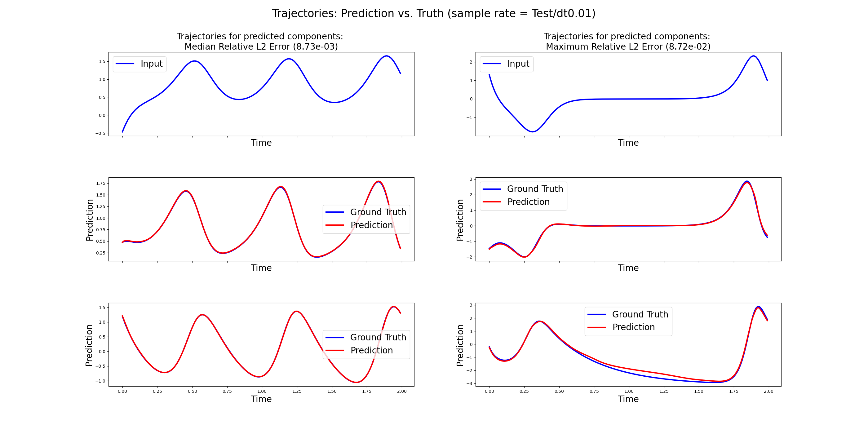
In this case, is known to exist and given by the solution operator for the system of linear ODEs arising from the second and third components of (Lorenz ‘63), given known first component. We note that including the initial condition of the unobserved trajectories in the model introduces a discrepancy in dimension within the input function to the model. Namely, denoting by the input to the model, while for . We overcome this issue by learning separate embedding linear transformations and , for the initial condition and the rest of the trajectory, respectively.In Figure 6 we display the results obtained by applying a transformer neural operator model on a test data set of samples with the same discretization ( and ) as the training set of samples on the operator learning problem described by (40). The operator is successfully learned, and displays median relative error of less than , with worst case rising to just below
We also experiment with a setting for which is not well-defined: we study the recovery of unobserved trajectory from the observed trajectory so that and
This operator would only be well-defined if were included as inputs. We nonetheless expect accurate recovery of the hidden trajectory by the property of synchronization (Pecora and Carroll, 1990; Hayden et al., 2011).
We investigate an additional operator learning problem given by the setting of the controlled ODE
| (CDE) | ||||||
In this case we aim to approximate the operator defined by
For this problem we make the choice .
The experimental settings we consider for the continuous time operator learning problem may be viewed from the lens of data assimilation as smoothing problems (Sanz-Alonso et al., 2023). Indeed, the mappings to be learned represent the recovery of an unobserved trajectory conditioned on the observation of a whole trajectory .
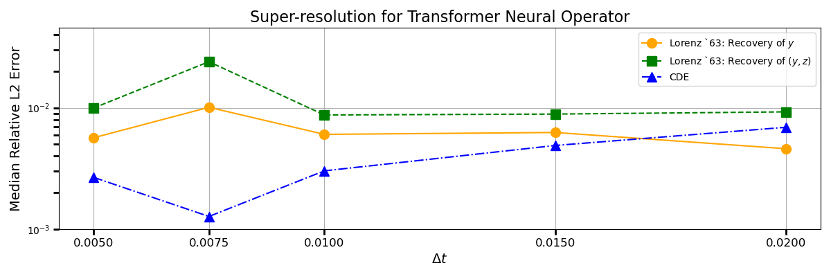
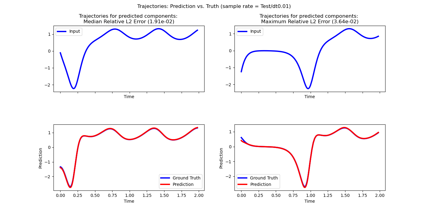
In Figure 7 we demonstrate the mesh-invariance property of the transformer neural operator in the context of the operator learning problems arising from equations (Lorenz ‘63) and (CDE). A key motivation for considering the continuum formulation of attention and the related transformer neural operator is the property of zero-shot generalization to different non-uniform meshes. To demonstrate this, in Figure 8 we consider the operator learning problem of mapping the observed trajectory of (Lorenz ‘63) to the unobserved trajectory. We display the median relative error and worst error samples from a test set consisting of trajectories , where the test time index set is defined as
| (41) |
for , where the model deployed is trained on trajectories indexed at a set defined by
| (42) |
In other words, the second half of the testing domain is up-sampled by a factor of 2 compared to the training discretization. As seen qualitatively in Figure 8 testing on the non-uniform discretization based on a model trained on the uniform grid is successful. The use of different grids in test and train does leads to a larger error than the one incurred when they match (seen in Figure 7), but the errors remain small. It is our continuum formulation of attention from Section B.1 that enables this direct generalization; it would not be possible with standard methods.
6.2 2D Spatial Domain
In this subsection we study two different 2D operator learning problems – flow in a porous medium, governed by the Darcy model, and incompressible viscous fluid mechanics governed by the Navier-Stokes equation, in particular, a Kolmogorov flow. We apply the three architectures developed in Sections 2 and 3, concentrating on the patched architectures. In the first Subsection 6.2.1 we report the results obtained by applying the neural operators described to an array of operator learning problems, where the domain of the functions is two-dimensional i.e. . In Subsection 6.2.2 we describe the settings of the two Darcy flow operator learning problems considered, along with the parametrization and training details for the various architectures. Similarly in Subsection 6.2.3, we describe the Kolmogorov flow operator learning problem and relevant implementation details. Subsections 6.2.2 and 6.2.3 also contain further numerical results illustrating the behaviour of the proposed transformer neural operators, and discretization invariance in particular.
6.2.1 Results
The results presented concern the two variants of Darcy flow, with lognormal and piecewise constant inputs, and the Kolmogorov flow. The operator learning architectures we deploy include the three transformer-based methods introduced in this paper, and the implementations of the Fourier neural operator from the “NeuralOperator” library (Li et al., 2021; Kovachki et al., 2023).
Our first results compares the transformer neural operator from Subsection 4.2 with FNO on the lognormal Darcy Flow problem in a low resolution setting. Table 1 provides a brief summary of the test relative errors obtained. It is notable that the transformer architecture obtains performance similar to FNO, despite not using patching, and with an order of magnitude fewer parameters. However since higher resolution renders the architecture from Subsection 4.2 impractical in dimensions the remainder of our experiments use the patched ViT and Fourier attention neural operators from Subsections 4.3 and 4.4 respectively.
| Architecture | Number of Parameters | Darcy Flow |
|---|---|---|
| Lognormal Input | ||
| Transformer NO | ||
| FNO |
We now consider training two patched architectures on the Darcy Flow problem with piecewise constant inputs and the Kolmogorov Flow problem; in both cases we use a resolution setting. We compare cost versus accuracy for the different neural operators implemented, defining cost in terms of both number of parameters and number of FLOPS. In Table 2 we present the FLOPS for each method; details of the derivation are provided in Appendix C. We note that the parameter scaling for the transformer neural operator is given by , while the scaling for the FNO and the Fourier attention neural operator is , where is the total number of Fourier modes used. The parameter scaling for the ViT neural operator is given by . Further details are provided in Appendix C.
| Architecture | Scaling |
|---|---|
| FNO | |
| Transformer NO | |
| ViT NO | |
| FANO |
Figures 9 and 10 display the cost-accuracy trade-off. Table 3 provides the test relative errors values, depicted in the cost-accuracy analysis figures, obtained with the models with the highest parameter count. Figure 9 demonstrates the parameter-efficiency of the ViT neural operator in comparison with both the FNO and Fourier attention neural operator. Once cost is defined in terms of FLOPS it is apparent that both patched transformer architectures outperform the FNO; furthermore the FNO exhibits accuracy-saturation, caused by the finite data set, whereas the patched architectures are less affected, in the ranges we test here. This suggests that the patched transformer architectures use the information content in the data more efficiently.
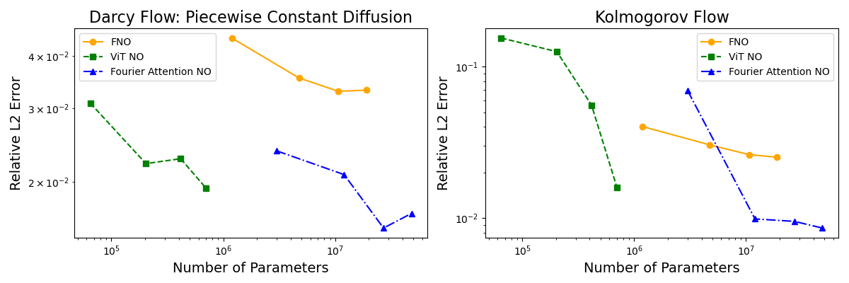
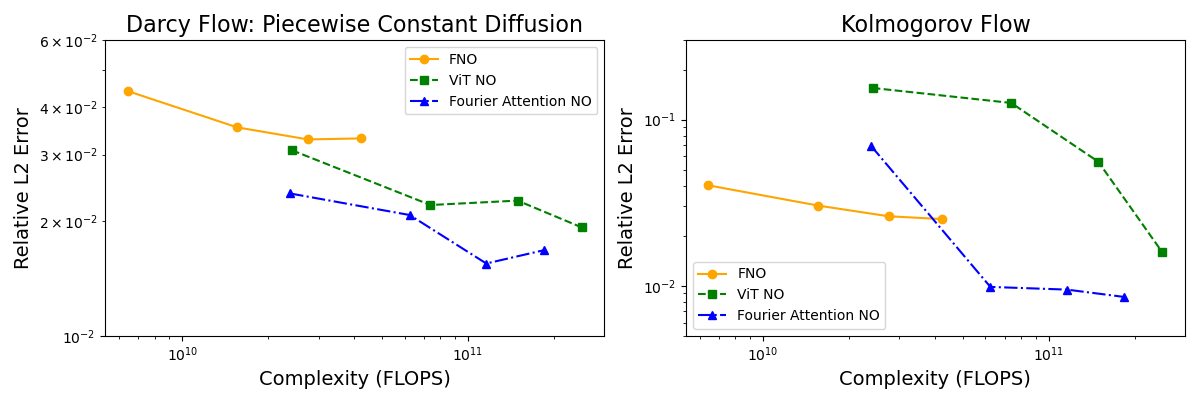
| Architecture | Darcy Flow | Darcy Flow | Kolmogorov Flow |
|---|---|---|---|
| Lognormal Input | Piecewise Constant Input | ||
| ViT NO | |||
| FANO | |||
| FNO |
6.2.2 Darcy Flow
We consider the linear, second-order elliptic PDE defined on the unit square
| (Darcy Flow) | ||||||
which is the steady-state of the 2D Darcy flow equation. The equation is equipped with Dirichlet boundary conditions and is well-posed when the diffusion coefficient and the forcing function is . In this context, we will consider learning the nonlinear operator defined as
We consider two different inputs. In both experimental settings the forcing function is chosen as .
In the first the data points are sampled from the probability measure
where is a Gaussian measure with covariance operator defined as
where the Laplacian is equipped with zero Neumann boundary conditions and viewed as acting between spaces of spatially mean-zero functions, and is the exponential function. We hence refer to the data inputs as being lognormal. In the second setting are sampled from the probability measure
where the covariance operator is defined as before and
We hence refer to the data inputs as being piecewise constant.
In the context of the lognormal experimental setting, we investigate a scenario with low resolution training samples, for which pointwise attention and hence the transformer neural operator from Subsection 4.2 is suitable, and a high resolution scenario where patching becomes necessary for application of the patched-based architectures of Subsections 4.3 and 4.4.
For the low resolution setting, we train the FNO and transformer neural operator architectures using independent samples of resolution , we use samples for validation and samples for testing. The Fourier neural operator is parametrized by Fourier modes in each dimension and channel width of ; the model is trained using a batch size of and learning rate of . On the other hand, the transformer neural operator is parametrized by channels in the encoder and is trained using a batch size of and learning rate of . On this problem we train both neural operators using the relative loss.
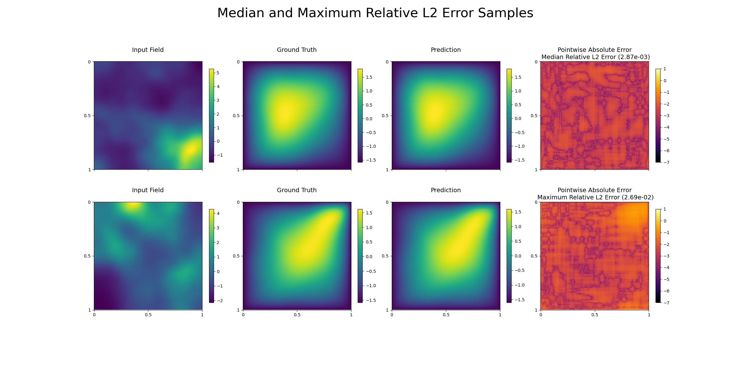
For the high resolution setting, we train the FNO, ViT neural operator and Fourier attention neural operator architectures using independent samples of resolution ; we use samples for validation and samples for testing. The Fourier neural operator is again parametrized by Fourier modes in each dimension and channel width of ; the model is trained using a batch size of and learning rate of . Both the ViT neural operator and Fourier attention neural operator are parametrized by channels in the transformer encoder. The integral operator in the ViT NO is parametrized by Fourier modes in each dimension while the integral operators appearing in the Fourier attention neural operator are parametrized by Fourier modes in each dimension. Both architectures employ a final spectral convolution layer (see Remark 21) that is parametrized by Fourier modes in each dimension. Both of these neural operators are trained using a batch size of and learning rate of . On this problem we train all the neural operators with the relative loss. Figure 11 displays the high resolution test results obtained by applying the Fourier attention neural operator.
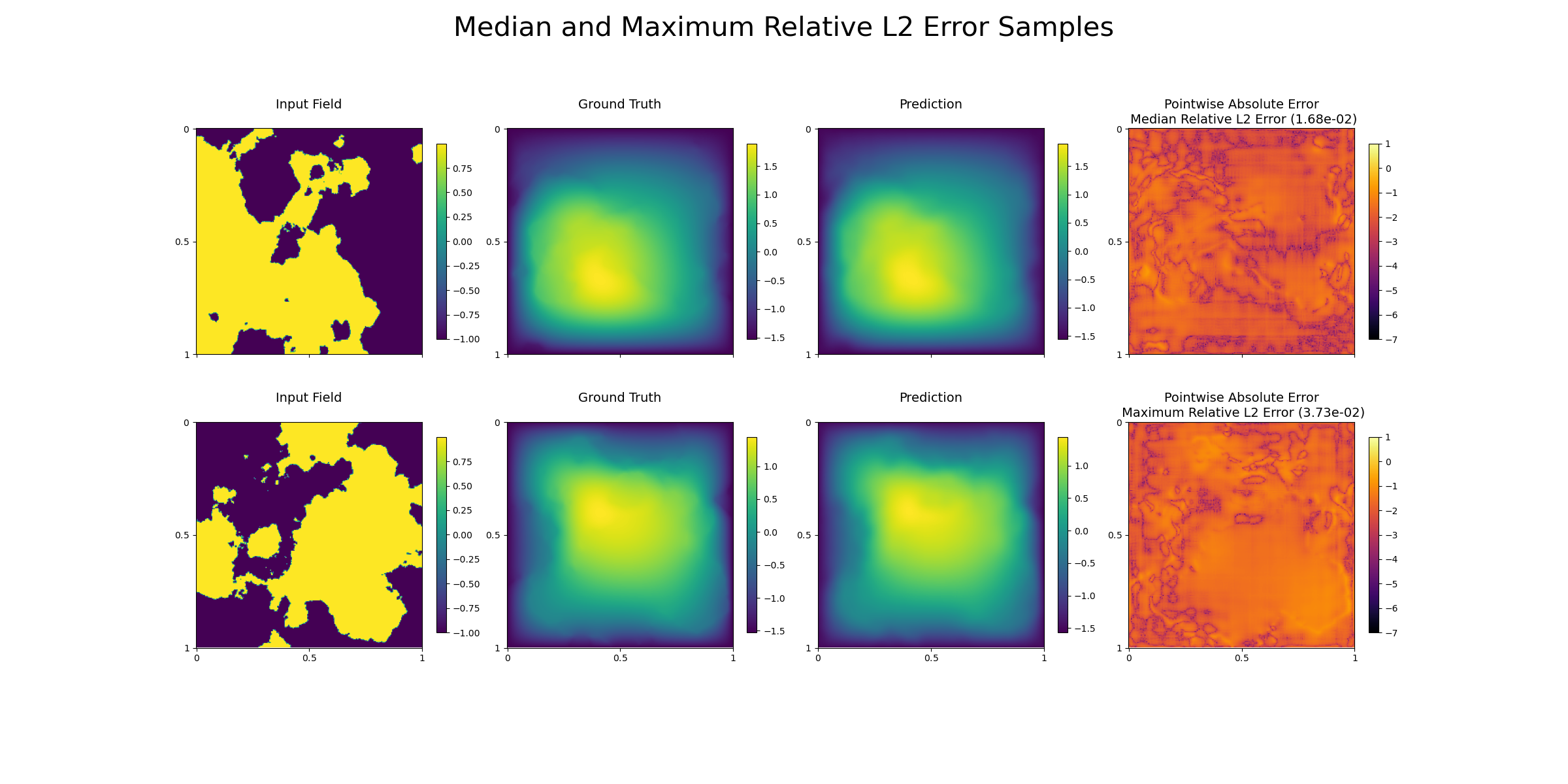
In the context of the piecewise constant experimental setting, we train the FNO, ViT neural operator and Fourier attention neural operator architectures using independent samples of resolution , we use samples for validation and samples for testing. The Fourier neural operator is again parametrized by Fourier modes in each dimension and channel width of ; the model is trained using a batch size of and learning rate of . Both the ViT neural operator and Fourier attention neural operator are parametrized by channels in the transformer encoder. The integral operator in the ViT NO is parametrized by Fourier modes in each dimension while the integral operators appearing in the Fourier attention neural operator are parametrized by Fourier modes in each dimension. Both architectures employ a final spectral convolution layer (see Remark 21) that is parametrized by Fourier modes in each dimension. Both of these neural operators are trained using a batch size of and learning rate of . On this problem we train all the neural operators with the relative loss. Figure 12 displays the high resolution test results obtained by applying the Fourier attention neural operator.
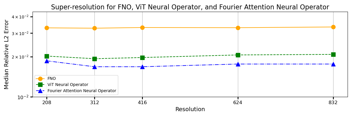
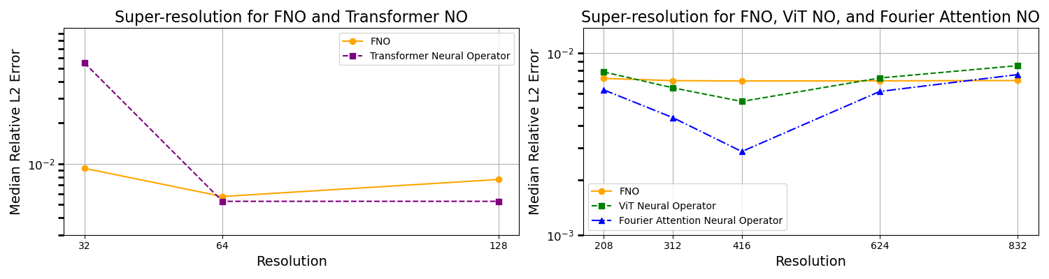
In Figures 13 and 14 we display the results of applying the neural operator architectures for the lognormal and piecewise input settings, respectively, to test samples of different resolutions than the one used for training. The results demonstrate the zero-shot generalization to different resolutions capability of the transformer neural operator architectures, which does not require retraining of the models. In the lognormal setting the FNO exhibits invariance to discretization that is more stable to changing resolution than are the ViT neural operator and the Fourier attention neural operator.
6.2.3 Kolmogorov Flow
We consider the two-dimensional Navier-Stokes equation for a viscous, incompressible fluid,
| (KF) | ||||||
where denotes the velocity, the pressure and the kinematic viscosity. The particular choice of forcing function leads to a particular example of a Kolmogorov flow. We equip the domain with periodic boundary conditions. We assume
The dot on denotes the space of spatially mean-zero functions. The vorticity is defined as and the stream function as the solution to the Poisson equation . Existence of the semigroup is shown in Temam (2012, Theorem 2.1). We generate the data by solving (KF) in vorticity-streamfunction form by applying the pseudo-spectral split step method from Chandler and Kerswell (2013). In our experimental set-up and are chosen. Random initial conditions are sampled from the Gaussian measure where the covariance operator is given by
where the Laplacian is equipped with periodic boundary conditions on , and viewed as acting between spaces of spatially mean-zero functions. The input output-data pairs for the Kolmogorov flow experiment are given by
for being i.i.d. samples. Indeed, given any we aim to approximate the nonlinear operator defined by
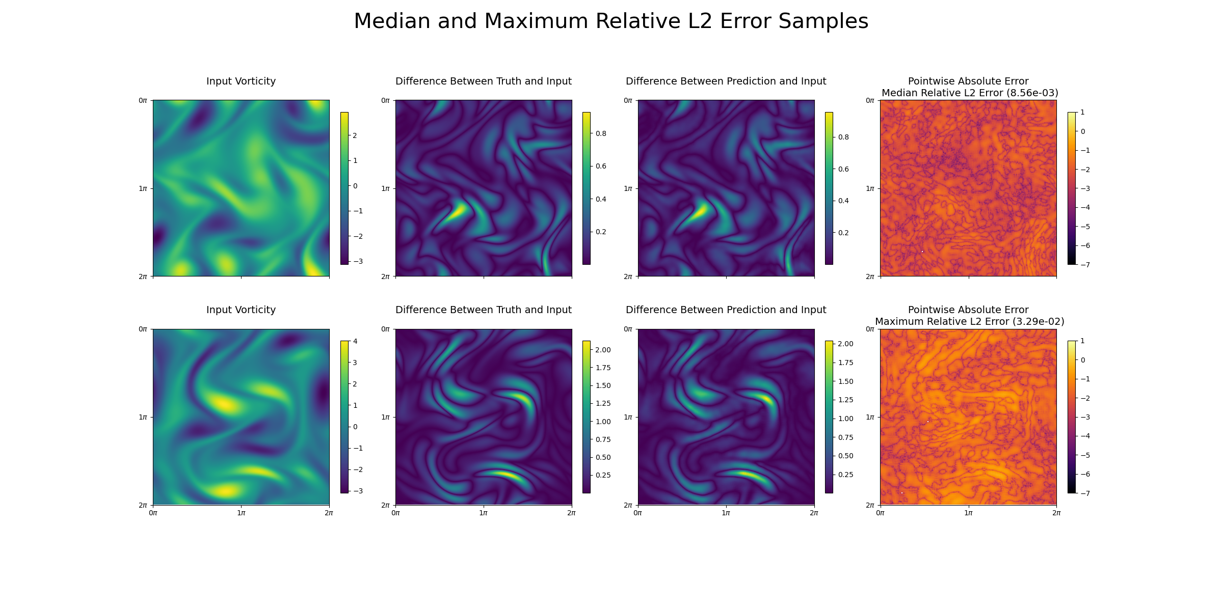
In our experimental setting, we set and . We train the FNO, ViT neural operator and Fourier attention neural operator architectures on this problem using independent samples of resolution , samples for validation and samples for testing. The Fourier neural operator is parametrized by Fourier modes in each dimension and channel width of ; the model is trained using a batch size of and learning rate of . Both the ViT neural operator and Fourier attention neural operator are parametrized by channels in the transformer encoder. The integral operator in the ViT NO is parametrized by Fourier modes in each dimension while the integral operators appearing in the Fourier attention neural operator are parametrized by Fourier modes in each dimension. Both architectures employ a final spectral convolution layer (Remark 21) that is parametrized by Fourier modes in each dimension. Both of these neural operators are trained using a batch size of and learning rate of . On this problem we train all the neural operators with the relative loss. Figure 15 displays the test results using the Fourier attention neural operators.
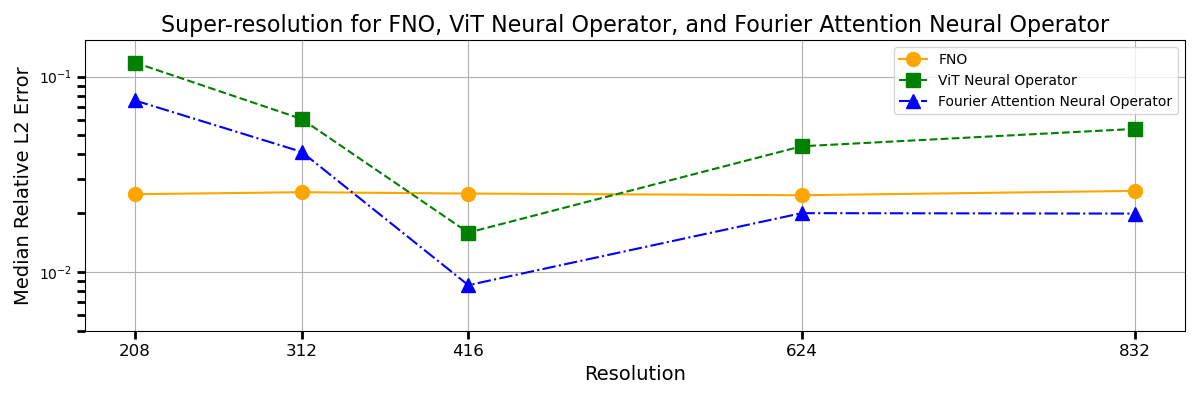
In Figure 16 we display the results of applying the three architectures to test samples of resolutions different to the training resolution. The results demonstrate the zero-shot generalization capability of the three neural operator architectures to different discretizations, which does not require retraining of the models. Again we note that FNO exhibits invariance to discretization that is more stable to changing resolution than the methods introduced here; but for all the neural operators it is nonetheless clear that intrinsic properties of the continuum limit are learned and may be transferred between discretizations.
A few additional considerations are in order. The mode truncation employed in the Fourier neural operator make the architecture computationally efficient but yields an over-smoothing effect that is not suitable for problems at high resolutions, where high frequency detail is prominent. Attention-based neural operators offer a possible solution to this issue, as demonstrated by the performance of the transformer neural operators proposed when applied to the PDE operator learning problems considered, which involve rough diffusion coefficients and rough initial conditions. On the other hand, patching leads to more efficient attention-based neural operators, but also introduces possible discontinuities at patch-intersections. This issue has been observed to be resolved in the large data regime. The residual spectral convolution layers employed ameliorate the discontinuities that are visible in pointwise error plots, but have a negligible effect on relative error in training and testing. This property constitutes an inherent limitation of patching and highlights the need for more suitable efficient attention mechanisms. Furthermore, it is observed that in some experimental settings the patching-based neural operators exhibit worse stability to changing resolution than FNO. This is likely due to the effect of patching which may then be further amplified for FANO due to the application of a higher number of FFT applications to non-periodic domains. Such issues could potentially be overcome using periodic extensions for Fourier-based parametrizations or other kinds of parametrizations for the nonlocal operations, or could be further improved by fine-tuning.
7 Conclusions
In this work we have introduced a continuum formulation of the attention mechanism from the seminal work Vaswani et al. (2017). Our continuum formulation can be used to design transformer neural operators. Indeed, this continuum formulation leads to discretization invariant implementations of attention and schemes that exhibit zero-shot generalization to different resolutions. In the first result of its kind for transformers, the resulting neural operator architecture mapping between infinite-dimensional spaces of functions is shown to be a universal approximator of continuous functions and functions of Sobolev regularity defined over a compact domain. We extend the continuum formulation to patched attention, which makes it possible to design efficient transformer neural operators. To this end, we introduce a neural operator analogue of the vision transformer Dosovitskiy et al. (2021) and a more expressive architecture, the Fourier attention neural operator. Through a cost-accuracy analysis, we demonstrate the power of the methodology in the context of high-resolution operator learning problems.
Acknowledgments and Disclosure of Funding
AMS is supported by a Department of Defense Vannevar Bush Faculty Fellowship; this funding also supports EC and partly supported MEL. In addition, AMS and EC are supported by the SciAI Center, funded by the Office of Naval Research (ONR), under Grant Number N00014-23-1-2729. NBK is grateful to the Nvidia Corporation for support through full-time employment. MEL is supported by funding from the Eric and Wendy Schmidt Center at the Broad Institute of MIT and Harvard.
We thank Théo Bourdais, Matthieu Darcy, Miguel Liu-Schiaffini, Georgia Gkioxari, Sabera Talukder, Zihui Wu, and Zongyi Li for helpful discussions and feedback.
Appendix A Proofs of Approximation Theorems
A.1 Proof of Self-Attention Approximation Theorem
We introduce the following auxiliary result that we will apply to prove Theorem 6.
Lemma 25
Let be a bounded open set and let be an i.i.d. sequence. If then, with the expectation taken over the data ,
Proof Notice that, for any ,
Hence, by expanding the square, we can observe that
Bounding in , and noting that it is a continuous function, gives
The result follows by Jensen’s inequality.
As part of the proof of Theorem 6, we first show that the the self-attention operator is a mapping of the form and hence .
Lemma 26
Let , then it holds that . Furthermore, for it holds that .
Proof The result follows readily from the fact that is a probability density function. For completeness, we show the boundedness of the normalization constant of the function . Indeed we note that,
for some constant . From definition, it is clear that
hence is indeed a valid probability density function. It hence follows that
hence . Similarly, it follows that
. We note that the continuity of is preserved by under the continuity of the inner product in its first argument and the continuity of the exponential.
We are now ready to establish the full result of Theorem 6 which states that
with the expectation taken over i.i.d. sequences .
Proof [Proof of Theorem 6] Before commencing the proof, we first establish useful shorthand notation. Letting we define,
for all and . For we also define
and
for any and any . We set and . Given this notation, to prove the result we must show
| (43) |
for any . We divide the proof in the following key steps. We first show that for fixed , it holds that
| (44) |
for any . By using compactness and applying the Arzelà-Ascoli theorem, we then show that
| (45) |
for any . We then use the compactness of and continuity of the mappings and to deduce the result given by (43). We now focus on establishing (44). Since is bounded, there exists a constant such that,
Therefore, we have
where . Clearly,
Notice that, since , we have . It follows that
Similarly,
Applying Lemma 25, for fixed we find that
| (46a) | ||||
| (46b) | ||||
Setting and , from (46a) we deduce that
| (47) |
for any . We now proceed to the second step of the proof, i.e. showing that (45) holds. Using similar reasoning as before, we notice that
| (48a) | ||||
| (48b) | ||||
hence the sequence is uniformly bounded in . Now, for fixed the sequence is also uniformly equicontinuous with probability 1 over the choice . Indeed, we note that
| (49a) | ||||
| (49b) | ||||
| (49c) | ||||
The result then follows from the uniform continuity of and in their first arguments, due to the compactness of . Therefore, since is compact, by the Arzelà–Ascoli theorem there exists a subsequence of indices such that converges in to some . Since,
by uniqueness of limits, it is readily observed that . Therefore, since the limit is independent of the subsequence, it holds that
for any . We now turn our attention to establishing (43). By reasoning as before and by using the continuity of the exponential and the inner product in its first argument, it is straightforward to show that as mappings of the form and where is compact, and are continuous and hence the sequence is uniformly equicontinuous. Therefore, we can find moduli of continuity such that
for any and . Fix . Since is compact, we can find a number and functions such that, for any , there exists such that
Furthermore, we can find a number such that, for any , we have, for all ,
It follows by triangle inequality that
Therefore the result follows since the argument is uniform over all .
A.2 Proof of Cross-Attention Approximation Theorem
We make straightforward modifications to Lemmas 25, 28 and to the proof of Theorem 6 in order to establish Theorem 12.
Lemma 27
Let and be bounded open sets and . Then
with the expectation taken over i.i.d. sequences .
Proof Notice that, for any ,
Hence, by expanding the square, we can observe that
Bounding in , and noting that it is a continuous function, gives
The result follows by Jensen’s inequality.
As part of the proof of Theorem 12, we first show that the the cross-attention operator is a mapping of the form and hence .
Lemma 28
Let , then it holds that . Furthermore, for it holds that .
Proof The result follows readily from the fact that is a probability density function. For completeness, we show the boundedness of the normalization constant of the function . Indeed we note that,
for some constant . From definition, it is clear that
hence is indeed a valid probability density function. It hence follows that
hence . Similarly, it follows that
. We note that the continuity is preserved by under the continuity of the inner product in its first argument and the continuity of the exponential.
We are now ready to establish the full result of Theorem 12 which states that
with the expectation taken over i.i.d. sequences .
Proof [Proof of Theorem 12] Before commencing the proof, we first establish useful shorthand notation. Letting we define,
for all and . For we also define
and
for any and any . We set and . Given this notation, to prove the result we must show
| (50) |
for any . We divide the proof in the following key steps. We first show that for fixed , it holds that
| (51) |
for any . By using compactness and applying the Arzelà-Ascoli theorem, we then show that for
| (52) |
for any . We then use the compactness of and continuity of the mappings and to deduce the result given by (50). We now focus on establishing (51). Since is bounded, there exists a constant such that,
Therefore, we have
where . Clearly, it holds that
Notice that, since , we have . It follows that
Similarly,
Applying Lemma 27, we find
| (53a) | ||||
| (53b) | ||||
Setting and , from (53a) we deduce that for it holds that
| (54) |
for any . We now proceed to the second step of the proof, i.e. showing that (52) holds. Using similar reasoning as before, we notice that
| (55a) | ||||
| (55b) | ||||
hence the sequence is uniformly bounded in . Now, for fixed the sequence is also uniformly equicontinuous with probability 1 over the choice . Indeed, we note that
| (56a) | ||||
| (56b) | ||||
| (56c) | ||||
The result then follows from the uniform continuity of and in their first arguments, due to the compactness of . Therefore, since is compact, by the Arzelà–Ascoli theorem there exists a subsequence of indices such that converges in to some . Since,
by uniqueness of limits, it is readily observed that . Therefore, since the limit is independent of the subsequence, for fixed it holds that
for any . We now turn our attention to establishing (50). By reasoning as before and by using the continuity of the exponential and of the inner product on the product space, it is straightforward to show that as mappings of the form and where is compact, and are continuous and hence the sequence is uniformly equicontinuous. Therefore, we can find moduli of continuity such that
for any and . Fix . Since is compact, we can find a number and functions such that, for any , there exists such that
Furthermore, we can find a number such that, for any , we have, for all ,
It follows by triangle inequality that
Therefore the result follows since our argument is uniform over all .
Appendix B Transformer Neural Operators: The Discrete Setting
We describe how the transformer neural operators described in Section 4 are implemented in the discrete setting. Namely, in practice we will have access to evaluations of the input function at a finite set of discretization points . To highlight how the neural operator methodology is applied in practical settings it is useful, abusing notation, to view the input to the neural operators as . In order to distinguish between functions in , and discrete representations of these functions at a finite set of grid points, in this section we use different fonts for a function and its discrete analogue . We highlight that in practice, it is of interest to apply approximations of the attention operators and defined on the continuum, to . Through an abuse of notation, we will write to denote the finite-dimensional approximation of acting on matrices, and similarly for and
In Subsection B.1 we describe the transformer neural operator in the discrete setting, in Subsection B.2 the vision transformer neural operator and in Subsection B.3 the Fourier attention neural operator.
B.1 Transformer Neural Operator
In this section, we describe how the transformer neural operator from Subsection 4.2 is implemented in the discrete setting. The input to the model is therefore a tensor , which is then concatenated with the discretization points , to form the tensor . The learnable linear transformation then acts on to yield
which is then fed through the transformer encoder. In practice we solve the recurrence relation in (10) on a finite set of grid points that arise naturally from the discrete input . The multi-head attention operator is defined by the application of the linear transformation to the concatenation of self-attention operations. The concatenation of the outputs of the self-attention operations results in a tensor, so that
| (57) |
for any . We recall that the self-attention operator in question, , is defined in Definition 5 for functions. In the discrete setting, where , we compute the expectation and the integral arising from the normalization constant using the following trapezoidal approximations:
| (58) |
for any , with
| (59) |
where by we have denoted the ’th row of the matrix , and similarly for . In equations (58) and (59) denotes
for , where is the ’th component of the vector . This trapezoidal approximation allows for a mathematically consistent implementation of attention for irregularly sampled data, as demonstrated in Section 6.
The linear transformations are applied pointwise. It is also straightforward to apply the definitions for in (16) and in (18) to the finite representation of as both involve pointwise linear transformations. We observe that the recurrence relation (10) is compatible with varying domain discretization lengths , and will produce an output of dimension matching the input . The resulting tensor is then projected to the output dimension by applying the learnable linear transformation , so that the output of the architecture is defined as
B.2 Vision Transformer Neural Operator
In this section, we describe how the transformer neural operator from Subsection 4.3 is implemented in the discrete setting. In practice, we will have access to a discretization of the domain containing points and evaluations of the function at these points; the resolution of the input will be determined by . The input to the model will therefore be a tensor . The input is first concatenated with the discretization points , to form the tensor . Denoting by the resolution of each patch, application of the reshaping operator results in
Following Definition 20 and the subsequent discussion, the nonlocal linear operator is implemented as
| (60) |
for any , where we have made explicit the dependence on to highlight the learnable components in the implementation. The FFT is computed on the dimensions so that the resulting tensor is of the form . Since is convolved with a function that possess only Fourier modes, the higher Fourier modes may be truncated so that one may consider . The learnable tensor is and the operation in Fourier space is defined as
| (61) |
for . The inverse FFT is then applied along the dimensions . The resulting tensor defined as is then fed through the transformer encoder .
The multi-head attention is based on the self-attention operator acting on functions from Definition 14. While the expectation is computed with respect to a probability measure on the patch sequence, hence inducing a discrete probability mass function, the discretization of the domain introduces the need to approximate the inner product appearing in Definition 13. We resort to an approximation of the integral given by
| (62a) | ||||
| (62b) | ||||
where we have denoted by the volume of the th cell. We recall that in this case the linear operators are pointwise local operators hence they admit finite dimensional representations , for . In the case of uniform patching and uniform discretization of the domain of size , which is the setting we experiment with, the approximation reduces to the approximation of the integral of the form
| (63) |
The multi-head attention operator is thus defined by the application of the linear transformation to the concatenation of self-attention operations defined by the approximations above. The concatenation of the outputs of the self-attention operations results in a tensor, so that
| (64) |
for any . The linear transformations are applied pointwise. The layer normalization operator is applied as defined in (24) to every point in every patch so that .
The operator is applied so that , for any . Indeed, in this finite-dimensional setting is defined as
| (65) |
for any , where is a nonlinear activation function are learnable local linear operators and are learnable in the last dimension.
After computing the recurrence for as described in Equation 10, a reshaping operator is applied to the resulting tensor so that
| (66) |
for any . A pointwise linear transformation is then applied according to
| (67) |
for any . Following Remark 21, an additional convolution in frequency space may be applied in residual form, where application of the nonlocal integral operator follows Definition 20 and the subsequent discussion. To this end, the operation in frequency space is defined similarly to (61) and the learnable tensor is of the form
B.3 Fourier Attention Neural Operator
In this section, we describe how the transformer neural operator from Subsection 4.4 is implemented in the discrete setting. In practice, we consider a discretization of the domain containing points and evaluations of the function at these points; the resolution of the input is defined by . The input to the model is hence a tensor . The input is concatenated with the discretization points , to form the tensor . Denoting by the resolution of each patch, application of the reshaping operator results in
The learnable linear transformation is then applied as a map
The resulting tensor is then fed through the transformer encoder
In the recurrence relation that defines the encoder, is the multi-head attention operator as defined in equation (11). In this setting, letting denote the number of attention heads, the multi-head attention operator is parametrized by learnable linear integral operators , , and for . Following Definition 20 and the subsequent discussion we implement the linear integral operators as
| (68a) | ||||
| (68b) | ||||
| (68c) | ||||
for and any , where we have made explicit the dependence on to highlight the learnable components in the implementation. In (68) the FFT is computed on the so that the resulting tensor . Since is a function that possess only Fourier modes, the higher Fourier modes may be truncated so that one may consider . The learnable tensors are of dimension for , and the operation in Fourier space is defined as
| (69) |
for any and . The inverse FFT is computed along the dimensions so that for . We recall that in this case the self-attention operator is defined according to Definition 14. While the expectation is computed with respect to a probability measure on the patch sequence, hence inducing a discrete probability mass function, the discretization of the domain introduces the need to approximate the inner product appearing in Definition 13. We resort to an approximation of the integral given by (62) and (63). The multi-head attention operator is thus defined by the application of the linear transformation to the concatenation of self-attention operations. The concatenation of the outputs of the self-attention operations results in a tensor, so that
| (70) |
for any . The linear transformations are applied pointwise. The layer normalization operator is applied as defined in (16) to every point in every patch so that . Finally, the operator is parametrized and applied as in (65) so that , for any .
A reshaping operator to the tensor resulting from the transformer encoder iteration as in Equation 66. A pointwise linear transformation is then applied as in Equation 67. Again, following Remark 21, an additional convolution in frequency space may be applied in residual form, where application of the nonlocal integral operator follows Definition 20 and the subsequent discussion. To this end, the operation in frequency space is defined similarly to (61) and the learnable tensor is of the form
Appendix C Complexity of the Transformer Neural Operators
We summarize the expressions for the parameter complexity and evaluation cost (measured in floating point operations, FLOPS) of the neural operators from Section 4 and the Fourier neural operator (FNO) from Li et al. (2021). These are provided in Tables 4 and 5, respectively. In Subsection C.1 and C.2 we provide further details for the computations of the parameter and evaluation cost complexities, respectively.
C.1 Parameter Complexity
| Architecture | Parameter Complexity |
|---|---|
| FNO | |
| Transformer NO | |
| ViT NO | |
| FANO |
C.2 Evaluation Cost
We note that a matrix vector product for has cost . We approximate the cost of computing the FFT of a vector in as (Hoop et al., 2022). We approximate the cost of the two-dimensional real FFT, used in implementation, by where is the total number of grid points. Assuming that the grid is of size for an even integer, 1d FFTs are first computed for each row. The real FFT requires column 1d FFTs, hence the complexity.
| Architecture | Evaluation Cost |
|---|---|
| FNO | |
| Transformer NO | |
| ViT NO | |
| FANO |
References
- Bahdanau et al. (2014) Dzmitry Bahdanau, Kyunghyun Cho, and Yoshua Bengio. Neural machine translation by jointly learning to align and translate. CoRR, abs/1409.0473, 2014.
- Bi et al. (2023) Kaifeng Bi, Lingxi Xie, Hengheng Zhang, Xin Chen, Xiaotao Gu, and Qi Tian. Accurate medium-range global weather forecasting with 3d neural networks. Nature, 619:1–6, 07 2023.
- Cao (2021) Shuhao Cao. Choose a transformer: Fourier or galerkin. In M. Ranzato, A. Beygelzimer, Y. Dauphin, P.S. Liang, and J. Wortman Vaughan, editors, Advances in Neural Information Processing Systems, volume 34, pages 24924–24940. Curran Associates, Inc., 2021.
- Chandler and Kerswell (2013) Gary J. Chandler and Rich R. Kerswell. Invariant recurrent solutions embedded in a turbulent two-dimensional kolmogorov flow. Journal of Fluid Mechanics, 722:554–595, 2013. doi: 10.1017/jfm.2013.122.
- Chattopadhyay et al. (2022) A. Chattopadhyay, M. Mustafa, P. Hassanzadeh, E. Bach, and K. Kashinath. Towards physics-inspired data-driven weather forecasting: integrating data assimilation with a deep spatial-transformer-based u-net in a case study with era5. Geoscientific Model Development, 15(5):2221–2237, 2022.
- Chen et al. (2017) Long Chen, Hanwang Zhang, Jun Xiao, Liqiang Nie, Jian Shao, Wei Liu, and Tat-Seng Chua. Sca-cnn: Spatial and channel-wise attention in convolutional networks for image captioning. In Proceedings of the IEEE conference on computer vision and pattern recognition, pages 5659–5667, 2017.
- Cheng et al. (2023) Sibo Cheng, César Quilodrán-Casas, Said Ouala, Alban Farchi, Che Liu, Pierre Tandeo, Ronan Fablet, Didier Lucor, Bertrand Iooss, Julien Brajard, Dunhui Xiao, Tijana Janjic, Weiping Ding, Yike Guo, Alberto Carrassi, Marc Bocquet, and Rossella Arcucci. Machine learning with data assimilation and uncertainty quantification for dynamical systems: A review. IEEE/CAA Journal of Automatica Sinica, 10(6):1361–1387, 2023.
- Chung et al. (2014) Junyoung Chung, Caglar Gulcehre, Kyunghyun Cho, and Yoshua Bengio. Empirical evaluation of gated recurrent neural networks on sequence modeling. In Neural Information Processing Systems 2014 Workshop on Deep Learning, December 2014, 2014.
- Dosovitskiy et al. (2021) Alexey Dosovitskiy, Lucas Beyer, Alexander Kolesnikov, Dirk Weissenborn, Xiaohua Zhai, Thomas Unterthiner, Mostafa Dehghani, Matthias Minderer, Georg Heigold, Sylvain Gelly, Jakob Uszkoreit, and Neil Houlsby. An image is worth 16x16 words: Transformers for image recognition at scale. In 9th International Conference on Learning Representations, ICLR 2021, Virtual Event, Austria, May 3-7, 2021, 2021.
- Geshkovski et al. (2023) Borjan Geshkovski, Cyril Letrouit, Yury Polyanskiy, and Philippe Rigollet. The emergence of clusters in self-attention dynamics. arXiv preprint, arXiv:2305.05465, 2023.
- Guibas et al. (2022) John Guibas, Morteza Mardani, Zongyi Li, Andrew Tao, Anima Anandkumar, and Bryan Catanzaro. Efficient token mixing for transformers via adaptive fourier neural operators. In International Conference on Learning Representations, 2022.
- Hao et al. (2023) Zhongkai Hao, Zhengyi Wang, Hang Su, Chengyang Ying, Yinpeng Dong, Songming Liu, Ze Cheng, Jian Song, and Jun Zhu. Gnot: A general neural operator transformer for operator learning. In Proceedings of the 40th International Conference on Machine Learning, ICML’23. JMLR.org, 2023.
- Hayden et al. (2011) Kevin Hayden, Eric Olson, and Edriss S. Titi. Discrete data assimilation in the lorenz and 2d navier–stokes equations. Physica D: Nonlinear Phenomena, 240(18):1416–1425, 2011.
- Hochreiter and Schmidhuber (1997) Sepp Hochreiter and Jürgen Schmidhuber. Long Short-Term Memory. Neural Computation, 9(8):1735–1780, 11 1997.
- Hoop et al. (2022) Maarten V. de Hoop, Daniel Zhengyu Huang, Elizabeth Qian, and Andrew M. Stuart. The cost-accuracy trade-off in operator learning with neural networks. Journal of Machine Learning, 1(3):299–341, 2022. ISSN 2790-2048.
- Kaplan et al. (2020) Jared Kaplan, Sam McCandlish, Tom Henighan, Tom B. Brown, Benjamin Chess, Rewon Child, Scott Gray, Alec Radford, Jeff Wu, and Dario Amodei. Scaling laws for neural language models. arXiv preprint, arXiv:2001.08361, 2020.
- Kovachki et al. (2023) Nikola Kovachki, Zongyi Li, Burigede Liu, Kamyar Azizzadenesheli, Kaushik Bhattacharya, Andrew Stuart, and Anima Anandkumar. Neural operator: Learning maps between function spaces with applications to pdes. Journal of Machine Learning Research, 24(89):1–97, 2023.
- Lanthaler et al. (2023) Samuel Lanthaler, Zongyi Li, and Andrew M. Stuart. The nonlocal neural operator: Universal approximation. arXiv preprint, arXiv:2304.13221, 2023.
- Li et al. (2023) Zijie Li, Kazem Meidani, and Amir Barati Farimani. Transformer for partial differential equations’ operator learning. Transactions on Machine Learning Research, 2023. ISSN 2835-8856.
- Li et al. (2021) Zongyi Li, Nikola Borislavov Kovachki, Kamyar Azizzadenesheli, Burigede liu, Kaushik Bhattacharya, Andrew Stuart, and Anima Anandkumar. Fourier neural operator for parametric partial differential equations. In International Conference on Learning Representations, 2021.
- Liu et al. (2021) Z. Liu, Y. Lin, Y. Cao, H. Hu, Y. Wei, Z. Zhang, S. Lin, and B. Guo. Swin transformer: Hierarchical vision transformer using shifted windows. In 2021 IEEE/CVF International Conference on Computer Vision (ICCV), pages 9992–10002, Los Alamitos, CA, USA, 10 2021. IEEE Computer Society.
- Lorenz (1963) Edward N Lorenz. Deterministic nonperiodic flow. Journal of atmospheric sciences, 20(2):130–141, 1963.
- Martins et al. (2020) André Martins, António Farinhas, Marcos Treviso, Vlad Niculae, Pedro Aguiar, and Mario Figueiredo. Sparse and continuous attention mechanisms. In H. Larochelle, M. Ranzato, R. Hadsell, M.F. Balcan, and H. Lin, editors, Advances in Neural Information Processing Systems, volume 33, pages 20989–21001. Curran Associates, Inc., 2020.
- Moreno et al. (2022) Alexander Moreno, Zhenke Wu, Supriya Nagesh, Walter Dempsey, and James M Rehg. Kernel multimodal continuous attention. In S. Koyejo, S. Mohamed, A. Agarwal, D. Belgrave, K. Cho, and A. Oh, editors, Advances in Neural Information Processing Systems, volume 35, pages 18046–18059. Curran Associates, Inc., 2022.
- Ovadia et al. (2023) Oded Ovadia, Adar Kahana, Panos Stinis, Eli Turkel, and George Em Karniadakis. Vito: Vision transformer-operator. arXiv preprint, arXiv:2303.08891, 2023.
- Pecora and Carroll (1990) Louis M. Pecora and Thomas L. Carroll. Synchronization in chaotic systems. Phys. Rev. Lett., 64:821–824, 2 1990.
- Pinkus (1999) Allan Pinkus. Approximation theory of the mlp model in neural networks. Acta Numerica, 8:143–195, 1999.
- Rahman et al. (2024) Md Ashiqur Rahman, Robert Joseph George, Mogab Elleithy, Daniel Leibovici, Zongyi Li, Boris Bonev, Colin White, Julius Berner, Raymond A. Yeh, Jean Kossaifi, Kamyar Azizzadenesheli, and Anima Anandkumar. Pretraining codomain attention neural operators for solving multiphysics pdes. arXiv preprint, arXiv:2403.12553, 2024.
- Ronneberger et al. (2015) Olaf Ronneberger, Philipp Fischer, and Thomas Brox. U-net: Convolutional networks for biomedical image segmentation. In Nassir Navab, Joachim Hornegger, William M. Wells, and Alejandro F. Frangi, editors, Medical Image Computing and Computer-Assisted Intervention – MICCAI 2015, pages 234–241, Cham, 2015. Springer International Publishing. ISBN 978-3-319-24574-4.
- Sanz-Alonso et al. (2023) Daniel Sanz-Alonso, Andrew Stuart, and Armeen Taeb. Inverse Problems and Data Assimilation. London Mathematical Society Student Texts. Cambridge University Press, 2023.
- Temam (2012) R. Temam. Infinite-Dimensional Dynamical Systems in Mechanics and Physics. Applied Mathematical Sciences. Springer New York, 2012. ISBN 9781468403138.
- Tsai et al. (2019) Yao-Hung Hubert Tsai, Shaojie Bai, Makoto Yamada, Louis-Philippe Morency, and Ruslan Salakhutdinov. Transformer dissection: An unified understanding for transformer’s attention via the lens of kernel. In Kentaro Inui, Jing Jiang, Vincent Ng, and Xiaojun Wan, editors, Proceedings of the 2019 Conference on Empirical Methods in Natural Language Processing and the 9th International Joint Conference on Natural Language Processing (EMNLP-IJCNLP), pages 4344–4353, Hong Kong, China, November 2019. Association for Computational Linguistics.
- Vaswani et al. (2017) Ashish Vaswani, Noam Shazeer, Niki Parmar, Jakob Uszkoreit, Llion Jones, Aidan N Gomez, Ł ukasz Kaiser, and Illia Polosukhin. Attention is all you need. In I. Guyon, U. Von Luxburg, S. Bengio, H. Wallach, R. Fergus, S. Vishwanathan, and R. Garnett, editors, Advances in Neural Information Processing Systems, volume 30. Curran Associates, Inc., 2017.
- Wen et al. (2023) Qingsong Wen, Tian Zhou, Chaoli Zhang, Weiqi Chen, Ziqing Ma, Junchi Yan, and Liang Sun. Transformers in time series: A survey. In International Joint Conference on Artificial Intelligence(IJCAI), 2023.
- Wright and Gonzalez (2021) Matthew A Wright and Joseph E. Gonzalez. Transformers are deep infinite-dimensional non-mercer binary kernel machines. arXiv preprint, arXiv:2106.01506, 2021.
- Yun et al. (2020) Chulhee Yun, Srinadh Bhojanapalli, Ankit Singh Rawat, Sashank Reddi, and Sanjiv Kumar. Are transformers universal approximators of sequence-to-sequence functions? In International Conference on Learning Representations, 2020.