Non-equilibrium cotunneling in interacting Josephson junctions
Abstract
We investigate non-equilibrium transport through interacting superconducting nanojunctions using a Liouville space approach. The formalism allows us to study finite gap effects, and to account for both quasiparticle and Cooper pair tunneling. With focus on the weak tunneling limit, we study the stationary dc and ac current up to second order (cotunneling) in the hybridization energy. We identify the characteristic virtual processes that yield the Andreev and Josephson current and obtain the dependence on the gate and bias voltage for the dc current, the critical current and the phase-dependent dissipative current. In particular, the critical current is characterized by regions in the stability diagram in which its sign changes from positive to negative, resulting in a multitude of transitions. The latter signal the interplay between strong interactions and tunneling at finite bias.
I Introduction
Advancements in nanostructure fabrication have allowed the manufacturing of increasingly smaller Josephson junctions. For mesoscopic and nano-sized junctions, genuine quantum mechanical effects often rule the transport properties of the device. Superconducting junctions based on quantum point contacts were among the first of such systems to be studied in detail [1, 2, 3]. For short weak links with few channels, multiple coherent Andreev reflections give rise to current-carrying Andreev bound states which can be employed to effectively characterize the properties of the Josephson current [4]. These ideas have been used extensively in recent years to investigate novel superconducting transport phenomena, such as the fractional Josephson effect in topological junctions [5, 6, 7], non-reciprocal transport [8, 9, 10], and multi-terminal junctions [11, 12].
As the size of the junction is decreased even further, Coulomb interaction effects between the strongly confined charge carriers becomes more important. Josephson junctions based on quantum dots (QDs), have been studied in detail both experimentally [13, 14, 15, 16, 17] and theoretically [18, 19, 20]. They have further received attention as a platform for quantum computation, in the form of Andreev spin qubits [21, 22]. The combination of superconducting correlations and electronic interactions yields a rich phenomenology [23, 24]. A hallmark of this interplay is the transition, occurring in QDs with odd occupancy. Here the sign of the equilibrium critical current changes as the junction’s ground state turns from a singlet to a doublet [25, 26, 27, 28, 29]. For strongly coupled QDs, Kondo correlations further affect the doublet and singlet phases [30, 31, 32, 33]. This work extends these results to a non-equilibrium situation. In particular, we show that a multitude of transitions can be observed in weakly coupled junctions, in a delicate interplay between interaction effects and Cooper pair tunneling at finite bias.
The Green’s function formalism is the method of choice for non-interacting junctions. While it has been extended to interacting systems via mean field [34, 35] and perturbative expansions [36, 37], the regime of interest for Josephson junctions often involves interaction strengths that lie beyond the applicability of these approximation schemes [38]. Alternatively, the tunnel coupling to the leads can be treated perturbatively while keeping the interaction exactly [39, 40, 41]. In order to perform this expansion systematically, a generalized master equation (GME) for the density operator can be employed [42, 43, 44], in which the distinct tunneling processes can be identified using diagrammatic techniques. This formalism can furthermore be extended to larger tunneling amplitudes via diagrammatic resummations [45, 46, 47] and renormalization group methods [48].
The GME approach has found applications in the study of QD-based Josephson junctions. This includes three-terminal junctions with one metallic lead which acts as a tunneling probe [49, 50, 51], Cooper pair splitters [52, 53, 54, 55] and Andreev bound state spectra [15, 56, 57]. Many of these works employ other approximations on top of weak coupling, such as the assumption of infinite gap or infinite interaction. The former, in particular, allows for resummation techniques that restore the Andreev bound state picture [58, 59, 60], and can even be extended to capture perturbatively the effect of the quasiparticles [61]. Recent works have employed fermionic duality to investigate the dynamics in the time domain of junctions with large gap superconductors [62, 63].
Non-equilibrium properties of Josephson junctions through interacting quantum dots have received a comparatively poor attention so far. This regime offers, nonetheless, a rich phenomenology [64, 65, 66, 67, 68, 69]. The finite bias properties of a carbon-nanotube based Josephson QD have been probed in a recent experiment by the measurement of the Josephson radiation [70] with intriguing unexplained features. This is the topic of the present work.
In the non-equilibrium case the GME approach is often used in a particle conserving framework of superconductivity [71], since it naturally allows to account for finite bias voltages across the junction [49, 67]. In a recent publication [72], some of us have employed the GME approach to investigate the interplay of a dc and an ac bias voltage on the transport characteristics of a Josephson quantum dot at finite gaps, temperature and interaction. In that study it was shown that, already in lowest order in the tunneling coupling, intriguing features may occur, such as an inversion of the dc-current due to the combination of the ac drive and a non-flat density of states.
Here we focus solely on the effects of a dc voltage bias on transport and fully include the first two non-vanishing orders in the tunnel coupling. We provide comprehensive numerical and analytical results for both the dc component of the current as well as its first harmonic in the ac Josephson frequency. For the latter, which provides the Josephson current out of equilibrium, we find two distinct contributions: the critical current, which remains finite at zero bias, and a phase-dependent dissipative term, sometimes referred to as the term [73, 74]. Knowledge of both allows us to evaluate the Josephson radiation, hence providing a direct benchmark to present cutting-edge experiments [75, 70].
As we shall see, accounting for the second order is fundamental, as the Josephson current is of this order for most situations. Inspection of the stability diagrams allows us to identify the relevant transport processes, being mediated solely by quasiparticles, Cooper pairs or a combination of both. For example, subgap features from thermally excited quasiparticles permeate the dc-component of the current. Elastic Cooper pair cotunneling is responsible for a phase of the critical current in the odd Coulomb diamond at low bias, extending results found for the zero bias case [39].
The manuscript is organized as follows. Section II introduces the model and the transport theory that we will employ throughout this work. In particular, in Section II.5 we show how the ac Josephson effect appears naturally in the system as a consequence of considering arbitrary coherences involving Cooper pairs. In Section III we introduce the perturbative scheme employed to calculate the steady state density operator and the current. In Section IV and Section V we present numerical results for the dc and ac components of the current and highlight their main features. Finally, in Section VI we summarize our results and provide an outlook for future research.
II Theoretical framework
II.1 Model Hamiltonian
We focus on the archetypal model of an interacting Josephson junction: the single impurity Anderson model (SIAM) with superconducting leads. The total Hamiltonian includes the contributions from the leads , the quantum dot , and the tunnel coupling between them . The last two are given respectively by
| (1) | ||||
| (2) |
Here, are annihilation (creation) operators of the dot with spin , while is the single particle energy of the dot, tunable via an electric gate with voltage . We choose in the following . Finally, is the Coulomb interaction. The tunneling process is characterized by spin conserving tunneling amplitudes for the transfer of a dot electron to lead , where it is described by annihilation (creation) fermionic operators with momentum and spin .
In order to account for charge transfer out of equilibrium, we treat the superconductors in a particle-conserving formulation [76, 77]. In this framework, the bare fermion operators can be written, employing the particle-conserving Bogoliubov-Valatin transformations, as
| (3) |
where for , respectively, and
| (4) | ||||
| (5) |
with the quasiparticle excitation energy for mode . Here, describes the single particle dispersion of the bare fermions measured from the chemical potential , is the superconducting order parameter, and . We take in this work without loss of generality. More importantly, we have employed the Bogoliubov operators which describe quasiparticle excitations, as well as Cooper pair operators which destroy or create a Cooper pair in the condensate [71]. Hence, the Bogoliubov-Valatin transformation conserves the total charge. The first term in Eq. 3 describes an electron-like excitation, while the second is associated with a hole-like excitation [78].
The quasiparticle states are characterized by the occupation of the fermionic modes, and the state of the Cooper pair condensate by the total number of Cooper pairs, which we denote by . With this, we can write an arbitrary state of lead as , with total number of electrons (Cooper pairs and quasiparticles) equal to . The effect of the Cooper pair operators on any such state is given by
| (6) |
Similarly, reduces by 1 and leaves the occupation of the quasiparticle states invariant. Employing this, we see that the Cooper pair and quasiparticle operators commute [79]
| (7) |
Moreover, the Cooper pair creation and annihilation operators satisfy
| (8) |
Assuming that the Cooper pair operators commute is a good approximation in the limit of large Cooper pair numbers and we do so from here onward.
Upon employing Eq. 3, we can divide the Hamiltonian for the leads into two contributions, The former describes the quasiparticle excitations and reads
| (9) | ||||
| (10) |
where is the chemical potential of lead , is the bias voltage and the coefficients satisfy . The latter contribution describes the Cooper pair condensate and has the form
| (11) |
Together with Eq. 6 and the corresponding equation for , it follows that
The Hamiltonian corresponds to a mean field approximation to the true Hamiltonian of the superconductor. By definition, the quasiparticles operators describe excitations on top of the ground state. Within the mean field approximation, the quasiparticle spectrum is assumed to be independent of the number of Cooper pairs in the ground state, yielding the commutation relations in Eq. 7. As a result of these relations, we find in the approximation of large Cooper pair numbers, but . The consequences and validity of the approximation will be further discussed in Section II.5. We anticipate that, since the quasiparticles are the only source of dissipation in the model, the dynamics of the Cooper pair sector is completely coherent and their time evolution is fully determined by the commutation with the Cooper pair Hamiltonian,
II.2 Transport theory
Interacting open quantum systems can be studied via a many-body generalized master equation (GME) based on the Nakajima-Zwanzig formalism [80, 81]. The GME describes the dynamics of a central system (denoted by from here on) under the effect of the coupling to a bath (denoted by ). In the context of transport, the system is often considered to be the nanostructure through which the current flows (in this case, the quantum dot) and the bath the electrodes to which it is coupled. However, we note that the distinction between “system” and “bath” is, in the Nakajima-Zwanzig formalism, purely one of convenience. Indeed, we will make use of this fact shortly in order to account for the peculiarities of the superconducting case.
We define the reduced density operator as , where indicates partial trace over subsystem , and is the density operator of the coupled bath and system; it satisfies the Liouville-von Neumann equation. The reduced density operator in turn obeys the GME [42, 43, 44]
| (12) |
where is the Liouvillian superoperator associated with the Hamiltonian and is the propagation kernel. The first term on the right hand side fully encodes the coherent dynamics of the system via , and the second the effect of the bath and its coupling to the system exactly via 111Nonetheless, we note that the GME is a full reformulation of the problem and the effect of the leads is considered exactly..
Once the reduced density operator is known, the current through the junction can be calculated as the statistical average of the current operator. For lead , this is given by . Notice that accounts for both Cooper pairs and quasiparticles. Here and onward we consider the symmetrized current . This expression avoids the issue of displacement currents [83, 67] which appear in time-dependent problems. Then, the statistical average of the current operator can be calculated as
| (13) |
where is the current kernel. Both and are superoperators acting on the system degrees of freedom only. Their expressions are given in Appendix A.
II.3 The stationary state
In the following, we focus on the stationary dynamics of the problem at . We start by considering solutions of Eq. 12 of the form
| (14) | ||||
| (15) |
where is the Laplace transform of . Terms with in Eq. 14 are unphysical and those with are transients which vanish in the stationary state. As such, we will only be concerned with the solutions satisfying . Hermiticity of the density operator requires that for each its complex conjugate must also appear in Eq. 14, with . Furthermore, must always be a solution in order to satisfy conservation of probability at all times. By the same reason it follows that .
The operators in Eq. 14 are the solutions of the equation
| (16) |
Here, we use the short-hand notation for the Laplace transform of , given by (see Appendix A)
| (17) | |||
where we introduced the projector , with a reference density operator of the bath that satisfies , and the Laplace-transformed free propagator
| (18) |
The superoperator exists provided that is bounded for , which we assume in the following. We remark that only even factors of the tunneling amplitude appear in Eq. 17 due to conservation of particle number and the overall trace over the quasiparticle bath.
The exponents appearing in Eq. 14 are the solutions of a non-linear eigenvalue equation, which can be hard to find even for simple systems. In the case of a Josephson quantum dot, symmetry arguments allow one to obtain exactly the subset of eigenvalues governing the stationary dynamics, as we will show in Section II.5.
II.4 Transport equations for a Josephson junction
We now turn to the question of dealing with the Cooper pair degrees of freedom within the transport theory outlined above. Within the mean field description introduced in Section II.1, the quasiparticles are fermionic excitations of the superconductor on top of a Cooper pair condensate. It is thus natural to view the quasiparticles as the environment and the Cooper pairs as part of the system [49]. We therefore take in the following
| (20) |
with the reference density operator [entering in Eq. 17] chosen to be the equilibrium density operator of the quasiparticles only
| (21) |
This choice immediately satisfies . Here, , with the temperature of the superconductors, which we assume to be equal.
Let us now discuss the consequences of considering the Cooper pairs as part of the system. To begin with, the degrees of freedom for the system are now given by [50], where labels the quantum dot Fock states , and is a vector whose elements are the Cooper pair numbers of each superconductor. As a result, we can write the density operators as [67, 72]
| (22) |
where each is now an operator in the QD sector only. Let us note next that
| (23) |
where we have defined a chemical potential vector . Due to Eq. 23, the kernels are not explicitly dependent on as only appears in the propagators. In fact, only the Cooper pair “imbalance” is actually relevant for the the calculation of the current [77, 72]. In order to take advantage of this, let us define
| (24) |
In particular, corresponds to the partial trace over the Cooper pair sector of . Meanwhile, the are sums over off-diagonals in the Cooper pair sector of the full operator. Hermiticity of the total density operator requires that . Moreover, for any matrix element , the particle number selection rules enforce
| (25) |
with the number of particles in state . The number of particles in the SIAM is limited by the exclusion principle to be
| (26) |
However, there is still an infinite number of possible Cooper pair imbalances because and are differences in Cooper pair numbers and can be negative. The QD density matrix elements with necessarily involve coherences between the QD states with even parity (i.e. or ). Meanwhile, terms with entail matrix elements of consistent with particle conservation (i.e. the populations and the coherences ). Spin coherences can be neglected in the stationary state due to spin superselection rules [47].
The can be found by directly solving the set of coupled equations [67, 77, 72]
| (27) | ||||
where
| (28) |
and
| (29) |
is a superoperator in the QD space. It can be obtained by collecting the kernel elements which change the Cooper pair numbers by . The shift in Eq. 27 accounts for the action of after the CP operators in the kernel have been applied on an initial operator of the form , as and appear together in the propagators [see Eq. 18]. The derivation of these expressions is given in more detail in Appendix B.
II.5 The ac Josephson effect
Given the equations obeyed by the density operators, we can provide the explicit form of the frequencies that are relevant in the steady state. We first notice that Eq. 27 is invariant under the transformation
| (30) |
Let us consider first. We know that this is always a solution of the GME, and as such must satisfy Eq. 27. Then, it follows from Eq. 30 that obeys the same equation. In particular, provided that there is a single solution with to Eq. 27 (which we assume in the following), we find
| (31) |
for some constant . Therefore, must also be valid solutions of Eq. 16 for . As a result, the stationary operator in Eq. 14 is in general time-dependent, of the form
| (32) |
The coefficients can be written as
| (33) |
They satisfy , and . The former follows from hermiticity of the solutions of the GME and the Cooper pair coherences; the latter from the triangle inequality together with the fact that the density operator is a trace one, non-negative operator. Furthermore, as the Hamiltonian respects charge conservation, for any initial state with fixed particle number, the stationary state will also respect this property [47]. As a consequence, only coefficients with can be finite. This property, together with the definition of the [Eq. 28], means that the stationary time evolution is periodic in the Josephson frequency
| (34) |
As a result of having a time-dependent stationary state, the ac Josephson effect follows naturally from Eq. 19. Explicitly, the current is given in the stationary state by
| (35) |
with the amplitudes of the current harmonics being
| (36) |
Because the current can be written fully in terms of the operators , it suffices to calculate only the components. Hence, in the following we denote simply by . The other harmonics of the stationary state can be obtained from via Eq. 31.
In the following, we consider coefficients of the form
| (37) |
For the mean field Hamiltonian considered here, the model lacks a dissipative or dephasing mechanism in the Cooper pair sector, due to the uncoupling between the condensate and the quasiparticle degrees of freedom, as discussed in Section II.1. As a result, the coefficients defined in Eq. 33 are time-independent. Then, Eq. 37 can be obtained from the initial density operator of the junction. This is discussed in detail in Appendix B. We note that, in an extended model, the phase difference could develop for instance from relaxation processes disregarded in the present model.
Independently of how the phase is fixed, our method can predict the functional dependence of the current on it. Hence, for example, it can be used to determine the critical current of the Josephson quantum dot. In the presence of a dissipation mechanism for the Cooper pair sector, the information about the initial state will be lost in the steady state.
III Perturbation Theory
After describing the generalities of the GME and its solutions, we discuss a perturbative procedure to evaluate the density operator and the current. The following approach extends the Liouville space formulation of quantum dot transport developed recently (see e.g. [47]) to superconductivity, following similar principles to Refs. [49, 50].
The problem at hand is made particularly difficult by the combination of three factors: (1) the coupling with the leads, especially for a non zero bias voltage, (2) the Coulomb interaction in the quantum dot, and (3) the superconducting correlations at finite bias, which result in an infinite set of coupled equations for the density operator [namely, Eq. 27]. In order to properly account for (1) and (2), we treat the kernel perturbatively in the tunneling Hamiltonian, while keeping the interaction exactly. If we do so, (3) is also simplified considerably, since only a finite number of Cooper pairs can be transferred through the junction at any given perturbation order. As we will show in Appendix C, this means that only few terms will be relevant at any given perturbation level.
In this work, we focus on the first two non-vanishing perturbation orders in the tunneling amplitudes. As mentioned above, only even powers of enter the full expression of the kernel in Eq. 17. As such, it is convenient to introduce as a perturbative parameter the quantity
| (38) |
Here is the density of states (DOS) of lead in the normal state, evaluated at the Fermi energy. In the following we will consider identical leads and tunneling amplitudes, so that and for , but we will keep the label in these quantities for the sake of generality.
The propagation and current kernels are given, to second-to-lowest order, by
| (39) | ||||
| (40) |
with . These correspond to the terms in Eq. 17. In particular, the first order is given by
| (41) |
and the second order by
| (42) |
The current kernel is obtained by substituting the leftmost instance of with the current operator in these expressions.
In the perturbative approach, the Josephson current appears in general as a second-order process in , as it involves the coherent transfer of one Cooper pair (i.e. two electrons) from one superconductor to the other through the quantum dot. As such, its full description requires considering up to second order in the kernel. At the same time, the formalism presented here allows one to study arbitrary interaction strengths and gap amplitudes in an out of equilibrium situation, provided that is the smallest energy scale in the problem. The cases of both zero and infinite gap can be recovered in the appropriate limits.
Within the perturbative expansion of Eqs. 39 and 40, we anticipate a current of the form
| (43) |
with the Josephson frequency defined in Eq. 34. The three terms in Eq. 43 derive from the truncation of the harmonic series for the current in Eq. 36 to the terms and . The former yields the dc term . The sum of the latter has been written as a sine term with critical current , the supercurrent, and a cosine term with amplitude which yields a phase-dependent dissipative current [84, 85]. Denoting it as a “dissipative current” is warranted in the sense that for both , while . This last property ensures that there is a non zero current at zero bias as long as the phase difference between the two superconductors is not zero (modulo ). Further harmonics will appear at higher orders in , but we will not consider them in this work.
![[Uncaptioned image]](/html/2406.06170/assets/x1.png)
III.1 First order: sequential tunneling
As a first step, we keep only terms of order in the kernels, yielding the so-called sequential tunneling approximation. The kernel, given by Eq. 41, entails two tunneling events, each associated with an instance of the tunneling Liouvillian . These events are correlated by the overall trace over the bath. In the superconducting case, the Bogoliubov-Valatin transformation, Eq. 3, allows for two distinct processes. On the one hand, the trace may be performed over two electron-like or two hole-like excitations of opposite hermiticity (see [77, 72] for details). These two contributions do not change the number of Cooper pairs. When further summing over the Cooper pairs according to the prescription in Eq. 27, these terms combine to yield the so-called normal kernel. It has the form
| (44) |
where is the Fermi function, accounting for the equilibrium distribution of the quasiparticles. We introduced the quantum dot superoperators , labeled by a Liouville index , indicating that the operator acts from the left (, ) or from the right (, ). The Fock index indicates hermiticity (, , , ). The value of in the denominator can then be determined via , with .
The kernel Eq. 44 is similar to that of a normal conductor with its density of states replaced by
| (45) |
reflecting the absence of quasiparticle excitations inside the superconducting gap. The current kernel can be obtained in a similar manner by taking and inserting a factor inside the sum in Eq. 44, where .
On the other hand, the trace over the quasiparticles may give a nonzero result when performed between one electron and one hole excitation (or vice versa) of the same hermiticity, leaving one Cooper pair operator. Summing over the Cooper pairs according to Eq. 29 yields the anomalous kernel, given by
| (46) |
where . Compared to the normal case, instead of the density of states as in Eq. 45, we find an anomalous density of states
| (47) |
The analytic form of the integrals appearing in Eqs. 44 and 46 is provided in Appendix E. The kernel generates superconducting coherences when acting on the populations in . Due to Eq. 25, the operator can only have elements of the type and in the quantum dot sector. Note that allowing for results in an additional phase factor in Eq. 46.
The processes contributing to Eqs. 44 and 46 admit a diagrammatic representation [43, 47], as shown in Table 1. The propagation from the initial state (to the right) towards the final state (to the left) is represented as a line. On this line, each fermion operator is represented by a vertex, with an associated Liouville index . Each operator is linked via a contraction to another one, which is represented in the diagram via a quasiparticle arc connecting the two vertices. This contraction has associated indices and an energy . For the first order in , there are only two types of diagrams, normal and anomalous, represented in Table 1. In the same spirit, diagrammatic representations have been provided in [50, 67] employing a Hilbert space formulation. The details of the Liouville diagrammatic rules to arbitrary order are given in Appendix D.
III.2 Second order: cotunneling and pair-tunneling
![[Uncaptioned image]](/html/2406.06170/assets/x2.png)
The second order kernel is given in Eq. 42. It involves four tunneling events (i.e. one for each instance of ). Each kernel element is thus proportional to a bath correlator with four quasiparticle operators. Using Wick’s theorem, this correlator can itself be written in terms of two contractions of two quasiparticle operators. There are three non-vanishing ways to contract four operators. The two that need to be considered are represented in the columns of Table 2. We will refer to them as D and X diagrams, respectively. The third type of contraction, in which the leftmost and rightmost pairs of vertices are contracted separately, provides a reducible diagram, which is canceled by the projectors appearing in Eq. 42. In general, any diagram which can be divided into two by a vertical line without separating two vertices connected by an arc is called reducible and is canceled at this and every further perturbative level. In contrast, the D and X diagrams are irreducible. The differences between the D and X diagrams in a physical sense are most apparent when considering diagrammatic resummation techniques [46, 47].
In the same way as we did for the first order, we can divide the correlators according to whether the contractions are normal or anomalous. The four possible combinations correspond to the rows of Table 2. In order to differentiate these terms, we write when necessary, where if the arc associated with the rightmost vertex is normal (anomalous) and equally for for the other arc.
Kernel elements which involve two normal contractions, , do not change the Cooper pair number and thus contribute to as in the first order. Furthermore, we will have kernel elements with one normal and one anomalous arc, corresponding to the diagrams represented in the second and third rows of Table 2. These contribute to and thus act as a higher-order corrections to the anomalous terms already appearing in the sequential tunneling approximation; overall they add very little to the current almost everywhere, as can be seen from the discussion in Appendix C.
Finally, we have the kernel elements with two anomalous arcs, , corresponding to the diagrams represented in the last row of Table 2. Since the quantum dot can host at most two charges, one of the arcs must create a Cooper pair, while the other must destroy one [see Eq. 26]. These can be further separated: if the two anomalous arcs correspond to the same superconductor, the kernel contributes to ; if each arc belongs to one distinct lead, the process contributes to one of
| (48) |
which produce the coherent transfer of one Cooper pair from one lead to the other.
IV Dc current
We discuss now the features appearing in the dc current when out of equilibrium. Specifically, we consider . The opposite case requires retaining all the Cooper pair coherences in Eq. 27, due to the overlap of Cooper pair resonances, as discussed in Appendix C. Moreover, we consider for numerical reasons a non-zero Dynes parameter in both the normal and the anomalous density of states, corresponding to taking .
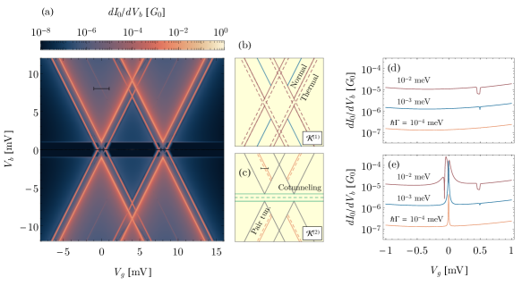
The numerical results for the differential conductance as a function of the gate and bias voltages are shown in Fig. 1 (a) for the representative parameters . In order to understand the features seen in this figure, we distinguish between normal and anomalous (Andreev) contributions to the dc current.
IV.1 Normal current
The normal current originates from the terms
| (49) | ||||
| (50) |
If we consider only these contributions, the only difference between a superconductor and a normal metal is the non-flat density of states. This is the so-called “semiconductor model” of the superconductor [78].
The normal terms produce a stability diagram which resembles the case of a SIAM coupled to normal electrodes, once the DOS is accounted for. In a similar way to the case of normal leads, one observes areas of reduced current due to the Coulomb interaction, the well-known Coulomb diamonds, and areas of current flow, which take the form of triangles, pointing at the charge degeneracy points . In addition, in the superconducting case, the gap opens a region of reduced current for
| (51) |
On top of that, additional resonant lines running parallel to the Coulomb diamonds and intersecting at can be observed. At these resonances, the current is carried by thermally excited quasiparticles above the gap, originating from the exponential tail of the Fermi function [79]. In Fig. 1 (b) we have represented schematically the main features appearing in the first order of perturbation theory, distinguishing normal contributions arising from quasiparticles below the gap (solid lines) and from the thermally excited quasiparticles (dashed lines). Moreover, we point out the presence of a faint feature exactly at the middle point between the normal and thermal lines, which is visible especially for voltages satisfying Eq. 51. This feature is the result of a non-zero subgap density of states due to the Dynes parameter. Then, exhibits a small step at due to the Fermi function and, as a result, one observes a faint conductance peak.
The main processes appearing at the second order are due to long-range virtual tunneling of quasiparticles across the dot, in the form of cotunneling, and pair tunneling. These features are represented schematically in Fig. 1 (c).
Cotunneling leads to the presence of a significant current in the Coulomb diamonds, larger than the contribution from the first order term. In the case of superconducting leads, cotunneling is suppressed for the range in Eq. 51 due to the unavailability of quasiparticle excitations inside the superconducting gap. As a result, the onset of cotunneling can be appreciated as a horizontal feature [86] (i.e. independent of the gate voltage ) in the differential conductance at , which can be seen clearly in Fig. 1 (a). It corresponds to the solid green lines in the scheme of Fig. 1 (c). Thermal effects also result in a finite current, albeit strongly reduced, extending to and producing a zero-bias conductance peak [86] [represented with a dashed red line in Fig. 1 (c)].
Quasiparticle pair tunneling involves the simultaneous transfer of two charges between the leads. Normal pair tunneling occurs prominently under the condition
| (52) |
which can be obtained by inspection of the integrals appearing in the pair tunneling kernel [86]. These resonances lines are displaced by a factor from the pair tunneling condition for normal leads, which corresponds to
| (53) |
However, thermal effects extend the area of effective pair tunneling from Eq. 52 to Eq. 53. This is indicated in the scheme of Fig. 1 (c) by orange lines (again, solid for the non-thermal and dashed for the thermal contributions).
The normal contribution to the dc current is represented for a small window around the pair tunneling resonance in Fig. 1 (d), for and different values of . This window is marked in Fig. 1 (a) by a black segment. We observe a conductance peak corresponding to normal pair tunneling at which becomes appreciable for and becomes more marked for . The thermal pair tunneling feature would appear as a peak or dip for the condition in Eq. 53 for larger tunneling rates and/or temperatures, but is too faint to be seen for the parameters considered here.
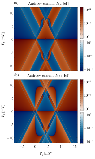
IV.2 Andreev current
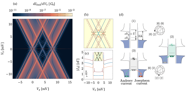
We consider now the Andreev current, corresponding to the anomalous contribution to the out of equilibrium dc current. It can be contrasted with the Josephson current, which is time-dependent for non-zero bias. In particular, the Andreev current occurs due to Cooper pair tunneling between a single superconducting lead and the quantum dot, whereas the Josephson current develops due to Cooper pair flow between two superconducting leads.
In the weak-coupling approximation, the Andreev current is given by
| (54) |
The first term originates from the first-order current kernel, and is of the form
| (55) |
If the lead indices in the arguments of the kernel and the coherence were not the same, this term would contribute to the Josephson current [see also Fig. 2 (d)]. Note that, despite involving a first order kernel, these terms are except at the pair tunneling resonances (this is discussed in more detail in Appendix C).
The second contribution originates from the second-order anomalous kernel, and reads
| (56) |
where the two anomalous arcs of belong to the same lead. These terms are always .
In Fig. 2 (a), we have represented the Andreev conductance for the same parameters as Fig. 1. Its main features have been schematized in Fig. 2 (b). Note that the color scale runs here from to , one order in higher than Fig. 1 (a). Overall, the Andreev current exhibits a similar profile as the full dc current, with “normal” features along the edges of the Coulomb diamonds, indicated by solid red lines in Fig. 2 (b). These lines originate from the coherence peaks of the anomalous DOS, due to the presence of a large number of energetically available quasiparticles near the gap [72]. Moreover, we find a peak in the conductance along the thermal lines [depicted with red dashed lines in the scheme of Fig. 2 (b)] for identical reasons.
The other prominent feature is a resonant behavior along the pair tunneling condition [namely Eq. 53, marked in blue in both Fig. 1 (b) and Fig. 2 (b)]. Under resonance, the Andreev current is instead of the usual , despite involving the exchange of two particles. This scaling is shown rigorously in Appendix C. However, anomalous pair tunneling is significantly reduced inside the Coulomb diamond, where the Cooper pair coherences are thermally suppressed. We have shown the Andreev current along one of the two resonances in Fig. 2 (c), exhibiting both the scaling and the suppression in the first Coulomb diamond. In Fig. 1 (e) we depicted the differential conductance calculated with all of the terms in the kernel, including the anomalous contributions for the same parameters as in Fig. 1 (d). We observe a strong feature precisely at the pair tunneling resonance at , as opposed to the resonance feature due to the normal processes, which is displaced by from the resonance condition, Eq. 53.
Moreover, in the current regions outside of the Coulomb diamonds, we find a remarkable feature: a bias-independent dip in the conductance (i.e. a vertical line) for gate voltages corresponding to the degeneracy points . This is the most distinct feature originating from , and reflects its vanishing along these lines. At , we can obtain an analytic expression for in the limit . Under this condition, the contributions to the Andreev current from both leads cancel each other due to symmetry and the equal populations of the empty and single occupied states. For , the same logic follows due to particle-hole symmetry of the stability diagram along the line . This is shown in more detail in Appendix G.
Finally, we have two weaker sets of peaks, corresponding to lower slope lines (compared to the Coulomb diamonds) and horizontal cotunneling-like lines. These are marked respectively by orange (solid or dashed for thermal contributions) and green lines in Fig. 2 (b). These features are visible in Fig. 2 (a) due to the lower range of the conductance, and correspond to effects which scale as or larger. The horizontal cotunneling-like lines (marked in green) are due to corrections to the density operator from the propagation kernel .
The lower slope lines, indicated in orange, are reminiscent of subgap features due to multiple Andreev reflections predicted in resonant tunneling junctions [87]. Here, however, due to the inclusion of Coulomb interactions, they occur within the Coulomb gap. While the slopes of the diamond amount to , the ones involving Cooper pair tunneling are given by . This reflects the energy needed to exchange a Cooper pair from one lead to the other. For the dc current, they appear as higher order corrections, which are not visible in the full result of Fig. 1, where cotunneling leads to an appreciable current inside the Coulomb diamond that masks these peaks. Processes involving the transfer of more Cooper pairs would yield even lower slopes: , but are not observed in the weak coupling limit.
We further discuss the two contributions to the Andreev current and separately in Appendix G. In particular, inside the Coulomb diamonds, the two contributions cancel each other as they come with similar magnitude but opposite sign.
V Josephson current
We move now to the time-dependent terms. Like we did with the Andreev current, we can differentiate contributions coming from the first order kernel, which have the form
| (57) |
with denoting the opposite lead to (for conciseness, here and onward we do not write explicitly the value of unless necessary). We denote the current originating from these terms as and , respectively for the critical and dissipative current. Note that, even if the current kernel is of first order, the contribution to the current will be of order outside of the pair-tunneling resonances.
Moreover, we have terms coming from the second order current kernel, of the form
| (58) |
We denote the resulting current terms by and for the critical and dissipative currents, respectively. The expressions for the kernels in second order are quite complex and we describe them in Appendix F. Other contributions exist, such as those coming from terms like . Since these are of higher order in , we do not discuss them here.
V.1 Critical current
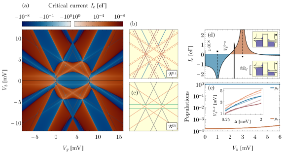
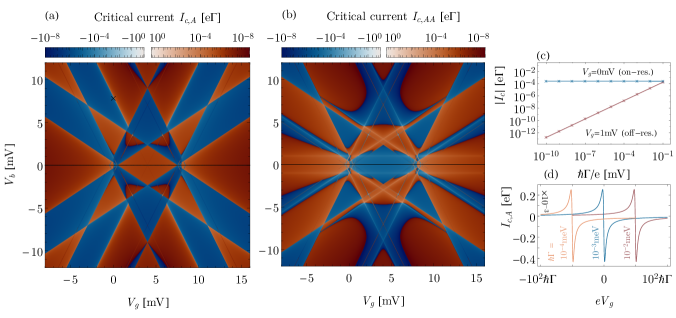
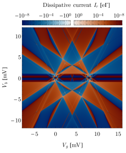
We have depicted the critical current as a function of the gate and bias voltages in Fig. 3 (a). We have represented its magnitude logarithmically as well as its sign by the color of the scale (red for positive and blue for negative sign). The features in the figure coming from the first order kernel are sketched in Fig. 3 (b), while the ones due to the second order kernel are shown in Fig. 3 (c). Moreover, the two contributions and are shown separately in Fig. 4 (a) and (b). We discuss now these features.
First, the Coulomb-diamond profile can be recognized in Fig. 3 (a). Along these lines, the proximity effect is amplified by the coherence peaks of the DOS, in a similar way to what occurs for the Andreev current. Likewise, we observe peaks in the Josephson current along the Cooper pair resonances [Eq. 53], marked in blue in Fig. 3 (b). These peaks are due to , and thus are observed in Fig. 4 (a). The proximity effect here is the largest as the unoccupied and doubly occupied states in the dot are resonant with the Cooper pairs of one of the leads, as mentioned above and discussed in detail in Appendix C. There, we show that the Josephson current along these resonances is instead of the usual . This is demonstrated numerically in Fig. 4 (c) and (d). In particular, (d) shows that the width of the resonance is also proportional to . Inside the central Coulomb diamond the Cooper pair resonances are thermally suppressed and the corresponding features are no longer seen.
The characteristic feature of the critical current is the presence of low slope lines, similar to the Andreev current. These are marked in orange in Fig. 3 (b) and (c). For the Andreev current these lines correspond to higher order processes and are barely noticeable in the full dc current of Fig. 1; however, for the critical current the low slope lines are a leading order feature. Inspecting the second order kernel , as given in Appendix F [i.e. Eq. 113], one observes a characteristic factor in the denominators, which results in a low slope. As mentioned in Section IV.2, this reflects the energy needed to exchange a Cooper pair from one lead to the other.
Finally, we observe gate-independent horizontal lines mirroring the cotunneling lines observed and discussed in the dc current. The origin of these lines is similarly the long-range transfer of charge from lead to lead with only virtual occupation of the dot. They appear only in , as can be seen in Fig. 4 (b).
The critical current exhibits a complex structure when it comes to the sign. For low bias voltages we can connect these findings to known results for the interacting SIAM at zero bias [39, 50]. We observe clearly a transition occurring near zero bias upon sweeping the gate voltage. It is signaled by a change of the sign of the supercurrent in the central Coulomb diamond compared to the neighboring diamonds with even occupancy. This change of sign remarkably extends to bias voltages . Here, it is useful to distinguish the behavior of from that of . For , the critical current is mostly positive in the central Coulomb diamond, near zero bias, except for two small pockets near the degeneracy points . Previous results in the low temperature limit indicate that the contribution from the first order kernel to the critical current is always positive [50]. However, thermal effects allow for a change of sign to occur even at this level of approximation due to quasiparticle-assisted processes. In contrast, is negative in the first Coulomb diamond for low bias, except near the resonances close to the degeneracy points.
Inside the central Coulomb diamond, we observe another change in sign in the full critical current as the voltage bias is increased. This sign change accompanies the low slope lines at first, close to the degeneracy points. As the bias voltage is increased further, the current goes back to negative for .
We have depicted the current for in Fig. 3 (d), as well as the populations of the odd and even sectors, namely
in Fig. 3 (e). Note, in particular, that the transition at , seen in Fig. 3 (c), is not accompanied with a change of the parity of the ground state. Instead, we can attribute this change to the competition between two processes: the feature occurring at (indicated with a square), with negative sign, and the one occurring at (marked with a dot), with positive sign. The former is the gate-independent cotunneling-like feature at , while the second originates from the low slope lines which meet in the center of the odd Coulomb diamond at . Here, the transition occurs precisely at the middle point between these two resonances. Following this logic, we can obtain a heuristic expression for the first transition at , which will occur for values of the bias voltage given by
| (59) |
We have calculated numerically for different values of and , shown in the inset of Fig. 3 (e). The heuristic curves of Eq. 59 have been represented with lighter colors. As can be seen there, they approximate qualitatively the true transition points.
Moreover, we have sketched the energetics corresponding to the two resonances in the insets of Fig. 3 (d), showcasing the distinct physics corresponding to the two resonances. The cotunneling-like feature occurs as the peaks of the two DOS functions align. Meanwhile, the low slope line corresponds to a Cooper pair-assisted process, where the peak of the electron (empty) part of the source DOS is separated by from the chemical potential of the dot at the 0-1 transition.
In a similar way, in the and charge Coulomb diamonds, the current around the low slope lines is of opposite sign to the rest of the diamond. Outside of the diamonds, undergoes a change of sign as the pair tunneling resonances are crossed, which is not present in (having no intrinsic pair tunneling features). This change in sign can be understood from the fact that the contribution to from lead is proportional to [see Eq. 84].
We note that, due to numerical errors, the resonance lines in the critical current usually exhibit small regions of the opposite sign, e.g. in correspondence with the normal slope thermal lines, visible in both Fig. 3 and Fig. 4. We associate these localized sign issues to convergence problems when dealing with the strongly peaked density of states. We refer to Appendix F for a more detailed discussion of the numerical implementation.
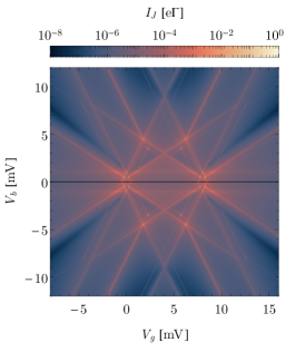
V.2 Dissipative contribution
The stability diagram of the dissipative contribution is presented in Fig. 5. We employ the same logarithmic scale as for , with the sign indicated by the color. The features of the dissipative current are similar to those of . Nonetheless, we outline some differences. First, we observe horizontal cotunneling-like features. Like for the dc current, and unlike for , we observe a stark reduction in the amplitude of the current for voltages . As for the critical and Andreev currents, we observe low slope lines, doubled as well into normal and thermal lines.
Regarding the sign of , we notice a similar change of sign in the central Coulomb diamond for . Crucially, the dissipative current is odd in the bias voltage, in a similar way to the dc current. Hence, it vanishes at zero bias, leaving only the sine term in Eq. 43. We observe sign changes occurring together with the presence of low slope lines. Here, unlike for , the sign change occurs along — instead of around — the resonance. Since is strongly suppressed for , we do not expect the sign changes in this region to be remarkable.
V.3 Josephson radiation
The time-dependent components of the current can be hard to detect in experimental circumstances. A viable way to do this is the measurement of the Josephson radiation [75, 70]. Hence, we close this section by considering the features that can be accessed via radiative measurements. In particular, we may consider an experimental setup similar to the one in [70]. There, a superconductor-insulator-superconductor (SIS) junction was employed as the detector, coupled to the S-QD-S junction via a waveguide resonator. The photo-assisted tunneling current through the SIS could be related to the amplitude of the Josephson current as , where
| (60) |
and is a voltage-dependent factor. It accounts for the current-voltage characteristic of the SIS junction and the impedance of the resonant circuit. We have shown as a function of the gate and voltage bias in Fig. 6. Most of the features present in the Josephson radiation have already been discussed in Sections V.1 and V.2. In particular, one sees both cotunneling-like features and low slope lines. The former are faint but observable in the results of [70].
VI Conclusion
In this work we have presented a full transport theory for quantum dot-based Josephson junctions. A particle-conserving theory of superconductivity in the particle number space was employed, which allows one to account for particle transfer in situations out of equilibrium. In this formulation, the Josephson effect arises naturally from the coherent dynamics of the Cooper pairs.
The theory is tailored to weakly coupled systems, whereby all processes up to second order in the hybridization strength were included. This encompasses sequential and virtual transfer of both quasiparticles and Cooper pairs. Specifically, we distinguished between the normal and the anomalous contributions to tunneling. The former conform to the usual “semiconductor model” of superconductivity [78]. The latter accounts for coherent Cooper pair transport and yields both an anomalous contribution to the dc current, the so-called Andreev current, as well as the Josephson current.
For the dc current, we have identified characteristic features at the Cooper pair-induced resonances, in which the quantum dot energetically favors the appearance of coherences involving both Cooper pairs and dot electrons. At these resonances, the current scales linearly with the tunneling rates, instead of the usual dependence on the square, and despite reflecting the transfer of two charges.
For the Josephson current, we obtained the full dependence of the critical current on the gate and on the bias voltage between the two superconducting leads. By studying its sign we have identified the extension of the well-known transition to out of equilibrium situations. We found, in particular, a rich behavior of the current (and its sign). While for the case of zero bias the change in sign can be related directly to the parity of the ground state, for non-zero bias these sign changes reflect a complex interplay of processes. For example, inside the Coulomb diamonds they arise from the competition between gate-independent Cooper pair cotunneling and gate dependent Cooper pair-assisted pair tunneling. We further present results for the dissipative current and the Josephson radiation, which exhibit similar features to the critical current.
The dc current has been measured in many different setups in the past, most notably in nanowire and carbon nanotube junctions [38]. Furthermore, measuring the Josephson radiation [75, 70] allows access to information about the time-dependent quantities. From the theoretical point of view, the formalism is extremely adaptative. While we considered the particularities of a single quantum dot junction, the model can be extended to arbitrary interacting nanojunctions directly.
Acknowledgements.
We thank Julian Siegl for discussion and help on this work, and Christoph Brückner for help with the numerical simulations. J.P.-C. and M.G. acknowledge DFG funding through Project B04 and A.D. through Project B02 of SFB 1277 Emerging Relativistic Phenomena in Condensed Matter. G. P. is supported by Spain’s MINECO through Grant No. PID2020-117787GB-I00 and by CSIC Research Platform PTI-001.Appendix A Stationary solutions of the GME
We sketch the derivation of the GME, Eq. 12, within the Nakajima-Zwanzig formalism [80, 81], focusing on the time-dependent solutions.
The full density operator, including quantum dot and leads, is a solution of the Liouville-von Neumann equation
| (61) |
The Nakajima-Zwanzig projector is now introduced
| (62) |
with an, in principle, arbitrary reference density operator . Provided that , we can write Eq. 61 as an equation only for as
| (63) | ||||
[compare Eq. 12] where we have defined
| (64) | ||||
| (65) |
We moreover assume that , allowing us to neglect the first term in the right-hand side of Eq. 63.
For the time-independent case considered here, we proceed by Laplace transforming Eq. 63, yielding
| (66) | ||||
with denoting Laplace transformation. The time-domain solution can be recovered through Mellin’s inverse formula
| (67) |
where is a real number such that all poles of lie to the left of the line in the complex plane. This integral can be calculated with the use of the residue theorem, employing a semicircular contour in the left complex half-plane. Then, provided that there are only first order poles in the contour, we recover directly the time evolution
| (68) |
where , defined in Eq. 15, are the residues at the poles . Upon taking the trace over the bath, we can define the kernel
| (69) |
which has the expanded form of Eq. 17. Then, Eq. 66 can be written as
| (70) |
The poles can be calculated by taking the limit in Eq. 70, yielding
| (71) |
The are the solutions to the non-linear eigenvalue equation
| (72) |
Here the determinant is understood to be of the linear application acting on the space of operators.
Appendix B GME for the quantum dot and Cooper pairs
We particularize the Nakajima-Zwanzig formalism to the case of a central system comprising both the quantum dot states and the Cooper pairs of the leads. The action of the current kernel can be written in the following manner, separating explicitly the action on the QD and CP sectors
| (74) |
where is , is defined in Eq. 28, and we introduce two difference vectors and which we consider as general for now.
Here, is a superoperator in the quantum dot space only. In order to arrive to an expression for it, we have to evaluate the effect of the kernel on the Cooper pair sector. This action comes in two forms. First, through the presence of the Cooper pair operators, and second through the action of , present in the free propagators [see Eq. 18], which needs to be resolved. In order to do so, we make use of , to move the Cooper pair operators to the left, as in Eq. 74. By this, we have included a shift in the argument of the kernel in Laplace space. This accounts for the action of when applied to a term such as the one appearing in Eq. 74. We could incorporate this as a shift in the Laplace variable because and always appear together in the propagators.
The current can be written in terms of the of Eq. 74 as
| (75) |
Since the kernel term is independent of the index , we can move the summation over to the density operator and introduce the simplified notation
| (76) |
with defined in Eq. 24 and
| (77) |
Note that we do not denote the in a particular manner, and distinguish them from the by the number of arguments. This shows that only the are needed in order to calculate the current. That is, we can freely sum over the and consider only the Cooper pair imbalance , with the information of the CP sector fully encoded into the . In this simplified notation, the term includes all kernel elements that change the number of Cooper pairs by , regardless of whether the Cooper pair operators act on the right or on the left. This can be seen from the fact that
We can perform a similar simplification of the GME. With Cooper pair numbers explicitly written, the equation for a term such as is given by
| (78) |
where again we have moved the Cooper pairs to the left and evaluated the in the same manner as for the current kernel. Then, we can sum over in Eq. 78. Defining
From this, the proof of Eq. 31 is direct. We can consider the NZE for a reduced quantum dot operator
This is the same equation as the one for , yielding the desired equivalence. Note that this must be satisfied for all , and hence the coefficients relating the two quantities, namely the , appearing in Eq. 31, must be independent of .
Within the mean field approximation of our model, these can be determined by considering the constant of motion
| (80) |
The fact that this quantity is conserved follows from the fact that the Cooper pair operators commute with the tunneling Hamiltonian. The time-dependent factor compensates for the time evolution of the Cooper pair operators due to the chemical potential of the leads. Since is purely a system operator, its expectation value can be evaluated from the reduced density operator, yielding at the initial time
This is to be compared with its value in a stationary state given by Eq. 32,
Since due to conservation of probability, together with Eq. 31, we see that is the only non-vanishing contribution. Then, employing this relation again
and comparing this with the initial value, it follows that
| (81) |
These coefficients can be related to the Fourier components of the function of [72]. Here, as mentioned in the main text, we assume that Eq. 27 has a single solution for . Otherwise, the different solutions to the GME may not be proportional.
Let us consider several instances of initial correlations and their corresponding . First, let us take an initial condition with no superconducting correlations, so that
| (82) |
It follows that . Taking into account Eq. 36, we find as a result and no Josephson effect will develop in the system.
Next, we consider an initial state of the form
| (83) | ||||
for some . This would correspond to a separable initial state with particle conservation enforced. The phase difference could develop, for instance, from relaxation processes unaccounted by the present model, which would relax the phase to the minimum of the Josephson potential [78] (Here is the conjugate operator to ). Then, Eq. 83 yields Eq. 37. This is the case considered in the main text.
Appendix C Analysis of the Cooper pair space structure
A complication with calculating the current within the theory outlined above is that the density operator is infinitely sized, as it incorporates coherences with infinitely many Cooper pair numbers. However, not all of these elements contribute in the same manner to the current. Coherences involving large imbalances in the Cooper pair numbers between the two leads can only be produced by high order tunneling events. Hence, in the weak coupling approximation employed here we expect that they will be negligible. As such, we have not only to consider which kernel elements are relevant (as was done above) but also which density operator coherences are. In this appendix, we develop the recipe for determining which coherences are relevant at a given perturbation level.
C.1 Relevant contributions to the density operator
Let us consider first . Probability conservation requires that , therefore the leading term in will be of order .
On the other hand, for a term with , there is no equivalent trace condition. Eq. 16 gives
| (84) |
Hence, in order to obtain the leading order contribution to them we need to inspect Eq. 84 and analyze the relevant kernels at each order.
We consider at first only the sequential tunneling approximation and disregard the denominator in Eq. 84. We know that is of order 1. Hence, terms such as will be of order , since is of order . This term appears in the sum for , which will then be of order itself. Higher coherences are not directly connected to For instance, is connected via to , and this is connected to via . Hence, will be at least of order . This indicates that the harmonics in the density operator can be ordered in a hierarchy, in which terms which are directly connected to will be of order , and any successive step away will be one order higher in .
This picture changes significantly when the denominator is taken into account. The same hierarchy holds in general, but whenever a matrix element satisfies
| (85) |
the denominator is of order itself and this component and all of the following components connected to it “skip” an order in this hierarchy. We say then that the coherence is resonant. E.g. the are of order 1 at the resonances of Eq. 53.
For the sequential tunneling approximation, provided that the condition Eq. 85 is satisfied by at most one value of (that is, there is no overlap between two or more resonances) only are relevant for the calculation of the density operator. Moreover, is only significant wherever the are resonant.
Regarding the second order, the main change in the structure of the kernel is that now there are also kernel components of the form , , and terms such as are now directly coupled to . However, they do so through a kernel component of order and the hierarchy still holds. The diagrams involving one normal and one anomalous arc are similar to the in sequential tunneling but are one order higher in . As a result, they are only relevant at resonances such as Eq. 53 where they give contributions of order to the density operator.
Hence, at second order it suffices to consider terms up to to obtain the density operator at order , provided again that there are no overlapping resonances. Moreover, the are only significant at the pair tunneling resonances.
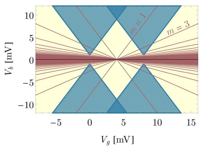
Continuing the logic for higher orders, we can classify the possible resonances into the two types discussed under Eq. 26. First, for , with , resonances occur at
| (86) |
These are resonant along lines with progressively lower slopes in the stability diagram, until eventually accumulating near for large . This is shown in Fig. 7.
Second, for , all of the coherences are resonant only for , regardless of . As such, considering only the coherences up to a certain in the density operator is justified when sufficiently far () from zero bias. A resummation can nonetheless be carried out for exactly [50]. The collapse of the hierarchy at zero bias reflects the degeneracy of the different Cooper pair number states in that case, since there is no energy transfer from one lead to the other when a Cooper pair is exchanged.
From this, we see that the overlap of resonances in the weak coupling limit occurs only close to .
C.2 Relevant contributions to the current
We turn now to the current. Therefore, we apply the current kernel superoperator to the density operator and inspect the scaling with .
For the sequential tunneling approximation, if no resonances are present, the main contribution to the dc current will come from , which is of order ; terms such as are of order in general. At the pair-tunneling resonances, however, the are of order because the are of order 1. For the Josephson current we find a similar situation. The only contribution from the first order kernel is . This is of order in general, but of order at the CP resonances.
The second order kernel does not change significantly these estimates. The main contributions to the Josephson current from the second order kernel are of order and arise from terms such as . The terms originating from kernels with one anomalous and one normal arc, such as , only contribute significantly at the pair tunneling resonances, where is of order 1 and hence they give contributions to the current of order . Crucially, these are of order elsewhere. Hence, proceeding in this manner allows one to single out all contributions to the current that are at least of order or , but also contributions which are of higher order are included. Another example would be , which adds to the Josephson current but is for . Alternatively, the secular approximation [88] can be employed, in which only terms of order and are strictly included; we do not consider it in this work.
Appendix D Diagrammatic rules in Liouville space
We summarize the rules needed to translate a given diagram to the expression .
-
1.
Draw vertices on a propagation line. Associate to the th vertex a Liouville index . In the following, is the rightmost vertex and is the leftmost.
-
2.
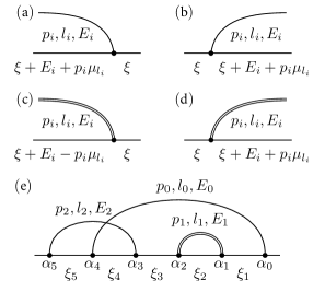
Draw all possible diagrams where each vertex is linked via a quasiparticle arc to another vertex. Discard diagrams which can be cut in two independent diagrams by removing the segment of the propagation line between two vertices without cutting a quasiparticle arc. The ith quasiparticle arc () is assigned an energy , a lead index , a Fock index , a spin and an index which can be either normal (represented by a single arc) or anomalous (double arc).
-
3.
Starting from the rightmost vertex and following the propagation line until the leftmost vertex:
-
(a)
For the th vertex, if it is the left vertex of the th quasiparticle arc, multiply by ; if it is the right vertex of a normal arc, multiply by ; if it is the right vertex of an anomalous arc, multiply by .
-
(b)
For the th segment of the propagation line between two vertices (), multiply by the propagator
The of the segment can be determined by conservation of energy in each vertex. Given two segments separated by the right vertex of a quasiparticle arc, the energy of the segment to the left must be larger by , where for a normal (anomalous) arc. Given two segments separated by the left vertex of an arc, the energy of the segment to the right must be larger by . This is shown in Fig. 8 .
-
(a)
-
4.
For each quasiparticle arc, multiply by , with the index of its rightmost vertex. If the arc is normal, multiply by ; if it is anomalous, multiply by . Multiply by for each crossing of two quasiparticle arcs.
-
5.
Sum over the internal (spin) and superoperator indices and integrate over the energies and multiply by . I.e.
For each combination of , the corresponding diagram is assigned to the kernel .
-
6.
To obtain the contribution to the current kernel, multiply by , where is the leftmost quasiparticle arc and .
Item 6 follows from the expression of the symmetrized current operator and the tunneling Liouvillian
| (87) | ||||
| (88) |
where and .
As an example, let us give the expression for the 3rd order diagram represented in Fig. 8 . We first obtain the lead energies in each segment of the propagator line, labeled in the diagram. Using Item 3b we obtain
| (89) | ||||
| (90) | ||||
| (91) | ||||
| (92) | ||||
| (93) |
This yields the following contribution
From Item 2 we see that this belongs to . The corresponding diagram for the current kernel can be obtained by taking and multiplying by within the summations.
Appendix E First order integrals
The sequential tunneling integral is given by Eq. 44. It can be calculated employing the residue theorem
| (94) |
Here, a Lorentzian cutoff has been introduced to regularize the integral for large . We introduce also the function
| (95) |
such that . We define the analytic continuation of having a branch cut at . In order to calculate , we define the contour (sketched in Fig. 9) as a semicircle extending in the upper (lower) half-plane with radius and separated by a distance from the real axis. In this manner, we have
| (96) |
The integrals over can be calculated employing the residue theorem. The Fermi function has poles at with residue , where , are the Matsubara frequencies. The Lorentzian has poles at with residue . Taking the limits, the integral yields
| (97) | ||||
| (98) | ||||
| (99) |
The infinitesimal factor reflects that the function is evaluated below the branch cut. This turns out to be only relevant in the calculation of the imaginary part of . The integral satisfies the property , which guarantees the hermiticity of the density operator.
The real valued function is mostly flat except for the region , where it exhibits a dip. For , the sampling at the Matsubara frequencies ignores the dip and the density of states is effectively flat. In that case, we recover the formula for normal leads [89]
| (100) | |||
| (101) | |||
where . Note that the encapsulates the logarithmic divergence in the limit .
In the opposite (low temperature) limit, , the sampling of by the Matsubara energies is taken as such small intervals that the sum over can be converted to an integral, with the differential defined as . This limit can be performed most conveniently by taking a hard cutoff instead of the Lorentzian in Eq. 94. Then, employing again the residue theorem and converting the resulting sums to integrals, one obtains
| (102) |

The equivalent of Eq. 94 for the anomalous kernel is given by
| (103) |
Contrary to the normal case, no Lorentzian regularization is needed, since the anomalous DOS decays as for large .
Before proceeding to contour integration, a question arises as to the analytic extension of the sgn function. Let us first define the function
| (104) |
If we choose the branch cut in its analytic continuation to lie in , has an extra branch cut on the imaginary axis. Fortunately, the branches can be chosen to remove this spurious branch cut. This is equivalent to considering the analytic continuation of as , which is the natural choice to take. With this, we can proceed as above to find
| (105) | ||||
| (106) |
Note that the function is real, since is purely imaginary. The anomalous second order integral satisfies . Since for , the Matsubara sum vanishes in the limit . In the opposite limit , we can transform again the sum into an integral and solve it analytically, yielding
| (107) |
Appendix F Second order kernel and integrals
We discuss in detail the second order kernels and discuss the numerical implementation employed to obtain the current and the density operator. We use the notation , with denoting the class of the diagram. Let us consider first the fully normal kernel (). After summing over the lead and Fock indices of the two lines, the D contribution is given by
| (108) |
Meanwhile, the fully normal X kernel is given by
| (109) |
For the mixed and anomalous contributions, it suffices to apply the following rules for each normal line that is turned from normal into anomalous, as per the diagrammatic rules. First, the following substitutions are performed:
| (110) | ||||
| (111) |
where the first refers to the rightmost vertex of the quasiparticle line. Then, for each propagator to the left of this vertex, we have to further substitute:
| (112) |
in order to account for Item 3b of the diagrammatic rules. Finally, the term now contributes to the kernel . For instance, let us turn the two lines of Eq. 108 from normal to anomalous yields. Now, the terms corresponding for the different values of will now contribute to distinct kernel components. Using the rules, we find
| (113) |
Here we have already taken into account that the only terms that are not zero for the QD Josephson junction have . The corresponding current kernels are obtained by taking and multiplying by .
The integrals that need to be calculated for these kernels have the form
| (114) | ||||
| (115) | ||||
where
| (116) |
Employing partial fraction decomposition, these integrals can be written as
| (117) | ||||
| (118) |
where we have defined the function
| (119) |
on which we will focus. In the limits and , the integrals of Eqs. 117 and 118 are equal to and , respectively.
In order to obtain the results presented in this work, we calculated the integral numerically on a grid and then obtained the derivative through finite differences. Small numerical errors appears when sampling the coherence peaks of the density of states. To help with convergence of the integrals, we consider in the grids, and set the Dynes parameter accordingly.
Lastly, employing the symmetry properties of this function, in particular
| (120) |
with the shorthand notation , it is possible to reduce the number of calculated grids by half. Even then, eight grids need to be calculated in the case of identical gaps for both leads, and four times that number for different gaps. Fortunately, Eq. 119 can be reduced to one-dimensional integrals by solving for the variable using the expression for the sequential tunneling integral given above.
Appendix G Contributions to the Andreev current
We discuss separately the two contributions to the Andreev current, and , which are represented in Fig. 10. We first point out that the two terms cancel inside the Coulomb diamonds almost exactly. This signals that the Andreev current is, outside of the resonances, intrinsically a second order process and that these two contributions must be understood together. We say here “almost exactly” because higher order contributions such as those discussed in Section IV.2 result in small differences. This can be appreciated here for the pair tunneling resonances close to , where shows a change in the current that is not observed in .
For we observe that the current changes sign close to but not exactly at the resonances, where the current is actually finite, as can be seen in Fig. 2 (c). For , we see the vertical features for , which appeared as dips in the differential conductance in Fig. 2. For we can study this feature employing an infinite interaction approximation to the Andreev current. Provided that , we find
| (121) | ||||
where is the population of the unoccupied state and with . Along the vertical line in the stability diagram due to symmetry, and we find
Since is odd in , [see Eq. 106], for equal tunneling rates and absolute values of the gap , the sum over the two leads cancels and the Andreev current is zero. This can be seen clearly in Fig. 10 (b) for . For , the analysis is the same due to particle-hole symmetry around .
We also remark the absence of features along the pair tunneling resonances for , which as pointed out above originate exclusively from .
References
- Cuevas et al. [1996] J. C. Cuevas, A. Martín-Rodero, and A. L. Yeyati, Phys. Rev. B 54, 7366 (1996).
- Cuevas et al. [2002] J. C. Cuevas, J. Heurich, A. Martín-Rodero, A. Levy Yeyati, and G. Schön, Phys. Rev. Lett. 88, 157001 (2002).
- Golubov et al. [2004] A. A. Golubov, M. Y. Kupriyanov, and E. Il’ichev, Rev. Mod. Phys. 76, 411 (2004).
- Bretheau et al. [2013] L. Bretheau, C. O. Girit, C. Urbina, D. Esteve, and H. Pothier, Phys. Rev. X 3, 041034 (2013).
- Oreg et al. [2010] Y. Oreg, G. Refael, and F. von Oppen, Phys. Rev. Lett. 105, 10.1103/physrevlett.105.177002 (2010).
- Cook and Franz [2011] A. Cook and M. Franz, Phys. Rev. B 84, 201105 (2011).
- Stanescu and Tewari [2013] T. D. Stanescu and S. Tewari, Journal of Physics: Condensed Matter 25, 233201 (2013).
- Tokura and Nagaosa [2018] Y. Tokura and N. Nagaosa, Nature Communications 9, 10.1038/s41467-018-05759-4 (2018).
- Baumgartner et al. [2021] C. Baumgartner, L. Fuchs, A. Costa, S. Reinhardt, S. Gronin, G. C. Gardner, T. Lindemann, M. J. Manfra, P. E. F. Junior, D. Kochan, J. Fabian, N. Paradiso, and C. Strunk, Nature Nanotechnology 17, 39 (2021).
- Baumgartner et al. [2022] C. Baumgartner, L. Fuchs, A. Costa, J. Picó-Cortés, S. Reinhardt, S. Gronin, G. C. Gardner, T. Lindemann, M. J. Manfra, P. E. F. Junior, D. Kochan, J. Fabian, N. Paradiso, and C. Strunk, Journal of Physics: Condensed Matter 34, 154005 (2022).
- Pfeffer et al. [2014] A. H. Pfeffer, J. E. Duvauchelle, H. Courtois, R. Mélin, D. Feinberg, and F. Lefloch, Phys. Rev. B 90, 075401 (2014).
- Meyer and Houzet [2017] J. S. Meyer and M. Houzet, Phys. Rev. Lett. 119, 136807 (2017).
- Doh et al. [2005] Y.-J. Doh, J. A. van Dam, A. L. Roest, E. P. A. M. Bakkers, L. P. Kouwenhoven, and S. D. Franceschi, Science 309, 272 (2005).
- Cleuziou et al. [2006] J.-P. Cleuziou, W. Wernsdorfer, V. Bouchiat, T. Ondarçuhu, and M. Monthioux, Nature Nanotechnology 1, 53 (2006).
- Pillet et al. [2010] J.-D. Pillet, C. H. L. Quay, P. Morfin, C. Bena, A. L. Yeyati, and P. Joyez, Nature Physics 6, 965 (2010).
- Dirks et al. [2011] T. Dirks, T. L. Hughes, S. Lal, B. Uchoa, Y.-F. Chen, C. Chialvo, P. M. Goldbart, and N. Mason, Nature Physics 7, 386 (2011).
- Delagrange et al. [2015] R. Delagrange, D. J. Luitz, R. Weil, A. Kasumov, V. Meden, H. Bouchiat, and R. Deblock, Phys. Rev. B 91, 241401 (2015).
- Siano and Egger [2004] F. Siano and R. Egger, Phys. Rev. Lett. 93, 047002 (2004).
- Sellier et al. [2005] G. Sellier, T. Kopp, J. Kroha, and Y. S. Barash, Phys. Rev. B 72, 174502 (2005).
- Karrasch et al. [2008] C. Karrasch, A. Oguri, and V. Meden, Phys. Rev. B 77, 024517 (2008).
- Chtchelkatchev and Nazarov [2003] N. M. Chtchelkatchev and Y. V. Nazarov, Phys. Rev. Lett. 90, 226806 (2003).
- Hays et al. [2021] M. Hays, V. Fatemi, D. Bouman, J. Cerrillo, S. Diamond, K. Serniak, T. Connolly, P. Krogstrup, J. Nygard, A. Levy Yeyati, A. Geresdi, and M. H. Devoret, Science 373, 430-433 (2021).
- Martín-Rodero and Yeyati [2011] A. Martín-Rodero and A. L. Yeyati, Advances in Physics 60, 899 (2011).
- Meden [2019] V. Meden, Journal of Physics: Condensed Matter 31, 163001 (2019).
- van Dam et al. [2006] J. A. van Dam, Y. V. Nazarov, E. P. A. M. Bakkers, S. D. Franceschi, and L. P. Kouwenhoven, Nature 442, 667 (2006).
- Jørgensen et al. [2007] H. I. Jørgensen, T. Novotný, K. Grove-Rasmussen, K. Flensberg, and P. E. Lindelof, Nano Letters 7, 2441 (2007).
- Maurand et al. [2012] R. Maurand, T. Meng, E. Bonet, S. Florens, L. Marty, and W. Wernsdorfer, Phys. Rev. X 2, 011009 (2012).
- Delagrange et al. [2016] R. Delagrange, R. Weil, A. Kasumov, M. Ferrier, H. Bouchiat, and R. Deblock, Phys. Rev. B 93, 195437 (2016).
- Li et al. [2017] X. Li, E. Barnes, J. P. Kestner, and S. Das Sarma, Phys. Rev. A 96, 012309 (2017).
- Eichler et al. [2009] A. Eichler, R. Deblock, M. Weiss, C. Karrasch, V. Meden, C. Schönenberger, and H. Bouchiat, Phys. Rev. B 79, 161407 (2009).
- Deacon et al. [2010] R. S. Deacon, Y. Tanaka, A. Oiwa, R. Sakano, K. Yoshida, K. Shibata, K. Hirakawa, and S. Tarucha, Phys. Rev. Lett. 104, 076805 (2010).
- Pillet et al. [2013] J.-D. Pillet, P. Joyez, R. Žitko, and M. F. Goffman, Phys. Rev. B 88, 045101 (2013).
- Bargerbos et al. [2022] A. Bargerbos, M. Pita-Vidal, R. Žitko, J. Ávila, L. J. Splitthoff, L. Grünhaupt, J. J. Wesdorp, C. K. Andersen, Y. Liu, L. P. Kouwenhoven, R. Aguado, A. Kou, and B. van Heck, PRX Quantum 3, 030311 (2022).
- Rozhkov and Arovas [1999] A. V. Rozhkov and D. P. Arovas, Phys. Rev. Lett. 82, 2788 (1999).
- Martín-Rodero and Yeyati [2012] A. Martín-Rodero and A. L. Yeyati, Journal of Physics: Condensed Matter 24, 385303 (2012).
- Clerk and Ambegaokar [2000] A. A. Clerk and V. Ambegaokar, Phys. Rev. B 61, 9109 (2000).
- Vecino et al. [2003] E. Vecino, A. Martín-Rodero, and A. L. Yeyati, Phys. Rev. B 68, 035105 (2003).
- Franceschi et al. [2010] S. D. Franceschi, L. Kouwenhoven, C. Schönenberger, and W. Wernsdorfer, Nature Nanotechnology 5, 703 (2010).
- Glazman and Matveev [1989] L. I. Glazman and K. A. Matveev, Soviet Journal of Experimental and Theoretical Physics Letters 49, 659 (1989).
- Choi et al. [2000] M.-S. Choi, C. Bruder, and D. Loss, Phys. Rev. B 62, 13569 (2000).
- Novotný et al. [2005] T. Novotný, A. Rossini, and K. Flensberg, Phys. Rev. B 72, 224502 (2005).
- Schoeller and Schön [1994] H. Schoeller and G. Schön, Phys. Rev. B 50, 18436 (1994).
- König et al. [1996a] J. König, H. Schoeller, and G. Schön, Phys. Rev. Lett. 76, 1715 (1996a).
- König et al. [1996b] J. König, J. Schmid, H. Schoeller, and G. Schön, Phys. Rev. B 54, 16820 (1996b).
- Kern and Grifoni [2013] J. Kern and M. Grifoni, The European Physical Journal B 86, 10.1140/epjb/e2013-40618-9 (2013).
- Magazzù and Grifoni [2022] L. Magazzù and M. Grifoni, Phys. Rev. B 105, 125417 (2022).
- Donarini and Grifoni [2024] A. Donarini and M. Grifoni, Quantum Transport in Interacting Nanojunctions (Springer, 2024).
- Saptsov and Wegewijs [2012] R. B. Saptsov and M. R. Wegewijs, Phys. Rev. B 86, 235432 (2012).
- Pala et al. [2007] M. G. Pala, M. Governale, and J. König, New Journal of Physics 9, 278 (2007).
- Governale et al. [2008] M. Governale, M. G. Pala, and J. König, Physical Review B 77, 10.1103/physrevb.77.134513 (2008).
- Moghaddam et al. [2012] A. G. Moghaddam, M. Governale, and J. König, Phys. Rev. B 85, 094518 (2012).
- Recher et al. [2001] P. Recher, E. V. Sukhorukov, and D. Loss, Phys. Rev. B 63, 165314 (2001).
- Probst et al. [2016] B. Probst, F. Domínguez, A. Schroer, A. L. Yeyati, and P. Recher, Phys. Rev. B 94, 155445 (2016).
- Hussein et al. [2016] R. Hussein, L. Jaurigue, M. Governale, and A. Braggio, Phys. Rev. B 94, 235134 (2016).
- Hussein et al. [2019] R. Hussein, M. Governale, S. Kohler, W. Belzig, F. Giazotto, and A. Braggio, Phys. Rev. B 99, 075429 (2019).
- Kumar et al. [2014] A. Kumar, M. Gaim, D. Steininger, A. L. Yeyati, A. Martín-Rodero, A. K. Hüttel, and C. Strunk, Phys. Rev. B 89, 075428 (2014).
- Kiršanskas et al. [2015] G. Kiršanskas, M. Goldstein, K. Flensberg, L. I. Glazman, and J. Paaske, Phys. Rev. B 92, 235422 (2015).
- Eldridge et al. [2010] J. Eldridge, M. G. Pala, M. Governale, and J. König, Phys. Rev. B 82, 184507 (2010).
- Sothmann et al. [2014] B. Sothmann, S. Weiss, M. Governale, and J. König, Phys. Rev. B 90, 220501 (2014).
- Sothmann and Tiwari [2015] B. Sothmann and R. P. Tiwari, Phys. Rev. B 92, 014504 (2015).
- Futterer et al. [2013] D. Futterer, J. Swiebodzinski, M. Governale, and J. König, Phys. Rev. B 87, 014509 (2013).
- Ortmanns et al. [2023a] L. C. Ortmanns, M. R. Wegewijs, and J. Splettstoesser, SciPost Physics 14, 10.21468/scipostphys.14.5.095 (2023a).
- Ortmanns et al. [2023b] L. C. Ortmanns, J. Splettstoesser, and M. R. Wegewijs, Phys. Rev. B 108, 085426 (2023b).
- Dell’Anna et al. [2008] L. Dell’Anna, A. Zazunov, and R. Egger, Phys. Rev. B 77, 104525 (2008).
- Jonckheere et al. [2009] T. Jonckheere, A. Zazunov, K. V. Bayandin, V. Shumeiko, and T. Martin, Phys. Rev. B 80, 184510 (2009).
- Andersen et al. [2011] B. M. Andersen, K. Flensberg, V. Koerting, and J. Paaske, Phys. Rev. Lett. 107, 256802 (2011).
- Hiltscher et al. [2012] B. Hiltscher, M. Governale, and J. König, Phys. Rev. B 86, 235427 (2012).
- Rentrop et al. [2014] J. F. Rentrop, S. G. Jakobs, and V. Meden, Phys. Rev. B 89, 235110 (2014).
- Lamic et al. [2020] B. Lamic, J. S. Meyer, and M. Houzet, Phys. Rev. Res. 2, 033158 (2020).
- Watfa et al. [2021] D. Watfa, R. Delagrange, A. Kadlecová, M. Ferrier, A. Kasumov, H. Bouchiat, and R. Deblock, Phys. Rev. Lett. 126, 126801 (2021).
- Josephson [1962] B. D. Josephson, Physics Letters 1, 251 (1962).
- Siegl et al. [2023] J. Siegl, J. Picó-Cortés, and M. Grifoni, Phys. Rev. B 107, 115405 (2023).
- Harris [1974] R. E. Harris, Phys. Rev. B 10, 84 (1974).
- Waldram [1976] J. R. Waldram, Reports on Progress in Physics 39, 751 (1976).
- Deacon et al. [2017] R. S. Deacon, J. Wiedenmann, E. Bocquillon, F. Domínguez, T. M. Klapwijk, P. Leubner, C. Brüne, E. M. Hankiewicz, S. Tarucha, K. Ishibashi, H. Buhmann, and L. W. Molenkamp, Phys. Rev. X 7, 021011 (2017).
- Leggett [2006] A. J. Leggett, Quantum Liquids: Bose Condensation and Cooper Pairing in Condensed-Matter Systems (Oxford Graduate Texts) (Oxford University Press, 2006).
- Picó-Cortés [2021] J. Picó-Cortés, AC dynamics of quantum dots and Josephson junctions for quantum technologies, Ph.D. thesis, Universidad Autónoma de Madrid (2021).
- Tinkham [2004] M. Tinkham, Introduction to Superconductivity: Second Edition (Dover Books on Physics) (Dover Publications, 2004).
- Pfaller et al. [2013] S. Pfaller, A. Donarini, and M. Grifoni, Phys. Rev. B 87, 155439 (2013).
- Nakajima [1958] S. Nakajima, Progress of Theoretical Physics 20, 948 (1958).
- Zwanzig [1960] R. Zwanzig, The Journal of Chemical Physics 33, 1338 (1960).
- Note [1] Nonetheless, we note that the GME is a full reformulation of the problem and the effect of the leads is considered exactly.
- Bruder and Schoeller [1994] C. Bruder and H. Schoeller, Phys. Rev. Lett. 72, 1076 (1994).
- Josephson [1964] B. D. Josephson, Rev. Mod. Phys. 36, 216 (1964).
- Josephson [1965] B. D. Josephson, Advances in Physics 14, 419 (1965).
- Ratz et al. [2014] S. Ratz, A. Donarini, D. Steininger, T. Geiger, A. Kumar, A. K. Hüttel, C. Strunk, and M. Grifoni, New Journal of Physics 16, 123040 (2014).
- Johansson et al. [1999] G. Johansson, E. N. Bratus, V. S. Shumeiko, and G. Wendin, Phys. Rev. B 60, 1382 (1999).
- Koller et al. [2010] S. Koller, M. Grifoni, M. Leijnse, and M. R. Wegewijs, Phys. Rev. B 82, 235307 (2010).
- Koller [2010] S. Koller, Spin phenomena and higher order effects in transport across interacting quantum-dots (2010), please check the errata to this publication (see URL for "Supplementary Material").