Matrix norm shrinkage estimators and priors

Abstract

We develop a class of minimax estimators for a normal mean matrix under the Frobenius loss, which generalizes the James–Stein and Efron–Morris estimators. It shrinks the Schatten norm towards zero and works well for low-rank matrices. We also propose a class of superharmonic priors based on the Schatten norm, which generalizes Stein’s prior and the singular value shrinkage prior. The generalized Bayes estimators and Bayesian predictive densities with respect to these priors are minimax. We examine the performance of the proposed estimators and priors in simulation.

1 Introduction

Suppose that we have a matrix observation $X\in\mathbb{R}^{n\times m}$ whose entries are independent normal random variables $X_{ij}\sim{\rm N}(M_{ij},1)$, where $n\geq m$ and $M\in\mathbb{R}^{n\times m}$ is an unknown mean matrix. In this setting, we consider estimation of $M$ under the Frobenius loss

$$l(M,\hat{M})=\|\hat{M}-M\|_{\mathrm{F}}^{2}=\sum_{i=1}^{n}\sum_{j=1}^{m}(\hat{M}_{ij}-M_{ij})^{2}.$$

Although the maximum likelihood estimator $\hat{M}=X$ is minimax, it is inadmissible when $nm\geq 3$ from Stein’s paradox (Stein, 1974).

There are two important minimax estimators that dominate the maximum likelihood estimator. One is the James–Stein (JS) estimator (James and Stein, 1961) given by

$$\hat{M}_{\mathrm{JS}}=\Big{(}1-\frac{nm-2}{\|X\|_{\mathrm{F}}^{2}}\Big{)}X.$$ (1.1)

This estimator shrinks towards the zero matrix. The other is the Efron–Morris (EM) estimator (Efron and Morris, 1972) given by

$$\hat{M}_{\mathrm{EM}}=X\left(I_{m}-(n-m-1)(X^{\top}X)^{-1}\right).$$ (1.2)

This estimator shrinks towards the space of low-rank matrices. Namely, let $X=USV^{\top}$, $U\in\mathbb{R}^{n\times m}$, $V\in\mathbb{R}^{m\times m}$, $S={\rm diag}(s_{1},\dots,s_{m})$ be the singular value decomposition of $X$, where $U^{\top}U=V^{\top}V=I_{m}$ and $s_{1}\geq\cdots\geq s_{m}\geq 0$ are the singular values of $X$. Then, $\hat{M}_{{\rm EM}}=U\hat{\Sigma}V^{\top}$ with $\hat{\Sigma}={\rm diag}(\hat{\sigma}_{1},\dots,\hat{\sigma}_{m})$, where

$$\hat{\sigma}_{i}=\left(1-\frac{n-m-1}{s_{i}^{2}}\right)s_{i},\quad i=1,\ldots,m.$$

Thus, the Efron–Morris estimator shrinks the singular values towards zero and works well when $M$ is close to low-rank (see Matsuda and Strawderman (2022) for details). Note that the number of nonzero singular values of a matrix is equal to its rank. Thus, the James–Stein and Efron–Morris estimators can be viewed as scalar and matricial shrinkage estimators, respectively. Recently, Yuasa and Kubokawa (2023) proposed a minimax estimator that combines these two estimators by using a weight determined by minimizing an unbiased estimate of risk.

Correspondingly, there are two important superharmonic priors of $M$, where a prior $\pi(M)$ is said to be superharmonic if

$$\Delta\pi(M)=\sum_{i=1}^{n}\sum_{j=1}^{m}\frac{\partial^{2}\pi}{\partial M_{ij}^{2}}(M)\leq 0$$

for every $M$. One is Stein’s prior (Stein, 1974) given by

$$\pi_{\mathrm{S}}(M)=\|M\|_{\mathrm{F}}^{2-nm},$$ (1.3)

for $nm\geq 3$. The generalized Bayes estimator with respect to Stein’s prior shrinks towards the origin like the James–Stein estimator (1.1). The other is the singular value shrinkage (SVS) prior (Matsuda and Komaki, 2015) given by

$$\pi_{\mathrm{SVS}}(M)=\det(M^{\top}M)^{-(n-m-1)/2},$$ (1.4)

for $n-m\geq 2$. The generalized Bayes estimator with respect to the singular value shrinkage prior shrinks the singular values towards zero like the Efron–Morris estimator (1.2). Since a generalized Bayes estimator with respect to a superharmonic prior is minimax (Stein, 1974), the generalized Bayes estimators with respect to these priors are minimax under the Frobenius loss. See Tsukuma (2008); Tsukuma and Kubokawa (2017) for other types of minimax (generalized) Bayes estimators. Similarly, the Bayesian predictive densities with respect to these superharmonic priors are minimax under the Kullback–Leibler loss (Komaki, 2001; George et al., 2006; Matsuda and Komaki, 2015).

In this study, we propose a broad class of shrinkage estimators and priors by generalizing the above ones. It is based on the (quasi-)norm of a matrix $A$ defined by

$$\|A\|_{p}=\Big{(}\sum_{i=1}^{m}\sigma_{i}^{p}\Big{)}^{1/p},$$ (1.5)

for $p>0$, where $\sigma_{1}\geq\cdots\geq\sigma_{m}$ are the singular values of $A$. For $p\geq 1$, it is called the Schatten norm. In particular, the Schatten norm with $p=2$ coincides with the Frobenius norm and the Schatten norm with $p=1$ is called the nuclear norm, which is often used for low-rank regularization. Note that $\|\cdot\|_{p}$ with $p\in(0,1)$ is not a norm but a quasinorm. We derive sufficient conditions for the proposed estimators to be minimax and for the proposed priors to be superharmonic. Numerical results show their advantages compared to existing ones.

This paper is organized as follows. In Section 2, we introduce a class of matrix norm shrinkage estimators. In Section 3, we propose a class of matrix norm shrinkage priors associated with the estimators in Section 2. Numerical experiments are presented in Section 4. Technical lemmas are given in the Appendix with proofs.

2 Matrix norm shrinkage estimator

Let $X=USV$ be a singular value decomposition of $X$, where ${S}=\mathrm{diag}(s_{1},\dots,s_{m})$ with $s_{1}\geq\dots\geq s_{m}\geq 0$. We consider an equivariant estimator

$$\hat{M}=U\hat{\Sigma}V,$$ (2.1)

where $\hat{\Sigma}=\mathrm{diag}(\hat{\sigma}_{1}(s),\dots,\hat{\sigma}_{m}(s))$ and $s=(s_{1},\dots,s_{m})$. For convenience, we specify such an equivariant estimator by using $\hat{\sigma}_{1},\dots,\hat{\sigma}_{m}$ in the following. An unbiased estimate of its Frobenius risk has been derived as follows, which also appeared in Tsukuma (2008); Candes et al. (2013).

Proposition 1.

(Stein, 1974; Matsuda and Strawderman, 2019) For an equivariant estimator $\hat{M}$ in (2.1) with $\hat{\sigma}_{i}=(1-\phi_{i}(s))s_{i}$ for $i=1,\dots,m$, its Frobenius risk is given by

$${\rm E}_{M}\left[\|\hat{M}-M\|_{\mathrm{F}}^{2}\right]={\rm E}_{M}\left[nm+\sum_{i=1}^{m}\Big{\{}s_{i}^{2}\phi_{i}^{2}-2(n-m+1)\phi_{i}-2s_{i}\frac{\partial\phi_{i}}{\partial s_{i}}\Big{\}}-4\sum_{i<j}\frac{s_{i}^{2}\phi_{i}-s_{j}^{2}\phi_{j}}{s_{i}^{2}-s_{j}^{2}}\right].$$

By extending the James–Stein and Efron–Morris estimators, we introduce the equivariant estimator $\hat{M}_{p,\alpha}$ defined by

$$\hat{\sigma}_{i}=\left(1-\alpha\frac{s_{i}^{p-2}}{\sum_{j=1}^{m}s_{j}^{p}}\right)s_{i},\quad i=1,\dots,m.$$

Note that the James–Stein estimator (1.1) corresponds to $p=2$ and $\alpha=nm-2$, whereas the Efron–Morris estimator (1.2) corresponds to $p=0$ and $\alpha=m(n-m-1)$. This estimator attains minimaxity for an appropriate choice of $p$ and $\alpha$ as follows.

Theorem 1.

For $p\in[1,2]$, $\hat{M}_{p,\alpha}$ is minimax if $\alpha\in[0,2nm-(2-p)m(m+1)-2p].$ For $p\in(0,1)$, $\hat{M}_{p,\alpha}$ is minimax if $\alpha\in[0,2nm-2m(m+1)+2(m-1)p].$

Proof.

Let $A=\sum_{i=1}^{m}s_{i}^{p}$, $B=\sum_{i=1}^{m}s_{i}^{p-2}$, and $C=\sum_{i=1}^{m}s_{i}^{2p-2}$. Substituting $\phi_{i}=\alpha s_{i}^{p-2}/(\sum_{j=1}^{m}s_{j}^{p})$ into the unbiased estimate of risk in Proposition 1 yields

$$nm+\sum_{i=1}^{m}\Big{\{}\frac{\alpha^{2}s_{i}^{2p-2}}{A^{2}}-\frac{2(n-m+1)\alpha s_{i}^{p-2}}{A}+\frac{2p\alpha s_{i}^{2p-2}}{A^{2}}-\frac{2(p-2)\alpha s_{i}^{p-2}}{A}\Big{\}}-4\alpha\sum_{i<j}\frac{s_{i}^{p}-s_{j}^{p}}{(s_{i}^{2}-s_{j}^{2})A}$$

$$=nm+\frac{\alpha}{A^{2}}\Big{\{}(\alpha+2p)C-2(n-m+p-1)AB-4A\sum_{i<j}\frac{s_{i}^{p}-s_{j}^{p}}{s_{i}^{2}-s_{j}^{2}}\Big{\}}.$$ (2.2)

Thus, if (2.2) is not larger than $nm$ for every $X$, the estimator $\hat{M}_{p,\alpha}$ is minimax.

First, assume $p\in[1,2]$. Since $AB\geq mC$ from Lemma 3 and

$$A\sum_{i<j}\frac{s_{i}^{p}-s_{j}^{p}}{s_{i}^{2}-s_{j}^{2}}\geq\frac{pm(m-1)}{4}C$$

from Lemma 5, the unbiased estimate of risk (2.2) is bounded from above by

$$nm+\frac{\alpha C}{A^{2}}\Big{\{}\alpha+2p-2(n-m+p-1)m-pm(m-1)\Big{\}},$$ (2.3)

which is not larger than $nm$ when $\alpha\leq 2nm-(2-p)m(m+1)-2p$.

Next, assume $p\in(0,1)$. From $A>0$ and $AB\geq mC$ from Lemma 3, the unbiased estimate of risk (2.2) is bounded from above by

$$nm+\frac{\alpha C}{A^{2}}\Big{\{}\alpha+2p-2(n-m+p-1)m\Big{\}},$$ (2.4)

which is not greater than $nm$ when $\alpha\leq 2nm-2m(m+1)+2(m-1)p.$ ∎

When $p\in[1,2]$, the upper bound (2.3) of the unbiased risk estimate (2.2) is minimized at $\alpha=nm-(1-p/2)m(m+1)-p.$ Thus, this value of $\alpha$ can be considered as a default choice. For $p=1$, it is given by $\alpha=nm-m(m+1)/2-1$.

We refer to $\hat{M}_{p,\alpha}$ with $p=1$ and $\alpha=nm-m(m+1)/2-1$ as the nuclear norm shrinkage (NNS) estimator and denote it by $\hat{M}_{\mathrm{NNS}}$. This estimator shrinks the singular values by a constant value that depends on the nuclear norm $\|X\|_{1}=\sum_{j=1}^{m}s_{j}$ of $X$:

$$\hat{\sigma}_{i}=s_{i}-\frac{nm-m(m+1)/2-1}{\sum_{j=1}^{m}s_{j}},\quad i=1,\dots,m.$$ (2.5)

From Corollary 3.1 of Tsukuma (2008), $\hat{M}_{\mathrm{NNS}}$ is dominated by its positive-part, which we call $\hat{M}_{\mathrm{NNS+}}$. Namely, $\hat{M}_{\mathrm{NNS+}}$ is defined by

$$\hat{\sigma}_{i}=\max\left(s_{i}-\frac{nm-m(m+1)/2-1}{\sum_{j=1}^{m}s_{j}},0\right),\quad i=1,\dots,m.$$

Remark 1.

Note that $\hat{M}_{\mathrm{NNS+}}$ has a similar form to the Singular Value Thresholding (SVT) estimator by Cai et al. (2010): $\hat{\sigma}_{i}=\max(s_{i}-\lambda,0)$, which is the solution of the nuclear norm regularized optimization problem: $\min_{M}\{-\log p(X\mid M)+\lambda\|M\|_{1}\}.$ This estimator is widely used in the estimation of low-rank matrices. In practice, the regularization parameter $\lambda$ is usually determined by minimizing Stein’s unbiased risk estimate (Candes et al., 2013). The estimator $\hat{M}_{\mathrm{NNS+}}$ can be viewed as determining $\lambda$ based on the nuclear norm of $X$: $\lambda=(nm-m(m+1)/2-1)/\|X\|_{1}$. While $\hat{M}_{\mathrm{NNS+}}$ may not work better than SVT in estimation of low-rank matrices, $\hat{M}_{\mathrm{NNS+}}$ attains minimaxity.

We also develop another class of minimax estimators. Let $\hat{M}^{*}_{p,\alpha}$ be an equivariant estimator defined by

$$\hat{\sigma}_{i}=s_{i}-\alpha s_{i}^{p-1},\quad i=1,\dots,m.$$

When $n-m+p-1>0$, the unbiased estimate of risk in Proposition 1 for $\hat{M}^{*}_{p,\alpha}$ is

$$nm+\alpha\left\{\alpha\sum_{i=1}^{m}s_{i}^{2p-2}-2(n-m+p-1)\sum_{i=1}^{m}s_{i}^{p-2}-4\sum_{i<j}\frac{s_{i}^{p}-s_{j}^{p}}{s_{i}^{2}-s_{j}^{2}}\right\},$$

which is minimized with respect to $\alpha$ at

$$\alpha(s,p)=\left(\sum_{i=1}^{m}s_{i}^{2p-2}\right)^{-1}\left((n-m+p-1)\sum_{i=1}^{m}s_{i}^{p-2}+2\sum_{i<j}\frac{s_{i}^{p}-s_{j}^{p}}{s_{i}^{2}-s_{j}^{2}}\right).$$ (2.6)

Thus, we consider the estimator $\hat{M}^{*}_{p}$ defined by

$$\hat{\sigma}_{i}=s_{i}-\alpha(s,p)s_{i}^{p-1},\quad i=1,\dots,m.$$

For $p=2$, it is approximately equal to the James–Stein estimator from $\alpha(s,2)=nm/(\sum_{i=1}^{m}s_{i}^{2})$. For $p=0$, it coincides with the Efron–Morris estimator from $\alpha(s,0)=n-m-1$. This estimator attains minimaxity under certain conditions as follows.

Theorem 2.

For $p\in(0,1]$, $\hat{M}^{*}_{p}$ is minimax if $n-m\geq 5-3p$.

Proof.

In general, the unbiased estimate of risk in Proposition 1 for the equivariant estimator

$$\hat{\sigma}_{i}=s_{i}-\alpha(s)s_{i}^{p-1},\quad i=1,\dots,m.$$

is

$$nm+\sum_{i=1}^{m}\Big{\{}s_{i}^{2p-2}\alpha(s)^{2}-2(n-m+p-1)s_{i}^{p-2}\alpha(s)-2s_{i}^{p-1}\frac{\partial\alpha(s)}{\partial s_{i}}\Big{\}}-4\sum_{i<j}\alpha(s)\frac{s_{i}^{p}-s_{j}^{p}}{s_{i}^{2}-s_{j}^{2}}.$$

By substituting (2.6), the unbiased estimate is equal to

$$nm+\alpha(s,p)\Big{\{}\alpha(s,p)\sum_{i=1}^{m}s_{i}^{2p-2}-2(n-m+p-1)\sum_{i=1}^{m}s_{i}^{p-2}-4\sum_{i<j}\frac{s_{i}^{p}-s_{j}^{p}}{s_{i}^{2}-s_{j}^{2}}\Big{\}}-2\sum_{i=1}^{m}s_{i}^{p-1}\frac{\partial\alpha(s,p)}{\partial s_{i}}$$

$$=nm-\Big{\{}(n-m+p-1)\sum_{i=1}^{m}s_{i}^{p-2}+2\sum_{i<j}\frac{s_{i}^{p}-s_{j}^{p}}{s_{i}^{2}-s_{j}^{2}}\Big{\}}^{2}/(\sum_{i=1}^{m}s_{i}^{2p-2})-2\sum_{i=1}^{m}s_{i}^{p-1}\frac{\partial\alpha(s,p)}{\partial s_{i}}.$$ (2.7)

From $p\leq 1,$

$$\sum_{i=1}^{m}s_{i}^{p-1}\frac{\partial\alpha(s,p)}{\partial s_{i}} \geq\sum_{i=1}^{m}s_{i}^{p-1}\frac{(n-m+p-1)(p-2)s_{i}^{p-3}+2\sum_{j\neq i}\frac{(p-2)s_{i}^{p+1}-ps_{i}^{p-1}s_{j}^{2}+2s_{i}s_{j}^{p}}{(s_{i}^{2}-s_{j}^{2})^{2}}}{\sum_{i=1}^{m}s_{i}^{2p-2}}$$

$$=\frac{(n-m+p-1)(p-2)\sum_{i=1}^{m}s_{i}^{2p-4}+2\sum_{i<j}\frac{(p-2)(s_{i}^{2p}+s_{j}^{2p})-ps_{i}^{2p-2}s_{j}^{2}-ps_{j}^{2p-2}s_{i}^{2}+4s_{i}^{p}s_{j}^{p}}{s_{i}^{4}+s_{j}^{4}-2s_{i}^{2}s_{j}^{2}}}{\sum_{i=1}^{m}s_{i}^{2p-2}}$$ (2.8)

Also, from $s_{i}^{2p}+s_{j}^{2p}\leq(s_{i}^{4}+s_{j}^{4})s_{i}^{p-2}s_{j}^{p-2}$ and $s_{i}^{2p-2}s_{j}^{2}+s_{i}^{2p-2}s_{i}^{2}\leq(s_{i}^{4}+s_{j}^{4})s_{i}^{p-2}s_{j}^{p-2}$,

$$\frac{(p-2)(s_{i}^{2p}+s_{j}^{2p})-ps_{i}^{2p-2}s_{j}^{2}-ps_{j}^{2p-2}s_{i}^{2}+4s_{i}^{p}s_{j}^{p}}{s_{i}^{4}+s_{j}^{4}-2s_{i}^{2}s_{j}^{2}}\geq-2s_{i}^{p-2}s_{j}^{p-2}.$$ (2.9)

Therefore, using (2.8), (2.9), and $(n-m+p-1)(p-2)\leq-2$,

$$\sum_{i=1}^{m}s_{i}^{p-1}\frac{\partial\alpha(s,p)}{\partial s_{i}} \geq\frac{(n-m+p-1)(p-2)\sum_{i=1}^{m}s_{i}^{2p-4}+2\sum_{i<j}(-2)s_{i}^{p-2}s_{j}^{p-2}}{\sum_{i=1}^{m}s_{i}^{2p-2}}$$

$$\geq(n-m+p-1)(p-2)(\sum_{i=1}^{m}s_{i}^{p-2})^{2}/(\sum_{i=1}^{m}s_{i}^{2p-2}).$$ (2.10)

From (2.10), the unbiased loss estimator (2.7) is bounded from above by

$$nm-\Big{\{}(n-m+p-1)\sum_{i=1}^{m}s_{i}^{p-2}\Big{\}}^{2}/(\sum_{i=1}^{m}s_{i}^{2p-2})-2\sum_{i=1}^{m}s_{i}^{p-1}\frac{\partial\alpha(s,p)}{\partial s_{i}}$$

$$\leq\ nm-\Big{\{}(n-m+p-1)\sum_{i=1}^{m}s_{i}^{p-2}\Big{\}}^{2}/(\sum_{i=1}^{m}s_{i}^{2p-2})-2(n-m+p-1)(p-2)(\sum_{i=1}^{m}s_{i}^{p-2})^{2}/(\sum_{i=1}^{m}s_{i}^{2p-2})$$

$$=\ nm-\big{[}(n-m+p-1)^{2}+2(n-m+p-1)(p-2)\big{]}(\sum_{i=1}^{m}s_{i}^{p-2})^{2}/(\sum_{i=1}^{m}s_{i}^{2p-2}).$$

It is smaller than $nm$ if $(n-m+p-1)^{2}+2(n-m+p-1)(p-2)\geq 0$, which holds when $n-m\geq 5-3p$. ∎

Let $\hat{M}^{*,+}_{p}$ be the positive-part estimator derived from $\hat{M}^{*}_{p}$ given by

$$\hat{\sigma}_{i}=\max\left(s_{i}-\alpha(s,p)s_{i}^{p-1},0\right),\quad i=1,\dots,m.$$

From Tsukuma (2008), $\hat{M}^{*,+}_{p}$ dominates $M^{*}_{p}$. Thus, from Theorem 2, $\hat{M}^{*,+}_{p}$ is also minimax for $p\in(0,1]$ and $n-m\geq 5-3p.$

3 Matrix norm shrinkage prior

Let $\sigma_{1}\geq\cdots\geq\sigma_{m}\geq 0$ be the singular values of $M$. We consider a class of priors that shrink the matrix norm (1.5) of $M$ towards zero:

$$\pi_{p,\alpha}(M)=\|M\|_{p}^{-\alpha}=\left(\sum_{i=1}^{m}\sigma_{i}^{p}\right)^{-\alpha/p}.$$

For $p=2$ and $\alpha=nm-2$, it coincides with Stein’s prior (1.3). Also, from

$$\lim_{p\to 0}\|M\|_{p}m^{-1/p}=\lim_{p\to 0}\Big{(}\sum_{i=1}^{m}(1+p\log\sigma_{i})\Big{)}^{1/p}m^{-1/p}=\prod_{i=1}^{m}\sigma_{i}^{1/m}=\det(M^{\top}M)^{1/(2m)},$$

the singular value shrinkage prior (1.4) can be viewed as $\pi_{p,\alpha}$ for $p=0$ and $\alpha=m(n-m-1)$.

We derive a sufficient condition for $\pi_{p,\alpha}$ to be superharmonic. Since $\pi_{p,\alpha}(M)$ only depends on the singular values of $M$, we use the following Laplacian formula in the singular value coordinate system.

Proposition 2.

(Stein, 1974; Matsuda and Strawderman, 2019) If a $C^{2}$ matrix function $f(M)$ only depends on the singular values of $M$, then its Laplacian is given by

$$\Delta f=\sum_{i=1}^{n}\sum_{j=1}^{m}\frac{\partial^{2}f}{\partial M_{ij}^{2}}=2\sum_{i<j}\frac{\sigma_{i}\frac{\partial f}{\partial\sigma_{i}}-\sigma_{j}\frac{\partial f}{\partial\sigma_{j}}}{\sigma_{i}^{2}-\sigma_{j}^{2}}+(n-m)\sum_{i=1}^{m}\frac{1}{\sigma_{i}}\frac{\partial f}{\partial\sigma_{i}}+\sum_{i=1}^{m}\frac{\partial^{2}f}{\partial\sigma_{i}^{2}}.$$

Theorem 3.

For $p\in[1,2]$, $\pi_{p,\alpha}(M)$ is superharmonic if $\alpha\in[0,nm-(1-p/2)m(m+1)-p]$. For $p\in(0,1),$ $\pi_{p,\alpha}(M)$ is superharmonic if $\alpha\in[0,nm-m(m+1)+(m-1)p]$.

Proof.

Let $\beta=-\alpha/p$. We consider the $C^{2}$ matrix function

$$f_{k}(M)=\Big{(}\sum_{i=1}^{m}\sigma_{i}^{p}+1/k\Big{)}^{\beta}.$$

Thus, $f_{1}\leq f_{2}\leq\cdots$ and $\lim_{k\to\infty}f_{k}(M)=\|M\|_{p}^{-\alpha}=\pi_{p,\alpha}(M)$ for every $M$. Therefore, by Theorem 3.4.8 of Helms (2009), we need only prove that $f_{k}$ is superharmonic. Define $f=\sum_{i=1}^{m}\sigma_{i}^{p}+1/k$. Then $f_{k}=f^{\beta}$. Using Proposition 2, the Laplacian is

$$\Delta f_{k} =2\sum_{i<j}\frac{\sigma_{i}\frac{\partial f_{k}}{\partial\sigma_{i}}-\sigma_{j}\frac{\partial f_{k}}{\partial\sigma_{j}}}{\sigma_{i}^{2}-\sigma_{j}^{2}}+(n-m)\sum_{i=1}^{m}\frac{1}{\sigma_{i}}\frac{\partial f_{k}}{\partial\sigma_{i}}+\sum_{i=1}^{m}\frac{\partial^{2}f_{k}}{\partial\sigma_{i}^{2}}$$

$$=2\sum_{i<j}\frac{\beta p\sigma_{i}^{p}f^{\beta-1}-\beta p\sigma_{j}^{p}f^{\beta-1}}{\sigma_{i}^{2}-\sigma_{j}^{2}}+(n-m)\sum_{i=1}^{m}\beta p\sigma_{i}^{p-2}f^{\beta-1}+\sum_{i=1}^{m}\beta p\sigma_{i}^{p-2}f^{\beta-2}((\beta-1)p\sigma_{i}^{p}+(p-1)f)$$

$$=\beta pf^{\beta-2}\Big{\{}2f\sum_{i<j}\frac{\sigma_{i}^{p}-\sigma_{j}^{p}}{\sigma_{i}^{2}-\sigma_{j}^{2}}+(n-m)f\sum_{i=1}^{m}\sigma_{i}^{p-2}+(\beta-1)p\sum_{i=1}^{m}\sigma_{i}^{2p-2}+(p-1)f\sum_{i=1}^{m}\sigma_{i}^{p-2}\Big{\}}$$

$$=\beta pf^{\beta-2}\Big{\{}2f\sum_{i<j}\frac{\sigma_{i}^{p}-\sigma_{j}^{p}}{\sigma_{i}^{2}-\sigma_{j}^{2}}+(n-m+p-1)f\sum_{i=1}^{m}\sigma_{i}^{p-2}+(\beta-1)p\sum_{i=1}^{m}\sigma_{i}^{2p-2}\Big{\}}$$ (3.1)

We first discuss the case $p\in[1,2]$. Using Lemma 5, we have

$$f\sum_{i<j}\frac{\sigma_{i}^{p}-\sigma_{j}^{p}}{\sigma_{i}^{2}-\sigma_{j}^{2}}>\frac{pm(m-1)}{4}\sum_{i=1}^{m}\sigma_{i}^{2p-2}.$$ (3.2)

Using Lemma 3, we have

$$f\sum_{i=1}^{m}\sigma_{i}^{p-2}>\Big{(}\sum_{i=1}^{m}\sigma_{i}^{p}\Big{)}\Big{(}\sum_{i=1}^{m}\sigma_{i}^{p-2}\Big{)}\geq m\sum_{i=1}^{m}\sigma_{i}^{2p-2}.$$ (3.3)

Because $\beta\leq 0$, using (3.2) and (3.3), the Laplacian (3.1) is not greater than

$$\beta pf^{\beta-2}\Big{\{}\frac{pm(m-1)}{2}\sum_{i=1}^{m}\sigma_{i}^{2p-2}+(n-m+p-1)m\sum_{i=1}^{m}\sigma_{i}^{2p-2}+(\beta-1)p\sum_{i=1}^{m}\sigma_{i}^{2p-2}\Big{\}}.$$ (3.4)

Because $\beta p=-\alpha\geq(1-p/2)m(m+1)+p-nm$,

$$\frac{pm(m-1)}{2}+(n-m+p-1)m+(\beta-1)p\geq 0.$$

Thus, (3.4) is nonpositive. Thus, the Laplacian (3.1) is nonpositive.

Next, we discuss the case $p\in(0,1)$. Because $\alpha\in[0,nm-m(m+1)+(m-1)p]$, $n-m+p-1\geq 0$. Using (3.3), the Laplacian (3.1) is not greater than

$$\beta pf^{\beta-2}\Big{\{}(n-m+p-1)m\sum_{i=1}^{m}\sigma_{i}^{2p-2}+(\beta-1)p\sum_{i=1}^{m}\sigma_{i}^{2p-2}\Big{\}}.$$ (3.5)

Because $\beta p=-\alpha\geq-nm+m(m+1)-(m-1)p$, (3.5) is nonpositive. Thus, the Laplacian (3.1) is nonpositive.

Because the Laplacian (3.1) is nonpositive, from Lemma 3.3.4 of Helms (2009), $f_{k}$ is superharmonic, which completes the proof. ∎

Corollary 1.

For $p\in[1,2]$, the Bayes estimator with respect to $\pi_{p,\alpha}(M)$ is minimax if $\alpha\in[0,nm-(1-p/2)m(m+1)-p]$. For $p\in(0,1),$ the Bayes estimator with respect to $\pi_{p,\alpha}(M)$ is minimax if $\alpha\in[0,nm-m(m+1)+(m-1)p]$.

Remark 2.

For case $p\in[1,2]$, We can show that $\|M\|_{p}^{-\alpha}$ is not superharmonic when $\alpha>nm-(1-p/2)m(m+1)-p$. Define $f=\sum_{i=1}^{m}\sigma_{i}^{p}$. If $\sigma_{i}=N-i$ and $N$ is large enough, the Laplacian (3.1) has the same sign as (3.4). Because $\beta p=-\alpha<(1-p/2)m(m+1)+p-nm$, (3.4) is positive. Thus, the Laplacian (3.1) can be positive in this case.

Remark 3.

For case $p\in(0,1)$, there are instances where $\|M\|_{p}^{-\alpha}$ is also superharmonic for some $\alpha>nm-m(m+1)+(m-1)p$. For example, when $m=2$, $n=3$, $p=1/2$ and $\alpha=1$, $\|M\|_{p}^{-\alpha}$ is superharmonic. It can be proven by showing (3.1) is nonpositive. However, for general $m$, $n$, and $p$, it seems hard to obtain accurate upper bound of $\alpha$ that makes $\|M\|_{p}^{-\alpha}$ a superharmonic function.

Using Theorem 3, the prior $\pi_{p,\alpha}$ with $p=1$ and $\alpha=nm-m(m+1)/2-1$ is superharmonic. We call it a nuclear norm shrinkage (NNS) prior:

$$\pi_{\mathrm{NNS}}(M)=\|M\|_{1}^{m(m+1)/2+1-nm}.$$ (3.6)

The proposed prior works well in Bayesian prediction as well. Suppose that we observe $X\sim{\rm N}(M,I_{n},I_{p})$ and predict ${Y}\sim{\rm N}(M,I_{n},I_{p})$ by a predictive density $\hat{p}({Y}\mid X)$. We evaluate predictive densities by the Kullback–Leibler loss:

$$D({p}(\cdot\mid M),\hat{p}(\cdot\mid X))=\int{p}({Y}\mid M)\log\frac{{p}({Y}\mid M)}{\hat{p}({Y}\mid X)}{\rm d}{Y}.$$

The Bayesian predictive density based on a prior $\pi(M)$ is defined as

$$\hat{p}_{\pi}({Y}\mid X) =\int{p}({Y}\mid M)\pi(M\mid X){\rm d}M,$$

where $\pi(M\mid X)$ is the posterior distribution of $M$ given $X$, and it minimizes the Bayes risk (Aitchison, 1975). The Bayesian predictive density with respect to the uniform prior is minimax. However, it is inadmissible and dominated by Bayesian predictive densities based on superharmonic priors (Komaki, 2001; George et al., 2006). Thus, we obtain the following result.

Corollary 2.

For $p\in[1,2]$, the Bayesian predictive density with respect to $\pi_{p,\alpha}(M)$ is minimax if $\alpha\in[0,nm-(1-p/2)m(m+1)-p]$. For $p\in(0,1),$ the Bayesian predictive density with respect to $\pi_{p,\alpha}(M)$ is minimax if $\alpha\in[0,nm-m(m+1)+(m-1)p]$.

4 Numerical experiments

We examine the performance of the proposed estimators and priors in simulation.

Figure 1 plots the Frobenius risk of several estimators for $m=3$ and $n=5$. We sampled $X$ $10^{5}$ times and approximated the Frobenius risk by the sample mean of the Frobenius loss. We compare the nuclear norm shrinkage estimator (NNSE) (2.5), James–Stein (JS) estimator (1.1), Efron–Morris (EM) estimator (1.2) and the generalized Bayes estimators based on the nuclear norm shrinkage (NNS) prior (3.6), Jeffreys prior $\pi(M)\equiv 1$ (maximum likelihood estimator $\hat{M}=X$), Stein’s prior (1.3), and the singular value shrinkage (SVS) prior (1.4). Figure 1(a) shows the risk functions for $m=3$, $n=5$, $\sigma_{1}=20$ and $\sigma_{3}=0$. Figure 1(b) shows the risk functions for $m=3$, $n=5$, $\sigma_{2}=\sigma_{3}=0$. We can see that all the estimators outperform the maximum likelihood estimator $\hat{M}=X$, which is also the generalized Bayes estimator with respect to the Jeffreys prior. The generalized Bayes estimators based on the nuclear norm shrinkage prior, Stein’s prior, and the singular value shrinkage prior have a similar performance to the nuclear norm shrinkage estimator, James–Stein estimator, and Efron–Morris estimator, respectively. When all the singular values are close to zero, the James–Stein estimator and Stein’s prior perform the best. When $\sigma_{1}$ and $\sigma_{2}$ are moderately large, the nuclear norm shrinkage estimator and nuclear norm shrinkage prior perform better than others. When $\sigma_{1}$ and $\sigma_{2}$ are large, the Efron–Morris estimator and singular value shrinkage prior perform the best.

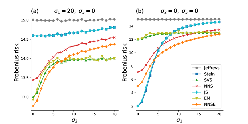
Figure 1: Frobenius risk functions of shrinkage estimators and generalized Bayes estimators when $m=3$, $n=5$.

Figure 2 compares the shrinkage estimators discussed in Section 2. Here, we only consider positive-part estimators because they dominate the corresponding shrinkage estimators. We also consider the positive-part modified Efron–Morris (mEM+) estimator proposed by Efron and Morris (1976):

$$\hat{\sigma}_{i}=\max\left(\sigma_{i}-\frac{n-m-1}{\sigma_{i}}-(m-1)(m+2)\frac{\sigma_{i}}{\sum_{j=1}^{m}\sigma_{j}^{2}},0\right),\quad i=1,\dots,m.$$

Figure 2 plots the risk functions with respect to $\sigma_{1}$ when $m=20$, $n=100$, $\sigma_{i}=(6-i)\sigma_{1}/5$ for $i=2,\dots,5$, and $\sigma_{6}=\cdots=\sigma_{20}=0$. When $\sigma_{1}$ is less than $10$, JS+ estimator performs the best. When $\sigma_{1}$ is in $[15,25]$, $M^{*,+}_{1}$ attains the best performance. When $\sigma_{1}$ is larger than $30$, $M^{*,+}_{\frac{1}{2}}$ outperforms other estimators.

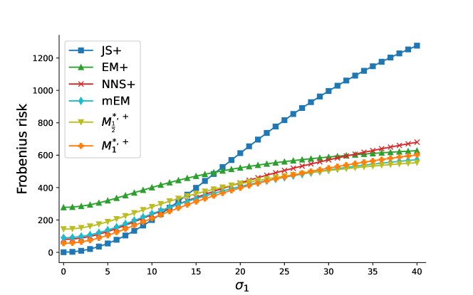
Figure 2: Frobenius risk functions of shrinkage estimators when $m=20$, $n=100$, $\sigma_{i}=(6-i)\sigma_{1}/5$ for $i=2,\dots,5$, and $\sigma_{6}=\cdots=\sigma_{20}=0$.

Table 1 presents the Frobenius risk on two types of low rank matrices. When $\sigma_{1}$ is small, JS+ has the best performance. When $\sigma_{1}$ is large, $\hat{M}^{*,+}_{\frac{1}{2}}$ has the best performance. It can be seen that $\hat{M}^{*,+}_{\frac{1}{2}}$ outperforms EM+ in all cases. Although the two estimators $\hat{M}^{*,+}_{1}$ and NNS+ have a similar form to the SVT estimator, $\hat{M}^{*,+}_{1}$ outperforms NNS+ in all cases.

Table 1: Frobenius risk of shrinkage estimators

	mEM+	EM+	$M^{*,+}_{\frac{1}{2}}$	NNS+	$M^{*,+}_{1}$	JS+
$n=20$, $m=15$, $\sigma_{1}=\cdots=\sigma_{10}$, $\sigma_{11}=\dots=\sigma_{15}=0$
$\sigma_{1}=1$	13.6	215.6	120.0	75.0	44.1	10.8*
$\sigma_{1}=10$	223.6*	268.7	243.9	239.4	232.1	231.5
$\sigma_{1}=100$	273.4	274.0	263.6*	294.7	282.5	299.1
$\sigma_{1}=1000$	274.1	274.1	263.0*	299.5	286.2	300.0
$n=100$, $m=20$, $\sigma_{i}=\sigma_{1}\max(1-(i-1)/5,0)$
$\sigma_{1}=1$	91.7	279.8	145.3	82.1	58.2	3.2*
$\sigma_{1}=10$	238.2	400.8	280.6	233.0	210.2	200.0*
$\sigma_{1}=100$	691.6	703.6	646.7*	1085.5	801.5	1833.5
$\sigma_{1}=1000$	728.8	728.9	662.2*	1842.2	958.0	1998.2
$\sigma_{1}=10000$	729.2	729.2	656.1*	1983.1	974.5	2000.0

Finally, we consider the prediction problem, where we predict $Y\sim\mathrm{N}(M,I_{n},I_{m})$ using $X\sim\mathrm{N}(M,I_{n},I_{m})$. We compare the Kullback–Leibler risk of the Bayesian predictive density $p_{\pi}(Y\mid X)$ based on the Jeffreys prior $\pi(M)\equiv 1$, Stein’s prior (1.3), singular value shrinkage prior (1.4), and the nuclear norm shrinkage prior (3.6). We sampled $(X,Y)$ $10^{5}$ times and approximated the Kullback–Leibler risk by the sample mean of $\log p(Y\mid M)-\log p_{\pi}(Y\mid X)$. We set $m=3$, $n=5$, and $\sigma_{3}=0$. Figure 3(a) shows the risk functions for $\sigma_{1}=20$. Figure 3(b) shows the risk functions for $\sigma_{2}=0$. We can see that all the priors outperform the Jeffreys prior. When all the singular values are close to zeros, Stein prior performs the best. When $\sigma_{1}$ and $\sigma_{2}$ are moderately large, the nuclear norm shrinkage prior performs the best. When $\sigma_{1}$ and $\sigma_{2}$ are large, the singular value shrinkage prior performs the best.

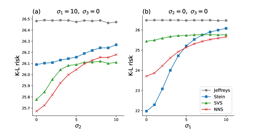
Figure 3: Kullback–Leibler risk functions of Bayesian predictive densities when $m=3$, $n=5$.

Appendix A Technical Lemmas

Lemma 1.

When $p\in(0,2]$, $(x^{p}-1)/(x^{2}-1)$ is a decreasing function of $x>1$ and a decreasing function of $x\in(0,1)$. Moreover, $(x^{p}-1)/(x^{2}-1)<p/2$ when $x>1$ and $(x^{p}-1)/(x^{2}-1)>p/2$ when $x\in(0,1).$

Proof.

The differential function is

$$\frac{(x^{p}-1)^{\prime}(x^{2}-1)-(x^{p}-1)(x^{2}-1)^{\prime}}{(x^{2}-1)^{2}}=\frac{(p-2)x^{p+1}-px^{p-1}+2x}{(x^{2}-1)^{2}}.$$

We define $g(x)=(p-2)x^{p}-px^{p-2}+2$. Then the differential function is $xg(x)/(x^{2}-1)^{2}$. We need only show that $g(x)\leq 0$ for any $x>0$. Note that $g(1)=0$ and

$$g(x)^{\prime}=(p-2)px^{p-1}-p(p-2)x^{p-3}=(2-p)px^{p-3}(1-x^{2}).$$

Thus, $g(x)\leq 0$.

Moreover, $\lim_{x\to 1}(x^{p}-1)/(x^{2}-1)=p/2$. Therefore, $(x^{p}-1)/(x^{2}-1)<p/2$ when $x>1$ and $(x^{p}-1)/(x^{2}-1)>p/2$ when $x\in(0,1).$ ∎

Lemma 2.

When $p\in[1,2]$ and $\sigma_{i},\ \sigma_{j}$ are different nonnegative numbers,

$$\frac{\sigma_{i}^{2p}-\sigma_{j}^{2p}}{\sigma_{i}^{2}-\sigma_{j}^{2}}\geq\frac{p}{2}(\sigma_{i}^{2p-2}+\sigma_{j}^{2p-2}).$$ (A.1)

Proof.

We need only show that $x^{2p}-1\geq p/2(x^{2p-2}+1)(x^{2}-1)$ for any $x\geq 1$. Define

$$g(x)=x^{2p}-1-p/2(x^{2p-2}+1)(x^{2}-1).$$

Then

$$g^{\prime}(x)=(2-p)px^{2p-1}-px+p(p-1)x^{2p-3}=:pxh(x),$$

where $h(x)=(2-p)x^{2p-2}-1+(p-1)x^{2p-4}$. Note that

$$h^{\prime}(x)=(2-p)(2p-2)x^{2p-3}-(p-1)(4-2p)x^{2p-5}=(2-p)(2p-2)(x^{2p-3}-x^{2p-5})\geq 0.$$

Thus, $h(x)\geq h(1)=0$. Thus, $g^{\prime}(x)=pxh(x)\geq 0$. Hence $g(x)\geq g(1)=0.$ ∎

Lemma 3.

(Chebyshev’s sum inequality) If $a_{1}\geq a_{2}\geq\cdots\geq a_{m}$ and $b_{1}\leq b_{2}\leq\cdots\leq b_{m}$, then

$$\Big{(}\sum_{i=1}^{m}a_{i}\Big{)}\Big{(}\sum_{i=1}^{m}b_{i}\Big{)}\geq m\sum_{i=1}^{m}a_{i}b_{i}.$$

Lemma 4.

When $p\in(0,2]$ and $\sigma_{1},\dots,\sigma_{m}$ are different nonnegative numbers,

$$\Big{(}\sum_{i=1}^{m}\sigma_{i}^{p}\Big{)}\sum_{i<j}\frac{\sigma_{i}^{p}-\sigma_{j}^{p}}{\sigma_{i}^{2}-\sigma_{j}^{2}}\geq\frac{m}{2}\sum_{i<j}\frac{\sigma_{i}^{2p}-\sigma_{j}^{2p}}{\sigma_{i}^{2}-\sigma_{j}^{2}}.$$

Proof.

For given $i$, using Lemma 1,

$$\frac{\sigma_{i}^{p}-\sigma_{j}^{p}}{\sigma_{i}^{2}-\sigma_{j}^{2}}=\sigma_{i}^{p-2}\frac{(\sigma_{j}/\sigma_{i})^{p}-1}{(\sigma_{j}/\sigma_{i})^{2}-1}$$

is a decreasing function of $\sigma_{j}$. Therefore, using $\sigma_{1}\geq\cdots\geq\sigma_{m}$, $(\sigma_{i}^{p}-\sigma_{j}^{p})/(\sigma_{i}^{2}-\sigma_{j}^{2})$ is a increasing function of $j$. For given $i$, $\sigma_{i}^{p}+\sigma_{j}^{p}$ is a decreasing function of $j$. Therefore, for given $i$, using Chebyshev’s sum inequality,

$$\Big{(}\sum_{j\neq i}(\sigma_{i}^{p}+\sigma_{j}^{p})\Big{)}\Big{(}\sum_{j\neq i}\frac{\sigma_{i}^{p}-\sigma_{j}^{p}}{\sigma_{i}^{2}-\sigma_{j}^{2}}\Big{)}\geq(m-1)\sum_{j\neq i}\frac{\sigma_{i}^{2p}-\sigma_{j}^{2p}}{\sigma_{i}^{2}-\sigma_{j}^{2}}.$$ (A.2)

For given $j$, using Lemma 1, $(\sigma_{i}^{p}-\sigma_{j}^{p})/(\sigma_{i}^{2}-\sigma_{j}^{2})$ is a decreasing function of $\sigma_{i}$. Therefore, if $\sigma_{i_{1}}\geq\sigma_{i_{2}}$,

$$\sum_{j\neq i_{1}}(\sigma_{i_{1}}^{p}-\sigma_{j}^{p})/(\sigma_{i_{1}}^{2}-\sigma_{j}^{2})-\sum_{j\neq i_{2}}(\sigma_{i_{2}}^{p}-\sigma_{j}^{p})/(\sigma_{i_{2}}^{2}-\sigma_{j}^{2})$$

is nonpositive. Therefore, using $\sigma_{1}\geq\cdots\geq\sigma_{m}$, $\sum_{j\neq i}(\sigma_{i}^{p}-\sigma_{j}^{p})/(\sigma_{i}^{2}-\sigma_{j}^{2})$ is a increasing function of $i$. In addition, $\sum_{j\neq i}(\sigma_{i}^{p}+\sigma_{j}^{p})=\sum_{j}\sigma_{j}^{p}+(m-2)\sigma_{i}^{p}$ is a decreasing function of $i$. Therefore, using Chebyshev’s sum inequality,

$$\Big{(}\sum_{i=1}^{m}\sum_{j\neq i}(\sigma_{i}^{p}+\sigma_{j}^{p})\Big{)}\Big{(}\sum_{i=1}^{m}\sum_{j\neq i}\frac{\sigma_{i}^{p}-\sigma_{j}^{p}}{\sigma_{i}^{2}-\sigma_{j}^{2}}\Big{)}\geq m\sum_{i=1}^{m}\Big{(}\sum_{j\neq i}(\sigma_{i}^{p}+\sigma_{j}^{p})\Big{)}\Big{(}\sum_{j\neq i}\frac{\sigma_{i}^{p}-\sigma_{j}^{p}}{\sigma_{i}^{2}-\sigma_{j}^{2}}\Big{)}.$$ (A.3)

Combining (A.2) and (A.3), we have

$$\Big{(}\sum_{i=1}^{m}\sigma_{i}^{p}\Big{)}\sum_{i<j}\frac{\sigma_{i}^{p}-\sigma_{j}^{p}}{\sigma_{i}^{2}-\sigma_{j}^{2}} =\frac{1}{4(m-1)}\Big{(}\sum_{i=1}^{m}\sum_{j\neq i}(\sigma_{i}^{p}+\sigma_{j}^{p})\Big{)}\Big{(}\sum_{i=1}^{m}\sum_{j\neq i}\frac{\sigma_{i}^{p}-\sigma_{j}^{p}}{\sigma_{i}^{2}-\sigma_{j}^{2}}\Big{)}$$

$$\geq\frac{m}{4(m-1)}\sum_{i=1}^{m}\Big{(}\sum_{j\neq i}(\sigma_{i}^{p}+\sigma_{j}^{p})\Big{)}\Big{(}\sum_{j\neq i}\frac{\sigma_{i}^{p}-\sigma_{j}^{p}}{\sigma_{i}^{2}-\sigma_{j}^{2}}\Big{)}$$

$$\geq\frac{m}{4}\sum_{i=1}^{m}\sum_{j\neq i}\frac{\sigma_{i}^{2p}-\sigma_{j}^{2p}}{\sigma_{i}^{2}-\sigma_{j}^{2}}=\frac{m}{2}\sum_{i<j}\frac{\sigma_{i}^{2p}-\sigma_{j}^{2p}}{\sigma_{i}^{2}-\sigma_{j}^{2}}.$$

∎

Lemma 5.

When $p\in[1,2]$ and $\sigma_{1},\dots,\sigma_{m}$ are different nonnegative numbers,

$$\Big{(}\sum_{i=1}^{m}\sigma_{i}^{p}\Big{)}\sum_{i<j}\frac{\sigma_{i}^{p}-\sigma_{j}^{p}}{\sigma_{i}^{2}-\sigma_{j}^{2}}\geq\frac{pm(m-1)}{4}\sum_{i=1}^{m}\sigma_{i}^{2p-2}.$$

Proof.

Combining Lemmas 2 and 4, we have

$$\Big{(}\sum_{i=1}^{m}\sigma_{i}^{p}\Big{)}\sum_{i<j}\frac{\sigma_{i}^{p}-\sigma_{j}^{p}}{\sigma_{i}^{2}-\sigma_{j}^{2}} \geq\frac{m}{2}\sum_{i<j}\frac{\sigma_{i}^{2p}-\sigma_{j}^{2p}}{\sigma_{i}^{2}-\sigma_{j}^{2}}$$

$$\geq\frac{pm}{4}\sum_{i<j}(\sigma_{i}^{2p-2}+\sigma_{j}^{2p-2})=\frac{pm(m-1)}{4}\sum_{i=1}^{m}\sigma_{i}^{2p-2}.$$

∎

References

Aitchison (1975)Aitchison, J. 1975.
Goodness of prediction fit.
Biometrika62, 3, 547–554.
Cai et al. (2010)Cai, J.-F., Candès, E. J., andShen, Z. 2010.
A singular value thresholding algorithm for matrix completion.
SIAM Journal on optimization20, 4, 1956–1982.
Candes et al. (2013)Candes, E. J., Sing-Long, C. A., andTrzasko, J. D. 2013.
Unbiased risk estimates for singular value thresholding and spectral estimators.
IEEE transactions on signal processing61, 19, 4643–4657.
Efron and Morris (1972)Efron, B.andMorris, C. 1972.
Empirical bayes on vector observations: An extension of stein’s method.
Biometrika59, 2, 335–347.
Efron and Morris (1976)Efron, B.andMorris, C. 1976.
Multivariate empirical bayes and estimation of covariance matrices.
The Annals of Statistics, 22–32.
George et al. (2006)George, E. I., Liang, F., andXu, X. 2006.
Improved minimax predictive densities under kullback-leibler loss.
The Annals of Statistics, 78–91.
Helms (2009)Helms, L. L. 2009.
Potential Theory.
Springer London.
James and Stein (1961)James, W.andStein, C. 1961.
Estimation with quadratic loss.
In Proceedings of the Fourth Berkeley Symposium on Mathematical Statistics and Probability, Volume 1: Contributions to the Theory of Statistics. Vol. 4. University of California Press, 361–379.
Komaki (2001)Komaki, F. 2001.
A shrinkage predictive distribution for multivariate normal observables.
Biometrika88, 3, 859–864.
Matsuda and Komaki (2015)Matsuda, T.andKomaki, F. 2015.
Singular value shrinkage priors for bayesian prediction.
Biometrika102, 4, 843–854.
Matsuda and Strawderman (2019)Matsuda, T.andStrawderman, W. E. 2019.
Improved loss estimation for a normal mean matrix.
Journal of Multivariate Analysis169, 300–311.
Matsuda and Strawderman (2022)Matsuda, T.andStrawderman, W. E. 2022.
Estimation under matrix quadratic loss and matrix superharmonicity.
Biometrika109, 2, 503–519.
Stein (1974)Stein, C. M. 1974.
Estimation of the mean of a multivariate normal distribution.
In Proc. Prague Symposium on Asymptotic Statistics (J. Hájek, ed.). Vol. 2. Univ. Karlova, Prague, 345–381.
Tsukuma (2008)Tsukuma, H. 2008.
Admissibility and minimaxity of bayes estimators for a normal mean matrix.
Journal of multivariate analysis99, 10, 2251–2264.
Tsukuma and Kubokawa (2017)Tsukuma, H.andKubokawa, T. 2017.
Proper bayes and minimax predictive densities related to estimation of a normal mean matrix.
Journal of Multivariate Analysis159, 138–150.
Yuasa and Kubokawa (2023)Yuasa, R.andKubokawa, T. 2023.
Weighted shrinkage estimators of normal mean matrices and dominance properties.
Journal of Multivariate Analysis194, 105138.