Model Updating for Nonlinear Systems
with Stability Guarantees

Abstract.

To improve the predictive capacity of system models in the input-output sense, this paper presents a framework for model updating via learning of modeling uncertainties in locally (and thus also in globally) Lipschitz nonlinear systems. First, we introduce a method to extend an existing known model with an uncertainty model so that stability of the extended model is guaranteed in the sense of set invariance and input-to-state stability. To achieve this, we provide two tractable semi-definite programs. These programs allow obtaining optimal uncertainty model parameters for both locally and globally Lipschitz nonlinear models, given uncertainty and state trajectories. Subsequently, in order to extract this data from the available input-output trajectories, we introduce a filter that incorporates an approximated internal model of the uncertainty and asymptotically estimates uncertainty and state realizations. This filter is also synthesized using semi-definite programs with guaranteed robustness with respect to uncertainty model mismatches, disturbances, and noise. Numerical simulations for a large data-set of a roll plane model of a vehicle illustrate the effectiveness and practicality of the proposed methodology in improving model accuracy, while guaranteeing stability.

1. Introduction

Dynamical systems modeling has been a key problem in many engineering and scientific fields, such as biology, physics, chemistry, and transportation. When modeling dynamical systems, it is of key importance to use well-established principles of physics and known prior system properties (e.g., stability and set-invariance) [manchester2021contraction]. However, for many complex practical systems, we only tend to have partial knowledge of the physics governing their dynamics [abbasi2022physics]. Even in cases where accurate physics-based models are established, as, e.g., in robotics, there exist inevitable (both parametric and non-parametric) uncertainties that impact the model’s predictive accuracy.

For a class of nonlinear dynamical systems, this paper assumes a prior system model is available (however, results here are also applicable when no prior model is available). It focuses on learning models for uncertainties while guaranteeing the stability of extended models (prior models plus uncertainty representations), given available input-output data. This problem contrasts with black box modeling approaches, such as Neural Networks (NNs) or Gaussian Processes (GPs), because we incorporate prior relationships derived from first principles into both the modeling and learning framework. Moreover, this problem differs from typical grey-box identification problems because, in our case, a prior model with known parameters is available. Off-the-shelf grey-box system identification methods can cope with a subset of the problem under discussion, where no prior model is available. The problem considered here enables the characterization of hybrid system representations (referred here as the extended model) comprising both prior physics-based and uncertainty learned models. In what follows, a comparison of our approach with some related existing literature on hybrid modeling (based on both first-principles and data) is provided.

Existing Literature: Our approach is fundamentally different from existing Physics-Informed (PI) learning techniques where standard black box models (such as NNs or GPs) are trained constrained to satisfy physics-based relations [yazdani2020systems, daneker2023systems, taneja2022feature]. Yazdani et al. in [yazdani2020systems] use this technique to construct the so-called Physics Informed Neural Networks (PINNs). They constrain a known physics-based model during the training of a NN-based model (i.e., penalize loss function for the mismatch between the physics-based model and the NN as a soft constraint) and incorporate physics knowledge in the structure of the NN. Although this method provides a NN as a system model (as well as parameters for physics-based models), it does not give a closed-form expression for the uncertainty in known physics-based models (i.e., it does not account for modeling mismatches due to unmodeled physics). Furthermore, parameters of both physics-based models and NNs are learned simultaneously, which increases the computational burden.

The approach proposed in this paper also differs from the so-called Sparse Identification of Nonlinear Dynamics (SINDy) scheme [brunton2016discovering]. SINDy assumes full knowledge of system states and their time derivatives. Then, based on known physics-based models and known variables (i.e., system states and their derivatives) a library of functions is generated that can be incorporated in dynamical models to account for uncertainty. To select the active functions in models, sparse identification algorithms are exploited. This approach has demonstrated accurate performance in sparse model identification of complex nonlinear systems [champion2019data, champion2020unified, loiseau2018constrained]. However, SINDy not only requires full-state measurement but also requires the derivative of states to be known. Although the state derivatives can be approximated numerically if the complete state is known, most numerical methods are noise sensitive. Furthermore, the requirement of full-state measurements is a strong assumption for most dynamical systems. In our work, we do not require measurements of the full-state and its time derivative. The proposed algorithms need input-output data only.

Our approach augments a known physics-based model by a black-box model used as a correction term, see, e.g., [schneider2022hybrid, bradley2022perspectives] and references therein. Such generic approach is also taken by Quaghebeur et al. in [quaghebeur2021incorporating], who add an NN model to a known physics-based model with unknown parameters. This approach allows maintaining the basic structure of the model that comes from first principles, which improves interpretability. However, simulating the hybrid model at each iteration during the training process is necessary. This approach is evidently more computationally intensive compared to our proposed method, which eliminates the requirement of simulating the model in every iteration. Moreover, the main drawback of this method is that it assumes that the initial state of the dynamic system is known or at least it requires measuring all the states (full-state measurement) of the true dynamical system. This assumption is dropped in the proposed method considered here.

Another important advantage of the proposed method is guaranteeing the stability of the extended nonlinear model (i.e., the model consisting of the known physics-based model and the uncertainty model). The identification of stable models has (mainly) been widely studied in the context of discrete LTI systems [lacy2003subspace, di2023simba]. For further results on uncertainty learning for LTI systems, refer to [ghanipoor2023uncertainty]. However, the identification of nonlinear stable models is still under study, mainly focusing on identifying the complete dynamics in a black box fashion. For instance, kernel- or Koopman-based methods that enforce some form of model stability during the learning process are proposed in [khosravi2020nonlinear, khosravi2023representer] for the autonomous case and for the non-autonomous case in [shakib2023kernel]. Moreover, there are results that aim to enforce model stability in other types of models, such as recurrent equilibrium network models [revay2021recurrent] and Lur’e-type models [shakib2019fast, revay2023recurrent]. However, it is important to note that none of these methods can be directly applied to the specific problem we are addressing here, given the prior known model.

In this paper, we propose a framework for model updating via learning modeling uncertainties in (physics-based) models applicable to locally Lipschitz nonlinear systems. We first focus on learning uncertainty models, assuming that some realizations of input, estimated uncertainty, and estimated state are given. During uncertainty learning, we guarantee that trajectories of the extended model (i.e., known prior model plus uncertainty model) belong to a given invariant set for locally Lipschitz extended models, or ensure input-to-state stability for globally Lipschitz extended models. This is achieved by formulating the problem as a constrained supervised learning problem.

One key challenge in this problem involves the introduction of stability constraints, which is tackled using Lyapunov-based tools. The stability criteria usually result in an optimization problem that is non-convex. We address this challenge by proposing two different approaches for both locally and globally Lipschitz models:

1. Cost Modification: The first approach involves a change of variables, which leads to the rewriting of cost function (Theorems 3.1 and LABEL:theorem:learning_modified_cost_globally for locally and globally Lipschitz models, respectively).

2. Constraint Modification: This approach introduces a sufficient (convex) condition to satisfy the stability constraint (Theorems LABEL:theorem:learning_modified_constraint_locally and LABEL:theorem:learning_modified_constraint_globally for locally and globally Lipschitz models, respectively).

For the sake of completeness and comparison, we also provide a sequential algorithm that alternates the use of some variables in the optimization problem to convexity the program. However, we show in the numerical section that (as it is known in related literature [boyd1994linear]) that initializing this algorithms is challenging, which further strengthens the importance of the results provided here. We referred to the above mentioned sequential algorithm as the method of Sequential Convex Programming (SCP).

After addressing the challenge of non-convexity, the paper proceeds to discuss the practical implementation of the framework. It outlines a method for estimating uncertainty and state trajectories using input-output data and the known prior model (Proposition LABEL:prop:optimal_estimator). In this context, uncertainty is considered as an unknown input affecting the system dynamics and the estimation of uncertainty and state trajectories is achieved using robust state and unknown input observers [ghanipoor2023robust]. For a schematic overview of the proposed methodology, Model Updating for Nonlinear Systems with Stability guarantees (MUNSyS), see Figure 1.

Figure 1. Overview of the MUNSyS methodology.

In summary, the main contributions of this paper are as follows:

1. Practically Applicable Framework: The proposed framework for learning modeling uncertainties in locally (and globally) Lipschitz nonlinear models only requires input-output data. Another important aspect for practical applicability is the lower computational cost compared to existing methods. This is achieved by eliminating the requirement to simulate the model in every iteration.

2. Stability Guarantee of Extended Models: The proposed framework guarantees the following: 1. For locally Lipschitz extended models, trajectories of the extended model (i.e., known prior model plus uncertainty model) belong to a given invariant set; 2. For globally Lipschitz models, it ensures Input-to-State Stability (ISS).

3. Convex Approximations for Non-Convex Programs: Two distinct approaches for both locally and globally Lipschitz models, namely cost and constraint modification, are proposed to offer tractable convex approximations of formulated non-convex optimization problems for uncertainty model learning, while ensuring stability guarantees.

This paper generalizes the preliminary results published in the conference paper [ghanipoor2023uncertainty]. In comparison to [ghanipoor2023uncertainty], which is applicable to LTI systems only, we present results for a broader class of systems, considering both locally and globally Lipschitz nonlinear systems. The results in [ghanipoor2023uncertainty] are a subclass of the results provided for globally Lipschitz nonlinear systems (see Theorem LABEL:theorem:learning_modified_cost_globally).

Notation: The set of nonnegative real numbers is represented by the symbol $\mathbb{R}^{+}$. The identity matrix of size $n\times n$ is denoted as $I_{n}$ or simply $I$ when the context specifies $n$. Similarly, matrices of dimensions $n\times m$ comprising only zeros are denoted as ${0}_{n\times m}$ or ${0}$ when the dimensions are clear. The first and second time-derivatives of a vector $x$ are denoted as $\dot{x}$ and $\ddot{x}$, respectively. For the $r^{th}$-order time-derivatives of vector $x$, the notation $x^{(r)}$ is employed. A positive definite matrix is symbolized by $X\succ 0$, and positive semi-definite matrices are indicated by $X\succeq 0$. Similarly, $X\prec 0$ is used for negative definite matrices, and $X\preceq 0$ for negative semi-definite matrices. The Hadamard (element-wise) power of $n\in\mathbb{N}$ for a matrix $X$ is denoted by $X^{\circ n}$. The same notation is used for vectors. The $exp(x)$ shows the element-wise exponential function. The notation $(x_{1},\ldots,x_{n})$ signifies the column vector composed of elements $x_{1},\ldots,x_{n}$, and this notation is also used when the components $x_{i}$ are vectors. Both Euclidean norm and the matrix norm induced by Euclidean norm are represented by the notation $||\cdot||$. The infinity-norm is denoted as $||\cdot||_{\infty}$. We employ the notation $\mathcal{L}_{2}(0,T)$ (or simply $\mathcal{L}_{2}$) to represent vector-valued functions $z:[0,T]\to\mathbb{R}^{k}$ satisfying $||z(t)||_{\mathcal{L}_{2}}^{2}:=\int_{0}^{T}||z(t)||^{2}dt<\infty$. For a vector-valued signal $z$ defined for all $t\geq 0$, the $\mathcal{L}_{\infty}$ norm is denoted as $||z||_{\mathcal{L}_{\infty}}:=\sup_{t\geq 0}||z(t)||$. For a differentiable function $V:\mathbb{R}^{n}\to\mathbb{R}$, the row-vector of partial derivatives is denoted as $\frac{\partial V}{\partial x}$, and $\dot{V}(x)$ denotes the total derivative of $V(x)$ with respect to time (i.e., $\frac{\partial V}{\partial x}\frac{dx}{dt}$). The trace of a matrix $W$ is denoted as $tr(W)$. A continuous function $\bar{\alpha}:[0,a)\rightarrow[0,\infty)$ is said to belong to class $\mathcal{K}$ if it is strictly increasing and $\bar{\alpha}(0)=0$. A continuous function $\bar{\beta}:[0,a)\times[0,\infty)\rightarrow[0,\infty)$ is said to belong to class $\mathcal{KL}$ if, for each fixed $s$, the mapping $\bar{\beta}(r,s)$ belongs to class $\mathcal{K}$ with respect to $r$ and, for each fixed $r$, the mapping $\bar{\beta}(r,s)$ is decreasing with respect to $s$ and $\bar{\beta}(r,s)\rightarrow 0$ as $s\rightarrow\infty$. Time dependencies are often omitted for simplicity in notation.

2. Problem Formulation

Consider the nonlinear system

$$\left\{\begin{aligned} \dot{x}_{s}&=Ax_{s}+B_{u}u+S_{g}g(V_{g}x_{s},u)+S_{\eta}\eta(V_{\eta}x_{s},u)+B_{\omega}\omega,\\ y_{s}&=Cx_{s}+D_{\nu}\nu,\end{aligned}\right.$$ (1)

where $x_{s}\in{\mathbb{R}^{n}}$, $y_{s}\in{\mathbb{R}^{{m}}}$, and $u\in{\mathbb{R}^{{l}}}$ are system state, measured output and known input vectors, respectively. Function $g:\mathbb{R}^{n_{v_{g}}}\times\mathbb{R}^{l}\to\mathbb{R}^{n_{g}}$ is a known nonlinear vector field, and function $\eta:\mathbb{R}^{n_{v_{\eta}}}\times\mathbb{R}^{l}\to\mathbb{R}^{n_{\eta}}$ denotes unknown modeling uncertainty. Signals $\omega:\mathbb{R}^{+}\to\mathbb{R}^{n_{\omega}}$ and $\nu:\mathbb{R}^{+}\to\mathbb{R}^{m_{\nu}}$ are unknown bounded disturbances; the former with unknown frequency range and the latter typically with high-frequency content (e.g., related to measurement noise). Known matrices $(A,B_{u},S_{g},V_{g},S_{\eta},V_{\eta},B_{\omega},C,D_{\nu})$ are of appropriate dimensions, with ${n},{m},l,n_{v_{g}},n_{g},n_{v_{\eta}},n_{\eta},n_{\omega},m_{\nu}\in\mathbb{N}$. The matrices $S_{g}$ and $S_{\eta}$ specify the equations explicitly incorporating the nonlinearity $g$ and uncertainty $\eta$, while the matrices $V_{g}$ and $V_{\eta}$ identify the states influencing the nonlinearity and uncertainty, respectively. Moreover, without loss of generality, we assume that zero is an equilibrium point of the system for $u=0$.

In the following, we state the problem we aim to solve at a high abstraction level.

Problem 1.

(Uncertainty Learning with Stability Guarantees) Consider system (1) with known input and output signals, $u$ and $y_{s}$. We aim to learn a data-based model for the uncertainty function $\eta(\cdot)$ so that the extended model composed of the known part of (1) and the learned uncertainty model are “stable”. The objective is to construct a more accurate system model (at least applicable to trajectories close to the training data set).

We first assume the availability of a labeled data-set containing input, estimated uncertainty, and estimated state realizations. A method to obtained this data from input-output trajectories is given in Section LABEL:sec:_uncertainty_state_estimation. In what follows, we outline the problem settings for both locally and globally Lipschitz systems.

2.1. Problem Settings

We consider two model classes. For both model classes, the extended model (for the system in (1)) is of the form:

$$\dot{x} =Ax+B_{u}u+S_{g}g(V_{g}x,u)+S_{\eta_{l}}\eta_{l}(V_{\eta}x,u),$$ (2)

$$\eta_{l}(V_{\eta}x,u) :=\Theta_{l}V_{\eta}x+B_{l}u+\Theta_{n}h(V_{\eta}x,u),$$

where $x\in{\mathbb{R}^{n}}$ is model state and function $\eta_{l}:\mathbb{R}^{n_{v_{\eta}}}\times\mathbb{R}^{l}\to\mathbb{R}^{n_{\eta_{l}}}$ is the uncertainty model that is parameterized by $\Theta_{l},B_{l}$ and $\Theta_{n}$. Function $h:\mathbb{R}^{n_{v_{\eta}}}\times\mathbb{R}^{l}\to\mathbb{R}^{n_{h}}$ is a given nonlinear vector filed. This function contains the vector of basis functions that serve as candidates for the nonlinearities in the uncertainty model. Design matrices are collected as $\theta=(\Theta_{l},B_{l},\Theta_{n})$ and have appropriate dimensions, $n_{\eta_{l}},n_{h}\in\mathbb{N}$. Matrix $S_{\eta_{l}}$, similar to $S_{\eta}$ in (1), indicates the explicit presence of the uncertainty model $\eta_{l}$ in the right-hand side and may differ from $S_{\eta}$.

2.1.1. Cost Function

Recall that, for now, we assume that estimated uncertainty and state realizations are available. Define the data vector corresponding to the $i$-th sample in time as

$$d_{i}:={\left[\begin{array}[]{cccc}\hat{x}_{i}^{\top}V_{\eta}^{\top}&u_{i}^{\top}&\hat{\eta}_{i}^{\top}&h(V_{\eta}\hat{x}_{i},u_{i})^{\top}\end{array}\right]^{\top}},$$

where $\hat{x}_{i},u_{i},$ and $\hat{\eta}_{i}$ represent the state estimate, input, and uncertainty estimate, respectively. Vector $h(V_{\eta}\hat{x}_{i},u_{i})$ corresponds to the evaluated nonlinearity in (2) at the given realizations (of state estimation and input). Given $N$ samples of the data vector defined above, define the data matrix $D$ as follows:

$$D:=\sum_{i=1}^{N}d_{i}d_{i}^{\top}.$$ (3)

Further, consider the error vector between the uncertainty model and its (given) estimate as

$$e_{i}:=\eta_{l}(V_{\eta}\hat{x}_{i},u_{i})-\hat{\eta}_{i}=Td_{i},\quad\text{where}\quad T:={\left[\begin{array}[]{cccc}\Theta_{l}&B_{l}&-I&\Theta_{n}\end{array}\right]}.$$ (4)

Next, we introduce the following quadratic cost function to be minimized for the identification of $\Theta_{l}$, $B_{l}$, and $\Theta_{n}$:

$$J:=\sum_{i=1}^{N}e_{i}^{\top}e_{i}=\sum_{i=1}^{N}d_{i}^{\top}T^{\top}Td_{i}.$$ (5)

In the following sections, for two model classes, we provide stability constraints and formulate the constrained supervised learning of uncertainty models as optimization problems.

2.1.2. Locally Lipschitz Model Class

We first consider locally Lipschitz nonlinearities in (2), for both the basis functions $h(\cdot)$ and the known vector field $g(\cdot)$. Note that given bounded estimated state and input trajectories, we can always find ellipsoids that bound these trajectories. Hereafter, the system state and input trajectories are referred to as state and input sets, respectively.

Note that the set of all trajectories that can be generated by system in (1) is not known a priori. We only have finite data realizations of the estimated state in response to some input trajectories. Given this, we seek models (2) that generate state trajectories “close” to the available data set in response to inputs “close” to the known input trajectories. To this end, we embed estimated state data and input trajectories in some known ellipsoidal sets, $\mathcal{E}_{sys}$ and $\mathcal{E}_{u}$, respectively. This embedding can be obtained efficiently, e.g., exploiting results in [boyd1994linear, Sec. 2.2.4].

Having these ellipsoids $\mathcal{E}_{sys}$ and $\mathcal{E}_{u}$, to induce closeness of trajectories between system training data and model trajectories, we seek to enforce during learning that all trajectories generated by the model, in response to all input trajectories contained in $\mathcal{E}_{u}$, are contained in some known ellipsoidal set $\mathcal{E}_{inv}$. If we enforce the latter, and $\mathcal{E}_{inv}\subseteq\mathcal{E}_{sys}$, then we can guarantee that the model produces trajectories close to the training date set (close in the sense of set inclusion within $\mathcal{E}_{sys}$), see Figure 2.

Let the ellipsoidal set containing the state estimates training data be of the form:

$$\mathcal{E}_{sys}:=\left\{x_{s}\mid x_{s}^{\top}Fx_{s}\leq 1\right\},$$ (6)

with $F\succeq 0$ of appropriate dimensions, and the input set of the form:

$$\mathcal{E}_{u}:=\left\{u\mid u^{\top}Uu\leq 1\right\},$$ (7)

with $U\succeq 0$ of appropriate dimension.

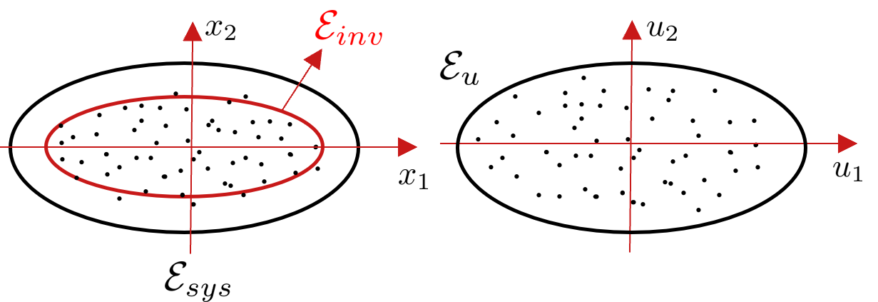
Figure 2. Illustration of different (ellipsoidal) sets for the system state $\mathcal{E}_{sys}$, input $\mathcal{E}_{u}$, and model state $\mathcal{E}_{inv}$.

Because we seek to restrict model trajectories to the sets $\mathcal{E}_{u}$ and $\mathcal{E}_{sys}$, and consider models in (2) with Lipschitz nonlinearities, we only require them to be Lipschitz within these sets. We formally state this in the following assumption.

Assumption 1.

(Locally Lipschitz Nonlinearities) The functions $g(V_{g}x,u)$ and $h(V_{\eta}x,u)$ in (2) are locally Lipschitz in $\mathcal{E}_{u}$ and $\mathcal{E}_{sys}$, i.e., there exist known positive constants $l_{g_{x}},l_{g_{u}},l_{h_{x}}$ and $l_{h_{u}}$ satisfying

$$\|g(V_{g}x_{1},u_{1})-g(V_{g}x_{2},u_{2})\| \leq l_{g_{x}}\|V_{g}(x_{1}-x_{2})\|+l_{g_{u}}\|u_{1}-u_{2}\|\,$$ (8)

$$\|h(V_{\eta}x_{1},u_{1})-h(V_{\eta}x_{2},u_{2})\| \leq l_{h_{x}}\|V_{\eta}(x_{1}-x_{2})\|\ +l_{h_{u}}\|u_{1}-u_{2}\|$$

for all $x_{1},x_{2}\in\mathcal{E}_{sys}\subset\mathbb{R}^{n}$ and all ${u_{1},u_{2}}\in\mathcal{E}_{u}\subset\mathbb{R}^{l}$.

In what follows, we formulate conditions to guarantee that model trajectories of (2), with locally Lipschitz nonlinearities, belong, in forward time, to an ellipsoidal invariant set:

$$\mathcal{E}_{inv}:=\left\{x\mid x^{\top}Px\leq 1\right\},$$ (9)

guaranteeing $\mathcal{E}_{inv}\subseteq\mathcal{E}_{sys}$, for some positive definite matrix $P$. Conditions to ensure the latter can be formulated through Lyapunov-based stability tools and the S-procedure [boyd1994linear, Sec. 2.6.3]. For the sake of readability, these conditions are derived in Appendix LABEL:ap:invariance_condtions. There, it is shown that if the following conditions hold, the ellipsoid $\mathcal{E}_{inv}$ is a forward invariant set for (2) and $\mathcal{E}_{inv}\subseteq\mathcal{E}_{sys}$:

$$\left[\begin{array}[]{ccc}\Delta+\beta P&P(B_{u}+S_{\eta_{l}}B_{l})&0\\ \star&(l_{g_{u}}+\bar{l}_{h_{u}})I-\alpha U&0\\ \star&\star&(\alpha-\beta)I\end{array}\right]\preceq 0,$$ (10d)

$$\left[\begin{array}[]{cc}\gamma F-P&0\\ &-\gamma+1\end{array}\right]\preceq 0,$$ (10g)

$$l_{h_{x}}\|\Theta_{n}\|\leq\bar{l}_{h_{x}},$$ (10h)

where the involved components in the above equation are defined as

$$\Delta :=A^{\top}P+PA+V_{\eta}^{\top}\Theta_{l}^{\top}S_{\eta_{l}}^{\top}P+PS_{\eta_{l}}\Theta_{l}V_{\eta}+(l_{g_{x}}+l_{g_{u}})PS_{g}S_{g}^{\top}P+(\bar{l}_{h_{x}}+\bar{l}_{h_{u}})PS_{\eta_{l}}S_{\eta_{l}}^{\top}P$$ (10i)

$$+l_{g_{x}}V_{g}^{\top}V_{g}+\bar{l}_{h_{x}}V_{\eta}^{\top}V_{\eta},$$

$$\bar{l}_{h_{u}} :=\bar{l}_{h_{x}}\frac{l_{h_{u}}}{l_{h_{x}}},$$ (10j)

and $\bar{l}_{h_{x}},\alpha,\beta,\gamma$ are adjustable parameters. In fact, $\bar{l}_{h_{x}}$ characterizes the size of a set within which $\Theta_{n}$ is enforced to reside.

Note that the condition in (10d) is not convex in the invariant set shape matrix $P$ and uncertainty model parameters $\theta=(\Theta_{l},B_{l},\Theta_{n})$, resulting in a non-convex optimization problem for uncertainty learning with invariance guarantees. Now, we can state the non-convex optimization problem for the locally Lipschitz model class, aiming to find a tractable convex solution later.

Problem Setting 1.

(Locally Lipschitz Model Class) Consider a given data-set $D$ of input, estimated uncertainty, and state realizations and let Assumption 1 be satisfied. Further consider given ellipsoidal sets $\mathcal{E}_{sys}$ and $\mathcal{E}_{u}$, as introduced in (6) and (7), respectively, containing the available input and state estimates data sets. Find the optimal parameters $\theta=(\Theta_{l},B_{l},\Theta_{n})$ of the uncertainty model $\eta_{l}(\cdot)$ in (2) (with locally Lipschitz nonlinearities) that minimizes the cost function $J$ in (5) constrained to the ellipsoid $\mathcal{E}_{inv}$ in (9) being a forward invariant set for the extended system model in (2). In other words, solve the non-convex optimization problem: —s— P,Θ_l, B_l,Θ_n, α, γ &J &(10)  and  P≻0.

In what follows, we formulate an analogue problem for the globally Lipschitz model class (that is assuming that the nonlinearities in (2) are globally Lipschitz).

Remark 1.

(Comparison of Locally and Globally Lipschitz Model Classes) The main drawback of the globally Lipschitz model class is that it covers a smaller class of nonlinear systems compared to the locally Lipschitz class. However, we can enforce a stronger stability property (input-to-state stability [sontag1995input]) for globally Lipschitz nonlinearities. Notably, for this model class, knowledge of the system state and input sets is no longer required. Furthermore, in the derivation of stability conditions for globally Lipschitz case, the need for a sufficient approximation (see S-procedure tools in Appendix LABEL:ap:invariance_condtions) is eliminated. This elimination relaxes the conservatism typically introduced by the sufficient condition. Moreover, the absence of this condition reduces the number of tuning parameters required for optimizing the globally Lipschitz class. The above arguments motivate to consider both model classes.

2.1.3. Globally Lipschitz Model Class

For this model class, the nonlinearities in (2) are assumed globally Lipschitz.

Assumption 2.

(Globally Lipschitz Nonlinearities) The functions $g(V_{g}x,u)$ and $h(V_{\eta}x,u)$ in (2) are globally Lipschitz, i.e., there exist known positive constants $l_{g_{x}},l_{g_{u}},l_{h_{x}}$ and $l_{h_{u}}$ satisfying

$$\|g(V_{g}x_{1},u_{1})-g(V_{g}x_{2},u_{2})\| \leq l_{g_{x}}\|V_{g}(x_{1}-x_{2})\|+l_{g_{u}}\|u_{1}-u_{2}\|,$$ (11)

$$\|h(V_{\eta}x_{1},u_{1})-h(V_{\eta}x_{2},u_{2})\| \leq l_{h_{x}}\|V_{\eta}(x_{1}-x_{2})\|+l_{h_{u}}\|u_{1}-u_{2}\|,$$

for all $x_{1},x_{2}\in{\mathbb{R}^{n}}$ and all ${u_{1},u_{2}}\in{\mathbb{R}^{l}}$.

In what follows, we formulate conditions to ensure Input-to-State Stability (ISS) of the extended model in (2) satisfying Assumption 2. In the following definition, we introduce the notion of ISS for the extended model [sontag1995input].

Definition 1.

(Input-to-State Stability) The extended model (2) is said to be ISS with respect to the input $u(t)$ if there exist a class $\mathcal{K}\mathcal{L}$ function $\bar{\beta}(\cdot)$ and a class $\mathcal{K}$ function $\bar{\alpha}(\cdot)$ such that for any initial state $x(t_{0})$ and any bounded input $u(t)$, the solution $x(t)$ of (2) exists for all finite $t\geq t_{0}$ and satisfies

$$\|x(t)\|\leq\bar{\beta}\left(\left\|x\left(t_{0}\right)\right\|,t-t_{0}\right)+\bar{\alpha}(\sup_{t_{0}\leq\tau\leq t}\|u(\tau)\|).$$ (12)

For readability, ISS conditions for the model in (2) satisfying Assumption 2 are derived in Appendix LABEL:ap:iss_condtions. It is shown that if the condition (10h) together with the following condition hold,

$$\Delta\prec 0,$$ (13)

where $\Delta$ is as defined in (10i), then, the extended model in (2) with globally Lipschitz nonlinearities is ISS with respect to the input $u(t)$.

Now, we can state the non-convex optimization problem for the globally Lipschitz model class, aiming to find a tractable convex approximation later.

Problem Setting 2.

(Globally Lipschitz Model Class) Consider a given data-set $D$ of input, estimated uncertainty, and state realizations and let Assumption 2 be satisfied. Find the optimal parameters $\theta=(\Theta_{l},B_{l},\Theta_{n})$ of the uncertainty model $\eta_{l}(\cdot)$ in (2) (with globally Lipschitz nonlinearities) that minimizes the cost function $J$ in (5), such that the extended system model in (2) is ISS with respect to input $u(t)$. In other words, solve the non-convex optimization problem: —s— P,Θ_l, B_l,Θ_n &J &(10h), (13), P≻0.

The challenge in Problem Settings 1 and 2 is that stability constraints are not convex, resulting in non-convex optimization problems. To tackle this challenge, we provide two approximate convex solutions for both problem settings using two distinct approaches: first, cost modification approach and second, constraint modification approach. Moreover, as an alternative solution, we provide a procedure to solve the original non-convex problems via sequential convex programming.

3. Cost Modification Approach

We convexify the stability constraints by a change of variables and rewrite the cost function in (5) in them. First, we provide the approximate solution for Problem Setting 1, followed by the approximate solution for Problem Setting 2.

3.1. Locally Lipschitz Model Class

The following theorem formalizes the associated convex optimization problem obtained via the cost modification approach as an approximation to the non-convex optimization problem in (1).

Theorem 3.1.

(Stable Locally Lipschitz Model Learning with Modified Cost) Consider system (1), a given data-set $D$ of input, estimated uncertainty, and state realizations. In addition, consider given ellipsoidal sets $\mathcal{E}_{sys}$ and $\mathcal{E}_{u}$, as introduced in (6) and (7) with shape matrices $F\succeq 0$ and $U\succeq 0$, respectively. Further consider the extended system model in (2), under Assumption 1 with Lipschitz constants $l_{g_{u}},l_{g_{x}},l_{h_{u}}$ and $l_{h_{x}}$. Consider the following convex program: —s—[2] P,S, R, Z, W, α, γ tr(W)