Steady-state dynamics and non-local correlations in thermoelectric Cooper pair splitters

Abstract

Recent experiments on Cooper pair splitters using superconductor-quantum dot hybrids have embarked on creating entanglement in the solid-state, by engineering the sub-gap processes in the superconducting region. Using the thermoelectric Cooper pair splitter setup [Nat. Comm., 12, 21, (2021)] as a prototype, we develop a detailed analysis of the observed transport signal to bring out vital insights into the regimes of operation and establish the non-local nature of the correlations arising from the crossed Andreev processes. As a striking consequence, contact induced level broadening of the quantum dot’s discrete energy spectrum and its hybridization with the superconducting segment, results in a parity reversal of the thermoelectric current along with shifted resonances of the crossed Andreev processes. We conclusively establish the presence of non-local correlations by making a clear nexus with quantum discord. Our detailed analysis thereby provides insights into the gate voltage control of the entanglement generation in superconducting-hybrid Cooper pair splitters.

I Introduction

Leveraging the coupling between the superconducting ground state and spatially separated quantum dots, Cooper pair splitters (CPS) have emerged as viable candidates for generating entanglement in solid state systems [1, 2]. These devices employ the phenomenon of crossed Andreev reflection (CAR) [3], a sub-gap transport process that occurs between two distinct superconductor-normal (SN) interfaces, to create non-local spin-entangled electrons. Recent experiments have reported progress in realizing CPS in numerous systems, including carbon nanotubes [4, 5], SN heterostructures [6, 7], semiconducting nanowires [8, 9, 10, 11, 12], semiconducting [13, 14, 15] and graphene quantum dots [16, 17, 18], to name a few. State of the art techniques such as charge measurement [6, 7], microwave readout [15] and thermoelectric measurements [19, 20, 21, 22, 23] are employed to probe the non-local currents arising in CPS devices [24, 25, 26, 27, 28, 29, 30].

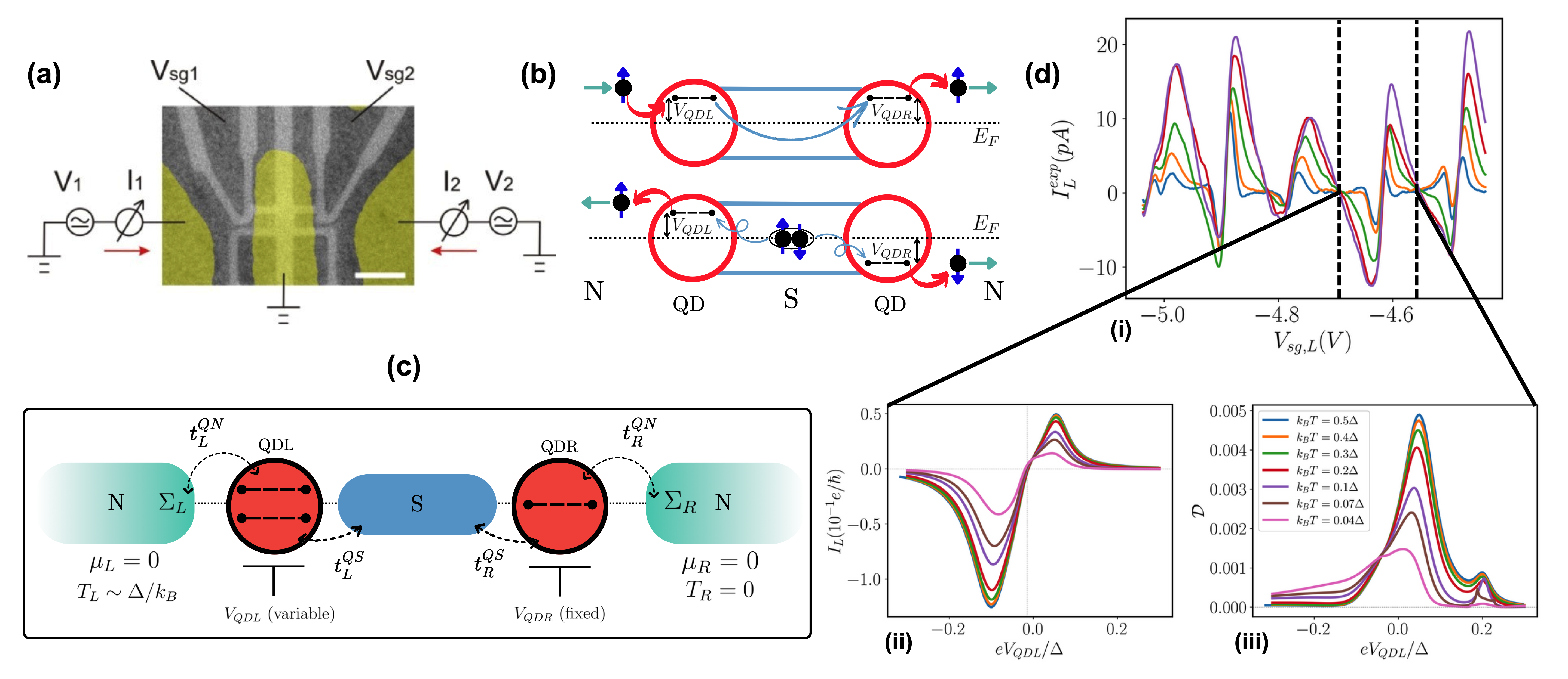
Figure 1: Preliminaries, setup and discussions. (a) False colour image of the QD-CPS hybrid device shown to exhibit non-local currents under a thermoelectric bias [19], with the heater situated on the left side (not shown here). (b) A schematic of the ECT (top) and CAR (bottom) mechanisms in the case of un-hybridized QDs, with ECT dominating at the $(E,E)$ resonance and CAR dominating at the $(E,-E)$ resonance. (c) A detailed schematic of the NEGF-based theoretical model used in this paper consisting of a QD-SC-QD Hamiltonian perturbed by two normal contacts, with QD-N coupling denoted $t^{QN}_{L/R}$ and QD-S coupling denoted $t^{QS}_{L/R}$. The left contact is placed under a thermal bias of order $k_{B}T\sim\Delta$, and there is no voltage bias. The left-dot voltage is varied for analysis. (d) Analyzing currents through the device as a function of thermal bias. Panel (i) shows the experimental local TE current sweep through the QDL as a function of the left gate bias revealing a series of bi-lobe (sawtooth like) current structures and panel (ii) shows a zoomed-in view of a single current bi-lobe structure from our theoretical calculations. Panel (iii) shows the quantum discord computed as a function of $V_{QDL}$.

Coupling a superconducting (SC) region with quantum dots (QD) at its ends permits the spectral engineering of the sub-gap processes, in which the well-spaced and unbroadened QD levels can be made to act as precise probes via electrostatic gating. In addition to the local and CAR processes, the adversarial elastic co-tunneling (ECT) process competes [31]. In particular, a thermoelectric setup eliminates local Andreev processes [32] which are generally orders of magnitude larger than non-local processes that contribute to the CPS signal. In this paper, we theoretically advance the interpretation of the thermoelectric CPS experiment [19], by not only giving a detailed explanation of the observed transport signal, but also by providing new means toward establishing the non-locality of the obtained CPS transport signal.
Using the experimental setup [19] depicted in Fig. 1(a) as our prototype, we develop a quantum transport analysis employing the the Keldysh non-equilibrium Green’s function (NEGF) approach. Focusing on the local thermoelectric (TE) signal noted in the experiment, we establish unambiguously the presence of non-local correlations arising at the Cooper pair splitting resonance. Setting up the NEGF approach for the CPS with minimal assumptions, we resolve the currents into the ECT and CAR components, provide vital insights into the spectral structure of the currents and the QD-SC density of states (DOS). We also compute the quantum discord [33, 34] between the spatially separated QDs to thereby enable us to pin-point the occurrence of non-local correlations that are only CAR induced.
Prior theoretical approaches analyzing CPS have been based either on semi-classical rate equations [35, 36], quantum master equations [37, 38, 39, 40, 41, 42], or using transmission formalism across the individual segments [39, 19] of the device. The master equation approaches are, no doubt, pertinent since the QDs are typically in the Coulomb blockade (CB) regime, such that the charging effects are accounted for within the Fock-space [43] of the sub-system. However, in such approaches, the processes of CAR and ECT are accounted for by describing the SC region via effective coupling parameters. Furthermore, in the current experiment [19], we will see that the discreteness of the energy levels and the effects of the hybridization between the quantum dots, the SC regions and the contacts along with the resulting energy level broadening will be required to provide a detailed interpretation.
Our approach enables a comprehensive insight into the physics of the device without the need for taking into account the superconducting segment as an effective coupling [37, 38] between the QDs. We elucidate the mechanisms of CAR and ECT, outline the effects of quantum broadening and hybridization, and establish the presence of non-local correlations arising at the CPS resonance via the formalism of quantum discord. This results in a general set of guidelines for the gate voltage control of entanglement generation.

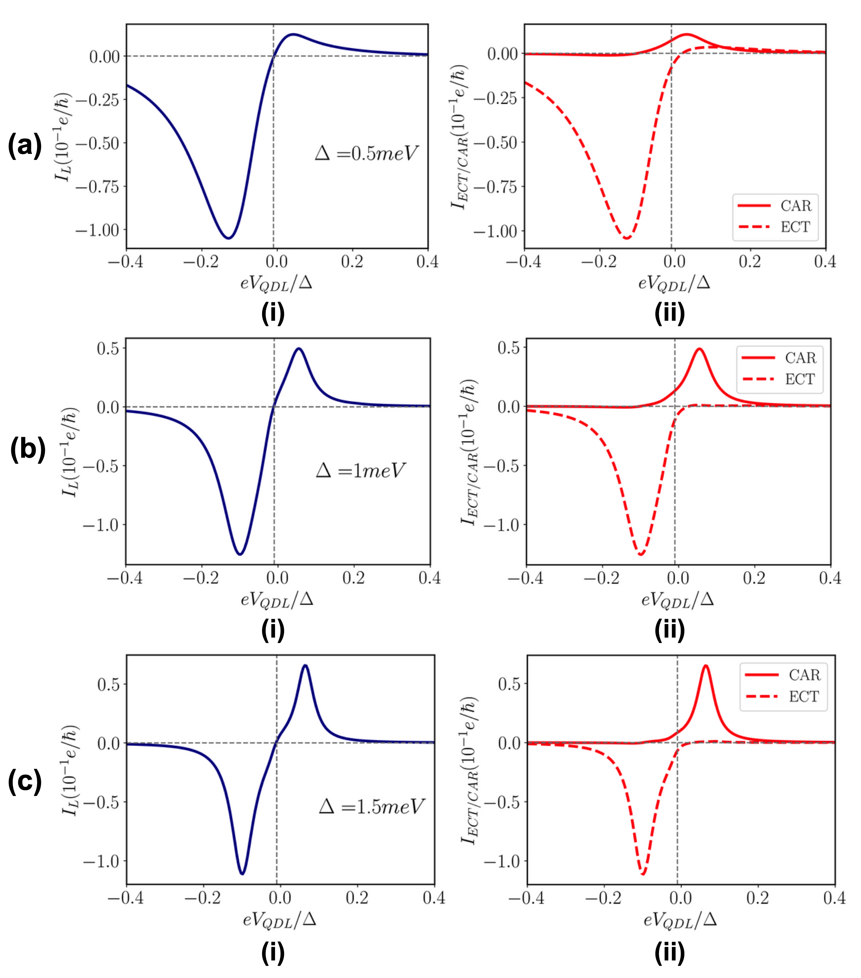
Figure 2: Deconstructing the bi-lobe structure of the local TE currents. Current profiles across the device structure for (a) $\Delta=0.5meV$, (b) $\Delta=1meV$ and (c) $\Delta=1.5meV$. (i) Total current through the left contact ($I_{L}$). (ii) The CAR and ECT resolved currents. All the curves involve varying the left dot voltage $V_{QDL}$ with a fixed right dot voltage of $eV_{QDR}=-0.1\Delta$ and a thermal bias of $k_{B}\Delta T=0.5\Delta$. The chemical potential $\mu=25meV$, and couplings $t^{QN}=t^{QS}=0.02t_{0}$ are held constant as $\Delta$ is varied.

II Formalism

A schematic of the setup is shown in Fig. 1(b,c). The channel region consists of a 1D-superconductor sandwiched between two quantum dots, QDL and QDR. This channel region is tunnel coupled to two normal contacts (N) on the left and right sides. The overall setup Hamiltonian is $H=H_{N}+H_{Ch}+\sum_{\alpha}H_{QD\alpha-N}$, where $H_{Ch},H_{N}$, and $H_{QD\alpha-N}$ (with $\alpha=L,R$), represent the channel Hamiltonian, the Hamiltonian of N contacts and the coupling Hamiltonians between the N region and QDL and the N region and the QDR, respectively.
The Hamiltonian of the channel reads, $H_{Ch}=H_{S}+H_{QDL}+H_{QDR}+H_{QDL,S}+H_{QDR,S}$, where $H_{S}$ is the effective 1D- SC Hamiltonian

$$\begin{aligned} H_{S}&=\sum_{i,\sigma=\uparrow\downarrow}(2t_{S}-\mu_{S})c_{i\sigma}^{\dagger}c_{i\sigma}+\sum_{i,\sigma=\uparrow\downarrow}(t_{S}c_{i+1\sigma}^{\dagger}c_{i\sigma}+h.c.)\\ &+\sum_{i}(\Delta c_{i\uparrow}^{\dagger}c_{i\downarrow}^{\dagger}+h.c.),\end{aligned}$$ (1)

where $t_{S}$ is the hopping parameter within the tight binding model of the 1D-superconductor (see Appendix), $\Delta$ is the superconducting pairing potential, $\mu$ is the electrochemical potential and $h.c.$ is the hermitian conjugate. The summation runs over the site (spin) index $i(\sigma)$. The other components of the channel Hamiltonian, i.e., $H_{QDL}+H_{QDR}+H_{QDL,S}+H_{QDR,S}$ represent the Hamiltonians of the QDL, QDR, the coupling between the QDL, QDR with the SC region. These quantities are defined in detailed in Appendix A.
We denote the energy levels of the left (right) QD by $\{\epsilon_{L(R)}\}$, whose positions are varied via the potentials applied at the local gate electrodes. In accordance with the experiment [19], we do not take into account the Coulomb repulsion on the dots, given that there is no clear evidence of Coulomb blockade or a local double occupancy in the quantum dots. A gate voltage $V_{QDL(R)}$ is applied to the left(right) QD to shift the local energy levels, $\{\epsilon_{L(R)}-eV_{QDL(R)}\}$, where $e$ is the magnitude of the electronic charge. The QDs are coupled with the nearest neighbour SC sites via spin-conserving coupling strengths $t^{QS}_{L(R)}$, which accounts for the hybridization.
For the N contacts, we consider two semi-infinite normal metallic leads in the site basis (See Appendix A) which are coupled with strengths $t^{QN}_{L(R)}$ to the left and right QDs respectively. The semi-infinite structure of the leads is accounted for by the self-energies $\Sigma_{L(R)}$ in the NEGF formalism [44] (see Appendix A). We represent all relevant quantities in the site (spin) Nambu representation $\hat{\psi}_{i}^{\dagger}=\begin{pmatrix}c_{i\uparrow}^{\dagger}&c_{i\downarrow}\end{pmatrix}$, where elements of any matrix at a given site are in the $2\times 2$ electron-hole Nambu space.
In the sub-gap transport regime, one then evaluates the transmissions for the ECT and the CAR processes, as given by

$$T_{ECT}={\rm Tr}\left(\Gamma_{L}^{ee(hh)}G^{r}\Gamma_{R}^{ee(hh)}G^{a}\right)$$ (2)

$$T_{CAR}={\rm Tr}\left(\Gamma_{L}^{ee(hh)}G^{r}\Gamma_{R}^{hh(ee)}G^{a}\right),$$

where, $G^{r}~{}(G^{a})$ is the retarded (advanced) Green’s function, $\Gamma_{L(R)}$ is the broadening matrix associated with the left (right) contact with the superscripts $ee(hh)$ denoting the electron(hole) sub-sectors in the Nambu representation. The net current at the contacts is a sum of these transmissions weighed appropriately with the Fermi-function differences at the contacts [44]. This enables a detailed analysis of the double-lobed TE current signal and understand its resolution into the CAR and ECT components.
Additionally, to establish the non-locality of the quantum correlations between the spatially separated left- and right-QDs, we employ the formalism of quantum discord [34]. The NEGF equations [44, 45, 46] are first solved to get the steady-state behaviour of the system at individual energies $E$, and then a steady-state correlation matrix is computed by integrating electron density lesser Green’s function $G^{n}(E)=-iG^{<}(E)$ (see the Appendix for details) along the energy axis, such that $-i\langle\hat{\psi}_{i}^{\dagger}\hat{\psi}_{j}\rangle=\frac{1}{2\pi}\int dE[G^{n}(E)]_{i,j}$. This is a $2\times 2$ correlator matrix in the Nambu representation with the off-diagonal terms representing the superconducting pairing amplitude. Subsequently, the two-mode occupation-basis density matrix for the up-spin mode of the left QD and the down-spin mode of the right QD is computed using the above steady-state correlation matrix (see Appendix). Quantum discord, defined as the difference between the quantum and classical mutual information, is an indicator of quantum correlations between two systems. Following [33], we compute the two-orbital fermionic discord between the up-spin orbital of the QDL and the down-spin orbital of the QDR to probe correlations in the CPS (see Appendix).

III Results

We start by noting the experimental trace of the local TE current depicted in Fig. 1(d)(i), which comprises a series of double lobes, and that each double-lobe corresponds to a crossing pair of levels between QDL and QDR. Hereon, we focus on the single lobe in order to extract essential physics related to the CPS operation. For this, we include only a single level on both QDs. The right QD level is kept fixed at resonance with the chemical potential, similar to the setup in Fig. 1(c). Figure 1(d)(ii) shows the theoretically calculated left lead current which portrays a single saw-tooth behaviour and temperature variation consistent with the experimental curves. To identify and verify CAR-dominated parameter regimes, we calculate the quantum discord between the left and right dots as shown in Fig. 1(d)(iii). Unlike the TE current signal, the discord peaks only at gate voltages coinciding with one of the lobes. As we will see further, this lobe coinciding with the peak in the discord actually represents CAR contributions to the total current, while the ECT dominates the current in the other lobe. The discord thus confirms the presence of a spin-singlet-correlation between the two dots in the CAR dominated regions and also showcases the absence of such correlations in ECT dominated regimes.
It must be noted however, that, while there could be non-zero mutual information between the $\sigma-\sigma$ orbitals of the QDL-QDR, it does not represent any particle entanglement as it corresponds to correlations of the type $\langle c^{\dagger}_{QDL}c_{QDR}\rangle$. On the other hand, the discord computed here corresponds to the correlations of the form $\langle c^{\dagger}_{QDL}c^{\dagger}_{QDR}\rangle$.

III.1 Resolving CAR and ECT components

To analyze the effects of various parameters on the Cooper pair splitting process, it is necessary to first resolve the TE current signal into its CAR and ECT components. In Fig. 2(a)(i), we plot the TE current for a setup with the SC gap $\Delta=1meV$, chemical potential $\mu=25meV$, a fixed right dot gate voltage $eV_{QDR}=-0.1\Delta$, thermal bias $k_{B}T=0.5\Delta$ and $t^{QN}=t^{QS}=0.02t_{0}$, where $t_{0}={\hbar^{2}}/{(2m^{*}a^{2})}$ for a lattice discretisation of $a=5nm$ evaluates to $t_{0}=184meV$. In Fig. 2(a)(ii), We decompose the current into its CAR (solid) and ECT (dashed) components.
These contributions are discernible through the energetics of the underlying sub-gap transport mechanism. Moving right-to-left along the $V_{QDL}$ axis, when $eV_{QDL}\sim-0.1\Delta$, the left dot level is effectively at $\epsilon_{L}-eV_{QDL}=0.1\Delta$ and resonates with the right dot level positioned at $\epsilon_{R}-eV_{QDR}=0.1\Delta$, thereby leading to a maximum of the ECT process which is essentially just a direct tunneling process mediated through the suppressed sub-gap DOS within the SC region. Next, when $eV_{QDL}\sim 0.1\Delta$ the left dot level is effectively at $\epsilon_{L}-eV_{QDL}=-0.1\Delta$ and satisfies $\epsilon_{L}-eV_{QDL}=-(\epsilon_{R}-eV_{QDR})=0.1$, at which point the CPS process is assisted with a ready availability of energy levels at $E$ and $-E$, leading to a peak in the CAR process.

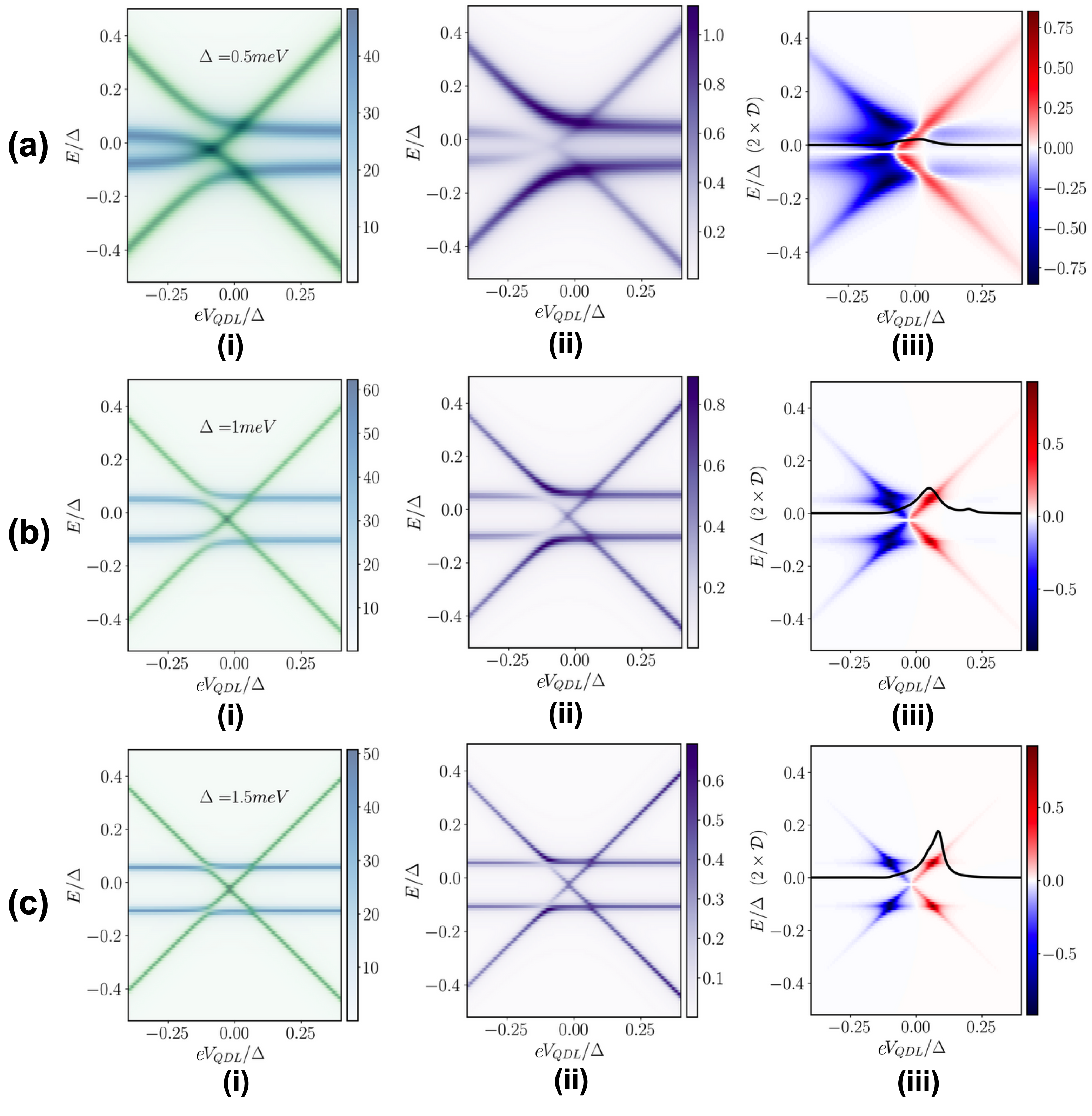
Figure 3: Avoided crossings and the spectral distribution of the CPS currents. For (a) $\Delta=0.5meV$, (b) $\Delta=1meV$ and (c) $\Delta=1.5meV$. (i) Superimposed LDOS of QDL (green) and QDR (blue), with the scalebar representing the same maximum intensity. (ii) The DOS of the mediatingSC segment. (iii) Energy resolved current spectrum $I_{L}(E)$, with the inset curve showing twice the quantum discord $\mathcal{D}$. Parameters are the same as that of Fig.2. All DOS plots are in the units of $\frac{1}{\Delta}$ and current spectra in units of $\frac{e}{\hbar\Delta}$.

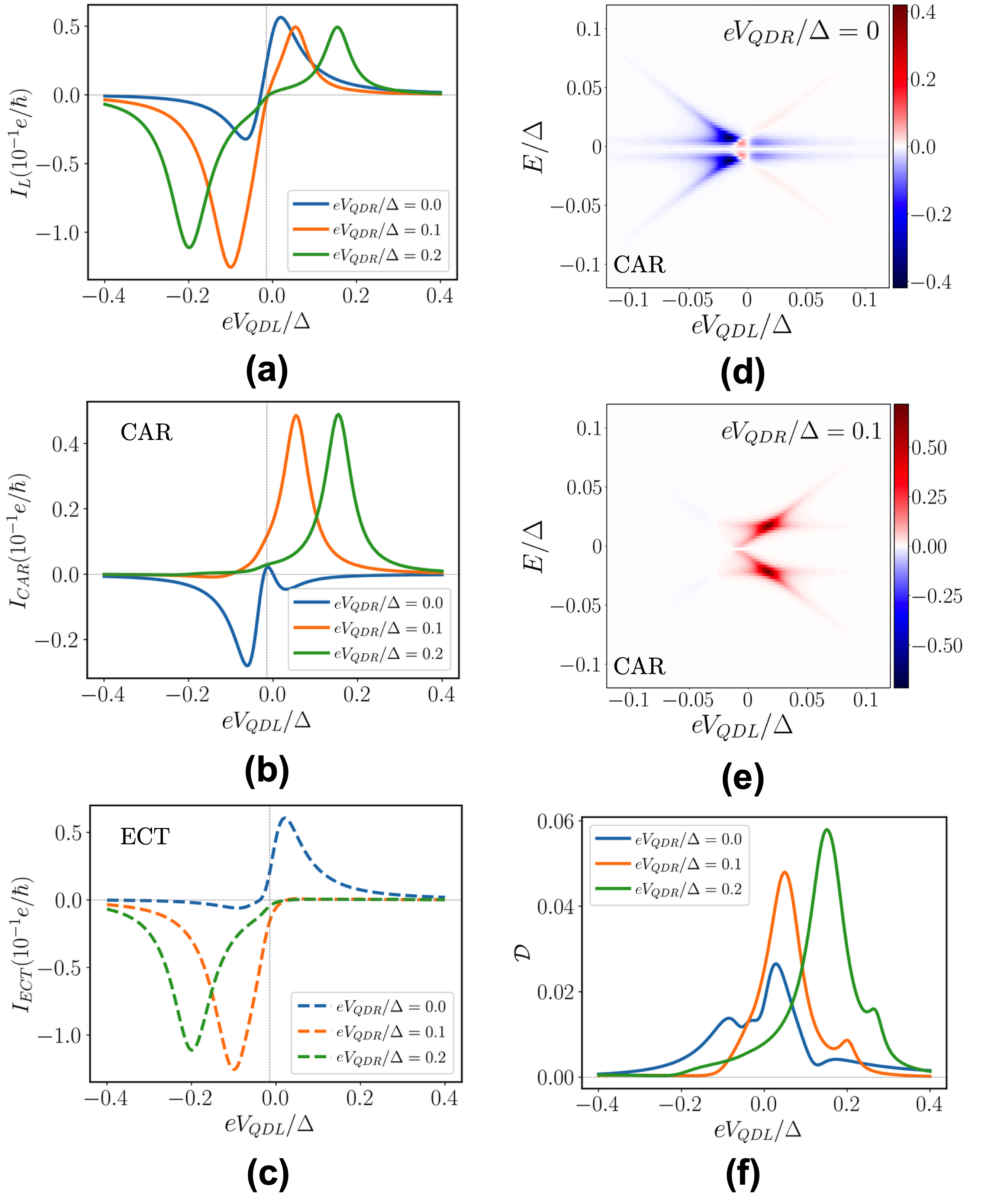
Figure 4: Effect of detuning the QDR. (a) TE current through the left lead $I_{L}$ in units of $0.1e/\hbar$. (b-c) Resolved CAR and ECT currents. (d-e) Energy resolved CAR current for $eV_{QDR}=0.0\Delta$ and $eV_{QDR}=0.1\Delta$ respectively. (f) Quantum discord for $V_{QDR}$ values corresponding to (a). A comparison between the CAR current spectrum in (d) and (e) clearly shows the flipping of the CAR and ECT lobes with respect to $V_{QDL}$ when $V_{QDR}=0\Delta$. This is a non-trivial aspect of level broadening due to hybridization of the QD level.

Including the finite SC segment as an integral part of the analysis, rather than adding effective tunnel coupling between the QDs, as done in master equation approaches [37], brings to fore many nuances. To further elucidate this, in Fig. 2(a-c), we plot the TE current at the left contact for $\Delta=0.5,1.0,\text{ and }1.5meV$ respectively. Looking at Fig. 1(b), for a given placement of $V_{QDR}$, one would expect that the ECT resonances will occur at $E=eV_{QDR}$ and the CAR resonance at $E=-eV_{QDR}$. This is because the ECT resonance occurs due to spin-conserving tunelling process, that takes place when the up (down) -spin electron (hole) levels align. The CAR resonance occurs at just the opposite energetic condition. We thereby note two important subtleties, one, the resonance conditions for the CAR and ECT lobes are not exact. Second, Figs. 2(a)(i), (b)(i) and (c)(i), show that as we increase the order parameter, the CAR component increases, with the ECT component remaining nearly unaltered. Understanding the aforesaid subtleties entail digging deeper into the aspects of level broadening and hybridization which we will discuss now.

III.2 Current spectral decomposition

In the analysis to follow, for our choice of $V_{QDR}=-0.1\Delta$, the ECT (CAR) resonances occur to the left (right) abscissa axis. We observe in Fig. 2 that the ECT curves are asymmetrically distributed about their resonance, whereas the CAR plots are symmetric. Further, we note that as the SC is made stronger from Fig. 2(a)(ii) to Fig. 2(c)(ii), the asymmetry in the ECT curves is less pronounced. This, we will show, is in fact due to the avoided crossings of the ECT process as $\Delta$ is varied.
We illustrate this in Fig. 3, where we show (i) the local DOS (LDOS) at the QDs, (ii) the total DOS inside the SC region and (iii) the energy resolved current with discord superimposed. All DOS plots are in the units of $\frac{1}{\Delta}$ and current spectra in units of $\frac{e}{\hbar\Delta}$. The results are shown for the same set of superconducting strengths as in Fig. 2. As we move from (a) to (c), the $\Delta$ increases, the influence of the QDs on the SC segment is minimal, which manifests as a sharper DOS with decreased broadening.
The QDL LDOS (green, cross-like) is superposed with the QDR LDOS (blue, horizontal line-like) in Fig. 3(a-c)(i), which shows avoided crossings at both the ECT and CAR points. The avoided crossing represents the states of the QD levels in the presence of the SC, with a larger level repulsion when $\Delta$ becomes weaker, indicating a considerable mixing of SC and QD states. This typically happens when the coherence length is large (smaller pairing). Also, such avoided crossings are a generic signature of CAR and ECT processes in a QD-SC-QD setup [37] due to two-level atom like transitions between the empty and the singlet states of the two QDs (see Appendix for further discussion). While the CAR crossing behaves exactly as pointed out in an earlier work [37], the ECT crossing shows non-trivial behaviour as the $\Delta$ becomes stronger, as a direct consequence of contact induced level broadening.
First, we make note that the CAR anticrossings are far less discernible than the ones related to the ECT processes. When we peek into the SC-DOS shown in Fig. 3(iii) column, for the CAR process, we note an equal increase in the QDL and the QDR branches of the SC-DOS. With increasing $\Delta$, the SC segment becomes less influenced by the QD and the CAR magnitude increases with the resonant peak becoming stronger, as noted previously in Fig. 2. This can be clearly seen with the increased contrast of the CAR spectrum as $\Delta$ increases, and is also reflected in the quantum discord.
As mentioned earlier, the CAR current magnitude increases [47], while the ECT remains largely the same. While the thermoelectric bias depends on $\Delta$, this only affects the currents weakly. Looking carefully at the CAR resonances for the current spectrum along the column Fig.3(iii), we notice specifically from Fig.3(c) (iii) that there is a current back flow contribution as noted from the blue striped region. This clearly corresponds to processes that involve mixing of the QD levels with those of the SC, thereby promoting normal reflections in addition to the Andreev processes. This leads to the weakening the CAR leading to a smaller TE current. The CAR processes get stronger with sharper spectral resolution as the $\Delta$ is increased, leading to an increase in the total current, which is an integral over the energy axis at a given $V_{QDL}$.

III.3 Detuning the QDR

Moving further, we analyze the effects of detuning the right dot with respect to the electrochemical potential (kept at zero) of the system. Figure 4(a) demonstrates the TE current through the left lead $I_{L}$ as a function of left dot gate voltage $V_{QDL}$ for $eV_{QDR}\in\{0.0,0.1,0.2\}\Delta$. The characteristic saw-tooth widens upon increasing $V_{QDR}$. Upon resolving the left lead current in Fig. 4(b) and (c), it is clear that the CAR and ECT peaks of the the current move away from the resonance point of the hybridised dot level. Upon further inspection of the resolved CAR and ECT currents, we note that for the case of zero detuning, the peaks of CAR and ECT are interchanged, accompanied by a parity crossing in the currents.
The parity crossing observed in the currents is characteristic to a TE bias when only a temperature gradient applied. The electron and hole currents flip when the chemical potential falls precisely at the mid-gap of a given spectrum. In our case, due to the finite hybridization between either dot and the SC region, this does not happen at the apparent mid-gap symmetry point, which is $eV_{QDR}=0$. This can be further elucidated in Fig. 4(d-e), where we plot the energy resolved spectrum of the CAR currents for (d) $eV_{QDR}/\Delta=0$ and (e) $eV_{QDR}/\Delta=0.1$.
In Fig. 4(d), we note two parity changes upon moving from left to right along the $V_{QDL}$ axis and a positive CAR peak on the left side, which moves over to the right side with a single parity crossing upon increasing the detuning to $0.1\Delta$ as in Fig. 4(e). Thus, there exists a critical detuning magnitude that is dependent on theSC region and the coupling strengths, after which, the expected behaviour sets in for the CAR and ECT peaks. This interchange of the CAR and ECT lobes is crucial to understand when interpreting the experimental current traces.
Lastly, Fig. 4(f) shows the discord for corresponding $V_{QDR}$ values. While the discord peak moves with the CAR maxima, a critical difference is noted between the $eV_{QDR}/\Delta=0$ and the $eV_{QDR}/\Delta\in\{0.1,0.2\}$ cases, with the location of the side-peak moving from the left to the right respectively, thereby emphasizing the physics of hybridization due to the contact broadening.

IV Discussions and Inferences

We conducted a detailed analysis of the observed local TE currents [19], which revealed crucial insights into the operating regimes and the complex nature of the correlations. The behaviors of the CAR and ECT anticrossings at different gate voltages highlighted the significant roles of hybridization with the SC segment and level broadening. A detailed current spectral analysis connected these features to the observed transport signals, examining parity reversal and the shifted resonances of the CAR processes. Finally, we established the presence of non-local correlations in the CAR current signal, linking them to quantum discord. Our analysis provides crucial insights into how gate voltage controls entanglement generation in superconducting-hybrid Cooper pair splitters. An interesting future direction involves integrating the full spectral information available via our calculations into a time-dependent quantum master equation [48] to improve upon recently proposed driving protocols for maximizing CPS efficiency [37, 38]. Realizing CPS in two-dimensional topological materials is yet another promising direction [49, 46]. Additionally, it remains to be seen whether the mechanism of spin-valley locking in certain systems, for example, bilayer graphene or transition-metal dichalcogenide quantum dots, might be used to engineer more precise control over the splitting process in such devices, as well as harness non-local valley entanglement.

Appendix A Setup and Formalism

A schematic of our setup is shown in Fig. 1(c) of the main text. The device consists of a superconducting (SC) region sandwiched between two quantum dots (QD). The QDs are tunnel coupled to two normal contacts (N) on the left and right. The length of theSC region is smaller than the SC coherence length to ensure that non-local sub-gap processes like ECT and CAR can manifest with considerable magnitude. Each QD may have multiple levels with level positions and separations independent of each other. We denote the levels of the left(right) QD by $\{\epsilon_{L(R)}\}$. A gate voltage $V_{QDL(R)}$ can be applied to the left(right) QD to control its local chemical potential and shift the levels to $\{\epsilon_{L(R)}-eV_{QDL(R)}\}$, where $e$ is the electronic charge. The Hamiltonian of the QD-SC-QD region is given by

$$H =H_{S}+H_{QDL}+H_{QDR}+H_{QDL-S}+H_{QDR-S}$$ (3)

where, $H_{S}$ is the Hamiltonian of theSC region

$$\begin{aligned} H_{S}&=\sum_{i=1}^{N_{s}}\sum_{\sigma=\uparrow\downarrow}(2t_{S}-\mu_{S})c_{i\sigma}^{\dagger}c_{i\sigma}-\sum_{i=1}^{N_{s}-1}\sum_{\sigma=\uparrow\downarrow}t_{0}c_{i+1\sigma}^{\dagger}c_{i\sigma}\\ &+\sum_{i=1}^{N_{s}}\Delta c_{i\uparrow}^{\dagger}c_{i\downarrow}^{\dagger}+h.c.\end{aligned}$$ (4)

$N_{s}$ is the number of sites in the SC region, $c_{i\sigma}^{(\dagger)}$ are the annihilation(creation) operators at site $i$, $\mu_{S}$ is the chemical potential, $\Delta$ is the SC gap parameter and $t_{S}=\frac{\hbar^{2}}{2m^{*}a^{2}}$ is the tight-binding hopping parameter with electron reduced mass $m^{*}$ and lattice spacing $a$. The Hamiltonians of the left(right) dot read,

$$H_{QDL(R)}=\sum_{i=1,\sigma=\uparrow\downarrow}^{N_{dL(R)}}(\epsilon_{L(R)}-eV_{QDL(R)})d_{i\sigma L(R)}^{\dagger}d_{i\sigma L(R)}$$ (5)

$N_{dL(R)}$ are the number of levels in the left(right) dot, operators $d_{i\sigma}^{(\dagger)}$ annihilate(create) electrons in a state $i$ with spin $\sigma$ in the respective dot and $\epsilon_{L(R)}$ and $eV_{QDL(R)}$ define the energy levels of the dot.
Further, we have $H_{QDL(R)-S}$, which is the Hamiltonian that couples either dot to theSC region,

$$H_{QDL(R)-S}=\sum_{i=1,\sigma=\uparrow\downarrow}^{N_{dL(R)}}(t^{QS}_{L(R)}d_{i\sigma L(R)}^{\dagger}c_{1(N_{S})\sigma}+h.c.)$$ (6)

here, $t^{QS}_{L(R)}$ denotes the hopping between the left(right) QD and the SC. For the contacts, we consider two semi-infinite metallic leads in the eigenbasis with the Hamiltonian defined as

$$H_{N} =\sum_{i,\sigma=\uparrow\downarrow}(2t_{N}-\mu_{N})b_{i\sigma}^{\dagger}b_{i\sigma}-\sum_{i,\sigma=\uparrow\downarrow}t_{N}b_{i+1\sigma}^{\dagger}b_{i\sigma}+h.c.$$ (7)

where, $b_{i\sigma}^{(\dagger)}$ are the annihilation(creation) operators in the contacts, $\mu_{N}$ is the chemical potential of the leads and $t_{N}$ is the tight-binding hopping parameter. The coupling between the semi-infinite leads and the QD are mediated by a Hamiltonian of the form

$$H_{QDL(R)-N}=\sum_{i=1,\sigma=\uparrow\downarrow}^{N_{dL(R)}}(t^{QN}_{L(R)}d_{i\sigma L(R)}^{\dagger}b_{1\sigma}+h.c.)$$ (8)

here, $t^{QN}_{L(R)}$ denotes the hopping between the left (right) QD and the the left (right) contact, which is in-turn taken into account via the contact self-energies which are calculated iteratively using the surface Green’s function method.

Appendix B Quantum Transport through the QD-S-QD system

For transport calculations we use the Keldysh Green’s formalism cast in terms of the non-equilibrium Green’s functions (NEGF), described in detail herein. Under the NEGF method, the semi-infinite leads and their coupling to the device are accounted through self-energies $\Sigma_{L}(R)$ of the left(right) contact. Given the Hamiltonian of the channel $H_{Ch}$ and the self-energies of the metallic contacts on the left(right) $\Sigma_{L(R)}$ in their matrix representation, the retarded Green’s function matrix at energy $E$ for the QDL-SC-QDR system is calculated as

$$G^{r}(E)=\left((E+i\eta)I-H_{Ch}-\Sigma_{L}-\Sigma_{R}\right)^{-1}$$ (9)

where, $\Sigma_{L(R)}$ are the contact self-energies, $I$ is the identity matrix, and $\eta>0$ is a small damping parameter. In the sub-gap transport regime, transmission manifests in three distinct processes – Andreev transmission ($T_{A}$), elastic co-tunneling ($T_{ECT}$) and crossed-Andreev transmission ($T_{CAR}$), given by

$$T_{A}={\rm Tr}\left(\Gamma_{L}^{ee(hh)}G^{r}\Gamma_{L}^{hh(ee)}G^{a}\right)$$ (10)

$$T_{ECT}={\rm Tr}\left(\Gamma_{L}^{ee(hh)}G^{r}\Gamma_{R}^{ee(hh)}G^{a}\right)$$

$$T_{CAR}={\rm Tr}\left(\Gamma_{L}^{ee(hh)}G^{r}\Gamma_{R}^{hh(ee)}G^{a}\right)$$

where, $G^{a}=(G^{r})^{\dagger}$ is the advanced Greens function, $\Gamma_{L(R)}=i[\Sigma_{L(R)}-\Sigma_{L(R)}^{\dagger}]$ are the broadening matrices and $\Gamma_{L(R)}^{ee(hh)}$ are the electron(hole) sub-sectors of $\Gamma_{L(R)}$. The energy resolved current at the left-lead can be calculated as

$$I_{L}(E) =T_{A}(E)[f_{L}^{e}(E)-f_{L}^{h}(E)]$$ (11)

$$+T_{ECT}(E)[f_{L}^{e}(E)-f_{R}^{e}(E)]$$

$$+T_{CAR}(E)[f_{L}^{e}(E)-f_{R}^{h}(E)]$$

where, $f_{L(R)}^{e/h}(E)=f(E\pm eV_{L(R),T_{L(R)}})$ ($\pm$ corresponding to $e/h$) and $f(E,T)$ is the Fermi-Dirac distribution at energy $E$ and at temperature $T$. The net current at the left contact can now be computed as,

$$I_{L}=\int_{-\infty}^{\infty}I_{L}(E)dE$$ (12)

Appendix C Correlations and QDL-QDR density matrix

Given the broadening matrices $\Gamma_{L(R)}$, one can further compute the in-scattering functions as,

$$\Sigma^{in}_{L(R)}(E)=f(E,V_{L(R)},T_{L(R)})\cdot\Gamma_{L(R)}.$$ (13)

Coupling this with the previously calculated Green’s functions, we get the correlation matrix $G^{n}$ as,

$$G^{n}(E)=G^{r}\Sigma^{in}G^{a}$$ (14)

where $\Sigma^{in}=\Sigma^{in}_{L}+\Sigma^{in}_{R}$ is the net in-scattering function. This matrix encodes the quadratic correlators at an energy $E$,

$$[G^{n}(E)]_{ij\alpha\beta}\sim\langle c^{(\dagger})_{i\alpha}c^{(\dagger})_{j\beta}\rangle(E).$$ (15)

The aforesaid Green’s function encodes the non-equilibrium correlators, which in the original parlance is related to the lesser Green’s function $G^{n}(E)=-iG^{<}(E)$, in the steady-state of the system perturbed by the contacts. Given this, we compute the correlation matrix by integrating along the energy space as follows,

$$[\langle c^{(\dagger})_{i\alpha}c^{(\dagger})_{j\beta}\rangle]_{ij\alpha\beta}=\frac{1}{2\pi}\int[G^{n}(E)]dE.$$ (16)

With this, we can obtain the specific correlation matrix in the QDL-QDR subspace. We further proceed by obtaining the two-mode density matrices in the $\{\ket{0},\ket{1}\}\otimes\{\ket{0},\ket{1}\}$ occupation basis for the up (down) -spin mode on the QDL and the down (up)-spin mode on the QDR. We recap the general procedure for calculating the density matrix and subsequently the two-mode discord, as outlined in [33].
Given the correlation matrix $[\langle c^{(\dagger})_{i}c^{(\dagger})_{j}\rangle]_{ij}$ of a two-mode system, we compute the density matrix in the
$\left\{c_{i}^{\dagger}c_{j}^{\dagger}|0\rangle,c_{i}^{\dagger}|0\rangle,c_{j}^{\dagger}|0\rangle,|0\rangle\right\}$ as [50],

$$\rho_{ij}=\left(\begin{array}[]{cccc}\langle c_{i}^{\dagger}c_{i}c_{j}^{\dagger}c_{j}\rangle&0&0&\langle c_{j}c_{i}\rangle\\ 0&\langle c_{i}^{\dagger}c_{i}c_{j}c_{j}^{\dagger}\rangle&\langle c_{j}^{\dagger}c_{i}\rangle&0\\ 0&\langle c_{i}^{\dagger}c_{j}\rangle&\langle c_{i}c_{i}^{\dagger}c_{j}^{\dagger}c_{j}\rangle&0\\ \langle c_{i}^{\dagger}c_{j}^{\dagger}\rangle&0&0&\langle c_{i}c_{i}^{\dagger}c_{j}c_{j}^{\dagger}\rangle\end{array}\right).$$

The quantum discord is defined as the difference between two measures of information shared between systems $A$ and $B$. Given the classical mutual information $I(A:B)$ and the quantum mutual information $S(A:B)$, we compute the discord $\delta(A:B)$ as

$$\delta(A:B):=S(A:B)-I(A:B),$$ (17)

where the quantum mutual information is given as

$$S(A:B)=S(A)+S(B)-S(A,B),$$ (18)

where $S(A/B)$ are the von Neumann entropies of the $A/B$ subsystems, and $S(A,B)$ is the joint entropy of the $AB$ system. Further, the optimized classical mutual information is defined as,

$$I(A:B)=\max_{\{\Pi_{k}^{B}\}}S(A)-S(A,B|\{\Pi_{k}^{B}\}),$$ (19)

where, $\Pi_{k}^{B}$ is a measurement onto the B subsystem, which is optimized to learn the maximal information about the A subsystem. Formally,

$$S\left(\rho^{(A,B)}\mid\left\{\Pi_{k}^{B}\right\}\right)=\sum_{k}p_{k}S\left(\rho_{k}^{AB}\right),$$

where,

$$\rho_{k}^{(A,B)}=\frac{1}{p_{k}}\Pi_{k}^{B}\rho^{AB}\Pi_{k}^{B}$$

is a possible post-measurement state and

$$p_{k}=\operatorname{tr}\left(\Pi_{k}^{B}\rho^{AB}\Pi_{k}^{B}\right)$$

is the probability of getting the measurement outcome $k$. Now, it was pointed out that the optimization inherent in the computation of quantum discord for fermionic systems is ruled out because of the parity-superselection rule [33]. Ignoring the superselection rule and carrying out the optimization can lead to an over-estimation of the correlations. Thus, the only possible measurements are,

$$\Pi_{0}=c_{j}c_{j}^{\dagger},\quad\Pi_{1}=c_{j}^{\dagger}c_{j},$$

and the only possible post-measurement states are

$$\rho_{0}^{(A,B)} =\frac{1}{\rho_{1}+\rho_{3}}\left(\begin{array}[]{cccc}\rho_{1}&0&0&0\\ 0&0&0&0\\ 0&0&\rho_{3}&0\\ 0&0&0&0\end{array}\right),$$

$$\rho_{1}^{(A,B)} =\frac{1}{\rho_{2}+\rho_{4}}\left(\begin{array}[]{cccc}0&0&0&0\\ 0&\rho_{2}&0&0\\ 0&0&0&0\\ 0&0&0&\rho_{4}.\end{array}\right)$$

Because of this, the conditional entropy can be written as

$$S\left(\rho^{(A,B)}\mid\left\{\Pi_{k}^{(B)}\right\}\right)=S\left(\mathcal{Z}\left(\rho^{(A,B)}\right)\right)-S\left(\rho^{(B)}\right),$$

where $\mathcal{Z}(\rho)$ is the dephasing channel, which destroys the off-diagonal elements of $\rho$. Finally, the quantum discord can be written as

$$\delta(A,B)=S\left(\mathcal{Z}\left(\rho^{(A,B)}\right)\right)-S\left(\rho^{(A,B)}\right).$$

Appendix D CAR and ECT avoided crossings

The SC region in a QD-S-QD setup can be thought of as a bridge that mediates interaction between the two QDs. In the case with single-level QDs, the coupling between the dots can be considered as a perturbation to the double quantum dot (DQD) system and can be integrated out to yield an effective Hamiltonian [51, 52]. The Fock space of the DQD system is spanned by 16 states, of which the doublet states are discarded as a large Coulomb blockade in the dots restricts double occupancy. The remaining states are the unoccupied states $|0;0\rangle=|0\rangle$, four singly-occupied states $|\sigma;0\rangle=|L\sigma\rangle$ and $|0;\sigma\rangle=|R\sigma\rangle$ with $\sigma=\uparrow\text{or}\downarrow$, a singlet state $|S\rangle=\frac{1}{\sqrt{2}}(|\uparrow;\downarrow\rangle-|\downarrow;\uparrow\rangle)$ and three triplet states $|\uparrow;\uparrow\rangle$, $|\downarrow;\downarrow\rangle$, $\frac{1}{\sqrt{2}}(|\uparrow;\downarrow\rangle+|\downarrow;\uparrow\rangle)$. The triplet states are ignored from the effective Fock space considering the s-wave pairing symmetry of the superconducting interaction and therefore, the effective Hamiltonian for the system is spanned by six states $|0;0\rangle,|\sigma;0\rangle,|0;\sigma\rangle\text{ and }|S\rangle$ with ECT processes coupling the singly occupied states and the CAR processes coupling the unoccupied states and the singlet state [52, 51].
Near the ECT point $\epsilon_{L}=\epsilon_{R}$, and the expectation values $\langle\frac{1}{\sqrt{2}}(d_{L\uparrow}^{\dagger}d_{R\downarrow}^{\dagger}-d_{L\downarrow}^{\dagger}d_{R\uparrow}\rangle=\langle\frac{1}{\sqrt{2}}(d_{R\downarrow}d_{L\uparrow}-d_{R\uparrow}d_{L\downarrow}\rangle=|0\rangle\langle S|=|S\rangle\langle 0|=0$, thereby restricting transitions between the singlet and the unoccupied state. The effective Hamiltonian can then be written as

$$H_{eff}=\sum_{\sigma=\uparrow\downarrow}\epsilon_{L}d_{L\sigma}^{\dagger}d_{L\sigma}+\epsilon_{R}d_{R\sigma}^{\dagger}d_{R\sigma}+\\ \Gamma_{ECT}d_{L\sigma}^{\dagger}d_{R\sigma}+h.c.,$$ (20)

which is a typical two-state system treatment between two uncoupled levels $\{|L\uparrow\rangle,|R\uparrow\rangle\}$ and $\{|L\downarrow\rangle,|R\downarrow\rangle\}$ and therefore manifests as an avoided crossing between the bare states with eigen-energies given by

$$E^{ECT}_{\pm}=\frac{(\epsilon_{L}+\epsilon_{R})}{2}\pm\frac{1}{2}\sqrt{(\epsilon_{L}-\epsilon_{R})^{2}+\Gamma_{ECT}^{2}}.$$ (21)

At the CAR point $\epsilon_{L}=-\epsilon_{R}$, the expectation values $\langle d_{L\sigma}^{\dagger}d_{R\sigma}\rangle=\langle d_{R\sigma}^{\dagger}d_{L\sigma}\rangle=|L\sigma\rangle\langle R\sigma|=|R\sigma\rangle\langle L\sigma|=0$, thereby restricting transitions between the singly-occupied states. The effective Hamiltonian is given by

$$H_{eff}=\sum_{\sigma=\uparrow\downarrow}\epsilon_{L}d_{L\sigma}^{\dagger}d_{L\sigma}+\epsilon_{R}d_{R\sigma}^{\dagger}d_{R\sigma}+\\ \frac{\Gamma_{CAR}}{\sqrt{2}}(d_{L\uparrow}^{\dagger}d_{R\downarrow}^{\dagger}-d_{L\downarrow}^{\dagger}d_{R\uparrow}^{\dagger})+h.c.,$$ (22)

which can be mapped to a typical two-state Hamiltonian as well, with $|0\rangle$ and $|S\rangle$ as the levels and an avoided-crossing denoting the hybridization between the levels. The eigen-energies are given by

$$E^{CAR}_{\pm}=\frac{(\epsilon_{L}-\epsilon_{R})}{2}\pm\frac{1}{2}\sqrt{(\epsilon_{L}+\epsilon_{R})^{2}+\Gamma_{CAR}^{2}}.$$ (23)

At the centre of the two avoided-crossings, the energy difference between the branches is given by $\Gamma_{ECT}$ and $\Gamma_{CAR}$ respectively. From [51, 52] $\Gamma_{ECT}=\frac{\mu}{\mu^{2}+\Delta^{2}}$ and $\Gamma_{CAR}=\frac{\Delta}{\mu^{2}+\Delta^{2}}$. Therefore, the avoided-crossing gap is a decreasing function in the case of ECT and a small-valued increasing function in the case of CAR.

References

- Lesovik et al. [2001] G. B. Lesovik, T. Martin, and G. Blatter, The European Physical Journal B-Condensed Matter and Complex Systems 24, 287 (2001).
- Recher et al. [2001a] P. Recher, E. V. Sukhorukov, and D. Loss, Phys. Rev. B 63, 165314 (2001a).
- Deutscher [2002] G. Deutscher, Journal of superconductivity 15, 43 (2002).
- Herrmann et al. [2010] L. G. Herrmann, F. Portier, P. Roche, A. L. Yeyati, T. Kontos, and C. Strunk, Phys. Rev. Lett. 104, 026801 (2010).
- Schindele et al. [2012] J. Schindele, A. Baumgartner, and C. Schönenberger, Phys. Rev. Lett. 109, 157002 (2012).
- Ranni et al. [2022] A. Ranni, E. T. Mannila, A. Eriksson, D. S. Golubev, J. P. Pekola, and V. F. Maisi, Phys. Rev. Lett. 129, 207703 (2022).
- Ranni et al. [2021] A. Ranni, F. Brange, E. T. Mannila, C. Flindt, and V. F. Maisi, Nature Communications 12, 6358 (2021).
- Das et al. [2012a] A. Das, Y. Ronen, M. Heiblum, D. Mahalu, A. V. Kretinin, and H. Shtrikman, Nature Communications 3, 1165 (2012a).
- Fülöp et al. [2015] G. Fülöp, F. Domínguez, S. d’Hollosy, A. Baumgartner, P. Makk, M. H. Madsen, V. A. Guzenko, J. Nygård, C. Schönenberger, A. Levy Yeyati, and S. Csonka, Phys. Rev. Lett. 115, 227003 (2015).
- Baba et al. [2018] S. Baba, C. Jünger, S. Matsuo, A. Baumgartner, Y. Sato, H. Kamata, K. Li, S. Jeppesen, L. Samuelson, H. Q. Xu, C. Schönenberger, and S. Tarucha, New Journal of Physics 20, 063021 (2018).
- Kürtössy et al. [2022] O. Kürtössy, Z. Scherübl, G. Fülöp, I. E. Lukács, T. Kanne, J. Nygård, P. Makk, and S. Csonka, npj Quantum Materials 7, 88 (2022).
- Wang et al. [2022] G. Wang, T. Dvir, G. P. Mazur, C.-X. Liu, N. van Loo, S. L. D. ten Haaf, A. Bordin, S. Gazibegovic, G. Badawy, E. P. A. M. Bakkers, M. Wimmer, and L. P. Kouwenhoven, Nature 612, 448 (2022).
- Hofstetter et al. [2009] L. Hofstetter, S. Csonka, J. Nygård, and C. Schönenberger, Nature 461, 960 (2009).
- Hofstetter et al. [2011] L. Hofstetter, S. Csonka, A. Baumgartner, G. Fülöp, S. d’Hollosy, J. Nygård, and C. Schönenberger, Phys. Rev. Lett. 107, 136801 (2011).
- de Jong et al. [2023] D. de Jong, C. G. Prosko, L. Han, F. K. Malinowski, Y. Liu, L. P. Kouwenhoven, and W. Pfaff, Phys. Rev. Lett. 131, 157001 (2023).
- Borzenets et al. [2016] I. V. Borzenets, Y. Shimazaki, G. F. Jones, M. F. Craciun, S. Russo, M. Yamamoto, and S. Tarucha, Scientific Reports 6, 23051 (2016).
- Pandey et al. [2021] P. Pandey, R. Danneau, and D. Beckmann, Phys. Rev. Lett. 126, 147701 (2021).
- Tan et al. [2015a] Z. B. Tan, D. Cox, T. Nieminen, P. Lähteenmäki, D. Golubev, G. B. Lesovik, and P. J. Hakonen, Phys. Rev. Lett. 114, 096602 (2015a).
- Tan et al. [2021] Z. B. Tan, A. Laitinen, N. S. Kirsanov, A. Galda, V. M. Vinokur, M. Haque, A. Savin, D. S. Golubev, G. B. Lesovik, and P. J. Hakonen, Nature Communications 12, 138 (2021).
- Kirsanov et al. [2019] N. S. Kirsanov, Z. B. Tan, D. S. Golubev, P. J. Hakonen, and G. B. Lesovik, Phys. Rev. B 99, 115127 (2019).
- Cao et al. [2015] Z. Cao, T.-F. Fang, L. Li, and H.-G. Luo, Applied Physics Letters 107, 212601 (2015), https://pubs.aip.org/aip/apl/article-pdf/doi/10.1063/1.4936380/13465334/212601_1_online.pdf .
- Tan et al. [2015b] Z. B. Tan, D. Cox, T. Nieminen, P. Lähteenmäki, D. Golubev, G. B. Lesovik, and P. J. Hakonen, Phys. Rev. Lett. 114, 096602 (2015b).
- Sánchez et al. [2018] R. Sánchez, P. Burset, and A. L. Yeyati, Phys. Rev. B 98, 241414 (2018).
- Cottet [2012] A. Cottet, Physical Review B 86, 075107 (2012).
- Michałek and Bułka [2021] G. Michałek and B. R. Bułka, New Journal of Physics 23, 023009 (2021), publisher: IOP Publishing.
- Herrmann et al. [2012] L. Herrmann, P. Burset, W. Herrera, F. Portier, P. Roche, C. Strunk, A. L. Yeyati, and T. Kontos, arXiv preprint arXiv:1205.1972 (2012).
- Das et al. [2012b] A. Das, Y. Ronen, M. Heiblum, D. Mahalu, A. V. Kretinin, and H. Shtrikman, Nature communications 3, 1165 (2012b).
- Scherübl et al. [2022] Z. Scherübl, G. m. H. Fülöp, J. Gramich, A. Pályi, C. Schönenberger, J. Nygård, and S. Csonka, Phys. Rev. Res. 4, 023143 (2022).
- Bordoloi et al. [2022] A. Bordoloi, V. Zannier, L. Sorba, C. Schönenberger, and A. Baumgartner, Nature 612, 454 (2022).
- Soller et al. [2013] H. Soller, L. Hofstetter, and D. Reeb, Europhysics Letters 102, 50009 (2013).
- Recher et al. [2001b] P. Recher, E. V. Sukhorukov, and D. Loss, Phys. Rev. B 63, 165314 (2001b).
- Hussein et al. [2019a] R. Hussein, M. Governale, S. Kohler, W. Belzig, F. Giazotto, and A. Braggio, Phys. Rev. B 99, 075429 (2019a).
- Faba et al. [2021] J. Faba, V. Martín, and L. Robledo, Physical Review A 103, 032426 (2021).
- Ollivier and Zurek [2001] H. Ollivier and W. H. Zurek, Physical review letters 88, 017901 (2001).
- Scherübl et al. [2019] Z. Scherübl, A. Pályi, and S. Csonka, Beilstein Journal of Nanotechnology 10, 363 (2019).
- Albert et al. [2011] M. Albert, C. Flindt, and M. Büttiker, Physical review letters 107, 086805 (2011).
- Brange et al. [2024] F. Brange, R. Baruah, and C. Flindt, Physical Review B 109, L081402 (2024).
- Brange et al. [2021a] F. Brange, K. Prech, and C. Flindt, Physical Review Letters 127, 237701 (2021a).
- Hussein et al. [2019b] R. Hussein, M. Governale, S. Kohler, W. Belzig, F. Giazotto, and A. Braggio, Physical Review B 99, 075429 (2019b), arXiv:1806.04569 [cond-mat].
- Sauret et al. [2004] O. Sauret, D. Feinberg, and T. Martin, Phys. Rev. B 70, 245313 (2004).
- Tam et al. [2021] M. Tam, C. Flindt, and F. Brange, Physical Review B 104, 245425 (2021).
- Walldorf et al. [2020] N. Walldorf, F. Brange, C. Padurariu, and C. Flindt, Physical Review B 101, 205422 (2020), publisher: American Physical Society.
- Das et al. [2022] A. Das, A. A. Khan, S. D. Mishra, P. Solanki, B. De, B. Muralidharan, and S. Vinjanampathy, Quantum Science and Technology 7, 045034 (2022).
- Kejriwal and Muralidharan [2022] A. Kejriwal and B. Muralidharan, Phys. Rev. B 105, L161403 (2022).
- Arora et al. [2024] A. Arora, A. Kejriwal, and B. Muralidharan, New Journal of Physics 26, 023038 (2024).
- Midha et al. [2024] S. Midha, K. Jana, and B. Muralidharan, Journal of Physics D: Applied Physics 57, 135308 (2024).
- Falci et al. [2001] G. Falci, D. Feinberg, and F. W. J. Hekking, Europhysics Letters 54, 255 (2001).
- Jin and Li [2022] J. Jin and X.-Q. Li, New Journal of Physics 24, 093009 (2022).
- Sato et al. [2010] K. Sato, D. Loss, and Y. Tserkovnyak, Phys. Rev. Lett. 105, 226401 (2010).
- Di Tullio et al. [2018] M. Di Tullio, N. Gigena, and R. Rossignoli, Physical Review A 97, 062109 (2018).
- Brange et al. [2021b] F. Brange, K. Prech, and C. Flindt, Phys. Rev. Lett. 127, 237701 (2021b).
- Liu et al. [2022] C.-X. Liu, G. Wang, T. Dvir, and M. Wimmer, Phys. Rev. Lett. 129, 267701 (2022).