MATES: Model-Aware Data Selection for Efficient Pretraining with Data Influence Models

Abstract

Pretraining data selection has the potential to improve language model pretraining efficiency by utilizing higher-quality data from massive web data corpora. Current data selection methods, which rely on either hand-crafted rules or larger reference models, are conducted statically and do not capture the evolving data preferences during pretraining. In this paper, we introduce model-aware data selection with data influence models (MATES), where a data influence model continuously adapts to the evolving data preferences of the pretraining model and then selects the data most effective for the current pretraining progress. Specifically, we fine-tune a small data influence model to approximate oracle data preference signals collected by locally probing the pretraining model and to select data accordingly for the next pretraining stage. Experiments on Pythia and the C4 dataset demonstrate that MATES significantly outperforms random data selection on extensive downstream tasks in both zero- and few-shot settings. It doubles the gains achieved by recent data selection approaches that leverage larger reference models and reduces the total FLOPs required to reach certain performances by half. Further analysis validates the ever-changing data preferences of pretraining models and the effectiveness of our data influence models to capture them. Our code is open-sourced at this URL.

1 Introduction

The power of large language models (LLMs) rises with scaling up [7; 22; 53]: pretraining models with more parameters on more data using more compute resources [22; 26]. Among these three aspects of scaling, compute is often the most restrictive factor, as current large-scale pretraining frequently demands millions of GPU hours [2; 8; 53], while the model parameters and the pretraining data amounts are determined based on the pre-allocated compute budget [22; 26].

This provides a unique opportunity to elevate the scaling law of pretraining through data selection since the available data sources, such as the web [39; 50], are orders of magnitude bigger than available compute resources and contain data of varying quality. Recent research has shown that effective data selection can improve the generalization ability of pretrained models [14; 57], enhance scaling efficiency [5], and introduce specialized capabilities [31]. Current data selection methods depend on heuristics, such as rule-based filtering [45; 46; 50], deduplication [1; 43; 52], proximity to high-quality corpora [16; 56; 58], and prompting LLMs [47; 57]. Despite their success on certain datasets and models, these techniques rely heavily on the static heuristics and often overlook the dynamics of pretraining [36], leading to suboptimal performance in the broader pretraining scope [3].

The data preferences of pretraining models dynamically shift as they progress through different stages of pretraining [4; 10; 36; 37]. For instance, Figure 1(a) illustrates how the data influence measured by the pretraining model evolves at different pretraining steps. As a result, the data quality measurement should also keep pace with the model’s evolving data preferences during the pretraining.

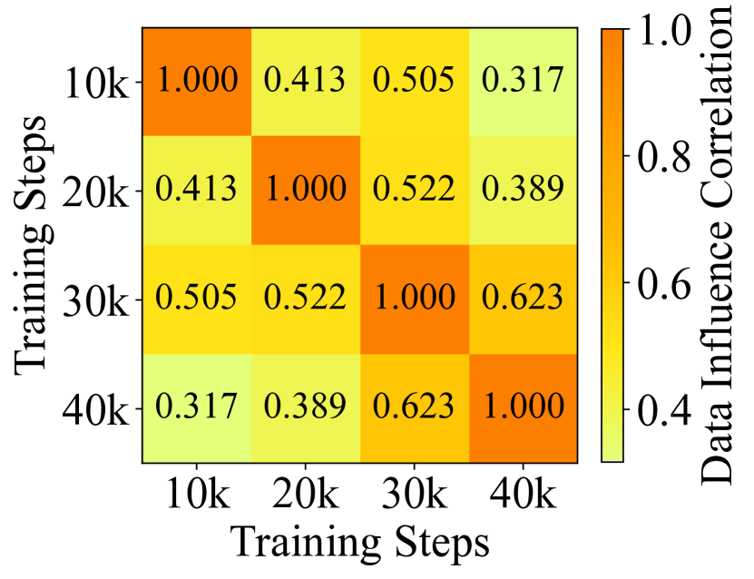
(a) Preference correlation.

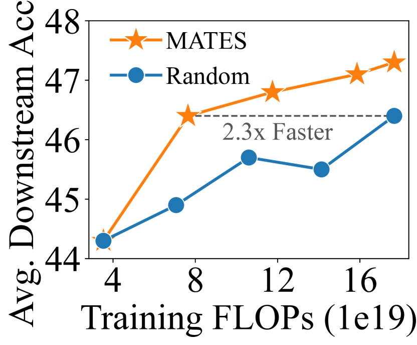
(b) Accuracy w.r.t. FLOPs.

Figure 1: Correlation of locally probed data influences at different pretraining steps (a) and the zero-shot performance with model-aware data selection (b). The experiments are based on Pythia-1B.

In this paper, we introduce Model-Aware data selection with daTa influencE modelS (MATES), a new pretraining paradigm where pretraining data is selected on-the-fly by a data influence model capturing the ever-changing data preferences of the main pretraining model. To achieve that, we locally probe the oracle data influence by evaluating the main model’s performance on a reference task after training on individual data point. Then, we use the locally collected oracle data influence scores to train a small data influence model, which then selects the data for the next pretraining stage. This side-by-side learning framework ensures that the data influence model continuously adapts to the evolving data preferences of the pretraining model, providing the most valuable data for each pretraining stage.

Our pretraining experiments with Pythia [5] on the C4 dataset [46] demonstrate that MATES can significantly outperform random selection by an average zero-shot accuracy of 1.3% across various downstream tasks, ranging from reading comprehension, commonsense reasoning, and question answering. In both zero- and few-shot settings, MATES doubles the gains obtained by state-of-the-art data selection approaches that rely on signals from reference models larger than the pretraining model. Furthermore, our model-aware data selection significantly elevates the scaling curve of pretraining models, as shown in Figure 1(b), reducing the total FLOPs required to achieve certain downstream performances by more than half.

Our experiments reveal that a small BERT-based data influence model can precisely learn the dynamic data preferences of the large decoder-only language model, and this dynamic adaptation is crucial for the effectiveness of MATES. Further analyses confirm the advantages of our locally probed oracle data influence versus influence-function-based methods [14] and the effective approximation of this oracle with data influence models. Our ablation studies demonstrate the robustness of MATES across various hyperparameter settings and different design choices of the data influence models.

We summarize our main contributions as follows:

1. We propose a model-aware data selection framework, MATES, where a small data influence model continuously adapts to the constantly changing data preferences of the pretraining model and selects the training data to optimize the efficacy of the pretraining process.

2. We effectively collect oracle data influence through local probing with the pretraining model and use a small BERT-base model to approximate it accurately.

3. We empirically verify the effectiveness of MATES over rule-based, influence-function-based, and LLM-based selection methods and the advantages of model-aware data selection.

2 Related work

Early approaches on data selection relied heavily on manual intuitions. For example, T5 [46] first proposed the C4 pipeline, followed by Gopher rules [45], which utilized criteria like document length, mean word length, and the presence of harmful or stop words to curate data. Recent FineWeb dataset [42] further applied quality and repetition filters on top of these basic rules. These rule-based data selection methods have been shown effective as an initial data curation step [42], though manual intuitions may not capture the nuances of the model’s data preferences [33].

Deduplication is another standard approach in pretraining data selection. Specifically, Lee et al. [30] and Penedo et al. [43] explored exact string match and fuzzy MinHash to filter out duplicate sequences. SemDeDup [1] further leveraged pretrained embeddings to identify semantic duplicates, and D4 [52] introduced diversification factors into the deduplication process. These methods effectively narrow down the number of similar documents in a corpus and are often used together with quality-oriented selection techniques to improve performance.

The proximity to high-quality corpora can enhance the quality of raw data as well [16; 56]. Techniques leveraging n-gram similarity [16; 58] and language modeling perplexity [8; 13; 15; 56] assessed how closely sequences in a large dataset resembled high-quality data. As the size of pretraining data grows, the effectiveness of proximity-based methods becomes unclear, as they may reduce the diversity of the pretraining data and, consequently, the capability of the pretrained models [33].

Recent advancements explore the use of LLMs to improve the pretraining data quality. For instance, QuRating [57] and Ask-LLM [47] employed LLMs like GPT-3.5 to annotate high-quality documents. Maini et al. [35] rephrased web corpora by providing LLMs with detailed prompts to balance quality and diversity. These methods leverage the capabilities of strong reference LLMs, which are often several orders of magnitude larger, to guide the pretraining of smaller models. It remains uncertain how the data curated by existing LLMs can contribute to building models stronger than them.

Influence functions [28; 54] provide a theoretical tool to assess the impact of individual data points on a model’s performance. However, they face scalability challenges in the context of LLMs due to the expensive gradient calculations [20; 49]. To efficiently and robustly approximate influence functions, TRAK [41] performed Taylor approximation and gradient dimension reduction, making influence computation feasible for pretraining experiments [14]. Nevertheless, the computational cost remains prohibitive for model-aware data selection, which requires capturing the evolving data preferences of pretraining models on the fly.

On the other hand, many researchers have proposed curriculum learning strategies that are highly effective in the pretraining [10; 23; 51; 57]. ELECTRA-style models [10] incorporated curriculum learning in their pretraining process by synchronously training the main model with an auxiliary generator, which provided more and more difficult training signals for the discriminator. This implicit curriculum significantly improved the pretraining efficiency on denoising language models [4; 10; 18; 36; 59]. Other methods have explicitly designed the curriculum for pretraining data selection, such as decreasing gradient norms [51], least certainty [23], and increasing expertise [57], demonstrating the benefits of adapting the pretraining data signal according to the model’s ever-changing preferences.

3 MATES: Model-aware data selection with data influence models

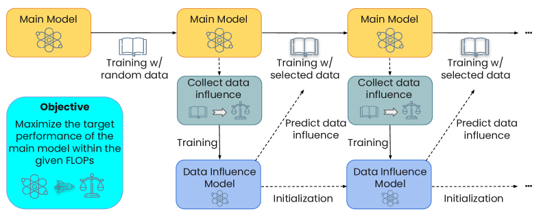
Figure 2: Overview of MATES. The main model is first pretrained with a random set of data. Then, a data influence model is trained to approximate data influences on the target performance of the main model and select the most effective data for the next pretraining stage.

This section first introduces the model-aware data selection framework MATES (§ 3.1) and then proposes a local probing technique to collect oracle data influence during pretraining (§ 3.2).

3.1 Model-aware data selection framework

Model-aware data selection combines data selection and model pretraining, aiming to maximize the model’s final target performance, as illustrated in Figure 2. The target performance here can be evaluated using any downstream task or their combinations. Specifically, we leverage data that is not part of the downstream evaluation to act as a reference for the model’s downstream performance and select the pretraining data according to the reference loss.

Formally, given a size-$n$ pretraining dataset $\mathcal{D}_{t}$ and the current model state $\mathcal{M}$, in each iteration, the objective of data selection is to find an optimal batch $B^{*}$ from $\mathcal{D}_{t}$ to minimize the loss $\mathcal{L}$ over the reference data $\mathcal{D}_{r}$ after training $\mathcal{M}$ on $B^{*}$:

$$B^{*} ={\arg\min}_{B}~{}\mathcal{L}(\mathcal{D}_{r}\mid\mathcal{A}(\mathcal{M},B))$$ (1)

$$\text{where}~{}\mathcal{L}(\mathcal{D}_{r}\mid\mathcal{A}( \mathcal{M},B))=\mathbb{E}_{(x,y)\sim\mathcal{D}_{r}}\ell(y\mid x;\mathcal{A}(\mathcal{M},B)),$$ (2)

$$\mathcal{M} \leftarrow\mathcal{A}(\mathcal{M},B^{*}),$$ (3)

where $\mathcal{A}(\mathcal{M},B)$ denotes the optimization of model $\mathcal{M}$ on a batch $B$, e.g., one-step training with Adam [27] and $\ell$ denotes the function to compute the model loss on an input-output pair $(x,y)$.

There are two challenges to implement this framework. First, enumerating all possible batches will exponentially increase computational complexity. Second, obtaining oracle data influence for all pretraining data points is costly. To address these issues, we introduce two techniques: pointwise data influence and data influence parameterization.

Algorithm 1 Model-Aware Data Selection

Training data $\mathcal{D}_{t}$, hold-out data $\mathcal{D}_{h}$, reference data $\mathcal{D}_{r}$, main model $\mathcal{M}$, optimizer $\mathcal{A}$, total training step $T$, selected size $k$, data influence model $\Theta$, sampling temperature $\tau$, update step $U$

Initialize main model parameters $\mathcal{M}$

Initialize $S_{k}^{*}$ as a randomly sampled size-$k$ subset from $\mathcal{D}_{t}$

for $t=1,\dots,T$ do

     if $t\mod U=0$ then

         Collect oracle data influence $\{\mathcal{I}_{\mathcal{M}}(x_{i};\mathcal{D}_{r})\mid x_{i}\in\mathcal{D}_{h}\}$

         Fine-tune data influence model $\Theta$ on $\{(x_{i},\mathcal{I}_{\mathcal{M}}(x_{i};\mathcal{D}_{r}))\mid x_{i}\in\mathcal{D}_{h}\}$

         Select data $S_{k}^{*}\leftarrow\{\text{Gumbel-Top-}k(\frac{\Theta(x_{i})}{\tau})\mid x_{i}\in\mathcal{D}_{t}\}$

     end if

     Sample a batch of data $B^{*}$ from $S_{k}^{*}$

     $\mathcal{M}$ $\leftarrow$ $\mathcal{A}(\mathcal{M},B^{*})$

end for

Pointwise Data Influence. To avoid the computationally intensive task of enumerating all possible batches, a more practical workaround is to decompose the group influence into the pointwise influence [14; 41]. Following previous research [41], we aggregate all the data influences by the summation, assuming that each data point $x_{i}$ has an independent influence irrespective of the others:

$$\centering\begin{split}\mathcal{L}(\mathcal{D}_{r}\mid\mathcal{A}(\mathcal{M},B))=\sum_{x_{i}\in B}\mathcal{I}_{\mathcal{M}}(x_{i};\mathcal{D}_{r}),\end{split}\@add@centering$$ (4)

where $\mathcal{I}_{\mathcal{M}}$ is the oracle pointwise data influence function based on model state $\mathcal{M}$. $\mathcal{I}_{\mathcal{M}}$ continuously changes along with the model pretraining.

Data Influence Parameterization. Estimating oracle pointwise data influence normally involves gradient-based calculation [20; 28; 41], which is impractical to perform over millions of pretraining examples for each model state. Instead, we propose to collect the oracle data influence on a small hold-out dataset $\mathcal{D}_{h}$ (sampled from the same distribution as $\mathcal{D}_{t}$) and fine-tune a small data influence model $\Theta$ on $\{(x_{i},\mathcal{I}_{\mathcal{M}}(x_{i};\mathcal{D}_{r}))\mid x_{i}\in\mathcal{D}_{h}\}$ to learn the model-aware data influence. This data influence parameterization process transfers the costly influence computation to the model forward.

Then, we run inference with the fine-tuned data influence model over all the training examples $x_{i}\in\mathcal{D}_{t}$ to obtain the influence prediction $\Theta(x_{i})$. For better efficiency, we only asynchronously update the data influence model every $U$ steps with the new oracle $\mathcal{I}_{\mathcal{M}}$ so that one data influence model checkpoint can select the entire data subset $S_{k}^{*}$ instead of one batch for the next $U$ steps of pretraining. The selection is performed using the Gumbel-Top-$k$ algorithm [29; 57]:

$$S_{k}^{*}\leftarrow\{\text{Gumbel-Top-}k(\frac{\Theta(x_{i})}{\tau})\mid x_{i}\in\mathcal{D}_{t}\}.$$ (5)

The update step $U$ is chosen to balance the efficiency of data selection with the evolving oracle data influence. We warm up the model with a random subset in the initial $U$ steps. The overall side-by-side training pipeline in MATES is described in Algorithm 1.

3.2 Locally probed oracle data influence

The next part of this section presents our method to probe the oracle data influence $\mathcal{I}_{\mathcal{M}}$. We start the derivation from the standard influence functions [28; 54] that quantify the reference loss change if one data point $x_{i}$ is upweighted by a small $\epsilon$. We denote the optimal model state after the upweighting as $\mathcal{M^{*}}_{\epsilon,x_{i}}=\mathop{\arg\min}_{\mathcal{M}}\frac{1}{n}\sum_{j=1}^{n}\mathcal{L}(x_{j}\mid\mathcal{M})+\epsilon\mathcal{L}(x_{i}\mid\mathcal{M})$ and simplify the optimal model under $\epsilon=0$ case (i.e., no upweighting) as $\mathcal{M^{*}}$. Then, the influence of upweighting $x_{i}$ is given by:

$$\mathcal{I}_{\mathcal{M^{*}}}(x_{i};\mathcal{D}_{r}) \stackrel{{\scriptstyle\mathclap{\tiny\mbox{def}}}}{{=}}\frac{d\mathcal{L}(\mathcal{D}_{r}\mid\mathcal{M^{*}}_{\epsilon,x_{i}})}{d\epsilon}|_{\epsilon=0}$$ (6)

$$=\nabla_{\mathcal{M}}\mathcal{L}(\mathcal{D}_{r}\mid\mathcal{M^{*}})^{\top}\frac{d\mathcal{M^{*}}_{\epsilon,x_{i}}}{d\epsilon}|_{\epsilon=0}$$ (7)

$$=-\nabla_{\mathcal{M}}\mathcal{L}(\mathcal{D}_{r}\mid\mathcal{M^{*}})^{\top}H_{\mathcal{M^{*}}}^{-1}\nabla_{\mathcal{M}}\mathcal{L}(x_{i}\mid\mathcal{M^{*}}),$$ (8)

where $H_{\mathcal{M^{*}}}=\frac{1}{n}\sum_{j=1}^{n}\nabla^{2}_{\mathcal{M}}\mathcal{L}(x_{j}\mid\mathcal{M^{*}})$ is the Hessian and and is positive definite. It is introduced by building a quadratic approximation to the empirical risk around $\mathcal{M^{*}}$ and taking a single Newton step [28]. Now consider the case that we remove the $x_{i}$ from the training data, which means $\epsilon=-\frac{1}{n}$, then the parameter difference due to the exclusion of $x_{i}$ is $\mathcal{M^{*}}_{-\frac{1}{n},x_{i}}-\mathcal{M^{*}}\approx-\frac{1}{n}H_{\mathcal{M^{*}}}^{-1}\nabla_{\mathcal{M}}\mathcal{L}(x_{i}\mid\mathcal{M^{*}})$ and the influence in Eq. 8 can be further represented as:

$$\mathcal{I}_{\mathcal{M^{*}}}(x_{i};\mathcal{D}_{r}) \approx n\nabla_{\mathcal{M}}\mathcal{L}(\mathcal{D}_{r}\mid\mathcal{M^{*}})^{\top}(\mathcal{M^{*}}_{-\frac{1}{n},x_{i}}-\mathcal{M^{*}})$$ (9)

$$\approx n(\mathcal{L}(\mathcal{D}_{r}\mid\mathcal{M^{*}}_{-\frac{1}{n},x_{i}})-\mathcal{L}(\mathcal{D}_{r}\mid\mathcal{M^{*}}))$$ (10)

$$\propto\mathcal{L}(\mathcal{D}_{r}\mid\mathcal{M^{*}}_{-\frac{1}{n},x_{i}})-\mathcal{L}(\mathcal{D}_{r}\mid\mathcal{M^{*}}).$$ (11)

In practice, we manage to obtain the data influence based on the current model state $\mathcal{M}$, while the above influence calculation still remains meaningful in the non-converged state by adding a damping term $\lambda$ that ensures $H_{\mathcal{M}}+\lambda I$ is positive definite [28]. Under this assumption, the first term in Eq. 11 can be regarded as a fixed value $\mathcal{L}(\mathcal{D}_{r}\mid\mathcal{M})$ whatever $x_{i}$ is, since $x_{i}$ is sampled from the hold-out data $\mathcal{D}_{h}$. The second term in Eq. 11 can be locally probed with the one-step training of the current model with the new $x_{i}$, i.e., $\mathcal{A}(\mathcal{M},x_{i}))$. This one-step training incorporates the information of $x_{i}$ into the optimization of the current model. Finally, the locally probed oracle data influence of $x_{i}$ is:

$$\mathcal{I}_{\mathcal{M}}(x_{i};\mathcal{D}_{r})\propto-\mathcal{L}(\mathcal{D}_{r}\mid\mathcal{A}(\mathcal{M},x_{i})).$$ (12)

This means, for each $x_{i}$ in the hold-out data $\mathcal{D}_{h}$, we run one-step training with the current model $\mathcal{M}$ and evaluate the reference loss with the updated model. The negative reference loss, $-\mathcal{L}(\mathcal{D}_{r}\mid\mathcal{A}(\mathcal{M},x_{i}))$, will serve as our locally probed oracle data influence.

4 Experimental methodologies

Implementation Details. We use Pythia-410M/1B [5] as our main pretraining model and fine-tune BERT-base [12] as our data influence model. The latter is smaller than the main model, ensuring the efficiecy of data selection. We continuously fine-tune the BERT model with regression modeling alongside the main model training. The learning outcome of our data influence model is evaluated by the validation Spearman correlation between its predictions and the oracle data influence. More details can be found in Appendix A.1.

For the main model (Pythia), we set the sequence length to 1024, the batch size to 512, and the max learning rate to 0.001. We take the selection size $k$ as 20% of the selection pool and the update step $U$ as 20% of the total training steps so that the selected data is trained by one epoch. Following DsDm [14], we leverage LAMBADA [40] as our reference task $\mathcal{D}_{r}$. LAMBADA is a widely-used language modeling task and often serves as a validation task for language model pretraining [7; 8; 22]. The sampling temperature $\tau$ is set to 1.0 to balance the diversity as well as the quality. For the scheduler, we utilize the Warmup-Stable-Decay (WSD) proposed in MiniCPM [24], which can converge better and faster than the Cosine scheduler [21]. The details of the WSD scheduler can be found in Appendix A.1.

Evaluation Methods. We use lm-evaluation-harness [17] codebase to perform a holistic evaluation of pretrained models across 9 downstream tasks, including SciQ [55], ARC-E [11], ARC-C [11], LogiQA [32], OBQA [38], BoolQ [9], HellaSwag [60], PIQA [6], and WinoGrande [48]. These tasks cover the core abilities of the pretrained language model, ranging from reading comprehension, commonsense reasoning, and question answering. We report normalized accuracy if the evaluation results include this metric; otherwise, we report standard accuracy. To measure inherent knowledge as well as in-context learning abilities, we evaluate the models in both zero- and two-shot manners. We also report the total GPU FLOPs, including data selection, as it is part of the scaling formulae [19].

Baselines. We compare MATES with random selection as well as the state-of-the-art pretraining data selection baselines, which include (1) DSIR [58]: proximity with Wikipedia by n-gram features. (2) SemDeDup [1]: removal of semantically duplicate sentences. (3) DsDm [14]: static approximation of influence scores on LAMBADA by a well-trained proxy model [44]. (4) QuRating [57]: ranking with Llama-learned quality scores given by GPT-3.5. These baselines cover all the mainstream data selection schemes, ranging from simple heuristics, static influence functions, and LLM rating. Some recent methods, such as Ask-LLM [47], are not open-sourced yet, prohibiting direct comparisons.

Table 1: Zero-/Two-shot evaluation of pretraining Pythia-410M/1B with different data selection methods. We report the accuracy${}_{\pm\text{standard error}}$ and the total GPU FLOPs for each method. Dependencies on stronger reference models (e.g., GPT-3.5) are denoted by $*$. Best performances are marked bold.

Methods${}_{\text{ (\#FLOPs $*$1e19)}}$	SciQ	ARC-E	ARC-C	LogiQA	OBQA
Pythia-410M
Random${}_{\text{ (6.35)}}$	$\text{64.1}_{\pm\text{1.5}}/\text{70.6}_{\pm\text{1.4}}$	$\text{40.2}_{\pm\text{1.0}}/\text{42.6}_{\pm\text{1.0}}$	$\text{{25.6}}_{\pm\text{1.3}}/\text{{25.3}}_{\pm\text{1.3}}$	$\text{24.7}_{\pm\text{1.7}}/\text{24.1}_{\pm\text{1.7}}$	$\text{29.4}_{\pm\text{2.0}}/\text{28.6}_{\pm\text{2.0}}$
DSIR${}_{\text{ (6.35)}}$	$\text{63.1}_{\pm\text{1.5}}/\text{71.4}_{\pm\text{1.4}}$	$\text{39.9}_{\pm\text{1.0}}/\text{42.0}_{\pm\text{1.0}}$	$\text{23.8}_{\pm\text{1.2}}/\text{23.6}_{\pm\text{1.2}}$	$\text{27.0}_{\pm\text{1.7}}/\text{{26.1}}_{\pm\text{1.7}}$	$\text{28.4}_{\pm\text{2.0}}/\text{28.6}_{\pm\text{2.0}}$
SemDeDup${}_{\text{ (7.81)}}$	$\text{63.5}_{\pm\text{1.5}}/\text{73.0}_{\pm\text{1.4}}$	$\text{{42.4}}_{\pm\text{1.0}}/\text{{44.5}}_{\pm\text{1.0}}$	$\text{24.4}_{\pm\text{1.3}}/\text{24.7}_{\pm\text{1.3}}$	$\text{{27.6}}_{\pm\text{1.8}}/\text{24.4}_{\pm\text{1.7}}$	$\text{30.0}_{\pm\text{2.1}}/\text{29.4}_{\pm\text{2.0}}$
DsDm${}_{\text{ (10.72)}}$	$\text{65.4}_{\pm\text{1.5}}/\text{74.0}_{\pm\text{1.4}}$	$\text{41.7}_{\pm\text{1.0}}/\text{44.2}_{\pm\text{1.0}}$	$\text{24.7}_{\pm\text{1.3}}/\text{23.6}_{\pm\text{1.2}}$	$\text{27.5}_{\pm\text{1.8}}/\text{23.5}_{\pm\text{1.7}}$	$\text{29.0}_{\pm\text{2.0}}/\text{29.2}_{\pm\text{2.0}}$
QuRating∗${}_{\text{ (26.35)}}$	$\text{64.8}_{\pm\text{1.5}}/\text{74.1}_{\pm\text{1.4}}$	$\text{42.0}_{\pm\text{1.0}}/\text{43.9}_{\pm\text{1.0}}$	$\text{25.4}_{\pm\text{1.3}}/\text{23.6}_{\pm\text{1.2}}$	$\text{25.3}_{\pm\text{1.7}}/\text{{26.1}}_{\pm\text{1.7}}$	$\text{30.2}_{\pm\text{2.1}}/\text{30.2}_{\pm\text{2.1}}$
MATES (Ours)${}_{\text{ (8.11)}}$	$\text{{66.0}}_{\pm\text{1.5}}/\text{{74.9}}_{\pm\text{1.4}}$	$\text{41.8}_{\pm\text{1.0}}/\text{43.8}_{\pm\text{1.0}}$	$\text{25.0}_{\pm\text{1.3}}/\text{{25.3}}_{\pm\text{1.3}}$	$\text{25.7}_{\pm\text{1.7}}/\text{24.9}_{\pm\text{1.7}}$	$\text{{30.8}}_{\pm\text{2.1}}/\text{{30.6}}_{\pm\text{2.1}}$
Pythia-1B
Random${}_{\text{ (17.67)}}$	$\text{65.8}_{\pm\text{1.5}}/\text{74.6}_{\pm\text{1.4}}$	$\text{43.7}_{\pm\text{1.0}}/\text{45.1}_{\pm\text{1.0}}$	$\text{25.6}_{\pm\text{1.3}}/\text{25.5}_{\pm\text{1.3}}$	$\text{27.5}_{\pm\text{1.8}}/\text{24.6}_{\pm\text{1.7}}$	$\text{31.8}_{\pm\text{2.1}}/\text{30.0}_{\pm\text{2.1}}$
MATES (Ours)${}_{\text{ (19.97)}}$	$\text{{67.3}}_{\pm\text{1.5}}/\text{{75.7}}_{\pm\text{1.4}}$	$\text{{44.9}}_{\pm\text{1.0}}/\text{{46.1}}_{\pm\text{1.0}}$	$\text{{25.9}}_{\pm\text{1.3}}/\text{{26.8}}_{\pm\text{1.3}}$	$\text{{28.7}}_{\pm\text{1.8}}/\text{{25.2}}_{\pm\text{1.7}}$	$\text{{32.2}}_{\pm\text{2.1}}/\text{{30.6}}_{\pm\text{2.1}}$
Methods${}_{\text{ (\#FLOPs $*$1e19)}}$	BoolQ	HellaSwag	PIQA	WinoGrande	Average
Pythia-410M
Random${}_{\text{ (6.35)}}$	$\text{58.9}_{\pm\text{0.9}}/\text{56.4}_{\pm\text{0.9}}$	$\text{39.7}_{\pm\text{0.5}}/\text{39.9}_{\pm\text{0.5}}$	$\text{67.1}_{\pm\text{1.1}}/\text{66.9}_{\pm\text{1.1}}$	$\text{50.6}_{\pm\text{1.4}}/\text{52.2}_{\pm\text{1.4}}$	$\text{44.5}_{\pm\text{1.3}}/\text{45.2}_{\pm\text{1.3}}$
DSIR${}_{\text{ (6.35)}}$	$\text{58.3}_{\pm\text{0.9}}/\text{56.7}_{\pm\text{0.9}}$	$\text{39.6}_{\pm\text{0.5}}/\text{39.8}_{\pm\text{0.5}}$	$\text{66.8}_{\pm\text{1.1}}/\text{66.1}_{\pm\text{1.1}}$	$\text{51.5}_{\pm\text{1.4}}/\text{51.6}_{\pm\text{1.4}}$	$\text{44.3}_{\pm\text{1.3}}/\text{45.1}_{\pm\text{1.3}}$
SemDeDup${}_{\text{ (7.81)}}$	$\text{58.2}_{\pm\text{0.9}}/\text{54.9}_{\pm\text{0.9}}$	$\text{40.8}_{\pm\text{0.5}}/\text{{40.8}}_{\pm\text{0.5}}$	$\text{67.8}_{\pm\text{1.1}}/\text{{67.6}}_{\pm\text{1.1}}$	$\text{52.3}_{\pm\text{1.4}}/\text{51.1}_{\pm\text{1.4}}$	$\text{45.2}_{\pm\text{1.4}}/\text{45.6}_{\pm\text{1.3}}$
DsDm${}_{\text{ (10.72)}}$	$\text{57.5}_{\pm\text{0.9}}/\text{54.7}_{\pm\text{0.9}}$	$\text{40.3}_{\pm\text{0.5}}/\text{40.1}_{\pm\text{0.5}}$	$\text{68.1}_{\pm\text{1.1}}/\text{66.5}_{\pm\text{1.1}}$	$\text{50.1}_{\pm\text{1.4}}/\text{51.5}_{\pm\text{1.4}}$	$\text{44.9}_{\pm\text{1.4}}/\text{45.3}_{\pm\text{1.3}}$
QuRating∗${}_{\text{ (26.35)}}$	$\text{58.9}_{\pm\text{0.9}}/\text{54.1}_{\pm\text{0.9}}$	$\text{40.7}_{\pm\text{0.5}}/\text{40.4}_{\pm\text{0.5}}$	$\text{67.5}_{\pm\text{1.1}}/\text{67.4}_{\pm\text{1.1}}$	$\text{52.1}_{\pm\text{1.4}}/\text{51.4}_{\pm\text{1.4}}$	$\text{45.2}_{\pm\text{1.4}}/\text{45.7}_{\pm\text{1.3}}$
MATES (Ours)${}_{\text{ (8.11)}}$	$\text{{60.6}}_{\pm\text{0.9}}/\text{{57.4}}_{\pm\text{0.9}}$	$\text{{41.0}}_{\pm\text{0.5}}/\text{40.6}_{\pm\text{0.5}}$	$\text{{68.7}}_{\pm\text{1.1}}/\text{67.1}_{\pm\text{1.1}}$	$\text{{52.7}}_{\pm\text{1.4}}/\text{{53.4}}_{\pm\text{1.4}}$	$\text{{45.8}}_{\pm\text{1.4}}/\text{{46.4}}_{\pm\text{1.3}}$
Pythia-1B
Random${}_{\text{ (17.67)}}$	$\text{60.2}_{\pm\text{0.9}}/\text{56.8}_{\pm\text{0.9}}$	$\text{43.8}_{\pm\text{0.5}}/\text{42.9}_{\pm\text{0.5}}$	$\text{68.9}_{\pm\text{1.1}}/\text{68.3}_{\pm\text{1.1}}$	$\text{50.7}_{\pm\text{1.4}}/\text{{52.1}}_{\pm\text{1.4}}$	$\text{46.4}_{\pm\text{1.4}}/\text{46.7}_{\pm\text{1.3}}$
MATES (Ours)${}_{\text{ (19.97)}}$	$\text{{60.9}}_{\pm\text{0.9}}/\text{{58.1}}_{\pm\text{0.9}}$	$\text{{45.3}}_{\pm\text{0.5}}/\text{{44.8}}_{\pm\text{0.5}}$	$\text{{69.5}}_{\pm\text{1.1}}/\text{{68.7}}_{\pm\text{1.1}}$	$\text{{52.4}}_{\pm\text{1.4}}/\text{51.6}_{\pm\text{1.4}}$	$\text{{47.5}}_{\pm\text{1.4}}/\text{{47.5}}_{\pm\text{1.3}}$

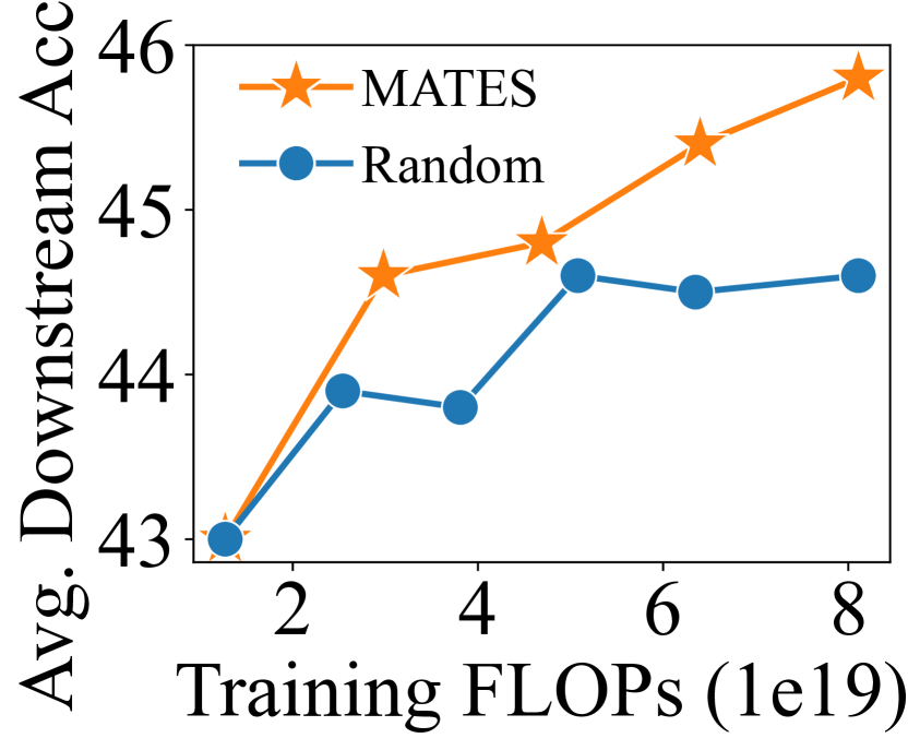
(a) 410M w/ FLOPs.

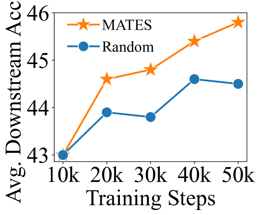
(b) 410M w/ steps.

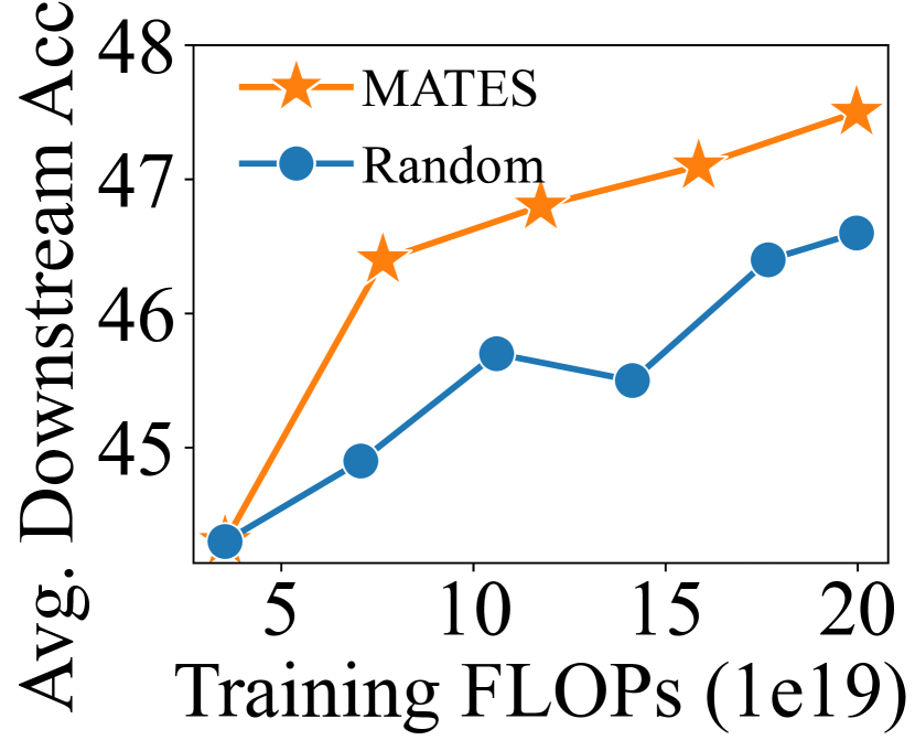
(c) 1B w/ FLOPs.

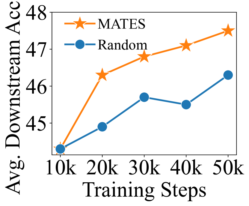
(d) 1B w/ steps.

Figure 3: Downstream zero-shot performance of Pythia-410M/1B w.r.t. pretraining FLOPs and steps. Data selection accounts for 21.7% and 11.5% of the FLOPs for 410M and 1B models, respectively.

5 Evaluation results

This section evaluates the effectiveness of MATES (§ 5.1), model-aware data selection (§ 5.2), locally probed oracle data influence (§ 5.3), and analyzes the design choices of data influence models (§ 5.4).

5.1 Overall performance

Table 1 presents the zero-/two-shot evaluation of pretraining Pythia-410M/1B with different data selection methods. With Pythia-410M, MATES significantly outperform random selection in both settings–doubling the gains obtained by the state-of-the-art data selection approach, QuRating. Notably, we observe an absolute improvement of nearly 2.0% across most tasks, except for the challenging ARC-C and LogiQA, where the predictions of 410M models are close to random guessing (25.0 accuracy). The trends hold with the larger model, Pythia-1B, with similar consistent improvements from MATES over random data selection.

Figure 3 plots the performance of the pretraining models w.r.t. different FLOPs and steps. Measuring by steps reflects the compute cost of the main model alone, as the data selection side can be trivially parallelized when more computational resources are available. Measuring by FLOPs counts both the main model and data selection costs, demonstrating the total pretraining compute budget. At both the 410M and 1B scales, MATES significantly elevates the scaling curves compared to random selection, reducing the FLOPs and pretraining steps required to reach a certain downstream performance by more than half. Scaling efficiency is more evident at the larger scale (1B), where the main model pretraining dominates 88.5% of FLOPs versus the 11.5% for the data selection. These results reveal the promising potential of MATES in elevating the scaling law of foundation models.

5.2 Effectiveness of model-aware data selection

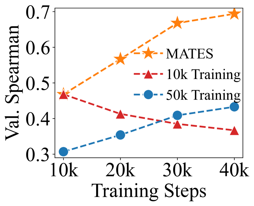
(a) Influence modeling.

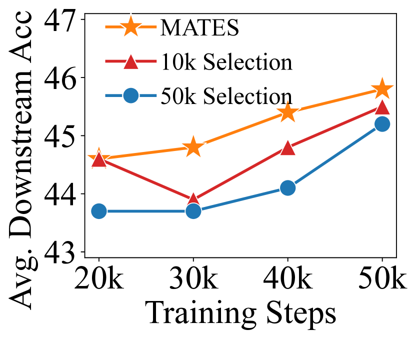
(b) Downstream accuracy.

Figure 4: Static (based on a 10k or a 50k random-pretrained model checkpoint) data selection versus model-aware data selection in influence modeling and downstream accuracy.

This experiment studies the effectiveness of model-aware data selection. Figure 4 compares MATES with static data influence models trained on influence from a 10k or a 50k random-pretrained model checkpoint. In Figure 4(a), we measure the validation Spearman correlation between the predictions of data influence models and the oracle data influence probed with each pretraining checkpoint. The correlations of static data influence models are always below 0.5, while data influence models in MATES, with dynamic updates, can capture the ever-changing data preferences more and more precisely along with the main model pretraining (e.g., the correlation is around 0.7 in 40k steps). The effects of model-aware data selection are directly reflected in downstream accuracy. In Figure 4(b), the data selected by static data influence models will cause a notable performance drop, especially at the early pretraining stage. These observations confirm the ever-changing nature of data preferences and the necessity of model-aware data selection to elevate the scaling curves of pretraining.

5.3 Effectiveness of locally probed oracle data influence

Table 2: Performances of locally probed oracle data influence, MATES, and DsDm at 40k steps.

Methods	SciQ	ARC-E	ARC-C	LogiQA	OBQA
Oracle	$\text{65.4}_{\pm\text{1.5}}/\text{70.4}_{\pm\text{1.4}}$	$\text{{42.5}}_{\pm\text{1.0}}/\text{43.6}_{\pm\text{1.0}}$	$\text{{25.2}}_{\pm\text{1.3}}/\text{25.0}_{\pm\text{1.3}}$	$\text{26.1}_{\pm\text{1.7}}/\text{25.7}_{\pm\text{1.7}}$	$\text{{31.8}}_{\pm\text{2.1}}/\text{{30.4}}_{\pm\text{2.1}}$
MATES	$\text{{67.3}}_{\pm\text{1.5}}/\text{{76.7}}_{\pm\text{1.3}}$	$\text{41.7}_{\pm\text{1.0}}/\text{{44.4}}_{\pm\text{1.0}}$	$\text{24.7}_{\pm\text{1.3}}/\text{24.0}_{\pm\text{1.2}}$	$\text{{26.9}}_{\pm\text{1.7}}/\text{{26.3}}_{\pm\text{1.7}}$	$\text{28.8}_{\pm\text{2.0}}/\text{28.0}_{\pm\text{2.0}}$
DsDm	$\text{66.0}_{\pm\text{1.5}}/\text{72.7}_{\pm\text{1.4}}$	$\text{41.7}_{\pm\text{1.0}}/\text{43.2}_{\pm\text{1.0}}$	$\text{23.7}_{\pm\text{1.2}}/\text{{25.2}}_{\pm\text{1.3}}$	$\text{24.4}_{\pm\text{1.7}}/\text{23.3}_{\pm\text{1.7}}$	$\text{29.2}_{\pm\text{2.0}}/\text{29.4}_{\pm\text{2.0}}$
Methods	BoolQ	HellaSwag	PIQA	WinoGrande	Average
Oracle	$\text{58.9}_{\pm\text{0.9}}/\text{{59.1}}_{\pm\text{0.9}}$	$\text{{41.1}}_{\pm\text{0.5}}/\text{{43.1}}_{\pm\text{0.5}}$	$\text{{68.2}}_{\pm\text{1.1}}/\text{66.6}_{\pm\text{1.1}}$	$\text{51.6}_{\pm\text{1.4}}/\text{{53.2}}_{\pm\text{1.4}}$	$\text{{45.6}}_{\pm\text{1.4}}/\text{{46.3}}_{\pm\text{1.3}}$
MATES	$\text{59.6}_{\pm\text{0.9}}/\text{57.0}_{\pm\text{0.9}}$	$\text{40.1}_{\pm\text{0.5}}/\text{39.6}_{\pm\text{0.5}}$	$\text{67.6}_{\pm\text{1.1}}/\text{{67.7}}_{\pm\text{1.1}}$	$\text{{52.1}}_{\pm\text{1.4}}/\text{51.3}_{\pm\text{1.4}}$	$\text{45.4}_{\pm\text{1.3}}/\text{46.1}_{\pm\text{1.3}}$
DsDm	$\text{{60.3}}_{\pm\text{0.9}}/\text{58.1}_{\pm\text{0.9}}$	$\text{40.4}_{\pm\text{0.5}}/\text{40.2}_{\pm\text{0.5}}$	$\text{67.2}_{\pm\text{1.1}}/\text{66.5}_{\pm\text{1.1}}$	$\text{50.4}_{\pm\text{1.4}}/\text{52.2}_{\pm\text{1.4}}$	$\text{44.8}_{\pm\text{1.3}}/\text{45.6}_{\pm\text{1.3}}$

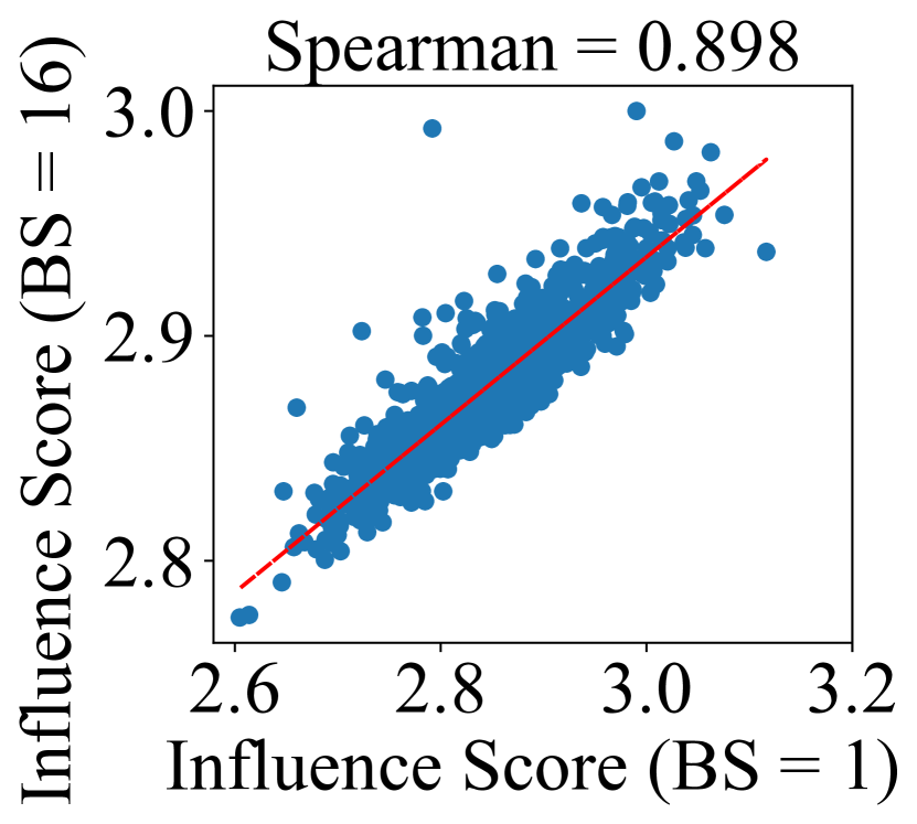
(a) Batch size (BS).

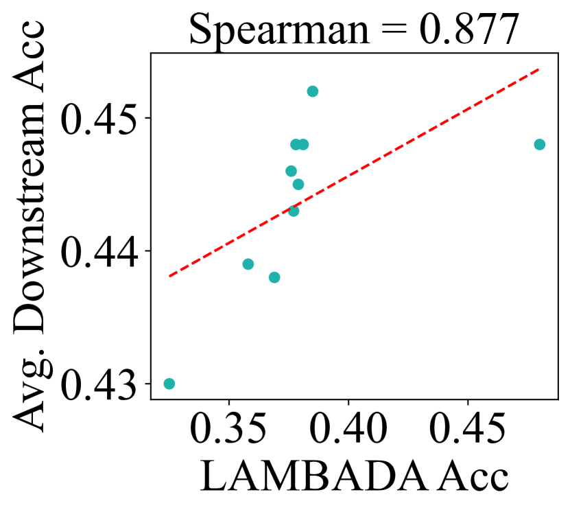
(b) LAMBADA as $\mathcal{D}_{r}$.

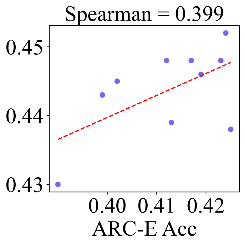
(c) ARC-E as $\mathcal{D}_{r}$.

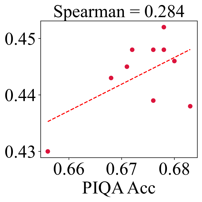
(d) PIQA as $\mathcal{D}_{r}$.

Figure 5: Correlation of oracle data influence probed with different batch sizes (a) and the correlation between different reference task accuracy with average downstream accuracy (b-d).

This set of experiments analyzes the effectiveness of the locally probed oracle data influence. We first illustrate the performance of data selection directly using the oracle at the short decay stage in Table 2. Our locally probed oracle outperforms DsDm, which leverages Taylor approximation and gradient dimension reduction, in terms of selection effectiveness. The performance gap (0.8/0.7 zero-/two-shot accuracy gain) is significant, considering the decay stage only consists of 200 steps. This improvement can be attributed to two factors: (1) we leverage the current model state to calculate the data influence rather than relying on an existing checkpoint like DsDm, and (2) we perform one-step training to obtain the oracle score, considering the training dynamics of the main model and eliminating the precision loss from multiple approximation manipulations in DsDm. Though it is always costly to acquire the optimal data influence oracle for the entire pretraining dataset, but our local probing method with data influence parameterization outperforms Taylor approximation with fewer FLOPs, offering a new direction for future exploration.

To further demonstrate the stability of our oracle data influence, we enlarge the one-step training batch size (BS) from 1 to 16. Following Ilyas et al. [25], we utilize LASSO regression to separate each data’s influence score in the BS = 16 setup and calculate Spearman correlation between BS = 1 and BS = 16 scores. Figure 5(a) illustrates that the oracle data influence is not sensitive to the batch size as long as they correspond to the same model state.

We also investigate the traits of our reference task, LAMBADA, when collecting oracle data influences. Specifically, we collect the task accuracy at each model checkpoint and measure the Spearman correlation between a single task and average downstream accuracy. As shown in Figure 5(b), LAMBADA has a significantly positive Spearman correlation (0.877) with average downstream accuracy. In contrast, the correlation between ARC-E/PIQA and average downstream accuracy is not high in Figure 5(c)/5(d), although they are parts of the evaluation tasks. These results imply that ARC-E/PIQA may not reflect the target performance as accurately as LAMBADA when acting as the reference.

5.4 Ablation study on data influence models

Table 3: Ablation study of pretraining Pythia-410M with different update steps $U$ and sampling temperatures $\tau$ between 40k to 50k steps. Our main setup is $U$=10k, $\tau$=1.0.

Methods	SciQ	ARC-E	ARC-C	LogiQA	OBQA
$U$=10k, $\tau$=1.0	$\text{{66.0}}_{\pm\text{1.5}}/\text{{74.9}}_{\pm\text{1.4}}$	$\text{41.8}_{\pm\text{1.0}}/\text{43.8}_{\pm\text{1.0}}$	$\text{{25.0}}_{\pm\text{1.3}}/\text{{25.3}}_{\pm\text{1.3}}$	$\text{25.7}_{\pm\text{1.7}}/\text{24.9}_{\pm\text{1.7}}$	$\text{30.8}_{\pm\text{2.1}}/\text{{30.6}}_{\pm\text{2.1}}$
$U$=5k, $\tau$=1.0	$\text{65.8}_{\pm\text{1.5}}/\text{74.6}_{\pm\text{1.4}}$	$\text{{42.2}}_{\pm\text{1.0}}/\text{44.1}_{\pm\text{1.0}}$	$\text{24.8}_{\pm\text{1.3}}/\text{25.1}_{\pm\text{1.3}}$	$\text{25.3}_{\pm\text{1.7}}/\text{25.8}_{\pm\text{1.7}}$	$\text{{31.0}}_{\pm\text{2.1}}/\text{30.0}_{\pm\text{2.1}}$
$U$=2.5k, $\tau$=1.0	$\text{65.0}_{\pm\text{1.5}}/\text{74.4}_{\pm\text{1.4}}$	$\text{41.8}_{\pm\text{1.0}}/\text{43.5}_{\pm\text{1.0}}$	$\text{24.9}_{\pm\text{1.3}}/\text{24.7}_{\pm\text{1.3}}$	$\text{27.6}_{\pm\text{1.8}}/\text{{26.4}}_{\pm\text{1.7}}$	$\text{30.6}_{\pm\text{2.1}}/\text{28.8}_{\pm\text{2.0}}$
$U$=10k, $\tau$=2.0	$\text{64.0}_{\pm\text{1.5}}/\text{72.2}_{\pm\text{1.4}}$	$\text{41.8}_{\pm\text{1.0}}/\text{{44.3}}_{\pm\text{1.0}}$	$\text{24.7}_{\pm\text{1.3}}/\text{23.5}_{\pm\text{1.2}}$	$\text{27.8}_{\pm\text{1.8}}/\text{24.9}_{\pm\text{1.7}}$	$\text{29.6}_{\pm\text{2.0}}/\text{{30.6}}_{\pm\text{2.1}}$
$U$=10k, $\tau$=0.0	$\text{65.9}_{\pm\text{1.5}}/\text{74.5}_{\pm\text{1.4}}$	$\text{41.8}_{\pm\text{1.0}}/\text{43.5}_{\pm\text{1.0}}$	$\text{24.6}_{\pm\text{1.3}}/\text{23.5}_{\pm\text{1.2}}$	$\text{{28.0}}_{\pm\text{1.8}}/\text{24.6}_{\pm\text{1.7}}$	$\text{30.0}_{\pm\text{2.1}}/\text{28.8}_{\pm\text{2.0}}$
Methods	BoolQ	HellaSwag	PIQA	WinoGrande	Average
$U$=10k, $\tau$=1.0	$\text{{60.6}}_{\pm\text{0.9}}/\text{57.4}_{\pm\text{0.9}}$	$\text{41.0}_{\pm\text{0.5}}/\text{40.6}_{\pm\text{0.5}}$	$\text{{68.7}}_{\pm\text{1.1}}/\text{67.1}_{\pm\text{1.1}}$	$\text{{52.7}}_{\pm\text{1.4}}/\text{{53.4}}_{\pm\text{1.4}}$	$\text{{45.8}}_{\pm\text{1.4}}/\text{46.4}_{\pm\text{1.3}}$
$U$=5k, $\tau$=1.0	$\text{60.3}_{\pm\text{0.9}}/\text{{58.8}}_{\pm\text{0.9}}$	$\text{{41.1}}_{\pm\text{0.5}}/\text{{40.8}}_{\pm\text{0.5}}$	$\text{68.2}_{\pm\text{1.1}}/\text{{68.1}}_{\pm\text{1.1}}$	$\text{52.5}_{\pm\text{1.4}}/\text{52.2}_{\pm\text{1.4}}$	$\text{45.7}_{\pm\text{1.4}}/\text{{46.6}}_{\pm\text{1.3}}$
$U$=2.5k, $\tau$=1.0	$\text{60.2}_{\pm\text{0.9}}/\text{57.5}_{\pm\text{0.9}}$	$\text{41.0}_{\pm\text{0.5}}/\text{40.6}_{\pm\text{0.5}}$	$\text{67.5}_{\pm\text{1.1}}/\text{67.1}_{\pm\text{1.1}}$	$\text{51.5}_{\pm\text{1.4}}/\text{51.1}_{\pm\text{1.4}}$	$\text{45.6}_{\pm\text{1.4}}/\text{46.0}_{\pm\text{1.3}}$
$U$=10k, $\tau$=2.0	$\text{56.2}_{\pm\text{0.9}}/\text{54.3}_{\pm\text{0.9}}$	$\text{40.8}_{\pm\text{0.5}}/\text{40.5}_{\pm\text{0.5}}$	$\text{67.7}_{\pm\text{1.1}}/\text{67.1}_{\pm\text{1.1}}$	$\text{52.2}_{\pm\text{1.4}}/\text{51.4}_{\pm\text{1.4}}$	$\text{45.0}_{\pm\text{1.4}}/\text{45.4}_{\pm\text{1.3}}$
$U$=10k, $\tau$=0.0	$\text{57.4}_{\pm\text{0.9}}/\text{55.8}_{\pm\text{0.9}}$	$\text{40.7}_{\pm\text{0.5}}/\text{40.6}_{\pm\text{0.5}}$	$\text{68.1}_{\pm\text{1.1}}/\text{66.8}_{\pm\text{1.1}}$	$\text{50.6}_{\pm\text{1.4}}/\text{51.1}_{\pm\text{1.4}}$	$\text{45.2}_{\pm\text{1.4}}/\text{45.5}_{\pm\text{1.3}}$

This group of experiments conducts ablation studies on the hyperparameters of data influence models.

Update Step and Sampling Temperature.

Table 3 shows the impact of hyperparameters on downstream performance. We initialize the model with the 40k-step MATES checkpoint and adopt different hyperparameters in the 40k-50k training. Decreasing the update step $U$ from 10k to 5k and 2.5k leads to little fluctuations since the model preferences may not dramatically change within 5k steps. Varying the sampling temperature $\tau$ to 2.0 and 0.0 causes decreased performances. The zero temperature extremely up-weights high-quality data, reducing data diversity, while higher temperatures like 2.0 do not sufficiently emphasize data quality. Our observations highlight the necessity of balancing quality and diversity in the data selection, which has already been verified in QuRating [57] and Ask-LLM [47].

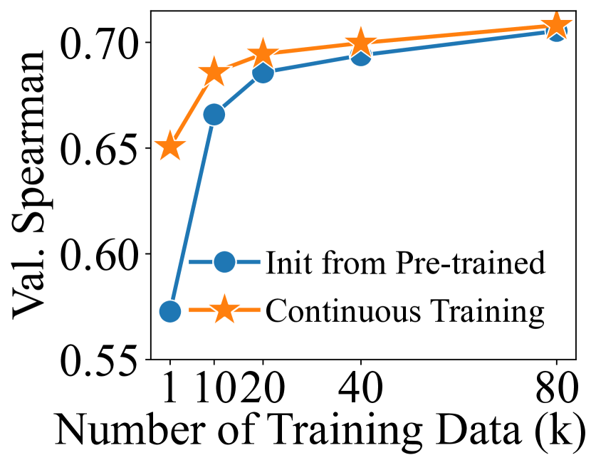
(a) Oracle label amount.

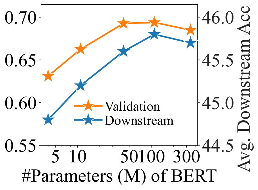
(b) Model scale.

Figure 6: Performance of data influence parameterization with different amounts of oracle labels and model scales.

Oracle Label Amount and Data Influence Model Scale.

Figure 6(a) demonstrates the impact of oracle label amounts by comparing the validation Spearman correlation of different data influence models at 40k steps. The data influence model is initialized from either the pretrained BERT or its last checkpoint at 30k steps. We observe that continuous fine-tuning from 30k steps requires less than half of the oracle data compared to training from the pretrained BERT, which can significantly reduce the cost of collecting new oracle data. Furthermore, Figure 6(b) studies the impact of parameter counts in the data influence model. Generally, the approximation becomes more accurate as the number of parameters increases until BERT-large, which may have become saturated with the current learning algorithm using the available oracle label. We have proved the effectiveness of our data influence models through extensive experiments and thus, leave the exploration of better data influence parameterization algorithms and stronger data influence models to future work.

6 Discussion and limitations

Combinational Measurement of Data Influence.

One primary assumption in our work is that each data contributes independently to the pretraining. Despite a common hypothesis [14; 41], the pretraining essentially applies the long-term combinational effect of batched data on language models, and the learning of many advanced capabilities is accumulative. Efficiently and effectively measuring and learning the combinational and accumulative nature of the pretraining process is an important direction for future research to further understand and leverage the value of data [34].

Exploratory Scale.

As an exploratory research work, our experiments are conducted at a moderate scale, with a main model of 410M or 1B parameters. Although the trend from 410M to 1B indicates the robustness of our observations, it remains unclear how well our methods scale up to production-level models with billions of parameters and trillions of pretraining tokens. On the one hand, moving to that scale provides more headroom for data selection, with more urgent needs for efficiency, more leniency on the relatively small compute spent on data selection, and a larger pool of candidate data. On the other hand, large-scale pretraining may yield various stability issues that require dedicated work to introduce new techniques [53; 61]. We leave the exploration of larger models to future work.

7 Conclusion

In this paper, we introduce MATES, a novel framework to enhance the efficiency and effectiveness of language model pretraining through model-aware data selection. MATES leverages a data influence model to continuously capture the evolving data preferences of the main model throughout the pretraining process, thereby selecting the training data most effective for the current pretraining stage. To implement that, we locally probe the oracle data influence on a reference task using the main model and fit the data influence model on the probed oracle. Our empirical results demonstrate that MATES surpasses random, rule-based, influence-function-based, and LLM-based data selection methods on pretraining, significantly elevating the scaling curves of pretraining LLMs. Further analysis confirms the necessity of model-aware data selection and the effectiveness of locally probed oracle data influence. Our work successfully demonstrates the potential of model-aware data curation in pretraining, and we hope it will motivate further explorations on improving the scaling law of foundation models through better data curation techniques.

Appendix A Appendix / supplemental material

A.1 Additional experimental details

BERT-based data influence model averages all the hidden representations of the last model layer to obtain the sequence representation $\textbf{h}\in\mathbb{R}^{H}$, where $H$ is the hidden size of the model. Note that BERT can only support a maximum input sequence length of 512. To deal with our pretraining sequence length of 1024, we divide one sequence into two chunks and forward them separately. Then, we average the hidden representations from both chunks to obtain the final h. This vector will be multiplied by a regression output weight $\textbf{w}_{o}\in\mathbb{R}^{H}$ to get the model prediction $\textbf{w}_{o}\cdot\textbf{h}$. The training objective is the mean squared error between the model prediction and the normalized ground truth $\mathcal{I}_{\mathcal{M}}$.

For the hyperparameters, we set the training epochs to 5, the batch size to 512, and the max learning rate to 5e-5. Note that BERT has a different tokenizer from the main model Pythia, but the average sequence length of all the examples after the tokenization is almost the same. Our chunk-based design can be easily extended to longer pretraining sequences in the future.

The learning rate of WSD scheduler is as follows:

$$lr(t)=\begin{cases}\frac{t}{W}\cdot\eta,&\text{if }t<W\\ \eta,&\text{if }W\leq t<S\\ 0.5^{4\cdot(t-S)/D}\cdot\eta,&\text{if }S\leq t<S+D\end{cases}$$ (13)

where $t$, $W$, $S$, and $D$ represent the number of steps now, at the end of the warmup, stable, and decay stages, respectively. $\eta$ is the max learning rate. In our main experiments, we choose $W$ = 2000, $S$ = 50000, and $D$ = 200. Inspired by MiniCPM Hu et al. [2024], each checkpoint is evaluated after the short decay stage for better stability. We run all experiments on 8 A6000 GPUs, which will take 2 days for 410M models and 4 days for 1B models.

References

- Abbas et al. [2023] Amro Abbas, Kushal Tirumala, Dániel Simig, Surya Ganguli, and Ari S Morcos. Semdedup: Data-efficient learning at web-scale through semantic deduplication. arXiv preprint arXiv:2303.09540, 2023.
- Achiam et al. [2023] Josh Achiam, Steven Adler, Sandhini Agarwal, Lama Ahmad, Ilge Akkaya, Florencia Leoni Aleman, Diogo Almeida, Janko Altenschmidt, Sam Altman, Shyamal Anadkat, et al. Gpt-4 technical report. arXiv preprint arXiv:2303.08774, 2023.
- Albalak et al. [2024] Alon Albalak, Yanai Elazar, Sang Michael Xie, Shayne Longpre, Nathan Lambert, Xinyi Wang, Niklas Muennighoff, Bairu Hou, Liangming Pan, Haewon Jeong, et al. A survey on data selection for language models. arXiv preprint arXiv:2402.16827, 2024.
- Bajaj et al. [2022] Payal Bajaj, Chenyan Xiong, Guolin Ke, Xiaodong Liu, Di He, Saurabh Tiwary, Tie-Yan Liu, Paul Bennett, Xia Song, and Jianfeng Gao. Metro: Efficient denoising pretraining of large scale autoencoding language models with model generated signals. arXiv preprint arXiv:2204.06644, 2022.
- Biderman et al. [2023] Stella Biderman, Hailey Schoelkopf, Quentin Gregory Anthony, Herbie Bradley, Kyle O’Brien, Eric Hallahan, Mohammad Aflah Khan, Shivanshu Purohit, USVSN Sai Prashanth, Edward Raff, et al. Pythia: A suite for analyzing large language models across training and scaling. In ICML, pages 2397–2430. PMLR, 2023.
- Bisk et al. [2020] Yonatan Bisk, Rowan Zellers, Jianfeng Gao, Yejin Choi, et al. Piqa: Reasoning about physical commonsense in natural language. In Proceedings of AAAI, volume 34, pages 7432–7439, 2020.
- Brown et al. [2020] Tom Brown, Benjamin Mann, Nick Ryder, Melanie Subbiah, Jared D Kaplan, Prafulla Dhariwal, Arvind Neelakantan, Pranav Shyam, Girish Sastry, Amanda Askell, et al. Language models are few-shot learners. In NeurIPS, pages 1877–1901, 2020.
- Chowdhery et al. [2022] Aakanksha Chowdhery, Sharan Narang, Jacob Devlin, Maarten Bosma, Gaurav Mishra, Adam Roberts, Paul Barham, Hyung Won Chung, Charles Sutton, Sebastian Gehrmann, Parker Schuh, and et al. Palm: Scaling language modeling with pathways. arXiv preprint arXiv:2204.02311, 2022.
- Clark et al. [2019] Christopher Clark, Kenton Lee, Ming-Wei Chang, Tom Kwiatkowski, Michael Collins, and Kristina Toutanova. Boolq: Exploring the surprising difficulty of natural yes/no questions. In Proceedings of NAACL, pages 2924–2936, 2019.
- Clark et al. [2020] Kevin Clark, Minh-Thang Luong, Quoc V. Le, and Christopher D. Manning. ELECTRA: Pre-training text encoders as discriminators rather than generators. In ICLR, 2020. URL https://openreview.net/pdf?id=r1xMH1BtvB.
- Clark et al. [2018] Peter Clark, Isaac Cowhey, Oren Etzioni, Tushar Khot, Ashish Sabharwal, Carissa Schoenick, and Oyvind Tafjord. Think you have solved question answering? try arc, the ai2 reasoning challenge. arXiv preprint arXiv:1803.05457, 2018.
- Devlin et al. [2019] Jacob Devlin, Ming-Wei Chang, Kenton Lee, and Kristina Toutanova. BERT: Pre-training of deep bidirectional transformers for language understanding. In Proceedings of NAACL, pages 4171–4186, 2019.
- Du et al. [2022] Nan Du, Yanping Huang, Andrew M Dai, Simon Tong, Dmitry Lepikhin, Yuanzhong Xu, Maxim Krikun, Yanqi Zhou, Adams Wei Yu, Orhan Firat, et al. Glam: Efficient scaling of language models with mixture-of-experts. In ICML, pages 5547–5569. PMLR, 2022.
- Engstrom et al. [2024] Logan Engstrom, Axel Feldmann, and Aleksander Madry. Dsdm: Model-aware dataset selection with datamodels. arXiv preprint arXiv:2401.12926, 2024.
- Gan et al. [2023] Ruyi Gan, Ziwei Wu, Renliang Sun, Junyu Lu, Xiaojun Wu, Dixiang Zhang, Kunhao Pan, Ping Yang, Qi Yang, Jiaxing Zhang, et al. Ziya2: Data-centric learning is all llms need. arXiv preprint arXiv:2311.03301, 2023.
- Gao et al. [2020] Leo Gao, Stella Biderman, Sid Black, Laurence Golding, Travis Hoppe, Charles Foster, Jason Phang, Horace He, Anish Thite, Noa Nabeshima, et al. The pile: An 800gb dataset of diverse text for language modeling. arXiv preprint arXiv:2101.00027, 2020.
- Gao et al. [2023] Leo Gao, Jonathan Tow, Baber Abbasi, Stella Biderman, Sid Black, Anthony DiPofi, Charles Foster, Laurence Golding, Jeffrey Hsu, Alain Le Noac’h, Haonan Li, Kyle McDonell, Niklas Muennighoff, Chris Ociepa, Jason Phang, Laria Reynolds, Hailey Schoelkopf, Aviya Skowron, Lintang Sutawika, Eric Tang, Anish Thite, Ben Wang, Kevin Wang, and Andy Zou. A framework for few-shot language model evaluation, 12 2023. URL https://zenodo.org/records/10256836.
- Gong et al. [2023] Linyuan Gong, Chenyan Xiong, Xiaodong Liu, Payal Bajaj, Yiqing Xie, Alvin Cheung, Jianfeng Gao, and Xia Song. Model-generated pretraining signals improves zero-shot generalization of text-to-text transformers. arXiv preprint arXiv:2305.12567, 2023.
- Goyal et al. [2024] Sachin Goyal, Pratyush Maini, Zachary C Lipton, Aditi Raghunathan, and J Zico Kolter. Scaling laws for data filtering–data curation cannot be compute agnostic. arXiv preprint arXiv:2404.07177, 2024.
- Grosse et al. [2023] Roger Grosse, Juhan Bae, Cem Anil, Nelson Elhage, Alex Tamkin, Amirhossein Tajdini, Benoit Steiner, Dustin Li, Esin Durmus, Ethan Perez, et al. Studying large language model generalization with influence functions. arXiv preprint arXiv:2308.03296, 2023.
- Hägele et al. [2024] Alexander Hägele, Elie Bakouch, Atli Kosson, Loubna Ben Allal, Leandro Von Werra, and Martin Jaggi. Scaling laws and compute-optimal training beyond fixed training durations. arXiv preprint arXiv:2405.18392, 2024.
- Hoffmann et al. [2022] Jordan Hoffmann, Sebastian Borgeaud, Arthur Mensch, Elena Buchatskaya, Trevor Cai, Eliza Rutherford, Diego de Las Casas, Lisa Anne Hendricks, Johannes Welbl, Aidan Clark, Thomas Hennigan, Eric Noland, Katherine Millican, George van den Driessche, Bogdan Damoc, Aurelia Guy, Simon Osindero, Karén Simonyan, Erich Elsen, Oriol Vinyals, Jack Rae, and Laurent Sifre. An empirical analysis of compute-optimal large language model training. In NeurIPS, pages 30016–30030, 2022.
- Hong et al. [2023] Xudong Hong, Sharid Loáiciga, and Asad Sayeed. A surprisal oracle for active curriculum language modeling. In Alex Warstadt, Aaron Mueller, Leshem Choshen, Ethan Wilcox, Chengxu Zhuang, Juan Ciro, Rafael Mosquera, Bhargavi Paranjabe, Adina Williams, Tal Linzen, and Ryan Cotterell, editors, Proceedings of the BabyLM Challenge at the 27th Conference on Computational Natural Language Learning, pages 259–268, Singapore, December 2023. Association for Computational Linguistics. doi: 10.18653/v1/2023.conll-babylm.22. URL https://aclanthology.org/2023.conll-babylm.22.
- Hu et al. [2024] Shengding Hu, Yuge Tu, Xu Han, Chaoqun He, Ganqu Cui, Xiang Long, Zhi Zheng, Yewei Fang, Yuxiang Huang, Weilin Zhao, et al. Minicpm: Unveiling the potential of small language models with scalable training strategies. arXiv preprint arXiv:2404.06395, 2024.
- Ilyas et al. [2022] Andrew Ilyas, Sung Min Park, Logan Engstrom, Guillaume Leclerc, and Aleksander Madry. Datamodels: Predicting predictions from training data. In ICML, 2022.
- Kaplan et al. [2020] Jared Kaplan, Sam McCandlish, Tom Henighan, Tom B Brown, Benjamin Chess, Rewon Child, Scott Gray, Alec Radford, Jeffrey Wu, and Dario Amodei. Scaling laws for neural language models. arXiv preprint arXiv:2001.08361, 2020.
- Kingma and Ba [2015] Diederik Kingma and Jimmy Ba. Adam: A method for stochastic optimization. In ICLR, San Diega, CA, USA, 2015.
- Koh and Liang [2017] Pang Wei Koh and Percy Liang. Understanding black-box predictions via influence functions. In ICML, pages 1885–1894. PMLR, 2017.
- Kool et al. [2019] Wouter Kool, Herke Van Hoof, and Max Welling. Stochastic beams and where to find them: The gumbel-top-k trick for sampling sequences without replacement. In ICML, pages 3499–3508, 2019.
- Lee et al. [2022] Katherine Lee, Daphne Ippolito, Andrew Nystrom, Chiyuan Zhang, Douglas Eck, Chris Callison-Burch, and Nicholas Carlini. Deduplicating training data makes language models better. In Smaranda Muresan, Preslav Nakov, and Aline Villavicencio, editors, Proceedings of ACL, pages 8424–8445, Dublin, Ireland, May 2022. Association for Computational Linguistics. doi: 10.18653/v1/2022.acl-long.577. URL https://aclanthology.org/2022.acl-long.577.
- Lin et al. [2024] Zhenghao Lin, Zhibin Gou, Yeyun Gong, Xiao Liu, Yelong Shen, Ruochen Xu, Chen Lin, Yujiu Yang, Jian Jiao, Nan Duan, et al. Rho-1: Not all tokens are what you need. arXiv preprint arXiv:2404.07965, 2024.
- Liu et al. [2021] Jian Liu, Leyang Cui, Hanmeng Liu, Dandan Huang, Yile Wang, and Yue Zhang. Logiqa: a challenge dataset for machine reading comprehension with logical reasoning. In Proceedings of IJCAI, pages 3622–3628, 2021.
- Longpre et al. [2023] Shayne Longpre, Gregory Yauney, Emily Reif, Katherine Lee, Adam Roberts, Barret Zoph, Denny Zhou, Jason Wei, Kevin Robinson, David Mimno, et al. A pretrainer’s guide to training data: Measuring the effects of data age, domain coverage, quality, & toxicity. arXiv preprint arXiv:2305.13169, 2023.
- Lundberg and Lee [2017] Scott M Lundberg and Su-In Lee. A unified approach to interpreting model predictions. In NeurIPS, volume 30, 2017.
- Maini et al. [2024] Pratyush Maini, Skyler Seto, He Bai, David Grangier, Yizhe Zhang, and Navdeep Jaitly. Rephrasing the web: A recipe for compute and data-efficient language modeling. arXiv preprint arXiv:2401.16380, 2024.
- Meng et al. [2021] Yu Meng, Chenyan Xiong, Payal Bajaj, Paul Bennett, Jiawei Han, Xia Song, et al. Coco-lm: Correcting and contrasting text sequences for language model pretraining. In NeurIPS, volume 34, pages 23102–23114, 2021.
- Meng et al. [2022] Yu Meng, Chenyan Xiong, Payal Bajaj, Saurabh Tiwary, Paul Bennett, Jiawei Han, and Xia Song. Pretraining text encoders with adversarial mixture of training signal generators. arXiv preprint arXiv:2204.03243, 2022.
- Mihaylov et al. [2018] Todor Mihaylov, Peter Clark, Tushar Khot, and Ashish Sabharwal. Can a suit of armor conduct electricity? a new dataset for open book question answering. In EMNLP, 2018.
- Overwijk et al. [2022] Arnold Overwijk, Chenyan Xiong, and Jamie Callan. Clueweb22: 10 billion web documents with rich information. In SIGIR, pages 3360–3362, 2022.
- Paperno et al. [2016] Denis Paperno, German David Kruszewski Martel, Angeliki Lazaridou, Ngoc Pham Quan, Raffaella Bernardi, Sandro Pezzelle, Marco Baroni, Gemma Boleda Torrent, Fernández Raquel, et al. The lambada dataset: Word prediction requiring a broad discourse context. In Proceedings of ACL, volume 3, pages 1525–1534, 2016.
- Park et al. [2023] Sung Min Park, Kristian Georgiev, Andrew Ilyas, Guillaume Leclerc, and Aleksander Mądry. Trak: attributing model behavior at scale. In ICML, pages 27074–27113, 2023.
- Penedo et al. [2024a] Guilherme Penedo, Hynek Kydlíček, Leandro von Werra, and Thomas Wolf. Fineweb, 2024a. URL https://huggingface.co/datasets/HuggingFaceFW/fineweb.
- Penedo et al. [2024b] Guilherme Penedo, Quentin Malartic, Daniel Hesslow, Ruxandra Cojocaru, Hamza Alobeidli, Alessandro Cappelli, Baptiste Pannier, Ebtesam Almazrouei, and Julien Launay. The refinedweb dataset for falcon llm: Outperforming curated corpora with web data only. In NeurIPS, volume 36, 2024b.
- Radford et al. [2019] Alec Radford, Jeff Wu, Rewon Child, David Luan, Dario Amodei, Ilya Sutskever, Jeffrey Dean, and Sanjay Ghemawat. Language models are unsupervised multitask learners. In OSDI’04: Sixth Symposium on Operating System Design and Implementation, pages 137–150, 2019.
- Rae et al. [2021] Jack W Rae, Sebastian Borgeaud, Trevor Cai, Katie Millican, Jordan Hoffmann, Francis Song, John Aslanides, Sarah Henderson, Roman Ring, Susannah Young, et al. Scaling language models: Methods, analysis & insights from training gopher. arXiv preprint arXiv:2112.11446, 2021.
- Raffel et al. [2020] Colin Raffel, Noam Shazeer, Adam Roberts, Katherine Lee, Sharan Narang, Michael Matena, Yanqi Zhou, Wei Li, and Peter J. Liu. Exploring the limits of transfer learning with a unified text-to-text transformer. JMLR, 21:140:1–140:67, 2020.
- Sachdeva et al. [2024] Noveen Sachdeva, Benjamin Coleman, Wang-Cheng Kang, Jianmo Ni, Lichan Hong, Ed H Chi, James Caverlee, Julian McAuley, and Derek Zhiyuan Cheng. How to train data-efficient llms. arXiv preprint arXiv:2402.09668, 2024.
- Sakaguchi et al. [2021] Keisuke Sakaguchi, Ronan Le Bras, Chandra Bhagavatula, and Yejin Choi. Winogrande: An adversarial winograd schema challenge at scale. Communications of the ACM, 64(9):99–106, 2021.
- Schioppa et al. [2022] Andrea Schioppa, Polina Zablotskaia, David Vilar, and Artem Sokolov. Scaling up influence functions. In Proceedings of AAAI, volume 36, pages 8179–8186, 2022.
- Soldaini et al. [2024] Luca Soldaini, Rodney Kinney, Akshita Bhagia, Dustin Schwenk, David Atkinson, Russell Authur, Ben Bogin, Khyathi Chandu, Jennifer Dumas, Yanai Elazar, Valentin Hofmann, Ananya Harsh Jha, Sachin Kumar, Li Lucy, Xinxi Lyu, Nathan Lambert, Ian Magnusson, Jacob Morrison, Niklas Muennighoff, Aakanksha Naik, Crystal Nam, Matthew E. Peters, Abhilasha Ravichander, Kyle Richardson, Zejiang Shen, Emma Strubell, Nishant Subramani, Oyvind Tafjord, Pete Walsh, Luke Zettlemoyer, Noah A. Smith, Hannaneh Hajishirzi, Iz Beltagy, Dirk Groeneveld, Jesse Dodge, and Kyle Lo. Dolma: An Open Corpus of Three Trillion Tokens for Language Model Pretraining Research. arXiv preprint, 2024. URL https://arxiv.org/abs/2402.00159.
- Thakkar et al. [2023] Megh Thakkar, Tolga Bolukbasi, Sriram Ganapathy, Shikhar Vashishth, Sarath Chandar, and Partha Talukdar. Self-influence guided data reweighting for language model pre-training. In Proceedings of EMNLP, pages 2033–2045, 2023.
- Tirumala et al. [2024] Kushal Tirumala, Daniel Simig, Armen Aghajanyan, and Ari Morcos. D4: Improving llm pretraining via document de-duplication and diversification. In NeurIPS, volume 36, 2024.
- Touvron et al. [2023] Hugo Touvron, Louis Martin, Kevin Stone, Peter Albert, Amjad Almahairi, Yasmine Babaei, Nikolay Bashlykov, Soumya Batra, Prajjwal Bhargava, Shruti Bhosale, et al. Llama 2: Open foundation and fine-tuned chat models. arXiv preprint arXiv:2307.09288, 2023.
- Weisberg and Cook [1982] Sanford Weisberg and R Dennis Cook. Residuals and influence in regression. 1982.
- Welbl et al. [2017] Johannes Welbl, Nelson F Liu, and Matt Gardner. Crowdsourcing multiple choice science questions. In Proceedings of the 3rd Workshop on Noisy User-generated Text, pages 94–106, 2017.
- Wenzek et al. [2020] Guillaume Wenzek, Marie-Anne Lachaux, Alexis Conneau, Vishrav Chaudhary, Francisco Guzmán, Armand Joulin, and Édouard Grave. Ccnet: Extracting high quality monolingual datasets from web crawl data. In Proceedings of the Twelfth Language Resources and Evaluation Conference, pages 4003–4012, 2020.
- Wettig et al. [2024] Alexander Wettig, Aatmik Gupta, Saumya Malik, and Danqi Chen. Qurating: Selecting high-quality data for training language models. arXiv preprint arXiv:2402.09739, 2024.
- Xie et al. [2023] Sang Michael Xie, Shibani Santurkar, Tengyu Ma, and Percy Liang. Data selection for language models via importance resampling. In NeurIPS, 2023.
- Xu et al. [2020] Zhenhui Xu, Linyuan Gong, Guolin Ke, Di He, Shuxin Zheng, Liwei Wang, Jiang Bian, and Tie-Yan Liu. Mc-bert: Efficient language pre-training via a meta controller. arXiv preprint arXiv:2006.05744, 2020.
- Zellers et al. [2019] Rowan Zellers, Ari Holtzman, Yonatan Bisk, Ali Farhadi, and Yejin Choi. Hellaswag: Can a machine really finish your sentence? In Proceedings of ACL, pages 4791–4800, 2019.
- Zhang et al. [2022] Susan Zhang, Stephen Roller, Naman Goyal, Mikel Artetxe, Moya Chen, Shuohui Chen, Christopher Dewan, Mona Diab, Xian Li, Xi Victoria Lin, Todor Mihaylov, Myle Ott, Sam Shleifer, Kurt Shuster, Daniel Simig, Punit Singh Koura, Anjali Sridhar, Tianlu Wang, and Luke Zettlemoyer. Opt: Open pre-trained transformer language models. arXiv preprint arXiv:2205.01068, 2022.