Delayed supermartingale convergence lemmas for stochastic approximation with Nesterov momentum

Abstract

This paper focus on the convergence of stochastic approximation with Nesterov momentum. Nesterov acceleration has proven effective in machine learning for its ability to reduce computational complexity. The issue of delayed information in the acceleration term remains a challenge to achieving the almost sure convergence. Based on the delayed supermatingale convergence lemmas, we give a series of framework for almost sure convergence. Our framework applies to several widely-used random iterative methods, such as stochastic subgradient methods, the proximal Robbins-Monro method for general stochastic optimization, and the proximal stochastic subgradient method for composite optimization. Through the applications of our framework, these methods with Nesterov acceleration achieve almost sure convergence. And three groups of numerical experiments is to check out theoretical results.

Keywords: Delayed supermartingale , Nesterov method, delayed iterative methods, almost sure convergence

1 Introduction

Stochastic approximation methods have gained significant prominence in addressing optimization challenges across diverse fields, particularly in the context of machine learning and risk management. The algorithms as stochastic gradient descent (SGD) Robbins and Monro (1951) and proximal Robbins-Monro methods Toulis et al. (2021) are well-regarded for their efficiency and memory cost. However, achieving convergence, especially for methods without an inherent delay mechanism, presents a significant challenge. In recent years, stochastic iterative methods have become notable contenders for addressing optimization issues, specially when dealing with large datasets. Moreover, the incorporation of acceleration techniques such as Nesterov’s momentum has further enhanced the efficiency and convergence speed of stochastic approximation methods, underscoring their widespread acknowledgment and applicability in various optimization packages, including keras.optimizers, paddle.optimizer, sklearn.neural_network, and torch.optim.

1.1 Stochastic approximation methods

The stochastic optimization problem can be formulated as minimizing the expected value of a function, denoted by $f(x)=\mathbb{E}[F(x,\xi)]$, where $F$ depends on both the decision variable $x$ and a random variable $\xi$. In the context of machine learning, the sheer volume of data samples often renders direct calculation of this expectation computationally expensive. Similarly, risk management, where $\xi$ might represent a continuous random variable, faces analytical intractability when determining the expectation.

Stochastic approximation methods have emerged as powerful tools to address these challenges. By iteratively sampling from the underlying distribution, these methods estimate the expected value, effectively circumventing the computational hurdles imposed by massive datasets or complex random variable structures. Consequently, stochastic approximation methods have become ubiquitous across diverse fields, including machine learning and risk management. However, the convergence rate of stochastic approximation method is slow, which the modified method is required.

1.2 Stochastic approximation methods with momentum

To further enhance the efficiency and convergence speed of stochastic approximation methods, techniques like Nesterov acceleration have been incorporated. Nesterov’s method, built on the concept of momentum-driven optimization, leverages gradient information more effectively by incorporating a smoothing component that accounts for past updates Assran and Rabbat . This integration has demonstrably improved the performance of stochastic approximation algorithms, primarily by reducing the number of iterations required to achieve a desired level of accuracy. However, it’s important to note that the effectiveness of momentum-based methods, like Nesterov acceleration, can be sensitive to the chosen parameters. For instance, using a suboptimal momentum value in Nesterov’s method might not outperform the original stochastic gradient descent Kidambi et al. (2018).

The stochastic approximation algorithm enhanced with Nesterov acceleration operates as follows:

(Step 1) $$v_{k+1}=x_{k}-\alpha_{k}g(x_{k},\xi_{k})$$

(Step 2) $$x_{k+1}=(1+\theta_{k})v_{k+1}-\theta_{k}v_{k}$$

where $g(x_{k},\xi_{k})$ denotes stochastic first-order information of the objective function, $\alpha_{k}>0$ is the step size, and $\theta_{k}$ is the momentum parameter. When $\theta_{k}\equiv 0$, it reverts to the conventional stochastic approximation approach. For $\theta_{k}\in(-1,0)$, it signifies a weighted delayed stochastic approximation variant, while $\theta_{k}\in(0,1)$ corresponds to the Nesterov accelerated stochastic approximation method, which is the focus of this paper. $v_{k}$ could be seen as a delay term for $x_{k+1}$.

Existing convergence analysis, such as the Robbins-Siegmund lemma Robbins and Siegmund (1971), have played a crucial role in establishing the almost sure convergence of other stochastic iterative methods. However, its reliance on a specific analytical framework limits its applicability to methods lacking inherent delays. Alternative approaches, such as the dynamical system perspective Benaïm et al. (2005), and recent advancements like the composite stochastic optimization coupling supermartingale and T-coupling Supermartingale Wang et al. (2017), Yang (2019), offer promising avenues for further analysis.

Previous works have extensively analyzed the efficiency of Nesterov acceleration under various conditions, including quadratic objectives Assran and Rabbat , Safavi et al. (2018) and smooth, strongly convex functions Jain et al. (2018). In the presence of smooth and strongly convex conditions, the almost sure convergence rate has been elucidated for methods with a constant momentum parameter Liu and Yuan (2022). Additionally, the convergence of the expected function value has been demonstrated for smooth and nonconvex functions Liang et al. (2023). Further research has introduced dynamical strategies for adjusting the momentum parameter Sun et al. (2021), Sun et al. (2022), while other works have proposed quasi-hyperbolic momentum related to Nesterov momentum and analyzed its almost sure convergence under smooth conditions Zhou et al. (2020). Finally, the role of memory in stochastic optimization has also been discussed in the literature Gitman et al. (2019).

1.3 Our Contributions

• Novel supermartingale convergence lemmas with delay: This paper aims to bridge the gap in the existing literature by introducing a novel approach that reveals a framework for constructing custom supermartingale sequences tailored to specific stochastic iterative methods. Unlike the classical stochastic approximation, the almost sure convergence of stochastic approximation with Nesterov momentum require different versions of the supermatingale convergence lemmas.

• Almost sure convergence for stochastic subgradient method with Nesterov momentum By leveraging the ”delay” structure, we provide a novel insight into the almost sure convergence for Nesterov accelerated stochastic approximation without differentiable assumptions. Projection operator onto convex set is also allowed.

• Almost sure convergence for proximal methods with Nesterov momentum Nesterov accelerated proximal Robbins-Monro methods obtains almost sure convergence. For composite optimization, proximal stochastic subgradient method with Nesterov momentum also obtains almost sure convergence.

The rest of this paper is organized as follows. In section 2, a convergence lemma for supermartingales with delay term is presented, which serves as the theoretical foundation for proving the convergence of Nesterov’s accelerated stochastic gradient method. In section 3 and section 4, the stochastic subgradient method with Nesterov acceleration and the proximal Robbins-Monro method with Nesterov acceleration obtains almost surely convergence. In section 5, the stochastic proximal gradient method for composite optimization obtains almost surely convergence. In the last section, we give some numerical experiments for these methods.

2 A supermartingale convergence lemma with delay

In this section, we explore the convergence guarantees of stochastic processes for the stochastic approximation methods with momentum. We start by examining the stability and convergence of a matrix systems, where the boundedness of the infinite product of matrices $\{M_{k}\}$ (Proposition 1) and the convergence of companion matrices associated with quadratic polynomials (Proposition 2) provide foundational results.

These matrix-focused propositions are complemented by a fixed-point characterization (Proposition 3) that elucidates the limiting behavior of the optimization process, offering a deeper understanding of the algorithm’s long-term dynamics. The boundedness and monotonic properties of a related sequence of matrices $\{Q_{n}\}$ (Proposition 4) further reinforce the convergence guarantees of the system. Proposition 5 presents a critical result ensuring the almost sure convergence of a stochastic sequence $r_{n}$ to a random variable $V_{\infty}$, conditional on the convergence of another stochastic sequence $V_{n}$ and subject to a specific recursive relationship governed by the sequence $\theta_{n}$. This proposition is instrumental in analyzing the convergence of optimization algorithms under noise.

In this section, the cornerstone of our convergence analysis is Lemma 6, which offers a vital inequality for bounding the expected future values of a nonnegative stochastic process. This lemma holds particular relevance for the convergence analysis of the Nesterov accelerated method, alongside other iterative optimization techniques that function within stochastic settings. And the Lemma 7 gives the convergence analysis for nesterov acceleration with constant momentum parameter.

2.1 The stability of a second-order difference equation

The critical challenge within this methodological framework stems from Step 2. It is fascinating to observe that the second-order difference equation shares a similar structural design, as exemplified by the equation:

$$r_{k+1}=a_{k,1}r_{k}+a_{k,2}r_{k-1}.$$

This construction can be translated into a matrix system devoid of delay, as represented by the equation:

$$\rho_{k+1}=M_{k}\rho_{k},$$

where $\rho_{k}=\left[\begin{matrix}r_{k-1}\\ r_{k}\end{matrix}\right]$, and $M_{k}=\left[\begin{matrix}0&a_{k,1}\\ 1&a_{k,2}\end{matrix}\right]$. The stability of such a second-order stochastic difference equation hinges upon the characteristics of the infinite matrix product $\prod_{k=1}^{\infty}M_{k}\triangleq M_{1}M_{2}M_{3}\cdots$. Consequently, in this section, we articulate propositions concerning the infinite production of matrices. Proposition 1 elucidates the boundedness properties of the infinite sequence of matrices. Proposition 1 offers a sufficient condition for the convergence of the infinite matrix sequence derived from Step 2. Lastly, Proposition 3 delineates the construction of a fixed-point for the matrix system, which is inherently a solution to the infinite production.

Proposition 1.

Let $\{M_{k}\}$ be a sequence of $2\times 2$ matrices. $M_{k}$ has eigenvalues $\{1,\lambda_{k}\}$ with $\lambda_{k}\in(-1,1)$ for all $k\geq 1$. Then the infinite product of these matrices, $\prod_{k=1}^{\infty}M_{k}$, converges in the spectral norm, i.e., $\left\|\prod_{k=1}^{\infty}M_{k}\right\|_{2}<\infty$.

Proof  Let $v$ be an arbitrary vector in $\mathbb{R}^{2}$. For each $k\geq 1$, it follows from the eigenvalue condition that:

$$v^{\top}M_{k}^{\top}M_{k}v\leq v^{\top}v.$$

This inequality implies that the spectral norm of $M_{k}$ is bounded by $1$, i.e., $\|M_{k}\|_{2}\leq 1$. By mathematical induction, we establish that for any $n\geq 1$:

$$\left\|\prod_{k=1}^{n}M_{k}v\right\|_{2}\leq\|v\|_{2},$$

where $\prod_{k=1}^{n}M_{k}=M_{1}M_{2}\cdots M_{n}$. Since this inequality holds for all $v\in\mathbb{R}^{2}$, it follows that:

$$\left\|\prod_{k=1}^{n}M_{k}\right\|_{2}\leq 1,$$

for all $n\geq 1$. As the spectral norm is a continuous function, we can take the limit as $n\rightarrow\infty$ to obtain:

$$\left\|\prod_{k=1}^{\infty}M_{k}\right\|_{2}\leq 1<\infty.$$

 

Proposition 2.

Consider the companion matrix $M_{k}$ of the polynomial of degree $2$,

$$P_{k}(x)=(x-1)(x-\theta_{k}),\quad k=1,2,\ldots,$$

where $\theta_{k}\in(-1,1)$ for all $k\geq 2$ and $\prod_{k=1}^{\infty}\theta_{k}=0$. The infinite product of matrix sequence $\prod_{k=1}^{\infty}M_{k}$ converges.

Proof  The companion matrix of $P_{k}(x)$ is given by

$$M_{k}=\begin{bmatrix}0&-\theta_{k}\\ 1&1+\theta_{k}\\ \end{bmatrix}.$$

By mathematical induction, we have

$$P_{n+1}=\prod_{k=1}^{n+1}M_{k}=\begin{bmatrix}-\sum_{k=1}^{n}\prod_{j=1}^{k}\theta_{j}&-\sum_{k=1}^{n+1}\prod_{j=1}^{k}\theta_{j}\\ 1+\sum_{k=1}^{n}\prod_{j=1}^{k}\theta_{j}&1+\sum_{k=1}^{n+1}\prod_{j=1}^{k}\theta_{j}\\ \end{bmatrix}.$$

Hence,

$$P_{n+1}-P_{n}=\prod_{k=1}^{n}\theta_{k}\begin{bmatrix}-1&-\theta_{n+1}\\ 1&\theta_{n+1}\\ \end{bmatrix},$$

and

$$\|P_{n+1}-P_{n}\|_{F}\leq 2\prod_{j=1}^{n}|\theta_{j}|.$$

Therefore, $\{P_{n}\}$ is a Cauchy sequence in the Frobenius norm, as

$$\|P_{n+m}-P_{n+1}\|_{F}\leq\sum_{k=1}^{m}\|P_{n+k+1}-P_{n+k}\|_{F}\leq\sum_{k=1}^{m}\prod_{j=1}^{n+k}|\theta_{j}|=\prod_{j=1}^{n}|\theta_{j}|\left(\sum_{k=1}^{m}\prod_{j=1}^{k}|\theta_{n+j}|\right).$$

Then matrix sequence $\{P_{n}\}$ is convergent.  

Notice that the assumption of $\prod_{k=1}^{\infty}\theta_{k}$ allows constant sequence $\theta_{k}\equiv c\in(0,1),k\geq 1$ and also asymptotic sequence $\theta_{k}=\frac{1}{k^{s}},(s>0)$.

Proposition 3.

$\forall t$, $\bar{X}(t)=\left[\begin{matrix}-t&-t\\ 1+t&1+t\end{matrix}\right]$ is a fixed point of system $X_{k+1}=X_{k}M_{k}$, which means $\bar{X}(t)=\bar{X}(t)M_{k},\forall k\geq 2$. Under the condition of Proposition 2, $\{X_{k}\}$ converges to some point as $\bar{X}(t)$.

Proof  By the matrix multiplication, the fixed point is obviously,

$$\left[\begin{matrix}-t&-t\\ 1+t&1+t\end{matrix}\right]\left[\begin{matrix}0&-\theta_{k}\\ 1&1+\theta_{k}\end{matrix}\right]=\left[\begin{matrix}-t&-t\\ 1+t&1+t\end{matrix}\right].$$

Then we discuss the convergence. Denote set $S=\left\{\left[\begin{matrix}-t&-t\\ 1+t&1+t\end{matrix}\right],t\in\mathbb{R}\right\}$.

Under the assumption of Proposition 2, $P_{n}$ could be formulated as $\left[\begin{matrix}-d_{n}&-c_{n}\\ 1+d_{n}&1+c_{n}\end{matrix}\right]$,

$$\mathrm{dist}^{2}(P_{n},S)=\inf_{X\in S}\|P_{n}-S\|^{2}_{F}=(d_{n}-c_{n})^{2},$$

where $S^{*}_{n}=\Pi_{S}(P_{n})=\left[\begin{matrix}-\frac{d_{n}+c_{n}}{2}&-\frac{d_{n}+c_{n}}{2}\\ 1+\frac{d_{n}+c_{n}}{2}&1+\frac{d_{n}+c_{n}}{2}\end{matrix}\right]$, and

$$\mathrm{dist}^{2}(P_{n+1},S)=\mathrm{dist}^{2}(M_{n+1}P_{n},S)=\theta_{n+1}^{2}(d_{n}-c_{n})^{2}.$$

where $S_{n+1}^{*}=\left[\begin{matrix}-\frac{d_{n}+c_{n}}{2}\theta_{n+1}&-\frac{d_{n}+c_{n}}{2}\theta_{n+1}\\ 1+\frac{d_{n}+c_{n}}{2}\theta_{n+1}&1+\frac{d_{n}+c_{n}}{2}\theta_{n+1}\end{matrix}\right]$. Hence

$$\lim_{n\to\infty}\mathrm{dist}^{2}(P_{n},S)=\lim_{n\to\infty}\prod_{n=1}^{\infty}\theta_{n}^{2}=0.$$

The proposition is proved. Furthermore, $P_{\infty}=\left[\begin{matrix}-\sum_{k=1}^{\infty}\prod_{j=1}^{k}\theta_{j}&-\sum_{k=1}^{\infty}\prod_{j=1}^{k}\theta_{j}\\ 1+\sum_{k=1}^{\infty}\prod_{j=1}^{k}\theta_{j}&1+\sum_{k=1}^{\infty}\prod_{j=1}^{k}\theta_{j}\end{matrix}\right]$.

 
Based on the Proposition 3, it implies Proposition 4. Proposition 4 extends the convergence of the infinite product of matrices from starting with the first index to starting with any index. And establish the relationship of the monotonicity between the sequence $t_{n}$ and $\theta_{n}$.

Proposition 4.

Denote

$$Q_{n}=\prod_{k=n}^{\infty}M_{k}=\left[\begin{matrix}-t_{n}&-t_{n}\\ 1+t_{n}&1+t_{n}\end{matrix}\right],$$

where $\theta_{n}\in[c,d]\subset[0,1)$, $t_{n}=\sum_{k=n}^{\infty}\prod_{j=n}^{k}\theta_{j}\geq 0$ and $Q_{n}=M_{n}Q_{n+1},\forall n\geq 1$, which means $t_{n}=(1+t_{n+1})\theta_{n}.$

Then

• $\{Q_{n}\}$ is bounded.

• If $\{\theta_{n}\}$ is non-increasing sequence, sequence $\{t_{n}\}$ is also non-increasing.

Until now the stability of the second-order difference equation is ready for the ”cornerstone” lemma.

2.2 A supermartingale convergence Lemma with delay

In the context of stochastic approximation methods without delay, the Robbins-Siegmund lemma is a powerful tool that can be used to establish almost sure convergence for a variety of algorithms, including the stochastic subgradient method, the proximal Robbins-Monro method, and even some derivative-free methods. It is observed that the almost sure convergence for delayed stochastic approximation methods cannot be trivially extended from the non-delayed case.

The presence of delay introduces additional complexities that necessitate different approaches to ensure almost sure convergence. Therefore, in this section, we will explore various versions of the Nesterov accelerated strategy and the weighted average strategy, which are designed to handle delayed stochastic approximation methods more effectively.

Proposition 5.

If stochastic sequence $V_{n}$ converges to a random variable $V_{\infty}$ almost surely. And stochastic sequence $r_{n}$ satisfies

$$r_{n+1}=(1-\theta_{n})r_{n}+\theta_{n}V_{n+1},a.s,\theta_{k}\in[c,d]\subset[0,1).$$

Then $r_{n}$ converges to $V_{\infty}$, a.s.

Proof  Stochastic sequence $V_{n}$ converges to a random variable $V_{\infty}$ almost surely. Set a Markov time $\tau_{1}$ satisfying

$$\mathcal{P}\left(\omega,\forall\varepsilon>0,\exists\tau_{1}(\omega)\in(0,+\infty),\forall n>\tau_{1}(\omega),|V_{n}(\omega)-V_{\infty}(\omega)|<\frac{\varepsilon}{2}\right)=1,$$

where $\tau_{1}$ is adapted to $\mathcal{F}_{n}\supset\sigma(V_{1},\cdots,V_{n})$. Then $\tau_{1}$ is a stopping time.

According to $\theta_{k}\in[c,d]\subset[0,1)$, $\prod_{k=1}^{\infty}\theta_{k}\leq\lim_{n\to\infty}d^{n}=0$. $\forall\varepsilon>0$, $\exists N_{2}$, $\forall n>N_{2}$, $\prod_{k=\tau_{1}}^{n}\theta_{k}\leq d^{n-\tau_{1}}<\frac{\varepsilon}{2}$, a.s. Then $\tau_{2}=\max\left\{\tau_{1},\log_{d}\left(\frac{\varepsilon}{2\tau_{1}}\right)+\tau_{1}\right\}=\tau_{1}+\log_{d}\left(\frac{\varepsilon}{2\tau_{1}}\right)$ is also a stopping time, with $\forall n>\tau_{2}$,

$$|r_{n}-V_{\infty}|<\frac{\varepsilon}{2}+\frac{\varepsilon}{2}=\varepsilon,a.s.$$

 

Proposition 5 gives the relationship of the convergence of $\{r_{n}\}$ and $\{V_{n}\}$, which is important for Lemma 6.

Lemma 6.

If stochastic process $\{r_{n}\}$ is nonnegative and sequence $\theta_{n}\in[c,d]\subset[0,1)$, with $\sup_{k}|r_{k}|<+\infty$.

$$\mathbb{E}[r_{n+2}|\mathcal{F}_{n+1}]\leq(1+\theta_{n})r_{n+1}-\theta_{n}r_{n},\leavevmode\nobreak\ \theta_{n}\in[c,d]\subset[0,1),n\geq 1$$

Then $r_{n}$ converges to some finite random variable $r_{\infty}$,a.s.

Proof  Set $V_{n}=\rho_{n}^{\top}Q_{n}\phi$, where $Q_{n}=\prod_{k=n}^{\infty}M_{k}$ in Proposition 4, $\rho_{n}=\begin{pmatrix}r_{n}\\ r_{n+1}\end{pmatrix}$, $\phi=\begin{pmatrix}\phi_{1}\\ \phi_{2}\end{pmatrix}$, $\phi_{1}+\phi_{2}>0$. According to Corollary 4, $\|Q_{n}\|_{2}$ is bounded, which implies $\{V_{n}\}$ is bounded. Furthermore, we have

$$\begin{aligned} &V_{n+1}\\ =&\left[r_{n+1},r_{n+2}\right]\left[\begin{matrix}-t_{n+1}&-t_{n+1}\\ 1+t_{n+1}&1+t_{n+1}\end{matrix}\right]\left[\begin{matrix}\phi_{1}\\ \phi_{2}\end{matrix}\right]\\ =&(\phi_{1}+\phi_{2})((1+t_{n+1})r_{n+2}-t_{n+1}r_{n+1}).\end{aligned}.$$

$$\mathbb{E}[V_{n+1}|\mathcal{F}_{n}]\leq(\phi_{1}+\phi_{2})((1+t_{n+1})((1+y_{n})r_{n+1}-y_{n}r_{n})-t_{n+1}r_{n+1})=V_{n},$$

This indicates that $t_{n+1}=\sum_{k=n+1}^{\infty}\prod_{j=k}^{\infty}\lambda_{j}>0$. Hence $V_{n}$ is a supermartingale. Since $\{V_{n}\}$ s bounded and a supermartingale, it converges to some random variable $V_{\infty}$ almost surely by Doob’ s martingale convergence theorem. According to Proposition 5 and $r_{n+1}=\frac{1}{1+y_{n}}V_{n+1}+\frac{y_{n}}{1+y_{n}}r_{n},n\geq 1$, a.s, $r_{n}$ converges to $V_{\infty}$, a.s. $\sum_{k=1}^{\infty}\eta_{k}<+\infty$.  

Lemma 6 is a basic version as the Doob’s Submartingale convergence theorem for stochastic approximation method without delay, which is essential to all the following lemmas. Yet, it remains challenging to establish a supermartingale with the required lower boundedness for supermartingale with lower boundedness in Nesterov accelerated methods. Fortunately, under the assumption of uniform boundedness of the iterative points, we can also give the almost surely convergence.

If the momentum $\theta_{k}\equiv\theta\in(0,1)$ is a constant, $t_{n}\equiv t=\frac{\theta}{1-\theta}$. If $(1+\theta)r_{n+1}-\theta r_{n}\geq 0$, $(1+t)r_{n+1}-tr_{n}=\frac{1}{1-\theta}((1+\theta)r_{n}-\theta r_{n})\geq 0$. Then $V_{n}$ is nonnegative supermartingale, which converges almost surely. Hence the boundedness of $r_{k}$ can be removed.

Lemma 7.

If a stochastic process $\{r_{n}\}$ is nonnegative and sequence $\theta_{n}\equiv\theta\in(0,1)$.

$$\mathbb{E}[r_{n+2}|\mathcal{F}_{n+1}]\leq(1+\theta)r_{n+1}-\theta r_{n},n\geq 1.$$

Then $r_{n}$ converges to some finite random variable $r_{\infty}$, a.s.

3 Application in Stochastic subgradient methods with Nesterov acceleration

In this section, we mainly consider the stochastic subgradient methods (ssgd) with Nesterov acceleration for the simple set constrained stochastic optimization,

$$\min_{x\in C}f(x)=\mathbb{E}[F(x,\xi)],$$

where $C\subset\mathbb{R}^{n}$ is a convex set.

Algorithm 1 The ssgd method

1:Step size $\{\alpha_{k}\}$, momentum size $\{\theta_{k}\}$, initial value $v_{1}$, $v_{2}$,

2:for $n=1,2,\cdots$ do Calculate the Nesterov acceleration,

$$x_{k+1}=(1+\theta_{k})v_{k}-\theta_{k}v_{k-1}.$$

Generate a random variable $\xi_{k+1}$ and calculate a subgradient $g(x_{k+1},\xi_{k+1})\in\partial_{x}F(x_{k+1},\xi_{k+1})$.

$$v_{k+1}=\Pi_{C}(x_{k+1}-\alpha_{k}g(x_{k+1},\xi_{k+1})).$$

3:end for

$\Pi_{C}(\cdot)$ is the projection operator to convex set $C$. When $C=\mathbb{R}^{n}$, the algorithm is known as the popular NAG-SGD method.

3.1 Lemmas for delayed stochastic subgradient methods

Lemma 8 build a supermartingale with second-order delayed random variable. It gives a common frame for delayed SA methods. By the arbitrary of positive $\phi_{1},\phi_{2}$, we set $\phi_{1}+\phi_{2}=1$.

Lemma 8.

If stochastic process $\{r_{n}\}$ is nonnegative and sequences $\{\beta_{n}\}$, $\{\eta_{n}\}$ are positive, with $\sup_{n\geq 1}|r_{n}|<+\infty$.

$$\mathbb{E}[r_{n+2}|\mathcal{F}_{n+1}]\leq\left((1+y_{n})r_{n+1}-y_{n}r_{n}\right)+\beta_{n}-\eta_{n},n\geq 1$$

$$y_{n}\in[c,d]\subset(0,1),n\geq 1,$$ (1)

$$\sum_{k=1}^{\infty}\beta_{n}<\infty,a.e.$$

Then $r_{n}$ converges to some finite random variable almost surely, $\sum_{k=1}^{\infty}\eta_{k}<+\infty$ almost surely.

Proof  Consider the stochastic sequence defined as:

$$V_{n}=\rho_{n}^{\top}Q_{n}\phi+2\sum_{k=n}^{\infty}\beta_{k}.$$

According to $\sum_{k=1}^{\infty}\alpha_{k}<\infty$, the sequence $\|Q_{n}\|_{2}<\infty$ almost surely. Finally, with $\sum_{n=1}^{\infty}\beta_{n}<\infty$, we conclude that $V_{n}$ is bounded almost surely, $\forall n\geq 1$

Take the condition expectation on the $\sigma$-algebra $\mathcal{F}_{n}$,

$$\mathbb{E}[V_{n+1}|\mathcal{F}_{n+1}] =[\mathbb{E}[\rho_{n+1}^{\top}|\mathcal{F}_{n+1}]]Q_{n+1}\phi+(\phi_{1}+\phi_{2})\sum_{k=n+1}^{\infty}\beta_{k}$$

$$\leq[r_{n+1},\quad((1+y_{n})r_{n+1}-y_{n}r_{n})+\beta_{n}]Q_{n+1}\phi$$

$$\quad+2(\phi_{1}+\phi_{2})\sum_{k=n+1}^{\infty}\beta_{k}$$

$$\leq[r_{n+1}+\beta_{n},\quad(1+y_{n})r_{n+1}-y_{n}r_{n}+\beta_{n}]\left[\begin{matrix}-t_{n+1}\\ 1+t_{n+1}\end{matrix}\right]$$

$$\quad+2\sum_{k=n+1}^{\infty}\beta_{k}+t_{n+1}\beta_{n}$$

$$\leq\rho_{n}^{\top}Q_{n}\phi+2\sum_{k=n}^{\infty}\beta_{k}$$

$$=V_{n}.$$

$V_{n}$ is a nonnegative supermartingale and converges to some finite variable $V_{\infty}$ almost surely. And $\mathbb{E}[{r}_{n+2}|\mathcal{F}_{n+1}]=(1+t_{n})r_{n+1}-t_{n}r_{n}$, $r_{n+1}\geq\frac{1}{t_{n}+1}\mathbb{E}[{r}_{n+2}|\mathcal{F}_{n+1}]+\frac{t_{n}}{1+t_{n}+1}r_{n}\geq 0$. Then $V_{n}$ converges almost surely. And according to Lemma 6, $r_{n}$ converges to $V_{\infty}$ almost surely.  

Lemma 9.

If stochastic process $\{r_{n}\}$ and $\{z_{n}\}$ are nonnegative and sequences $\{\beta_{n}\}$, $\{\eta_{n}\}$ are positive.

$$\mathbb{E}[r_{n+2}+z_{n+2}|\mathcal{F}_{n+1}]\leq\left((1+\theta_{n})r_{n+1}-\theta_{n}r_{n}+z_{n+1}\right)+\beta_{n}-\eta_{n}$$

$$y_{n}\in(0,1),n\geq 2$$ (2)

is a non-increasing sequence.

$$\sum_{k=1}^{\infty}\beta_{n}<\infty,a.e.$$

Set $\rho_{n}=\left[\begin{matrix}r_{n}\\ r_{n+1}+z_{n+1}\end{matrix}\right]$, $Q_{n}=\left[\begin{matrix}-t_{n}&-t_{n}\\ 1+t_{n}&1+t_{n}\end{matrix}\right]$, $\phi=\left[\begin{matrix}\phi_{1}\\ \phi_{2}\end{matrix}\right]$.

$$V_{n}=\rho_{n}^{\top}Q_{n}\phi+2\sum_{k=n}^{\infty}\beta_{k}.$$

Then $V_{n}$ converges to some finite random variable almost surely. $\sum_{k=1}^{\infty}\eta_{n}<\infty$ almost surely, $z_{n}$ converges to 0 almost surely and $r_{n}$ converges to some random variable $r_{\infty}$ almost surely.

Proof  By the Corollary 4,

$$\mathbb{E}[V_{n+1}|\mathcal{F}_{n}]-V_{n}\leq(t_{n+1}-t_{n})z_{n}\leq 0.$$

$V_{n}$ is a bounded supermartingale, which converges to some random variable almost surely.  

The following is a kind of coupling version of supermatingale convergence result of Lemma 9.

Lemma 10.

Consider two stochastic sequence $\{r_{n}\}$, $\theta_{n}\in[c,d]\subset[0,1)$.

$$\mathbb{E}[r_{n+2}|\mathcal{F}_{n+1}]\leq((1+\theta_{n})r_{n+1}-\theta_{n}r_{n})-\eta_{n}+\beta_{n}+h\zeta_{n}z_{n+1}$$ (3)

$$\mathbb{E}[z_{n+2}|\mathcal{F}_{n+1}]\leq(1-\zeta_{n})z_{n+1}-\bar{\eta}_{n}+\bar{\beta}_{n}.$$

Then $\{r_{n}\}$ and $\{z_{n}\}$ converge to some finite variable, a.s and $\sum_{k=1}^{\infty}\eta_{k}<+\infty$, a.s. Furthermore, if $\sum_{n=1}^{\infty}\zeta_{n}=\infty$, $z_{n+1}$ converges to 0 almost surely and $r_{n+1}$ converges to some random variable $r_{\infty}$ almost surely.

Proof  Take $J_{n}=r_{n+1}+hz_{n+1}$.

$$\mathbb{E}[J_{n+1}|\mathcal{F}_{n+1}]\leq J_{n}+\theta_{n}(r_{n+1}-r_{n})-(\eta_{n}+h\bar{\eta}_{n})+(\beta_{n}+h\bar{\beta}_{n})$$

Then $V_{n}$ in Lemma 9 converges to some finite random variable almost surely. So $z_{n}$ are almost surely bounded. $\sum_{n=1}^{\infty}\zeta_{n}z_{n+1}<+\infty$. Again by Lemma 9, $\sum_{k=1}^{\infty}\eta_{n}<+\infty$, a.s. $\sum_{k=1}^{\infty}\bar{\eta}_{n}<+\infty$, a.e. and $\sum_{k=1}^{\infty}\zeta_{n}z_{n}<+\infty$, a.s. So $\{r_{n}\}$ and $\{z_{n}\}$ converge to some finite variable, a.s.  

Lemma 11.

Consider two stochastic sequence $\{r_{n}\}$, $\theta_{n}\equiv\theta\in(0,1)$.

$$\mathbb{E}[r_{n+2}|\mathcal{F}_{n+1}]\leq((1+\theta_{n})r_{n+1}-\theta_{n}r_{n})-\eta_{n}+\beta_{n}+h\zeta_{n}z_{n+1}$$ (4)

$$\mathbb{E}[z_{n+2}|\mathcal{F}_{n+1}]\leq(1-\zeta_{n})z_{n+1}-\bar{\eta}_{n}+\bar{\beta}_{n}.$$

Then $\{r_{n}\}$ and $\{z_{n}\}$ converge to some finite variable, a.s and $\sum_{k=1}^{\infty}\eta_{k}<+\infty$, a.s. Furthermore, if $\sum_{n=1}^{\infty}\zeta_{n}=\infty$, $z_{n+1}$ converges to 0 almost surely and $r_{n+1}$ converges to some random variable $r_{\infty}$ almost surely.

3.2 Almost surely convergence

Consider the Nesterov accelerated projected stochastic subgradient method. The first step is the Nesterov acceleration. And the second step is the projected stochastic subgradient method. When $C$ is a bounded set, sequence $\{x_{k}\}$ is naturally bounded.

Assumption 1.

(a) $F(\cdot,\xi)$ is continues convex for almost sure $\xi\in\Xi$.
(b) Subgradient $g(\cdot,\xi)$ of $F(\cdot,\xi)$ a.s. $\xi\in\Xi$.
(c) Step size $\alpha_{k}\geq 0$, satisfies $\sum_{k=1}^{\infty}\alpha_{k}=\infty$, $\sum_{k=1}^{\infty}\alpha_{k}^{2}<\infty$. Momentum size $\theta_{k}\in[c,d]\subset(0,1)$.
(d) Iteration $v_{k}$ is bounded by $M$, $\sup_{k\geq 1}\|x_{k}\|\leq M$.

Futhermore, if the momumtum parameter $\theta$ is a constant, the boundedness of the iteration $\{v_{n}\}$ could be relaxed to the boundedness of subdifferential at $v_{n}$, for example Lipschitz continuous function.

Assumption 2.

(a) $F(\cdot,\xi)$ is continues convex for almost sure $\xi\in\Xi$.
(b) Subgradient $g(\cdot,\xi)$ of $F(\cdot,\xi)$ a.s. $\xi\in\Xi$.
(c) Step size $\alpha_{k}\geq 0$, satisfies $\sum_{k=1}^{\infty}\alpha_{k}=\infty$, $\sum_{k=1}^{\infty}\alpha_{k}^{2}<\infty$. Momentum size $\theta_{k}\in[c,d]\subset(0,1)$.
(d) The norm of $\partial F(x,\xi)$ is almost surely bounded,

$$\sup_{x\in X}\|g(x,\xi)\|\leq M,\forall g(x,\xi)\in\partial F(x,\xi),a.e.\xi\in\Xi.$$

Theorem 12.

Consider the sequence $x_{k}$, $v_{k}$ generated by Algorithm 1, with Assumption 1. Then the sequences of $\{x_{k}\}$ and $\{v_{k}\}$ both converges to the same optimal.

Proof 

$$\|x_{k+1}-x^{*}\|^{2}=(1+\theta_{k})\|v_{k}-x^{*}\|^{2}-\theta_{k}\|v_{k-1}-x^{*}\|^{2}+\theta_{k}(1+\theta_{k})\|v_{k}-v_{k-1}\|^{2},$$

where by the nonexpansive of projection operator $\Pi_{C}(\cdot)$

$$\|v_{k}-v_{k-1}\|^{2} =\|\Pi_{C}(x_{k}-\alpha_{k-1}g(x_{k},\xi_{k}))-v_{k-1}\|^{2}$$

$$\leq\|x_{k}-\alpha_{k-1}g(x_{k,\xi_{k}})-v_{k-1}\|^{2}$$

$$=\|x_{k}-v_{k-1}\|^{2}-2\alpha_{k-1}\langle x_{k}-v_{k-1},g(x_{k},\xi_{k})\rangle+\alpha_{k-1}^{2}\|g(x_{k},\xi_{k})\|^{2}$$

Set $r_{k+1}=\|v_{k+1}-x^{*}\|^{2}$ and $z_{k}=\|v_{k}-v_{k-1}\|^{2}$. Then $x_{k}-v_{k-1}$ is replaced by $\theta_{k-1}(v_{k-1}-v_{k-2})$, according to Nesterov acceleration step.

$$z_{k}\leq\theta_{k-1}^{2}\|v_{k-1}-v_{k-2}\|^{2}-2\theta_{k-1}\alpha_{k-1}\langle v_{k-1}-v_{k-2},g(x_{k},\xi_{k})\rangle+\alpha_{k-1}^{2}\|g(x_{k},\xi_{k})\|^{2}$$

Then by Cauchy-Schwartz inequality $2\langle a,b\rangle\leq\tau\|a\|^{2}+\frac{1}{\tau}\|b\|^{2}$, $\forall\tau>0$.

$$\quad z_{k}$$

$$\leq\left(\theta_{k-1}^{2}+\frac{\alpha_{k-1}}{\tau_{k-1}}\theta_{k-1}\right)\|v_{k-1}-v_{k-2}\|^{2}+(\alpha_{k-1}\theta_{k-1}\tau_{k-1}+\alpha_{k-1}^{2})\|g(x_{k},\xi_{k})\|^{2}$$

$$\leq\left(\theta_{k-1}^{2}+\frac{\alpha_{k-1}}{\tau_{k-1}}\theta_{k-1}\right)z_{k-1}+(\alpha_{k-1}\theta_{k-1}\tau_{k-1}+\alpha_{k-1}^{2})M.$$

Then $z_{k}$ converges to some finite random variable almost surely by The Robbins-Siegmund Lemma. Without loss of generality, take $\tau_{k}=\frac{1}{\tau}\alpha_{k}$.

$$z_{k}\leq\left(\theta_{k-1}^{2}+\tau\theta_{k-1}\right)z_{k-1}+(\alpha_{k-1}\theta_{k-1}\tau_{k-1}+\alpha_{k-1}^{2})M.$$

Take $\tau\in(0,\frac{1-d^{2}}{d})$. Then $p_{k}=1-\theta_{k}(\theta_{k}+\tau)\in(0,1-c^{2})$. Take $h\in(0,\frac{1-c^{2}}{d^{2}+d})$. $h(\theta_{k}+\theta_{k}^{2})-p_{k}\leq 0$.

$$\mathbb{E}[r_{k+1}|\mathcal{F}_{k}] \leq\|x_{k+1}-x^{*}\|^{2}-2\alpha_{k}(f(x_{k+1})-f(x^{*}))+\alpha_{k}^{2}\mathbb{E}[\|g(x_{k+1},\xi_{k+1})\|^{2}|\mathcal{F}_{k}]$$

$$\leq\|x_{k+1}-x^{*}\|^{2}-2\alpha_{k}(f(x_{k+1})-f(x^{*}))+O(\alpha_{k}^{2})$$

$$\leq((1+\theta_{k})r_{k+1}-\theta_{k}r_{k})-2\alpha_{k}(f(x_{k+1})-f(x^{*}))+O(\alpha_{k}^{2})+hp_{k}z_{k}$$

$$\mathbb{E}[z_{k+1}|\mathcal{F}_{k}]\leq(1-p_{k})z_{k}+O(\alpha_{k}^{2}).$$

According to $\sum_{k=1}^{\infty}\alpha^{2}_{k}<+\infty$, $\sum_{k=1}^{\infty}\theta_{k}\alpha_{k}<\infty$. According to Lemma 10 immediately, $r_{k}+hz_{k}$ converges to some finite random variable ,a.s. $\sum_{k=1}^{\infty}\alpha_{k}(f(x_{k})-f^{*})<\infty$, a.s. There is a subsequence of $x_{k+1}$ converges to $x^{*}$, a.e. And $\sum_{k=1}^{\infty}\theta_{k}(1+\theta_{k})\|v_{k+1}-v_{k}\|^{2}<\infty$. By the convexity of function $f$,

$$f(v_{k+1})\leq\frac{1}{1+\theta_{k}}f(x_{k+1})+\frac{\theta_{k}}{1+\theta_{k}}f(v_{k}),$$

equally,

$$-\left(f(x_{k+1})-f^{*}\right)\leq-\left(f(v_{k+1})-f^{*}\right)+\theta_{k}\left(f(v_{k})-f(v_{k+1})\right).$$

Which means there exists a subsequence of $\{\theta_{k}\}$ converges to 0 according to assumption $\sum_{k=1}^{\infty}\alpha_{k}=\infty$. Take $h=1$, According to $r_{k}+z_{k}$ converges almost surely, $\{v_{k}\}$ and $\{f(v_{k})\}$ is bounded, so

$$\mathbb{E}[r_{k+1}|\mathcal{F}_{k}] \leq(1-2\alpha_{k}\mu)\left((1+\theta_{k})r_{k}-\theta_{k}r_{k-1}+\theta_{k}(1-\theta_{k})\|v_{k}-v_{k-1}\|^{2}\right)$$

$$\quad+\alpha_{k}^{2}M-2\alpha_{k}(f(v_{k+1})-f(x^{*}))+\alpha_{k}\theta_{k}M.$$

So there exists a subsequence of $\{v_{k}\}$ converges to $x^{*}$ and by the convergence of $\|v_{k}-x^{*}\|^{2}$. $v_{k}$ converges to $x^{*}$ almost surely.  

Remark 13.

The famous parameter sequence $\theta_{k}=\frac{1}{k+3}$, which means $d=\frac{1}{4}$, $\tau\in(0,\frac{15}{4})$, $\sum_{k=1}^{\infty}(1-\theta_{k}(\theta_{k}+\tau))=\infty$, then the almost surely convergence is obtained.

According to Lemma 11, Theorem 14 is obvious.

Theorem 14.

Consider the sequence $x_{k}$, $v_{k}$ generated by Algorithm 1 and Assumption 2 holds. Then the sequences of $\{x_{k}\}$ and $\{v_{k}\}$ both converge to the some optimal.

4 Applications in Delayed Proximal Robbins-Monro methods

Lemma 15, 16 and Lemma 17 is prepared for proximal Robbins-Monro method (prox-RM).

With observable noise, proximal Robbin-Monro method with NAG could be displayed as follows.

Algorithm 2 The prox-RM method

1:Step size $\{\alpha_{k}\}$, momentum size $\{\theta_{k}\}$, initial value $v_{1}$, $v_{2}$, and iteration number $N$,

2:for $n=1,2,\cdots$ do Calculate

$$x_{k+1}=(1+\theta_{k})v_{k}-\theta_{k}v_{k-1},$$

and the proximal point

$$v_{k+1}\in\arg\min_{v\in C}F(v,\xi_{k})+\frac{1}{2\alpha_{k}}\|v-x_{k+1}\|^{2}.$$

3:end for

4.1 Lemmas for delayed proximal Robbins-Monro method

Lemma 15.

$\{r_{k}\}$, $\{\eta_{k}\}$ are nonnegative stochastic sequences. $\mathbb{E}[r_{k+1}|\mathcal{F}_{k}]\leq r_{k}-a_{k}(\eta_{k+1}-\eta_{k})$, $a_{k}\geq 0$ is a decreasing sequence, Then $r_{n}+a_{n-1}\eta_{n}$ converges almost surely to some finite random variable.

Proof  Set $V_{n}=r_{n}+a_{n-1}\eta_{n}\geq 0,a.s.$

$\mathbb{E}[V_{n+1}|\mathcal{F}_{k}]=r_{n+1}+a_{n}\eta_{n+1}\leq r_{n}-a_{n}(\eta_{n+1}-\eta_{n})+a_{n}\eta_{n+1}\leq r_{n}+a_{n-1}\eta_{n}=V_{n}$. Then $V_{n}$ converges almost surely.

 

Lemma 16.

$\{r_{k}\}$, $\{\eta_{k}\}$, $\{\beta_{k}\}$, $\{\zeta_{k}\}$ are nonnegative stochastic sequences. $\theta_{k}\in[c,d]\subset[0,1)$ is a decreasing sequence.

$$\mathbb{E}[r_{k+2}|\mathcal{F}_{k+1}]\leq(1+\theta_{k})r_{k+1}-\theta_{k}r_{k}-a_{k}(\eta_{k+1}-\eta_{k})+\beta_{k}-\zeta_{k},$$

$a_{k}\geq 0$ monotone decreasing, $\sum_{k=1}^{\infty}\beta_{k}<+\infty$, a.s. Then $r_{n}+a_{n-1}\eta_{n}$ converges almost surely to some finite random variable.

Proof  Set $V_{n}=[r_{n},r_{n+1}+a_{n}\eta_{n+1}]Q_{n}\left[\begin{matrix}\phi_{1}\\ \phi_{2}\end{matrix}\right]+\sum_{k=n}^{\infty}\beta_{k}\geq 0,a.s.$

$$\quad\mathbb{E}[V_{n+1}|\mathcal{F}_{n}]$$

$$=\mathbb{E}[[r_{n+1},r_{n+2}+a_{n+1}\eta_{n+2}]|\mathcal{F}_{n}]Q_{n}\phi+\sum_{k=n+1}^{\infty}\beta_{k}$$

$$=\mathbb{E}[[r_{n+1},(1+\theta_{n})r_{n+1}-\theta_{n}r_{n}+a_{n}\eta_{n+1}]|\mathcal{F}_{n}]Q_{n}\phi+\sum_{k=n+1}^{\infty}\beta_{k}$$

$$\leq V_{n},$$

which is nonnegative supermatingale. Then $V_{n}$ converges almost surely to some finite random variable. $\sum_{k=1}^{\infty}\zeta_{k}<+\infty$.  

Lemma 17.

Consider the positive stochastic sequence $r_{k}$, $\eta_{k}$, $\zeta_{k}$, $\rho_{k}$. And sequence $\theta_{k}\in(0,1)$ is bounded. $a_{k}$ is a positive decreasing sequence.

$$\mathbb{E}[r_{k+2}|\mathcal{F}_{k}]\leq(1+\theta_{k})r_{k+1}-\theta_{k}r_{k}-\eta_{k}+\beta_{k}+hp_{k}z_{k+1},k\geq 1$$

$$\mathbb{E}[z_{k+2}|\mathcal{F}_{k}]\leq(1-p_{k})z_{k+1}-a_{k}(\rho_{k}-\rho_{k-1}),k\geq 1.$$

Then $r_{k}$ converges to some finite random variable $r_{\infty}$,a.s and $\sum_{k=1}^{\infty}\eta_{k}<+\infty$,a.s.

Proof  Set $J_{k}=r_{k+1}+hz_{k+1}$, the proof is similar to Lemma 10, with Lemma 16.  

Lemma 18.

Consider the positive stochastic sequence $r_{k}$, $\eta_{k}$, $\zeta_{k}$, $\rho_{k}$. The momentum parameter $\theta_{k}\equiv\theta\in(0,1)$ and the step size $a_{k}$ is a positive decreasing sequence.

$$\mathbb{E}[r_{k+2}|\mathcal{F}_{k}]\leq(1+\theta_{k})r_{k+1}-\theta_{k}r_{k}-\eta_{k}+\beta_{k}+hp_{k}z_{k+1},k\geq 1$$

$$\mathbb{E}[z_{k+2}|\mathcal{F}_{k}]\leq(1-p_{k})z_{k+1}-a_{k}(\rho_{k}-\rho_{k-1}),k\geq 1.$$

Then $r_{k}$ converges to some finite random variable $r_{\infty}$,a.s and $\sum_{k=1}^{\infty}\eta_{k}<+\infty$, a.s.

4.2 Almost surely convergence

Theorem 19.

Consider $\{x_{k}\}$, $\{v_{k}\}$ generated from Algorithm 2 under Assumption 1 and momentum parameter $\{\theta_{k}\}$ is nonincreasing. Then $\{x_{k}\}$ and $\{v_{k}\}$ converges to some optimal $x^{*}$.

Proof  Assume an arbitrary optimal point $x^{*}$,

$$\|x_{k+1}-x^{*}\|^{2}=(1+\theta_{k})\|v_{k}-x^{*}\|^{2}-\theta_{k}\|v_{k-1}-x^{*}\|^{2}+\theta_{k}(1+\theta_{k})\|v_{k}-v_{k-1}\|^{2}.$$

$$\|v_{k+1}-x^{*}\|^{2}\leq\|x_{k+1}-x^{*}\|^{2}-2\alpha_{k}(F(v_{k+1},\xi_{k})-F(x^{*},\xi_{k}))-\|v_{k+1}-x_{k+1}\|^{2}.$$

Both side take conditional expectation on $\sigma$-algebra $\mathcal{F}_{k}$,

$$\mathbb{E}[\|v_{k+1}-x^{*}\|^{2}|\mathcal{F}_{k}]$$

$$\leq \|x_{k+1}-x^{*}\|^{2}-2\alpha_{k}(f(v_{k+1})-f(x^{*}))-\|v_{k+1}-x_{k+1}\|^{2}.$$

$$= (1+\theta_{k})\|v_{k}-x^{*}\|^{2}-\theta_{k}\|v_{k-1}-x^{*}\|^{2}+\theta_{k}(1+\theta_{k})\|v_{k}-v_{k-1}\|^{2}$$

$$-2\alpha_{k}(f(v_{k+1})-f(x^{*}))-\|v_{k+1}-x_{k+1}\|^{2}.$$

And

$$\begin{aligned} &\qquad\mathbb{E}[\|v_{k+1}-v_{k}\|^{2}|\mathcal{F}_{k}]\\ &\leq\theta_{k}^{2}\|v_{k}-v_{k-1}\|^{2}-\alpha_{k}(f(v_{k+1})-f(v_{k}))-\|v_{k+1}-x_{k+1}\|^{2}\end{aligned}.$$

Set $r_{k}=\|v_{k}-x^{*}\|^{2}$, and $z_{k}=\|v_{k}-v_{k-1}\|^{2}$, $\rho_{k}=f(v_{k-1})-f^{*}$. According to Lemma 17 $v_{k}$ converges to some optimal $x^{*}$, a.s and $\|v_{k+1}-x_{k+1}\|^{2}\to 0$, a.s. $\|v_{k}-v_{k-1}\|^{2}$ converges to 0. $\|v_{k}-x^{*}\|$ converges, then converges to 0, a.s.  

Remark 20.

If the momentum parameter $\theta_{k}$ is nonincreasing, Lemma 17 could also imply the convergence of stochastic subgradient method with Nesterov acceleration. However according to Theorem 12, there is no need for nonincreasing of parameter $\{\theta_{k}\}$.

At the end of this section, the constant momentum parameter case is given.

Assumption 3.

(a) $F(\cdot,\xi)$ is continues convex for almost sure $\xi\in\Xi$.
(b) Subgradient $g(\cdot,\xi)$ of $F(\cdot,\xi)$ a.s. $\xi\in\Xi$.
(c) Step size $\alpha_{k}\geq 0$, satisfies $\sum_{k=1}^{\infty}\alpha_{k}=\infty$, $\sum_{k=1}^{\infty}\alpha_{k}^{2}<\infty$. Momentum size $\theta_{k}\equiv\theta\in(0,1)$.

According to the Lemma 18, under the constant momentum parameter, the proximal Robbins-Monro method converges almost surely.

Theorem 21.

Suppose that $\{v_{k}\}$, $\{x_{k}\}$ is generated by the Algorithm 3, and Assumption 3 holds. The $\{x_{k}\}$ converges to some optimal almost surely.

In Assumption 3, the boundedness of the subgradient and the boundedness of the iterative sequence is removed from Assumption 1 and Assumption 2.

5 Application in composite optimization

Consider the composite optimization as follows,

$$\min_{x}f(x)=g(x)+h(x)=\mathbb{E}[G(x,\xi)]+\mathbb{E}[H(x,\xi)],$$ (5)

where $g$ and $h$ are convex. The composite optimization is a common model for supervised machine learning with regulization, alternatively nonsmooth convex function or smooth convex function. And an algorithm with optimal complexity use the stochastic gradient method for smooth function and proximal point method for nonsmooth convex function.

We will analysis the following algorithm. The first step is Nesterov acceleration , the second step is a proximal Robbins-Monro gradient for function $g$ , and the third step is stochastic gradient step of function $h$, namely prox-RM-ssgd method . The second and third steps could be seen as a kind of alterative direction method.

Algorithm 3 prox-RM-ssgd

1:Step size $\{\alpha_{k}\}$, momentum size $\{\theta_{k}\}$, initial value $v_{1}$, $v_{2}$, and iteration number $N$,

2:for $n=1,2,\cdots$ do Calculate

$$x_{k+1}=(1+\theta_{k})v_{k+1}-\theta_{k}v_{k}$$

and the alterative steps

$$v_{k+\bullet}\in x_{k}-a_{k}\partial G(v_{k+\bullet},\xi)$$

$$v_{k+1}\in v_{k+\bullet}-a_{k}\partial H(v_{k+\bullet},\xi)$$

3:end for

Combined with Lemma 10 and Lemma 16, we have the following extension version for composite optimization 5,

Lemma 22.

Consider the positive stochastic sequence $r_{k}$, $\eta_{k}$, $\zeta_{k}$, $\rho_{k}$. And sequence $\theta_{k}\in(0,1)$ is bounded. $a_{k}$ is a positive decreasing sequence. $\sum_{k=1}^{\infty}\beta_{k}<+\infty$ , $\sum_{k=1}^{\infty}\bar{\beta}_{k}<+\infty$, and

$$\mathbb{E}[r_{k+2}|\mathcal{F}_{k+1}]\leq(1+\theta_{k})r_{k+1}-\theta_{k}r_{k}-\eta_{k}+\beta_{k}+hp_{k}z_{k+1},k\geq 1$$

$$\mathbb{E}[z_{k+2}|\mathcal{F}_{k+1}]\leq(1-p_{k})z_{k+1}-a_{k}(\rho_{k}-\rho_{k-1})+\bar{\beta}_{k},k\geq 1.$$

Then $r_{k}$ converges to some finite random variable $r_{\infty}$,a.s and $\sum_{k=1}^{\infty}\eta_{k}<+\infty$,a.s.

5.1 Almost surely convergence

Theorem 23.

Consider $\{x_{k}\}$ is generated by Algorithm 3. The Assumption 1 holds and momentum parameter $\{\theta_{k}\}$ is nonincreasing. Then $\{x_{k}\}$ converges to some optimal $x^{*}$ for problem (5).

Proof  According to the scheme of Nesterov acceleration,

$$\|x_{k+1}-x^{*}\|^{2}=(1+\theta_{k})\|v_{k}-x^{*}\|^{2}-\theta_{k}\|v_{k-1}-x^{*}\|^{2}+\theta_{k}(1+\theta_{k})\|v_{k}-v_{k-1}\|^{2}.$$

$$\|v_{k+1}-x^{*}\|^{2}=\|v_{k+\bullet}-x^{*}\|^{2}-2\alpha_{k}\langle\tilde{\nabla}H(v_{k+\bullet},\xi_{k}),v_{k+\bullet}-x^{*}\rangle+\alpha_{k}^{2}M,$$

where

$$\|v_{k+\bullet}-x^{*}\|^{2}=\|x_{k}-x^{*}\|^{2}-2\alpha_{k}\langle\tilde{\nabla}G(v_{k+\bullet},\xi_{k}),v_{k+\bullet}-x^{*}\rangle-\|v_{k+\bullet}-x_{k}\|^{2}.$$

Set $r_{k}=\|v_{k}-x^{*}\|^{2}$, both sides take conditional expectation on $\mathcal{F}_{k}$

$$\mathbb{E}[r_{k+1}|\mathcal{F}_{k}]\leq(1+\theta_{k})r_{k}-\theta_{k}r_{k-1}-2\alpha_{k}(f(v_{k+\bullet})-f(x^{*}))+\alpha_{k}^{2}M-\|v_{k+\bullet}-x_{k}\|^{2}.$$

$$\|v_{k+1}-v_{k}\|^{2}=\|v_{k+\bullet}-v_{k}\|^{2}-2\alpha_{k}\langle\tilde{\nabla}F(v_{k+\bullet},\xi_{k})\rangle+\alpha_{k}^{2}M-\|v_{k+\bullet}-v_{k}\|^{2}$$

and

$$\|v_{k+\bullet}-v_{k}\|^{2}=\|x_{k}-v_{k}\|^{2}-2\alpha_{k}\langle\tilde{\nabla}G(v_{k+\bullet},\xi_{k}),v_{k+\bullet}-v_{k}\rangle-\|v_{k+\bullet}-v_{k}\|^{2},$$

Where $\|x_{k}-v_{k}\|^{2}=\theta_{k}^{2}\|v_{k}-v_{k-1}\|^{2}$. Set $z_{k}=\|v_{k}-v_{k-1}\|^{2}$, both sides take conditional expectation on $\mathcal{F}_{k}$. Then

$$\mathbb{E}[z_{k+1}|\mathcal{F}_{k}]\leq\theta_{k}^{2}z_{k}-2\alpha_{k}(f(v_{k+\bullet})-f(v_{k}))+\alpha_{k}^{2}M-\|v_{k+\bullet}-v_{k}\|^{2}.$$

According to Lemma 22, $z_{k}$ converges to 0 almost surely. Similar to Theorem 19, $\{x_{k}\}$ and $\{v_{k}\}$ converge to some optimal $x^{*}$ almost surely.  

6 Nmerical experiments on Nesterov accelerated methods

In this section, we consider three problems, the linear least square problem with SGD, the linear least absolute problem with SGD method and prox-RM method, furthermore the Lasso problem with SGD-prox-RM method. There are many famous results for these methods. Here we only give a series of numerical experiments for almost surely convergence.

6.1 Linear least square problem

$A\in\mathbb{R}^{m\times n}$, $b\in\mathbb{R}^{m}$, where $n=20$, $m=2000$, consider the linear least absolute problem $\min\limits_{x}\sum\limits_{k=1}^{m}(a^{\top}_{i}x-b_{i})^{2}$. Then we take the random index on $\{1,\cdots,m\}$ discrete uniform distribution. Take the random seed 10 of rand in matlab, for example rand(’seed’,10). Take $v$ with $n\times 1$ uniform distribution on $[0,1]$, and $A$ is a standard normal random matrix multiplied by $I+vv^{\top}$. $b=Ax_{0}$, where $x_{0}$ is the optimal. Step size $\alpha_{k}=\frac{1}{16(k+3)^{8/9}}$, momentum parameters $\theta$ are constant .

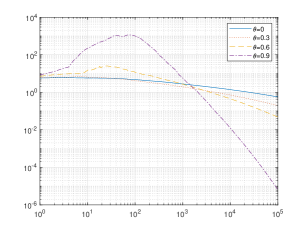
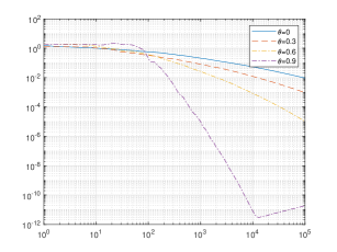
(a) the ssgd method	(b) the prox-RM method

Figure 1: The log-log plot of the stochastic sequence $\{\|v_{k+1}-x^{*}\|\}$ with the same step size but different momentum parameters for least square problem.

The convergence performance is displayed as follows 1. For such a strongly convex function with Lipschitz continuous gradient problem, the nesterov-accelerated ssgd is totally better than the one without, see Figure 1 (a). And the prox-RM is more stable than the ssgd method, where there is no gradient exploding process. Also the convergence performance with nesterov-accelerated prox-RM is better than the one without acceleration, see 1 (b).

6.2 Linear least absolute problem

$A\in\mathbb{R}^{m\times n}$, $b\in\mathbb{R}^{m}$, where $n=100$, $m=10000$, consider the linear least absolute problem $\min\limits_{x}\sum\limits_{k=1}^{m}|a^{\top}_{i}x-b_{i}|$. Then we take the random index on $\{1,\cdots,m\}$ with discrete uniform distribution. Take the random seed 10 of rand in matlab, for example rand(’seed’,10). Take $v$ with $n\times 1$ uniform distribution on $[0,1]$, and $A$ is a standard normal random matrix multiplied by $I+vv^{\top}$. $b=Ax_{0}$, where $x_{0}$ is the optimal. Step size $\alpha_{k}=\frac{1}{2(k+3)^{8/9}}$, momentum parameters $\theta$ are constant .

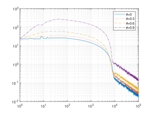
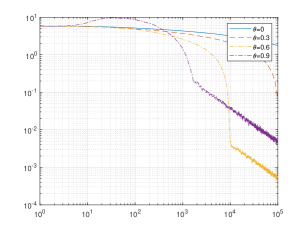
(a) ssgd method	(b) prox-RM method

Figure 2: The log-log plot of the stochastic sequence $\{\|v_{k+1}-x^{*}\|\}$, from stochastic subgradient method with the same step sequence but different momentum parameters for least absolute problem.

The convergence performance is displayed in Figure 2. Although the Nesterov Acceleration method is not better than without the momentum in nonsmooth problem, the almost surely convergence still holds. Also, the prox-RM method is more stable than the ssgd method, where there is no gradient exploding process. Then consider the proximal Robbins-Monro method. Step size $\alpha_{k}=\frac{1}{4(k+3)^{8/9}}$, momentum parameters $\theta$ are constant.

6.3 Composite optimization

Consider the Lasso problem:

$$\min_{x}\frac{1}{n}\sum_{i=1}^{n}(a_{i}^{\top}x-b_{i})^{2}+\|x\|_{1},$$ (6)

where $A\in\mathbb{R}^{m\times n}$, $b\in\mathbb{R}^{m}$, $m=10000$, $n=100$. Take the random seed 10 of rand in matlab, for example rand(’seed’,10). $A$ is a standard normal random matrix and $b$ is a standard normal random vector. Here we only choose the index from $\{1,\cdots,N\}$ randomly and consider the $\|x\|_{1}$ as a certain function. The step-size of gradient and proximal is the same $\alpha_{k}=\frac{1}{20(k+3)^{8/9}}$.

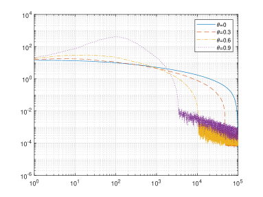
Figure 3: The log-log plot of the stochastic sequence $\{\|v_{k+1}-x_{N}\|\}$, $N=1e5$, different momentum parameters for least absolute problem.

The convergence performance is in Figure 3.

7 Conclusion

This paper introduces a novel framework for analyzing the convergence of stochastic optimization algorithms, particularly those employing Nesterov accelerated methods. The key contributions of the paper are twofold:

1. Supermartingale with delayed information: The paper extends the analysis of stochastic sequences to include delayed term, which is a more realistic representation of the stochastic nature of many optimization problems. By incorporating delayed noise into the expected inequalities, the framework captures the temporal aspect of the stochastic environment, providing a more robust and accurate understanding of the algorithm’s behavior.

2. Nesterov Accelerated Stochastic Approximation: The paper demonstrates the applicability of the framework to the almost sure convergence of Nesterov accelerated stochastic approximation, a powerful optimization technique. This application highlights the practical significance of the theoretical results, as it ensures that the algorithms will converge to a solution with probability one for both stochastic subgradient method and proximal Robbins-Monro method.

In conclusion, the paper offers a novel and comprehensive framework for analyzing the almost sure convergence of Nesterov accelerated methods. These findings contribute to the development of more efficient and reliable optimization techniques, particularly in the context of machine learning, data analysis, and control systems.

References

- [1] Mahmoud Assran and Mike Rabbat. On the convergence of nesterov accelerated gradient method in stochastic settings. In Hal Daum III and Aarti Singh, editors, Proceedings of the 37th International Conference on Machine Learning, volume 119 of Proceedings of Machine Learning Research, pages 410–420. PMLR.
- Benaïm et al. [2005] Michel Benaïm, Josef Hofbauer, and Sylvain Sorin. Stochastic approximations and differential inclusions. SIAM Journal on Control and Optimization, 44(1):328–348, 2005.
- Gitman et al. [2019] Igor Gitman, Hunter Lang, Pengchuan Zhang, and Lin Xiao. Understanding the role of momentum in stochastic gradient methods. In H. Wallach, H. Larochelle, A. Beygelzimer, F. d'Alché-Buc, E. Fox, and R. Garnett, editors, Advances in Neural Information Processing Systems, volume 32. Curran Associates, Inc., 2019.
- Jain et al. [2018] Prateek Jain, Sham M. Kakade, Rahul Kidambi, Praneeth Netrapalli, and Aaron Sidford. Accelerating stochastic gradient descent for least squares regression. In Bubeck Sèbastien, Vianney Perchet, and Philippe Rigollet, editors, Proceedings of the 31st Conference On Learning Theory, volume 75 of Proceedings of Machine Learning Research, pages 545–604. PMLR, 06–09 Jul 2018.
- Kidambi et al. [2018] Rahul Kidambi, Praneeth Netrapalli, Prateek Jain, and Sham Kakade. On the insufficiency of existing momentum schemes for stochastic optimization. In 2018 Information Theory and Applications Workshop (ITA), pages 1–9, 2018.
- Liang et al. [2023] Yuqing Liang, Jinlan Liu, and Dongpo Xu. Stochastic momentum methods for non-convex learning without bounded assumptions. Neural Networks, 165:830–845, 2023.
- Liu and Yuan [2022] Jun Liu and Ye Yuan. On almost sure convergence rates of stochastic gradient methods. In Po-Ling Loh and Maxim Raginsky, editors, Proceedings of Thirty Fifth Conference on Learning Theory, volume 178 of Proceedings of Machine Learning Research, pages 2963–2983, London, UK, 02–05 Jul 2022. PMLR.
- Robbins and Siegmund [1971] H. Robbins and D. Siegmund. A convergence theorem for non negative almost supermartingales and some applications. Optimizing Methods in Statistics, pages 233–257, 1971.
- Robbins and Monro [1951] Herbert Robbins and Sutton Monro. A stochastic approximation method. Annals of Mathematical Statistics, 22(3):400–407, 1951.
- Safavi et al. [2018] Sam Safavi, Bikash Joshi, Guilherme França, and José Bento. An explicit convergence rate for nesterov’s method from sdp. In 2018 IEEE International Symposium on Information Theory (ISIT), pages 1560–1564, 2018.
- Sun et al. [2021] Jianhui Sun, Ying Yang, Guangxu Xun, and Aidong Zhang. A stagewise hyperparameter scheduler to improve generalization. In Proceedings of the 27th ACM SIGKDD Conference on Knowledge Discovery and Data Mining, KDD ’21, pages 1530–1540, New York, NY, USA, 2021. Association for Computing Machinery.
- Sun et al. [2022] Jianhui Sun, Ying Yang, Guangxu Xun, and Aidong Zhang. Scheduling hyperparameters to improve generalization: From centralized sgd to asynchronous sgd. ACM Transactions on Knowledge Discovery from Data, 17:1 – 37, 2022.
- Toulis et al. [2021] Panos Toulis, Thibaut Horel, and Edoardo M. Airoldi. The proximal Robbins-Monro method. Journal of the Royal Statistical Society: Series B (Statistical Methodology), 83:188–212, 2021.
- Wang et al. [2017] Mengdi Wang, Ethan X. Fang, and Han Liu. Stochastic compositional gradient descent: algorithms for minimizing compositions of expected-value functions. Mathematical Programming, 161(1):419–449, 2017.
- Yang [2019] Ethan X. Yang, Mengdi Fang. Multilevel stochastic gradient methods for nested composition optimization. SIAM Journal on Optimization: A Publication of the Society for Industrial and Applied Mathematics, 29(1), 2019.
- Zhou et al. [2020] Kaiwen Zhou, Yanghua Jin, Qinghua Ding, and James Cheng. Amortized nesterov momentum: A robust momentum and its application to deep learning. In Jonas Peters and David Sontag, editors, Proceedings of the 36th Conference on Uncertainty in Artificial Intelligence (UAI), volume 124 of Proceedings of Machine Learning Research, pages 211–220. PMLR, 03–06 Aug 2020.