InfoGaussian: Structure-Aware Dynamic Gaussians through Lightweight Information Shaping

Abstract

3D Gaussians, as a low-level scene representation, typically involve thousands to millions of Gaussians. This makes it difficult to control the scene in ways that reflect the underlying dynamic structure, where the number of independent entities is typically much smaller. In particular, it can be challenging to animate and move objects in the scene, which requires coordination among many Gaussians. To address this issue, we develop a mutual information shaping technique that enforces movement resonance between correlated Gaussians in a motion network. Such correlations can be learned from putative 2D object masks in different views. By approximating the mutual information with the Jacobians of the motions, our method ensures consistent movements of the Gaussians composing different objects under various perturbations. In particular, we develop an efficient contrastive training pipeline with lightweight optimization to shape the motion network, avoiding the need for re-shaping throughout the motion sequence. Notably, our training only touches a small fraction of all Gaussians in the scene yet attains the desired compositional behavior according to the underlying dynamic structure. The proposed technique is evaluated on challenging scenes and demonstrates significant performance improvement in promoting consistent movements and 3D object segmentation while inducing low computation and memory requirements. Our code and trained models will be made available to facilitate future research.

1 Introduction

A real-world scene consists of particles of matter grouped into objects. The motion of an object can be described with each particle moving according to its relationship with other particles when perturbed by an external force. An in-depth explanation of such grouping may resort to quantum mechanics, which describes how the state change of one particle can affect the others. Consequently, we expect that a scene representation could also reflect such a correlation structure to enable efficient inference of object movement for manipulation or interaction. For instance, by simply perturbing a particle from an object, all particles of the object would move simultaneously and consistently.

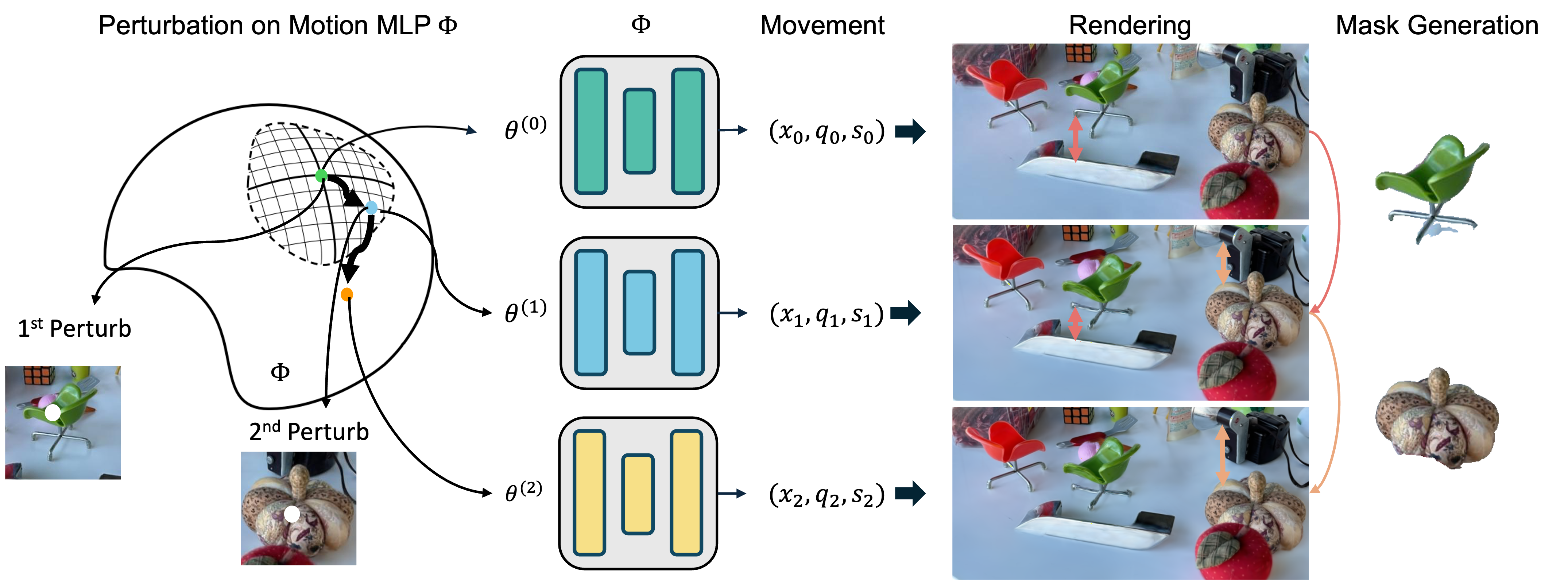
Figure 1: The proposed mutual information shaping of the motion network based on 3D Gaussian Splatting [17] can capture the underlying structure of the scene, while maintaining the correlations after consecutive parameter perturbations. It not only enables moving an object (specified by the arrows) without affecting others by perturbing the network parameters, but also promotes 3D object segmentation by checking the perturbation-induced motion of the Gaussians.

Recently, scene representations have achieved remarkable improvements in terms of rendering quality, e.g., Neural Radiance Fields (NeRFs) [25], and inference efficiency, e.g., 3D Gaussian Splatting (3DGS) [17]. 3DGS reconstructs the scene using a set of 3D Gaussians, similar to a point cloud, by utilizing a point-based rendering framework. To perform object-level tasks, e.g., semantic queries, existing works [6, 51, 45] propose to augment each Gaussian’s parameters by simply adding an extra attribute related to the corresponding task. This strategy could also be applied to model object-level dynamics by specifying each Gaussian’s movement, e.g., spatial coordinates.

However, Gaussians serve as a very low-level scene representation optimized for novel-view synthesis (similar to NeRFs), while the number of objects in the scene is typically much smaller than the number of 3D Gaussians. To synthesize object movement efficiently, we argue that one should leverage the underlying structure of the scene, similar to the quantum binding mentioned above, which is crucial for propagating the changes of one Gaussian to others in resonance, yet is difficult to capture by simply optimizing these low-level representations.

Instead of learning to assign extra attributes to each Gaussian for grouping, we propose a novel and efficient approach to integrate the correlation structure into the scene representation, i.e., directly training a motion network that manipulates Gaussians. Specifically, we use a shared network to generate movements for each Gaussian and enforce correlations among them by biasing the optimization of the network parameters. Eventually, by perturbing the network parameters, the network effectively coordinates among different Gaussians to move coherently, showing reasonable motion trajectories of objects in the scene after rendering. This strategy eliminates the need to estimate and encode pair-wise dynamic correlations among millions of Gaussians, and in contrast, it constructs a well-shaped tangent space capturing the underlying structure of the scene dynamics in a single and simple neural network.

More specifically, we propose a mutual information (MI) shaping technique that encourages correlation among Gaussians from the same object. We leverage the fact that mutual information between the motions of Gaussians can be approximated by the cosine similarity between the Jacobians regarding the perturbed weights. Therefore, we could use the tangent space of the motion network parameters to represent the desired correlation structure. However, shaping the tangent space of the current network does not guarantee that, once perturbed, the perturbed motion network will preserve the well-shaped correlation structure, since changes in its parameters can alter the tangent space, leading to a loss of the desired correlation structure, which is critical to enabling continuously consistent perturbations. Therefore, we prove and propose that, by shaping the activation of the (to be perturbed) set of weights instead of Jacobians, the shaped network can undergo a conformal transformation in the tangent space, ensuring the preservation of the correlation structure and exhibiting consistent motions.

Finally, we develop a pipeline that can efficiently shape a motion network while maintaining consistency in the motion derived from a sequence of perturbations. Our pipeline is fully automated by 2D masks generated from SAM [20]. We evaluate the proposed MI shaping technique in promoting consistent dynamics in various challenging scenes (please see Fig. 1 for examples). To summarize:

• We propose a novel problem of shaping a small motion network in 3DGS to ensure consistent movements under random and continuous perturbations.

• We develop an efficient training pipeline that shapes the motion network only once so that the perturbed network can still synthesize consistent motions without resorting to any reshaping of the tangent space along the motion trajectory.

• We validate that our shaping technique touches only $\sim 7\%$ of all Gaussians during training, while existing methods require optimizing the full parameters of Gaussians. Even though light-weight, our method achieves significant performance improvement in applications like 3D segmentation while significantly reducing computation and memory footprint.

2 Related works

2.1 Scene representations for 3D reconstruction

In recent years, implicit neural representations have emerged as a transformative approach in 3D reconstruction. NeRF [25] is a notable one among the works [2, 10, 16, 23, 24, 49] that parameterize the 3D scene with neural networks. A stream of following works have been proposed to improve under the NeRF framework. Various strategies have been proposed to compress a large-scale 3D scene [15, 26, 33] through introducing a multi-resolution hash table or voxel grids. Leveraging the strengths of explicit modeling, [12, 41, 17] introduces traditional point clouds to model the scene. 3D Gaussian Splatting (3DGS) [17] has been developed to reconstruct 3D scenes with a set of 3D Gaussians for real-time rendering. Applications of these representations includes classical downstream tasks, such as semantic understanding [50, 1, 38, 14, 21], segmentation [13, 45, 6], scene editing  [37, 47, 34, 36, 51, 7], and 3D content creation [35, 8]. While these methods [18, 45] usually assign extra attributes for the related task to each voxel/Gaussian, our work studies how to manipulate the scene based on an underlying scene structure beyond these low-level scene representations. JacobiNeRF [42] has a similar idea to us about correlation shaping on the network, but it aims for label propagation and is a point-wise shaping method that cannot support various scene manipulations.

2.2 Dynamic modeling in 3D scenes

The modeling of dynamic environments constitutes a significant avenue in the 3D domain. Leveraging the capacity of neural fields, D-NeRF [31] promotes NeRF into the dynamic regime by correlating time-varying position offsets with a scene’s canonical space. Follow-up works  [29, 28, 46, 30, 32, 5] proceeds by exploring learning of complex dynamics under the deformable setting. The concept of D-NeRF is further applied within the framework of 3D Gaussian Splatting (3DGS) that adopt a deformable field or extra attributes for 3D Gaussians [44, 39, 11, 43]. Physic-based methods [47, 22, 40] are also introduced into both NeRF and 3DGS framework to generate realistic motion. Diverging from existing methodologies that model the dynamics through simulating each Gaussian’s motion, our research investigates the mutual information shaping of dynamics in a single neural network among scene objects, aiming to generate coherent motion by operating on the network.

3 Modeling mutual information between motions

In this section, we introduce the preliminaries of 3D Gaussian Splatting and our proposed motion representation. We then describe how to achieve consistent movement of Gaussians by Mutual Information shaping in the proposed framework, and how to extend such motion consistency to multi-step cases.

3.1 Dynamics in 3DGS

Given a dataset $\mathcal{D}$ consists of multi-view 2D images and corresponding camera poses, 3D Gaussian Splatting (3DGS) reconstructs the 3D scene by learning a set of 3D Gaussians $\mathcal{G}=\{\mathbf{g}_{1},\mathbf{g}_{2},...,\mathbf{g}_{N}\}$, where $N$ denotes the number of 3D Gaussians in the whole scene. Each 3D Gaussian $\mathbf{g}_{i}$ possesses multiple attributes that can be denoted as $\{\mathbf{x}_{i},\mathbf{s}_{i},\mathbf{q}_{i},\mathbf{o}_{i},\mathbf{c}_{i}\}$. Specifically, $\mathbf{x}_{i}\in\mathbb{R}^{3}$ denotes the location of the centroid of $\mathbf{g}_{i}$, $\mathbf{s}_{i}\in\mathbb{R}^{3}$ denotes the scale, and $\mathbf{q}_{i}\in\mathbb{R}^{4}$ denotes the rotational quaternion, such that $\mathbf{s}_{i}$ and $\mathbf{q}_{i}$ jointly represent the 3D covariance matrix $\mathbf{\Sigma}$ of $\mathbf{g}_{i}$. Furthermore, $\mathbf{o}_{i}\in\mathbb{R}$ denotes the opacity, and $\mathbf{c}_{i}$ denotes the color that is represented as the spherical harmonics(SH) coefficients. Given a camera pose, the color $C(p)$ of a pixel $p$ can be computed by blending a set of depth-ordered Gaussians $\mathcal{N}$ that overlap with $p$:

$$C(p)=\sum_{i\in\mathcal{N}}{\mathbf{c}_{i}\alpha_{i}\prod_{j=1}^{i-1}(1-\alpha_{j})},$$ (1)

where $\mathbf{c}_{i}$ is the color of the $i$-th Gaussian and $\alpha_{i}$ is the blending weight that is calculated with the opacity, projected 2D covariance of the Gaussian, and the location of the pixel.

To model the movement of objects, we hope that we could build a high-level correlation structure in a single motion network for manipulation ease, rather than directly manipulating millions of Gaussians. This network outputs the motion trajectories for each Gaussian, and we can generate a reasonable motion of the object in the scene by simply perturbing the parameters of the network. We borrow the deformation network $\mathbf{\Phi}$ from dynamic modeling in 3D scenes [44, 31] as our motion network. The deformation network is usually is a Multilayer Perceptron (MLP), that maps 3D Gaussians from a canonical space to the time-varying position offsets, generating positional offsets $f(\mathbf{g})$ as follows:

$$f(\mathbf{g})=(\delta\mathbf{x},\delta\mathbf{s},\delta\mathbf{q})=\mathbf{\Phi}(\mathbf{x},\mathbf{t};\theta),$$ (2)

where $(\delta\mathbf{x},\delta\mathbf{s},\delta\mathbf{q})$ are the corresponding offsets of the attributes $(\mathbf{x},\mathbf{q},\mathbf{s})$ at time $\mathbf{t}$, and $\theta$ denotes the parameters of the motion generating MLP $\mathbf{\Phi}$. Further, we let $\mathbf{\Phi}(\mathbf{X},\mathbf{t};\theta)$ be the movements across the entire scene, with $\mathbf{X}$ represents the set positions of all 3D Gaussians.

As we do not need to reconstruct time-varying dynamic scenes, we simplify our motion network that generates positional offsets as $f(\mathbf{g})=\mathbf{\Phi}(\mathbf{X};\theta)$, ablating the variable $\mathbf{t}$.

3.2 Mutual information between motions of 3D Gaussians

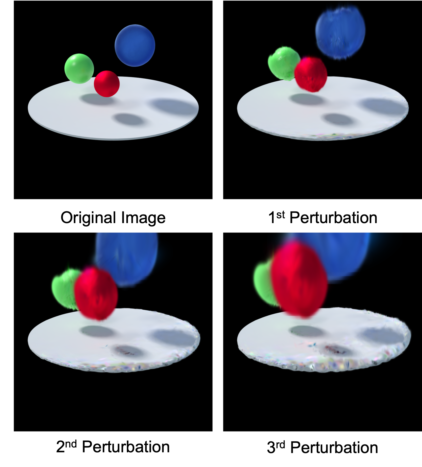
Figure 2: Perturb the deformation network in Deformable 3DGS [44].

We hope that we can directly operate on the motion network to perform the object-level movement. More explicitly, we want to know if an arbitrary change in the parameters of the motion network, $\theta$, can result in reasonable scene motion. To proceed, let $\mathbf{\Phi}(\mathbf{X};\theta)$ be the current movement mapping. and $\mathbf{\Phi}(\mathbf{X};\theta+\mathbf{n})$ represent the corresponding movement after being applied a perturbation $\mathbf{n}$ in the motion representation space. Moreover, if one applies a sequence of perturbations, we can formulate the changes as follows:

$$\mathbf{\Phi}^{(d)}(\mathbf{X};\theta^{(d)})=\mathbf{\Phi}^{(d-1)}(\mathbf{X};\theta^{(d-1)}+\mathbf{n}^{(d)}),d\in\mathbb{N}^{+},$$ (3)

where $\mathbf{\Phi}^{(d)}(\mathbf{X};\theta^{(d)})$ denotes the movement of the scene after the $d$-th perturbation $\mathbf{n}^{(d)}$. Ideally, we expect that the sequence $\{\mathbf{\Phi}^{(d)}(\mathbf{X};\theta^{(d)})\}_{d}$ should exhibit a chain of reasonable movements, depicting an eligible path on the scene manifold.

However, as observed in Fig. 2, a random perturbation in $\theta$ of the original deformable network [44] usually results in unrealistic movements, e.g., two objects might move together without any physical contact. We hypothesize that this phenomena is caused by the lack of mutual correlations among Gaussians.

To characterize the mutual information between motions, we consider two randomly selected 3D Gaussians $\mathbf{g}_{i}$ and $\mathbf{g}_{j}$, and their changed offsets $\hat{f}(\mathbf{g}_{i})$ and $\hat{f}(\mathbf{g}_{j})$ after applying random perturbation $\mathbf{n}$. Following Xu et al. [42], we can show that the mutual information between the motions $\hat{f}(\mathbf{g}_{i})$ and $\hat{f}(\mathbf{g}_{j})$ is proportional to the absolute value of the cosine similarity of the Jacobians of $\mathbf{\Phi}$:

$$\mathbb{I}(\hat{f}(\mathbf{g}_{i}),\hat{f}(\mathbf{g}_{j}))=\log\left(\frac{1}{\sqrt{1-\cos^{2}(\gamma)}}\right)+\text{const.},$$ (4)

where $\gamma$ denotes the angle between the Jacobians $\frac{\partial{\mathbf{\Phi}(\mathbf{x}_{i};\theta)}}{\partial{\theta_{D}}}$ and $\frac{\partial{\mathbf{\Phi}(\mathbf{x}_{j};\theta)}}{\partial{\theta_{D}}}$. Let’s use $\partial{\mathbf{\Phi}}_{i}$ to represent the respective Jacobians for notation clarity.

Accordingly, [42] proposes to enforce the consistency in perturbations by maximizing the quantity in Eq. 4, which is referred to as mutual information shaping of the MLP weights. However, the shaped dynamic scene representation can not ensure consistency once the scene deviates (by perturbation) from the shaped parameters. The underlying reason is that the shaping in [42] is point-wise, e.g., $\partial{\mathbf{\Phi}}_{i}$ and $\partial{\mathbf{\Phi}}_{j}$ can be very similar after shaping in the original tangent space, but there is no guarantee that $\partial{\mathbf{\Phi}}_{i}$ and $\partial{\mathbf{\Phi}}_{j}$ are also similar in the tangent space of perturbed parameter $\theta^{\prime}$. Next, we have a more in-depth discussion and show how we can ensure consistency under consecutive perturbations.

3.3 Motion consistency and compositionality under consecutive perturbations

First, we specify a few terms that we frequently refer to before elaborating on the proposed solution.

Definition 1. Let $\mathcal{G}_{A},\mathcal{G}_{B}\subset\mathcal{G}$ represent two disjoint subsets of the Gaussians, e.g., two objects. We say that the Jacobian $\partial{\mathbf{\Phi}}$ of a motion MLP $\mathbf{\Phi}$ is well-shaped, if and only if, for any two Gaussians $g_{i}\in\mathcal{G}_{A}$ and $g_{j}\in\mathcal{G}_{B}$, there is:

$$\cos(\partial{\mathbf{\Phi}_{i}},\partial{\mathbf{\Phi}_{j}})=\begin{cases}1&\text{if }\mathcal{G}_{A}=\mathcal{G}_{B},\\ 0&\text{if }\mathcal{G}_{A}\neq\mathcal{G}_{B}.\end{cases}$$ (5)

To support generating various object-level motions, we propose that the shaped motion MLP should have: (1) Path Consistency: if the motion MLP $\mathbf{\Phi}$ is well-shaped, the perturbed network $\hat{\mathbf{\Phi}}$ should also be well-shaped, e.g., $\partial\hat{\mathbf{\Phi}}$ satisfies Eq. 5. This condition guarantees that we can perturb $\mathbf{\Phi}$ many times with no need to re-shape. (2) Compositionality: The effect induced by perturbation $\mathbf{n}_{1}+\mathbf{n}_{2}$ should be identical to the combination of the effects induced by $\mathbf{n}_{1}$ and $\mathbf{n}_{1}$ respectively. Next, we introduce two theorems to derive the proposed method, ensuring the above conditions.

Theorem 1. (Path Consistency) Consider perturbing the weights $W^{(l)}$ of the $l$-th linear layer in the network $\mathbf{\Phi}$ (e.g., $\theta_{D}=W^{(l)}$), specified as: $h^{(l)}=W^{(l)}\sigma(h^{(l-1)})+b^{(l)}$. Let $\sigma$ denote the non-linear activation function, $b^{(l)}$ be the bias, and $h^{(l)}$ be the (hidden) output of the $l$-th layer. It is true that if $\partial h^{(l)}$ is well-shaped according to Definition 1 (e.g., $\partial{h}=\frac{\partial h^{(l)}}{\partial W^{(l)}}$ satisfies Eq. 5), $\partial\mathbf{\Phi}$ is also well-shaped. Furthermore, the Jacobian $\partial{\hat{\mathbf{\Phi}}}$ of the perturbed motion network $\partial{\hat{\mathbf{\Phi}}}$ after any number of perturbations, is also well-shaped. We can formulate it as follows:

$$\cos(\partial{\mathbf{\Phi}^{(d)}_{i}},\partial{\mathbf{\Phi}^{(d)}_{j}})\approx\cos(\partial{h^{(0)}_{i}},\partial{h^{(0)}_{j}})=\cos(\partial{\mathbf{\Phi}^{(0)}_{i}},\partial{\mathbf{\Phi}^{(0)}_{j}}),d\in\mathbb{N}^{+},$$ (6)

for arbitrary two Gaussians $g_{i}$ and $g_{j}$. Here $\partial{\mathbf{\Phi}^{(d)}_{i}}$ denotes the Jacobian after the $d$-th perturbation, and $\partial{h^{(0)}_{i}}$ denotes the initial well-shaped Jacobian $\partial h_{i}$ of Gaussian $g_{i}$.

Theorem 2. (Compositionality of Perturbations) Given the above is true, the perturbations through a motion network $\Phi$ should be additive. For instance, given two perturbations $\mathbf{n}_{1}$, $\mathbf{n}_{2}$, we have:

$$\hat{f}(\mathbf{g}_{i}|\mathbf{n}_{1}+\mathbf{n}_{2})\approx\hat{f}(\mathbf{g}_{i}|\mathbf{n}_{1})+\hat{f}(\mathbf{g}_{i},\mathbf{n_{1}}|\mathbf{n}_{2})$$ (7)

The detailed proof of Theorem 1 and $\mathbf{Theorem2}$ can be found in the Appendix. These two theorems imply that we can shape Jacobians $\partial h$ instead of directly shaping $\partial{\mathbf{\Phi}}$. In this case, both Path Consistency and Compositionality can be guaranteed.

4 Mutual information shaping for consistent dynamics

Now we propose InfoGaussian (InfoGS), i.e., Structure-Aware Dynamic Gaussians through Lightweight Information Shaping, following the previous discussion.

4.1 Contrastive learning of MI shaping

According to Eq. 4 and Theorem 1, if we want the movements of two 3D Gaussians to be highly correlated while keeping consistent after perturbations, we can shape their Jacobians $\partial h$ in the motion network $\mathbf{\Phi}$. We first train a plain 3DGS and then train a motion network $\mathbf{\Phi}$ to shape the tangent space.

To shape $\mathbf{\Phi}$ according to Definition 1, we utilize contrastive learning for the shaping. Specifically, we apply the Jensen-Shannon MI estimator (following the formulation in [27]):

$$\mathcal{L}_{MI}=\mathbb{E}_{\mathbb{P}}[-sp(-\cos(\partial{\mathbf{h}_{x}},\partial{\mathbf{h}_{x^{+}}}))]-\mathbb{E}_{\mathbb{P}\times\tilde{\mathbb{P}}}[sp(\cos(\partial{\mathbf{h}_{x}},\partial{\mathbf{h}_{x^{-}}}))]$$ (8)

where $x$ is a sample of the distribution $\mathbb{P}$, $\mathbb{\tilde{P}}=\mathbb{\mathbb{P}}$ is the distribution identical to the empirical probability distribution of the input. $sp(z)=\log(1+e^{z})$ denotes the softplus function. During training, we sample a batch of Gaussians in each epoch to generate positive and negative pairs.

4.2 Coarse mask labeling

Figure 3: The training pipeline of InfoGaussian based on a trained initial 3DGS: (a) We use SAM [20] to generate 2D masks and a pre-trained zero-shot tracker [9] to associate masks from different views. We label the 3D mask of each Gaussian according to the 2D mask of the pixel that owns the Gaussian’s maximal contribution during rendering across all views. (b) We use the labeled 3D masks as the supervision to conduct contrastive learning for mutual information shaping. After shaping, the Jacobians $\partial h$ are consistently distributed in the tangent space.

The key to efficient mutual information shaping via the contrastive learning is how to sample positive and negative pairs among all the 3D Gaussians. It is difficult to know the affiliation of each 3D Gaussian as it requires the knowledge of 3D segmentation. However, leveraging the advance of 2D vision foundation model, we label a coarse mask for each 3D Gaussian by:

$$Mask_{3D}(g_{i})=Mask_{2d}(\mathop{\arg\max}\limits_{p}\,con^{p}_{i})$$ (9)

where $con^{p}_{i}$ represents the contribution of $g_{i}$ to pixel $p$ during rendering. Eq. 9 indicates that the mask of 3D Gaussian $g_{i}$ is determined by the 2D mask of pixel $p$, where the maximal rendering contribution of $g_{i}$ lies in the pixel $p$ across all the given 2D images. We calculate the contribution $con^{p}_{i}$ based on the initial 3D GS. As the initial 3DGS already have the geometric prior of this scene, the mask of Gaussian $g_{i}$ is very likely to be determined by the 2D mask where its maximal contribution manifests.

4.3 Entire shaping pipeline

Fig. 3 illustrates our training pipeline and the training loss can be formulated as:

$$\mathcal{L}=\mathcal{L}_{MI}+\lambda_{r}\mathcal{L}_{reg}+\lambda_{norm}(1.0-\lVert\partial{\mathbf{\Phi}}\rVert)^{2}$$ (10)

where $\mathcal{L}_{MI}$ is the contrastive learning loss given in Eq. 8, $\mathcal{L}_{reg}$ denotes the regularization loss and $\lambda_{r}$ is the corresponding weight. The last term aims to compact the gradients $\partial{\mathbf{\Phi}}$ into a unit sphere so that the perturbation response (scale) of 3D Gaussians from the same object would be similar.

Regularization Loss $\mathcal{L}_{reg}$: To further boost the efficiency, we introduce a natural regularization in the self-supervised training. Since an object is continuous in space, the neighboring Gaussians of $\mathbf{g}_{i}$ should be very likely to belong to the same object as $\mathbf{g}_{i}$. This observation could help shape the Jacobians of 3D Gaussians inside the object that are heavily occluded by other Gaussians, as they may not receive the accurate annotation in the coarse 3D segmentation. Thus, these Gaussians could be supervised by the nearby well-labeled Gaussians. Specifically, $\mathcal{L}_{reg}$ is formulated as:

$$\mathcal{L}_{reg}=\mathbb{E}_{\mathbb{P}}[\frac{1}{k}\sum_{x^{+}\in n(x)}1.0-\cos(\mathbf{\Phi}_{x},\mathbf{\Phi}_{x^{+}})]$$ (11)

where $\mathbb{P}$ denotes the input space, $n(x)$ denotes the neighboring Gaussians of $x$, and $k=\lVert n(x)\rVert$ is the number of neighbors. In practice, the distance between two Gaussians is defined by the Euclidean distance of their centroid $\mathbf{x}$, and $k$ is a fixed hyper-parameter during the training.

5 Experiments

5.1 Implementation details

Training. We shape the motion MLP $\mathbf{\Phi}$ based on a trained initial 3D Gaussian Splatting. Specifically, we first train a plain 3D Gaussian cloud following the original 3DGS pipeline, to learn the canonical space of a static scene. Second, we follow the shaping pipeline in Sec. 4.3 to shape $\mathbf{\Phi}$. All experiments are conducted on a single RTX 3090 GPU for only 20 seconds (excluding the time cost for training plain 3D GS). Detailed hyper-parameter settings can be found in the Appendix.

Datasets. As we focus on generating the path from a single point on the scene manifold (i.e., the scene of a certain time step), we utilize open-world static datasets LERF-Localization [18] and Mip-NeRf360 [3], in order to evaluate the consistent dynamics modeling in more complex and compositional scenarios. We also test it on the real dynamic and compositional (i.e., multi-objects) scenes in D-NeRF dataset [31]; Regarding downstream application like 3D segmentation, We provide benchmark results on the LERF-Mask dataset [45], where test views have accurate mask annotation.

Baselines. For dynamics evaluation, we utilize the MI shaping method in JacobiNeRF [42] as a substitute for our MI shaping $\mathcal{L}_{MI}$ in 4.3, which is a point-wise method for shaping the network in response to individual perturbations. While keeping other loss terms the same, we name this baseline JaocbiGS. For 3D segmentation, besides JacobiGS, we adopt two more baselines: LERF[18] and Gaussian Grouping[45] that do not use MI shaping to achieve segmentation. These methods assign an extra feature for each volume or 3D Gaussian to predict the 2D mask through projection.

5.2 Consistent dynamics modeling

Task Setting. To validate the effectiveness of mutual information shaping for consistent dynamics, we perturb the motion MLP using the Jacobians of Gaussians $\partial\mathbf{\Phi}$ and examine the perturbation’s effects on the generated images. Specifically, for a certain test image $I_{t}$ and its camera pose $v_{t}$, we simulate the human clicking by selecting a pixel $p_{t}$ in $I_{t}$. We select the Gaussian $g_{t}$ that contributes the most to the current pixel prompt when rendering (similar to Coarse Mask Labeling in Sec. 4.2). We then use the Jacobian $\partial\mathbf{\Phi}_{t}=\frac{\partial\mathbf{\Phi}(\mathbf{x}_{t})}{\partial W^{(l)}}$ to perturb $W^{(l)}$, the weight matrix of the $l$-th layer. To generate new scenes under camera pose $v_{t}$ for each perturbation, we add the difference $\hat{f}(\mathcal{G})-f(\mathcal{G})$ in the movement to the corresponding parameters $(\mathbf{x},\mathbf{q},\mathbf{s})$, and rerender the scene.

5.2.1 Qualitative results

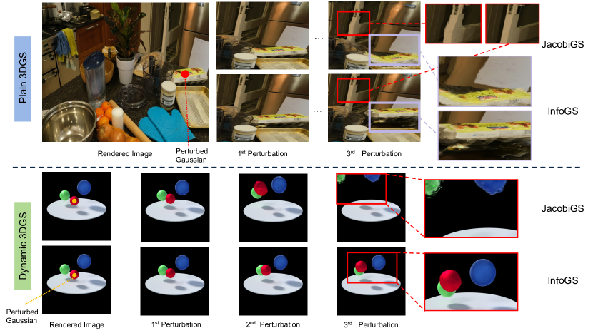
Figure 4: Qualitative comparison for consecutive perturbations in static and dynamic scenarios.

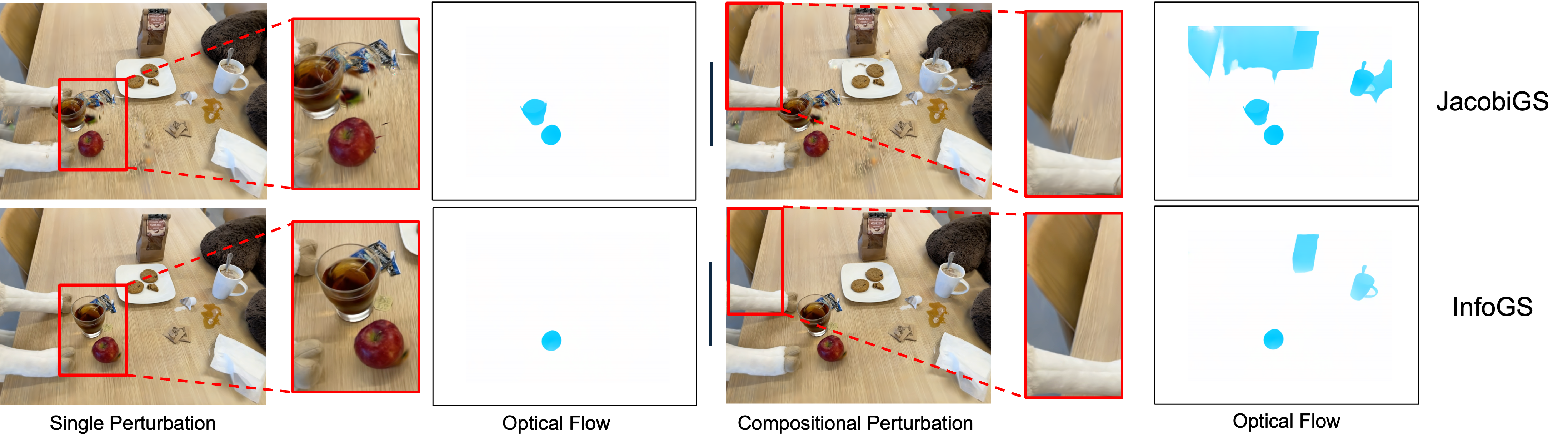
Figure 5: Qualitative comparison for compositional perturbations.

For path consistency, as shown in Fig. 4, perturbing each scene with the same pixel prompt reveals that InfoGS induces reasonable motion (e.g., the box of eggs is lifted up) while preserving the uncorrelated objects. It exhibits path-consistent motion, satisfying path consistency in successive perturbations. In contrast, scenes generated by JacobiGS diverge into unrealistic representations after the second and third perturbation. For example, consecutive perturbations to the box of eggs results in the distortion of the door behind the box (see the red box comparison of the upper part in Fig. 4). An ablation study of the impact of MI shaping on deformable 3DGS can be found in the appendix.

Regarding compositionality, as shown in Fig. 5, JacobiGS has difficulty maintaining scene integrity when combining Jacobians of two or more objects for perturbations. For instance, the table nearby is also affected by the perturbation (see the red box comparison of the right part in Fig. 5). Conversely, InfoGS effectively maintains robust correlation shaping, demonstrating superior performance in preserving the scene under composite perturbations.

The observations from Fig. 4 and Fig. 5 demonstrate that InfoGaussian supports diverse and consecutive perturbations, thereby facilitating the generation of realistic new scenes. This effectively corroborates the principles outlined in Theorem 1 and Theorem 2.

5.2.2 Quantitative results

Table 1: Quantitative results of consistent dynamic

Type	Model	LERF-Mask	MipNeRF-360
		LPIPS	LPIPS
Path Consistency	JacobiGS w/o CML  [42]	0.385	0.388
	JacobiGS w/ CML  [42]	0.371	0.366
	InfoGS	0.164	0.183
Compositionality	JacobiGS w/o CML  [42]	0.537	0.562
	JacobiGS w/ CML  [42]	0.452	0.463
	InfoGS	0.213	0.217

We quantitatively evaluate our proposed method by measuring rendered image quality after various perturbations. Specifically, we compare the rendered image after consecutive or compositional perturbations shown in Fig. 4,5 with the unperturbed image to calculate the LPIPS score [48]. This metric computes the perceptual similarity between the unperturbed and perturbed images.

From Tab. 1, we can see that our method has better image quality after various perturbation, indicating the naturalness of the generated motion. Furthermore, original JacobiNeRF shaping is totally supervised by 2D through projection, so here we ablate the coarse mask labeling from JacobiGS and follow the supervision in JaobiNeRF, we find that the performance deteriorates, further demonstrating the effectiveness of 3D supervision supported by coarse mask labeling.

5.3 3D segmentation

Task Setting. By discovering the motion correlations among Gaussians, our approach enables 3D segmentation through perturbation techniques. This is predicated on the observation that Gaussians exhibiting similar motion patterns are likely associated with the same object. Specifically, given a point prompt or mask prompt of an object for test view $v_{t}$, we perturb the scene through the methodology detailed in Sec. 5.2. Using the average gradient of the selected Gaussians to perturb the motion MLP, we classify the group of Gaussians demonstrating significant motion as a single object.

Figure 6: Upper: Qualitative results of Open Vocabulary Segmentation [45]. Lower: The relevance map when perturbing a single Gaussian (highlighted by the white ellipse in the purple circle)

5.3.1 Results and analysis

Table 2: Quantitative results of Open Vacabulary Segmentation on LERF-Mask dataset. The time and memory costs mentioned refer to the total consumption minus the resources used for the initial training of the Gaussian. Therefore, direct comparisons with LERF in this table are not feasible.

Model	figurines		ramen		teatime		Average Training Cost
	mIoU	mBIoU	mIoU	mBIoU	mIoU	mBIoU	Time/Minutes	Memory/M	#GS Used
LERF [18]	33.5	30.6	28.3	14.7	49.7	42.6	*	*	*
JacobiGS [42]	62.2	60.1	64.3	57.7	69.7	70.1	10.2	3.3	17%
Gaussian Grouping [45]	69.7	67.9	77.0	68.7	71.7	66.1	48.2	688.2	100%
InfoGS	80.6	77.2	80.6	70.1	84.5	78.7	0.3	3.3	7%

For quantitative results, Tab. 2 demonstrates that InfoGS significantly outperforms than both NeRF-based and GS-based methods. Compared with previous state-of-the-art results, InfoGS increases the mIoU by average $11\%$. Additionally, it also exhibits better performance in the boundary metric mBIoU. Though the segmentation can be done in a single perturbation, JacobiGS still performs worse than InfoGS, indicating Jacobian $\partial h$ can be easier and better shaped than $\partial\mathbf{\Phi}$.

Qualitative results are shown in Fig. 6. We could see that InfoGS produces sharp boundaries for the segmentation without any blurs. We also provide the relevance map when perturbing a single Gaussian to select the object. The relevance scores are represented as the cosine similarities of the Jacobians $\partial\mathbf{\Phi}$ of the perturbed Gaussian and all other Gaussians. As illustrated in Fig. 6, when perturbing a single Gaussian, the object it belongs to is highlighted, explaining InfoGS’s great ability of segmentation from another perspective. And it also shows that the relevance of Jacobian would be higher if a Gaussian is closer to the perturbed one (see (b) in Fig. 6. This phenomena obeys our real-world observations, indicating the flexibility of MI shaping for simulating the real-world physics.

The superior performance of our methods could be attributed to the awareness of scene structure. Instead of directly assigning structuring attributes to each Gaussian [6, 51, 45], we focus on shaping a network that acts on the Gaussians in a way that expresses the desired structure. It helps a lot for the low-level representation like 3DGS when performing on the high-level tasks like segmentation. The shaped MLP is aware of the entire scene structure rather than a single Gaussian. Notably, we only sample about $7\%$ of all the Gaussians during training for convergence, boosting the training time by $100$x with only $0.5\%$ memory storage compared to previous methods (see Tab. 2).

6 Discussion

We investigate the problem of shaping a motion network to capture the correlation structure in the scene based on a 3DGS model to encourage consistent object-level dynamics under random scene perturbations in a highly efficient way. Our derivation shows that enforcing the Jacobians of the output of an intermediate linear layer can ensure the consistency of the entire motion network even after continuous perturbations. We demonstrate the effectiveness of the proposed using an efficient training pipeline composed of a contrastive loss and a sampling strategy for correlated 3D Gaussians with pre-trained foundation models. The shaped motion network not only allows consistent movements but also induces quality 3D segmentation masks. Despite the efficiency, the controllability of our current pipeline to synthesize arbitrarily complex motions is limited. We would like to resolve the limitation by learning dynamics from a large-scale video dataset in future work.

Appendix A Implementation details

A.1 Model architecture

As shown in Fig. 7, the motion network $\mathbf{\Phi}$, instantiated as a 4-layer MLP with ReLU activation, maps the coordinates $\mathbf{x}$ of each Gaussian in the canonical space to its displacement $(\delta\mathbf{x},\delta\mathbf{s},\delta\mathbf{q})$. Following the setting of the deformation network [44], the mapping can be written as follows:

$$(\delta\mathbf{x},\delta\mathbf{s},\delta\mathbf{q})=\mathbf{\Phi}(\kappa(\text{sg}(\mathbf{x})),$$ (12)

where $\text{sg}(\cdot)$ denotes a stop-gradient operation, $\kappa$ denotes the positional encoding:

$$\kappa(p)=(\sin(2^{k}\pi p,\cos(2^{k}\pi p))^{L-1}_{k=0},$$ (13)

where $L=10$ during our experiments to represent higher frequency functions. We first transform the input coordinates in the canonical space $\gamma(x)$ with a positional encoding. Then, the positional encoding of the input location is passed through 4 fully-connected linear layers with ReLU activation, each with 512 channels. Then a final linear layer (without activation) outputs the displacement $(\delta\mathbf{x},\delta\mathbf{s},\delta\mathbf{q})$.

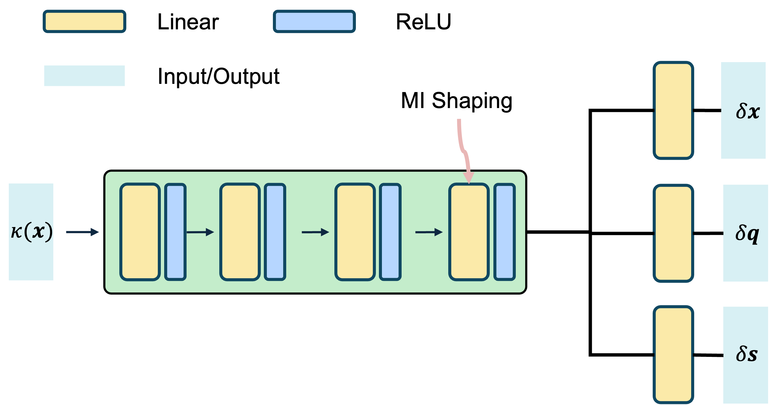
Figure 7: The architecture of motion network.

A.2 Training details

During training, we set the hyperparameters $\lambda_{r}=0.1$ and $\lambda_{norm}=1.0$. We adopt the Adam optimizer [19] when shaping the motion network, with a learning rate of $0.001$. The gradient that we use to shape the motion network is $\partial h=\frac{\partial h^{(l)}}{\partial W^{(l)}}$ with $l=4$, namely, the weight of the linear layer before the final output layer. We train the network for $400$ iterations and sample a batch of $512$ 3D Gaussians at each iteration to compute the training loss.

Appendix B Theorem proof

B.1 Proof of theorem 1

Theorem 1. (Path Consistency) Consider perturbing the weights $W^{(l)}$ of the $l$-th linear layer in the network $\mathbf{\Phi}$ (e.g., $\theta_{D}=W^{(l)}$), specified as: $h^{(l)}=W^{(l)}\sigma(h^{(l-1)})+b^{(l)}$. Let $\sigma$ denote the non-linear activation function, $b^{(l)}$ be the bias, and $h^{(l)}$ be the (hidden) output of the $l$-th layer. It is true that if $\partial h^{(l)}$ is well-shaped according to Definition 1 (e.g., $\partial{h}=\frac{\partial h^{(l)}}{\partial W^{(l)}}$ satisfies Eq. 5), $\partial\mathbf{\Phi}$ is also well-shaped. Furthermore, the Jacobian $\partial{\hat{\mathbf{\Phi}}}$ of the perturbed motion network $\partial{\hat{\mathbf{\Phi}}}$ after any number of perturbations, is also well-shaped. We can formulate it as follows:

$$\cos(\partial{\mathbf{\Phi}^{(d)}_{i}},\partial{\mathbf{\Phi}^{(d)}_{j}})\approx\cos(\partial{h^{(0)}_{i}},\partial{h^{(0)}_{j}})=\cos(\partial{\mathbf{\Phi}^{(0)}_{i}},\partial{\mathbf{\Phi}^{(0)}_{j}}),d\in\mathbb{N}^{+},$$ (14)

for two Gaussians $g_{i}$ and $g_{j}$. Here $\partial{\mathbf{\Phi}^{(d)}_{i}}$ denotes the Jacobian after the $d$-th perturbation, and $\partial{h^{(0)}_{i}}$ denotes the well-shaped Jacobian $\partial h_{i}$ of $g_{i}$.

To illustrate Theorem 1, we need to factorize the gradient of Gaussian $g_{i}$:$\partial\mathbf{\Phi}_{i}=\frac{\partial{\mathbf{\Phi}(\mathbf{x}_{i};\theta)}}{\partial{\theta_{D}}}$, to reveal its relationship with the perturbed weight $W^{(l)}$. With out loss of generality, we consider the relationship between an arbitrary scalar $z$ in the output $(\delta\mathbf{x},\delta\mathbf{s},\delta\mathbf{q})$ of motion network and perturbed weight $W^{(l)}$:

$$z=Y(h^{(l)})=Y(W^{(l)}\sigma(h^{(l-1)})+b^{(l)}),$$ (15)

where $Y$ denotes all the transformations after $l$-th layer, $z$ denotes an arbitrary scalar in the vector output of $\mathbf{\Phi}$. Then the differential $\mathrm{d}{z}$ could be written as:

$$\mathrm{d}{z} =\frac{\partial z}{\partial h^{(l)}}^{\top}\mathrm{d}{h^{(l)}}=\sigma(h^{(l-1)})\frac{\partial z}{\partial h^{(l)}}^{\top}\mathrm{d}{W^{(l)}}$$ (16)

$$=\text{tr}(\sigma(h^{(l-1)})\frac{\partial z}{\partial h^{(l)}}^{\top}\mathrm{d}{W^{(l)}}),$$

as $\mathrm{d}{z}=\text{tr}(\frac{\partial z}{\partial W^{(l)}}^{\top}\mathrm{d}{W^{(l)}})$, we could get that:

$$\frac{\partial z}{\partial W^{(l)}}=\frac{\partial z}{\partial h^{(l)}}\sigma(h^{(l-1)})^{\top},$$ (17)

which is a 2D matrix that has the same shape with the $W^{(l)}$. Then the cosine similarity of Jacobians $\partial\mathbf{\Phi}$ between two Gaussians are:

$$\cos(\partial\mathbf{\Phi}_{i},\partial{\mathbf{\Phi}}_{j}) =\frac{(\frac{\partial z(\mathbf{x}_{i})}{\partial h^{(l)}(\mathbf{x}_{i})}\sigma(h^{(l-1)}(\mathbf{x}_{i}))^{\top})\cdot(\frac{\partial z(\mathbf{x}_{j})}{\partial h^{(l)}(\mathbf{x}_{j})}\sigma(h^{(l-1)}(\mathbf{x}_{j}))^{\top})}{\lVert\partial\mathbf{\Phi}_{i}\rVert\lVert\partial\mathbf{\Phi}_{j}\rVert}$$ (18)

$$=\frac{(\frac{\partial z(\mathbf{x}_{i})}{\partial h^{(l)}(\mathbf{x}_{i})}\cdot\frac{\partial z(\mathbf{x}_{j})}{\partial h^{(l)}(\mathbf{x}_{j})})(\sigma(h^{(l-1)}(\mathbf{x}_{i}))^{\top}\cdot\sigma(h^{(l-1)}(\mathbf{x}_{j}))^{\top})}{\lVert\partial\mathbf{\Phi}_{i}\rVert\lVert\partial\mathbf{\Phi}_{j}\rVert},$$

because $\partial h=\frac{\partial h^{(l)}}{\partial W^{(l)}}$ could be formulated as a 3D tensor, which could be conceptualized as a collection of gradients and each gradient is the vector $\sigma(h^{(l-1)})$. If $\partial h$ is well-shaped satisfying Eq. 5, then $\sigma(h^{(l-1)})$ should also satisfy 5. In this case, if $g_{i}$ and $g_{j}$ are affiliated to different objects:

$$\cos(\partial\mathbf{\Phi}_{i},\partial{\mathbf{\Phi}}_{j}) =\frac{(\frac{\partial z(\mathbf{x}_{i})}{\partial h^{(l)}(\mathbf{x}_{i})}\cdot\frac{\partial z(\mathbf{x}_{j})}{\partial h^{(l)}(\mathbf{x}_{j})})(\sigma(h^{(l-1)}(\mathbf{x}_{i}))^{\top}\cdot\sigma(h^{(l-1)}(\mathbf{x}_{j}))^{\top})}{\lVert\partial\mathbf{\Phi}_{i}\rVert\lVert\partial\mathbf{\Phi}_{j}\rVert}$$ (19)

$$=\frac{(\frac{\partial z(\mathbf{x}_{i})}{\partial h^{(l)}(\mathbf{x}_{i})}\cdot\frac{\partial z(\mathbf{x}_{j})}{\partial h^{(l)}(\mathbf{x}_{j})})(0)}{\lVert\partial\mathbf{\Phi}_{i}\rVert\lVert\partial\mathbf{\Phi}_{j}\rVert}$$

$$=0,$$

Eq. 19 indicates that if $\cos(\partial h_{i},\partial h_{j})=0$ when $g_{i}$ and $g_{j}$ are affiliated to different objects (e.g. $\mathcal{G}_{A}\neq\mathcal{G}_{B}$ in Eq. 5), then $\cos(\partial\mathbf{\Phi}_{i},\partial{\mathbf{\Phi}}_{j})=0$. Meanwhile, $\sigma(h^{(l-1)})$ would not change since it is the input of the perturbed layer $l$ and the input of $\mathbf{\Phi}$ is the fixed $\mathbf{x}$ from the canonical space, then $\cos(\partial h_{i},\partial h_{j})=0$ would be consistent during the perturbation. Therefore, we could prove the following lemma: Lemma 1. (Orthogonality) After any number of perturbations, the orthogonality of Jacobians between two Gaussians $g_{i}\in\mathcal{G}_{A}$ and $g_{j}\in\mathcal{G}_{B}$ that are affiliated to different objects ($\mathcal{G}_{A}\neq\mathcal{G}_{B}$) would remain consistent:

$$\cos(\partial{\mathbf{\Phi}^{(d)}_{i}},\partial{\mathbf{\Phi}^{(d)}_{j}})=\cos(\partial{h^{(d)}_{i}},\partial{h^{(d)}_{j}})=\cos(\partial{h^{(0)}_{i}},\partial{h^{(0)}_{j}}),d\in\mathbb{N}^{+},$$ (20)

In contrast, we have another lemma: Lemma 2. (Similarity) After any number of perturbations, the similarity of Jacobians between two Gaussians $g_{i}\in\mathcal{G}_{A}$ and $g_{j}\in\mathcal{G}_{B}$ that are affiliated to the same objects ($\mathcal{G}_{A}=\mathcal{G}_{B}$) would remain consistent:

$$\cos(\partial{\mathbf{\Phi}^{(d)}_{i}},\partial{\mathbf{\Phi}^{(d)}_{j}})\approx\cos(\partial{h^{(d)}_{i}},\partial{h^{(d)}_{j}})=\cos(\partial{h^{(0)}_{i}},\partial{h^{(0)}_{j}}),d\in\mathbb{N}^{+},$$ (21)

Proof: Consider the set of Jacobians $J_{A}=\{\partial\mathbf{\Phi}_{i},g_{i}\in\mathcal{G}_{A}\}$ of all Gaussians in an arbitrary object $\mathcal{G}_{A}$, they all would be orthogonal to the Jacobians of Gaussians from other objects, according to Lemma 1 if the unperturbed motion network $\mathbf{\Phi}$ is well-shaped. Thus, the representation space of $J_{A}$ would be very narrow. If the representation space of $\partial\mathbf{\Phi}$ is compact enough (e.g., the dimension of the representation space of $\partial\mathbf{\Phi}$ is identical to the number of objects in the scene), $\cos(\partial{\mathbf{\Phi}^{(d)}_{i}},\partial{\mathbf{\Phi}^{(d)}_{j}})=1$ when $\mathcal{G}_{A}=\mathcal{G}_{B}$. In this extreme case, the set of Jacobians from all the objects in the scene is a group of canonical basis [4] of the representation space of $\partial\mathbf{\Phi}$.

Combining Lemma 1 and Lemma 2, we could have the conclusion in $\mathbf{Theorem1}$.

B.2 Proof of theorem 2

Theorem 2. (Compositionality of Perturbations) Given the above is true, the perturbations through a motion network $\mathbf{\Phi}$ should be additive. For instance, given two different perturbations $\mathbf{n}_{1}$, $\mathbf{n}_{2}$, we have:

$$\hat{f}(\mathbf{g}_{i}|\mathbf{n}_{1}+\mathbf{n}_{2})\approx\hat{f}(\mathbf{g}_{i}|\mathbf{n}_{1})+\hat{f}(\mathbf{g}_{i},\mathbf{n_{1}}|\mathbf{n}_{2})$$ (22)

To prove $\mathbf{Theorem2}$, we could first expand the left term:

$$\hat{f}(\mathbf{g}_{i}|\mathbf{n}_{1}+\mathbf{n}_{2}) =\mathbf{\Phi}(\mathbf{x}_{i};\theta+(\mathbf{n}_{1}+\mathbf{n}_{2}))-\mathbf{\Phi}(\mathbf{x}_{i};\theta)$$ (23)

$$\approx\mathbf{\Phi}(\mathbf{x}_{i};\theta)+(\mathbf{n}_{1}+\mathbf{n}_{2})\cdot\frac{\partial\mathbf{\Phi}(\mathbf{x}_{i};\theta)}{\partial\theta}-\mathbf{\Phi}(\mathbf{x}_{i};\theta)$$

$$=\mathbf{n}_{1}\cdot\frac{\partial\mathbf{\Phi}(\mathbf{x}_{i};\theta)}{\partial\theta}+\mathbf{n}_{2}\cdot\frac{\partial\mathbf{\Phi}(\mathbf{x}_{i};\theta)}{\partial\theta}$$

using Taylor-expansion. Similarly, we can expand the right term:

$$\hat{f}(\mathbf{g}_{i}|\mathbf{n}_{1})+\hat{f}(\mathbf{g}_{i},\mathbf{n_{1}}|\mathbf{n}_{2}) \approx\mathbf{n}_{1}\cdot\frac{\partial\mathbf{\Phi}(\mathbf{x}_{i};\theta)}{\partial\theta}+\mathbf{n}_{2}\cdot\frac{\partial\mathbf{\Phi}(\mathbf{x}_{i};(\theta+\mathbf{n}_{1}))}{\partial(\theta+\mathbf{n}_{1})}$$ (24)

consider perturbing an arbitrary object in the second perturbation that is different from $\mathbf{n}_{1}$, namely $\mathbf{n}_{2}=\partial\mathbf{\Phi}_{q}$, the $\partial\mathbf{\Phi}_{q}$ is the Jacobians of Gaussian $g_{q}$ affiliated to an arbitrary object, except the one that $\mathbf{n_{1}}$ is perturbing. Then Eq. 22 and Eq. 24 could be reformulated as:

$$\hat{f}(\mathbf{g}_{i}|\mathbf{n}_{1}+\mathbf{n}_{2}) \approx\mathbf{n}_{1}\cdot\frac{\partial\mathbf{\Phi}(\mathbf{x}_{i};\theta)}{\partial\theta}+\frac{\partial\mathbf{\Phi}(\mathbf{x}_{q};\theta)}{\partial\theta}\cdot\frac{\partial\mathbf{\Phi}(\mathbf{x}_{i};\theta)}{\partial\theta},$$ (25)

$$\hat{f}(\mathbf{g}_{i}|\mathbf{n}_{1})+\hat{f}(\mathbf{g}_{i},\mathbf{n_{1}}|\mathbf{n}_{2}) \approx\mathbf{n}_{1}\cdot\frac{\partial\mathbf{\Phi}(\mathbf{x}_{i};\theta)}{\partial\theta}+\frac{\partial\mathbf{\Phi}(\mathbf{x}_{q};(\theta+\mathbf{n}_{1}))}{\partial(\theta+\mathbf{n}_{1})}\cdot\frac{\partial\mathbf{\Phi}(\mathbf{x}_{i};(\theta+\mathbf{n}_{1}))}{\partial(\theta+\mathbf{n}_{1})},$$ (26)

and $x_{q}$ and $x_{i}$ are affiliated to different objects, then $\frac{\partial\mathbf{\Phi}(\mathbf{x}_{q};\theta)}{\partial\theta}\cdot\frac{\partial\mathbf{\Phi}(\mathbf{x}_{i};\theta)}{\partial\theta}=\frac{\partial\mathbf{\Phi}(\mathbf{x}_{q};(\theta+\mathbf{n}_{1}))}{\partial(\theta+\mathbf{n}_{1})}\cdot\frac{\partial\mathbf{\Phi}(\mathbf{x}_{i};(\theta+\mathbf{n}_{1}))}{\partial(\theta+\mathbf{n}_{1})}=0$ according to Theorem 1, as the orthogonality preserves during the perturbation. Therefore, we could get:

$$\hat{f}(\mathbf{g}_{i}|\mathbf{n}_{1}+\mathbf{n}_{2})\approx\mathbf{n}_{1}\cdot\frac{\partial\mathbf{\Phi}(\mathbf{x}_{i};\theta)}{\partial\theta}\approx\hat{f}(\mathbf{g}_{i}|\mathbf{n}_{1})+\hat{f}(\mathbf{g}_{i},\mathbf{n_{1}}|\mathbf{n}_{2}),$$ (27)

the above equation points out that perturbations to different objects would not affect each other if the motion network $\mathbf{\Phi}$ is well-shaped.

Appendix C Additional experimental results

C.1 Ablation Study

C.1.1 Impact of shaping on the deformable 3DGS

Table 3: Imapact of InfoGS on the Deformable 3DGS [44] in D-NeRF datasets [31]

Model	PSNR$\uparrow$	SSIM$\uparrow$	LPIPS$\downarrow$
w/o InfoGS	41.0	0.995	0.009
w/ InfoGS	39.7	0.993	0.012

The training loss introduced in Eq. 10 can be integrated to the deformation network in Deformable 3D Gaussian Splatting [44], as our motion framework has a similar structure to the deformation network. We reformulate the training loss as:

$$\mathcal{L}=\mathcal{L}_{img}+\lambda\mathcal{L}_{infogs},$$ (28)

where the $\mathcal{L}_{img}$ indicates the training loss in the original framework that produces time-varying positional offsets for each Gaussian and renders the scene, supervised from the images from each time step. And the $\mathcal{L}_{infogs}$ is the training loss introduced in our framework, specified in Eq. 10. $\lambda$ is the weight, and we set it to $0.1$.

During training, we first solely complete the training process in the original framework, and fine-tune the deformation network by adopting the loss in Eq. 28. At each time step, we follow the training pipeline in InfoGS, sampling $512$ Gaussians in the scene to calculate the $\mathcal{L}_{infogs}$ loss.

The result is shown in Tab. 3. We can see that our shaping technique does leading a small performance drop in memorizing the motion trajectories given in the dynamics dataset. But this sacrifice has allowed us to perturb the deformation network from arbitrary time steps and generate reasonable motion shown in Fig. 4. What’s more, the deformation network aims to reconstruct the dynamic scene rather than generate consistent motion. Therefore, the drop in reconstruction performance when introducing an extra loss that aims for motion generation is reasonable.

C.1.2 Impact of regularization loss

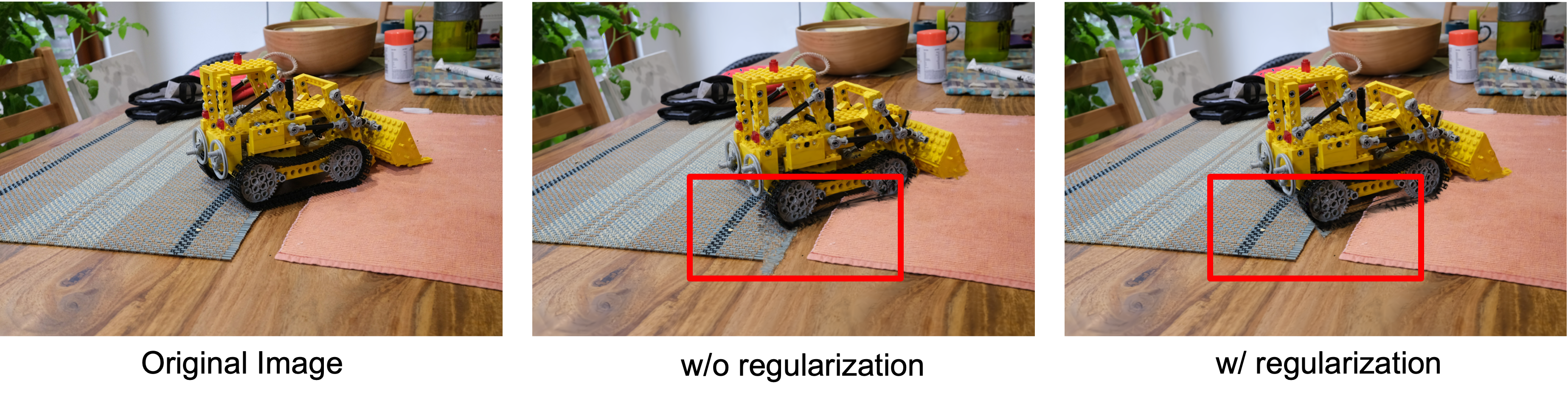
Figure 8: The impact of regularization loss when perturbing the lego tractor.

We introduce an extra regularization loss to help shape the Jacobians. Here Fig. 8 shows the ablation study of this regularization loss. From the area, the area in the red box apparently illustrates the impact of the regularization loss. When perturbing a Gaussian of the tractor, the one with regularization loss can maintains the minimal affects to other objects, while the one without it produces some artifacts to the surroundings. It demonstrates that the regularization loss can better shape the correlation structure of the tangent space of the motion network.

C.2 Sparse representations

We then further explore the property of the representation space of shaped Jacobians $\partial\mathbf{\Phi}$. When perturbing an object using random noise $\mathbf{n}$, the previous MI shaping framework [42] directly uses the Jacobian that is related to this object. In specific, when applying it in 3DGS, $\mathbf{n}=\lambda_{s}\partial\mathbf{\Phi}_{i}$ where $g_{i}$ is one of the Gaussians of this object and $\lambda_{s}$ is a scaling factor. In the experiments of our work, we also follow the same way to perturb the objects, ensuring that other objects are not perturbed by the orthogonality (see Lemma 1).

The representation space of motion would be very narrow if we could only use a similar Jacobian to perturb the object. This is because the Jacobians of the same object would be very similar due to MI shaping (in practice, the Jacobians of Gaussians of the same object could be shaped to nearly identical). However, we expect that we could have various ways to perturb an object without affecting any other objects. To achieve this, the Jacobians of an object need to lie in an independent subspace of the whole representation space. Namely, this subspace needs to be disjoint with the subspaces of Jacobians of other objects. To verify, we randomly select a Gaussian $g_{i}$ and consider the indices of non-zero values in $\partial\mathbf{\Phi}_{i}$ as the subspace of the object $g_{i}$ belongs to. We randomly use a unit vector in this subspace to create a plane with $\partial\mathbf{\Phi}_{i}$, then we get a 2D plane in this subspace. Finally, we twist $\partial\mathbf{\Phi}_{i}$ by different degrees within this 2D plane and use the changed Jacobian to perturb the object each time we twist.

Figure 9: Circular motion in the representation subspace of the Jacobians of an object (twist the Jacobian by different degrees in the subspace). The perturbed object in this Blender synthetic scene [25] behaves in a periodic motion. We only preserve the change of centroid $\mathbf{x}$ to show a clear motion trace.

Fig. 9 shows the generated scenes when we twist the Jacobian in a circular motion. We can see that the silver object also periodically moves. Especially, when we twist the Jacobian by $90\degree,270\degree$, the scene remains static, as the twisted Jacobian is perpendicular to the original one. When the Jacobian is rotating, other objects do not receive any perturbations. It indicates that the Jacobians of an object indeed lie in an independent subspace and we could manipulate the perturbed noise $\mathbf{n}$ within the subspace.

What’s more, because we consider the indices of non-zero values in $\partial\mathbf{\Phi}_{i}$ as the subspace of the object $g_{i}$ belongs to, Fig. 9 further demonstrates the sparsity of the shaped Jacobians in InfoGaussian. In concrete, a certain subset of the Jacobian is activated to create a few non-zero values for different Gaussians, and Jacobians of different objects would have disjoint non-zero values. This result illustrates that InfoGaussian encourages sparse learning during MI shaping, which is also one of the reasons that the information of motion is compressed well in the light motion network.

C.3 Failure cases

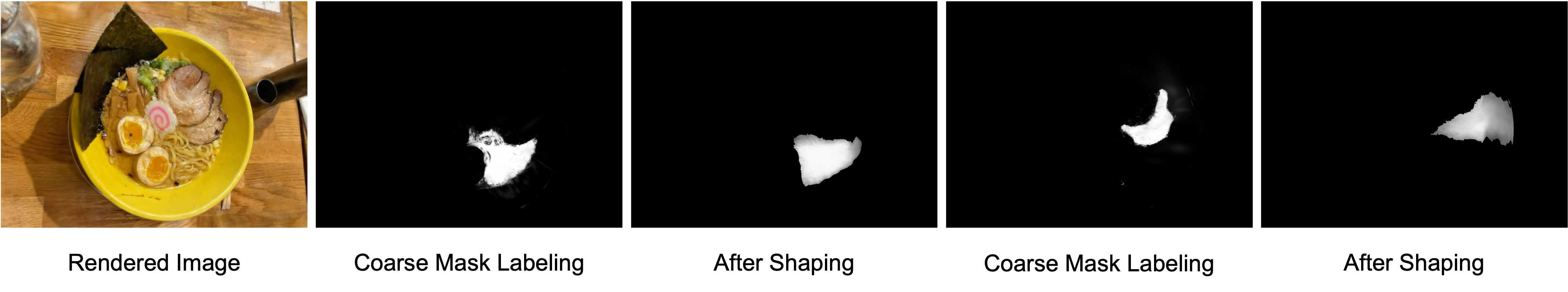
Figure 10: Failure cases in the entangled scenes like ramen [18]. When objects are too close to each other, the mutual information shaping will have negative optimization on segmentation. The segmentation results are worse than the results that we directly use Coarse Mask Labeling.

Fig. 10 shows some failure cases of InfoGaussian. As illustrated, the segmentation results would be exacerbated by the mutual information shaping in InfoGaussian in the ramen scene [18]. The edge of the segmentation becomes round and less sharp, losing the original shape of the objects.

As ramen is a scene where multiple objects are entangled together (e.g., adhering to each other), we speculate that the reason for the deterioration is that we use the centroid $\mathbf{x}$ of Gaussians in the canonical space as the input. The inputs of different objects are very close to each other in this scene, however, we try to make their Jacobians orthogonal during the MI shaping process. Neural networks tend to learn a similar feature for similar results, so it’s hard to optimize the orthogonality perfectly during shaping. In this case, the segmentation results get worse and it also explains why the edge gets blunt. In our future works, we will try to change the way that we look at the motion network. That is, instead of mapping the centroid $x$ in the canonical space to the motion, we would try to adopt a more unique feature for each Gaussian to be the input of the motion network, in order to avoid failure in the entangled scene.

References

- [1] Chong Bao, Yinda Zhang, Bangbang Yang, Tianxing Fan, Zesong Yang, Hujun Bao, Guofeng Zhang, and Zhaopeng Cui. Sine: Semantic-driven image-based nerf editing with prior-guided editing field. 2023 IEEE/CVF Conference on Computer Vision and Pattern Recognition (CVPR), pages 20919–20929, 2023.
- [2] Jonathan T Barron, Ben Mildenhall, Matthew Tancik, Peter Hedman, Ricardo Martin-Brualla, and Pratul P Srinivasan. Mip-nerf: A multiscale representation for anti-aliasing neural radiance fields. In Proceedings of the IEEE/CVF International Conference on Computer Vision, pages 5855–5864, 2021.
- [3] Jonathan T Barron, Ben Mildenhall, Dor Verbin, Pratul P Srinivasan, and Peter Hedman. Mip-nerf 360: Unbounded anti-aliased neural radiance fields. In Proceedings of the IEEE/CVF Conference on Computer Vision and Pattern Recognition, pages 5470–5479, 2022.
- [4] Richard Bronson. Matrix methods: An introduction. 1969.
- [5] Ang Cao and Justin Johnson. Hexplane: A fast representation for dynamic scenes. In Proceedings of the IEEE/CVF Conference on Computer Vision and Pattern Recognition, pages 130–141, 2023.
- [6] Jiazhong Cen, Jiemin Fang, Chen Yang, Lingxi Xie, Xiaopeng Zhang, Wei Shen, and Qi Tian. Segment any 3d gaussians. arXiv preprint arXiv:2312.00860, 2023.
- [7] Yiwen Chen, Zilong Chen, Chi Zhang, Feng Wang, Xiaofeng Yang, Yikai Wang, Zhongang Cai, Lei Yang, Huaping Liu, and Guosheng Lin. Gaussianeditor: Swift and controllable 3d editing with gaussian splatting. ArXiv, abs/2311.14521, 2023.
- [8] Zilong Chen, Feng Wang, and Huaping Liu. Text-to-3d using gaussian splatting. ArXiv, abs/2309.16585, 2023.
- [9] Ho Kei Cheng, Seoung Wug Oh, Brian Price, Alexander Schwing, and Joon-Young Lee. Tracking anything with decoupled video segmentation. In ICCV, 2023.
- [10] Kangle Deng, Andrew Liu, Jun-Yan Zhu, and Deva Ramanan. Depth-supervised nerf: Fewer views and faster training for free. In Proceedings of the IEEE/CVF Conference on Computer Vision and Pattern Recognition, pages 12882–12891, 2022.
- [11] Yuanxing Duan, Fangyin Wei, Qiyu Dai, Yuhang He, Wenzheng Chen, and Baoquan Chen. 4d gaussian splatting: Towards efficient novel view synthesis for dynamic scenes. arXiv preprint arXiv:2402.03307, 2024.
- [12] Sara Fridovich-Keil, Alex Yu, Matthew Tancik, Qinhong Chen, Benjamin Recht, and Angjoo Kanazawa. Plenoxels: Radiance fields without neural networks. In Proceedings of the IEEE/CVF Conference on Computer Vision and Pattern Recognition, pages 5501–5510, 2022.
- [13] Xiao Fu, Shangzhan Zhang, Tianrun Chen, Yichong Lu, Lanyun Zhu, Xiaowei Zhou, Andreas Geiger, and Yiyi Liao. Panoptic nerf: 3d-to-2d label transfer for panoptic urban scene segmentation. In 2022 International Conference on 3D Vision (3DV), pages 1–11. IEEE, 2022.
- [14] Xuan Gao, Chenglai Zhong, Jun Xiang, Yang Hong, Yudong Guo, and Juyong Zhang. Reconstructing personalized semantic facial nerf models from monocular video. ACM Transactions on Graphics (TOG), 41:1 – 12, 2022.
- [15] Stephan J Garbin, Marek Kowalski, Matthew Johnson, Jamie Shotton, and Julien Valentin. Fastnerf: High-fidelity neural rendering at 200fps. In Proceedings of the IEEE/CVF International Conference on Computer Vision, pages 14346–14355, 2021.
- [16] Tero Karras, Miika Aittala, Samuli Laine, Erik Härkönen, Janne Hellsten, Jaakko Lehtinen, and Timo Aila. Alias-free generative adversarial networks. Advances in neural information processing systems, 34:852–863, 2021.
- [17] Bernhard Kerbl, Georgios Kopanas, Thomas Leimkühler, and George Drettakis. 3d gaussian splatting for real-time radiance field rendering. ACM Transactions on Graphics, 42(4), 2023.
- [18] Justin Kerr, Chung Min Kim, Ken Goldberg, Angjoo Kanazawa, and Matthew Tancik. Lerf: Language embedded radiance fields. In International Conference on Computer Vision (ICCV), 2023.
- [19] Diederik P Kingma and Jimmy Ba. Adam: A method for stochastic optimization. arXiv preprint arXiv:1412.6980, 2014.
- [20] Alexander Kirillov, Eric Mintun, Nikhila Ravi, Hanzi Mao, Chloe Rolland, Laura Gustafson, Tete Xiao, Spencer Whitehead, Alexander C. Berg, Wan-Yen Lo, Piotr Dollár, and Ross Girshick. Segment anything. arXiv:2304.02643, 2023.
- [21] Mingrui Li, Shuhong Liu, and Heng Zhou. Sgs-slam: Semantic gaussian splatting for neural dense slam. ArXiv, abs/2402.03246, 2024.
- [22] Xuan Li, Yi-Ling Qiao, Peter Yichen Chen, Krishna Murthy Jatavallabhula, Ming Lin, Chenfanfu Jiang, and Chuang Gan. Pac-nerf: Physics augmented continuum neural radiance fields for geometry-agnostic system identification. ArXiv, abs/2303.05512, 2023.
- [23] Lingjie Liu, Jiatao Gu, Kyaw Zaw Lin, Tat-Seng Chua, and Christian Theobalt. Neural sparse voxel fields. Advances in Neural Information Processing Systems, 33:15651–15663, 2020.
- [24] Ricardo Martin-Brualla, Noha Radwan, Mehdi SM Sajjadi, Jonathan T Barron, Alexey Dosovitskiy, and Daniel Duckworth. Nerf in the wild: Neural radiance fields for unconstrained photo collections. In Proceedings of the IEEE/CVF Conference on Computer Vision and Pattern Recognition, pages 7210–7219, 2021.
- [25] Ben Mildenhall, Pratul P Srinivasan, Matthew Tancik, Jonathan T Barron, Ravi Ramamoorthi, and Ren Ng. Nerf: Representing scenes as neural radiance fields for view synthesis. Communications of the ACM, 65(1):99–106, 2021.
- [26] Thomas Müller, Alex Evans, Christoph Schied, and Alexander Keller. Instant neural graphics primitives with a multiresolution hash encoding. ACM Transactions on Graphics (ToG), 41(4):1–15, 2022.
- [27] Sebastian Nowozin, Botond Cseke, and Ryota Tomioka. f-gan: Training generative neural samplers using variational divergence minimization. Advances in neural information processing systems, 29, 2016.
- [28] Keunhong Park, Utkarsh Sinha, Jonathan T Barron, Sofien Bouaziz, Dan B Goldman, Steven M Seitz, and Ricardo Martin-Brualla. Nerfies: Deformable neural radiance fields. In Proceedings of the IEEE/CVF International Conference on Computer Vision, pages 5865–5874, 2021.
- [29] Keunhong Park, Utkarsh Sinha, Peter Hedman, Jonathan T Barron, Sofien Bouaziz, Dan B Goldman, Ricardo Martin-Brualla, and Steven M Seitz. Hypernerf: A higher-dimensional representation for topologically varying neural radiance fields. arXiv preprint arXiv:2106.13228, 2021.
- [30] Yicong Peng, Yichao Yan, Shengqi Liu, Y. Cheng, Shanyan Guan, Bowen Pan, Guangtao Zhai, and Xiaokang Yang. Cagenerf: Cage-based neural radiance field for generalized 3d deformation and animation. In Neural Information Processing Systems, 2022.
- [31] Albert Pumarola, Enric Corona, Gerard Pons-Moll, and Francesc Moreno-Noguer. D-nerf: Neural radiance fields for dynamic scenes. In Proceedings of the IEEE/CVF Conference on Computer Vision and Pattern Recognition, pages 10318–10327, 2021.
- [32] Yi-Ling Qiao, Alexander Gao, Yi Xu, Yue Feng, Jia-Bin Huang, and Ming C. Lin. Dynamic mesh-aware radiance fields. 2023 IEEE/CVF International Conference on Computer Vision (ICCV), pages 385–396, 2023.
- [33] Christian Reiser, Songyou Peng, Yiyi Liao, and Andreas Geiger. Kilonerf: Speeding up neural radiance fields with thousands of tiny mlps. 2021 IEEE/CVF International Conference on Computer Vision (ICCV), pages 14315–14325, 2021.
- [34] Katja Schwarz, Yiyi Liao, Michael Niemeyer, and Andreas Geiger. Graf: Generative radiance fields for 3d-aware image synthesis. Advances in Neural Information Processing Systems, 33:20154–20166, 2020.
- [35] Jiaxiang Tang, Jiawei Ren, Hang Zhou, Ziwei Liu, and Gang Zeng. Dreamgaussian: Generative gaussian splatting for efficient 3d content creation. arXiv preprint arXiv:2309.16653, 2023.
- [36] Binglun Wang, Niladri Shekhar Dutt, and Niloy Jyoti Mitra. Proteusnerf: Fast lightweight nerf editing using 3d-aware image context. ArXiv, abs/2310.09965, 2023.
- [37] Can Wang, Menglei Chai, Mingming He, Dongdong Chen, and Jing Liao. Clip-nerf: Text-and-image driven manipulation of neural radiance fields. In Proceedings of the IEEE/CVF Conference on Computer Vision and Pattern Recognition, pages 3835–3844, 2022.
- [38] Ruibo Wang, Song Zhang, Ping Huang, Donghai Zhang, and Wei Yan. Semantic is enough: Only semantic information for nerf reconstruction. 2023 IEEE International Conference on Unmanned Systems (ICUS), pages 906–912, 2023.
- [39] Guanjun Wu, Taoran Yi, Jiemin Fang, Lingxi Xie, Xiaopeng Zhang, Wei Wei, Wenyu Liu, Qi Tian, and Xinggang Wang. 4d gaussian splatting for real-time dynamic scene rendering. arXiv preprint arXiv:2310.08528, 2023.
- [40] Tianyi Xie, Zeshun Zong, Yuxin Qiu, Xuan Li, Yutao Feng, Yin Yang, and Chenfanfu Jiang. Physgaussian: Physics-integrated 3d gaussians for generative dynamics. arXiv preprint arXiv:2311.12198, 2023.
- [41] Qiangeng Xu, Zexiang Xu, Julien Philip, Sai Bi, Zhixin Shu, Kalyan Sunkavalli, and Ulrich Neumann. Point-nerf: Point-based neural radiance fields. In Proceedings of the IEEE/CVF Conference on Computer Vision and Pattern Recognition, pages 5438–5448, 2022.
- [42] Xiaomeng Xu, Yanchao Yang, Kaichun Mo, Boxiao Pan, Li Yi, and Leonidas Guibas. Jacobinerf: Nerf shaping with mutual information gradients. In Proceedings of the IEEE/CVF Conference on Computer Vision and Pattern Recognition (CVPR), pages 16498–16507, June 2023.
- [43] Zeyu Yang, Hongye Yang, Zijie Pan, Xiatian Zhu, and Li Zhang. Real-time photorealistic dynamic scene representation and rendering with 4d gaussian splatting. ArXiv, abs/2310.10642, 2023.
- [44] Ziyi Yang, Xinyu Gao, Wen Zhou, Shaohui Jiao, Yuqing Zhang, and Xiaogang Jin. Deformable 3d gaussians for high-fidelity monocular dynamic scene reconstruction. arXiv preprint arXiv:2309.13101, 2023.
- [45] Mingqiao Ye, Martin Danelljan, Fisher Yu, and Lei Ke. Gaussian grouping: Segment and edit anything in 3d scenes. arXiv preprint arXiv:2312.00732, 2023.
- [46] Hsiao yu Chen, Edgar Tretschk, Tuur Stuyck, Petr Kadlecek, Ladislav Kavan, Etienne Vouga, and Christoph Lassner. Virtual elastic objects. 2022 IEEE/CVF Conference on Computer Vision and Pattern Recognition (CVPR), pages 15806–15816, 2022.
- [47] Yu-Jie Yuan, Yang-Tian Sun, Yu-Kun Lai, Yuewen Ma, Rongfei Jia, and Lin Gao. Nerf-editing: Geometry editing of neural radiance fields. 2022 IEEE/CVF Conference on Computer Vision and Pattern Recognition (CVPR), pages 18332–18343, 2022.
- [48] Richard Zhang, Phillip Isola, Alexei A Efros, Eli Shechtman, and Oliver Wang. The unreasonable effectiveness of deep features as a perceptual metric. In Proceedings of the IEEE conference on computer vision and pattern recognition, pages 586–595, 2018.
- [49] Xiaoshuai Zhang, Abhijit Kundu, Thomas Funkhouser, Leonidas Guibas, Hao Su, and Kyle Genova. Nerflets: Local radiance fields for efficient structure-aware 3d scene representation from 2d supervision. In Proceedings of the IEEE/CVF Conference on Computer Vision and Pattern Recognition, pages 8274–8284, 2023.
- [50] Shuaifeng Zhi, Tristan Laidlow, Stefan Leutenegger, and Andrew J Davison. In-place scene labelling and understanding with implicit scene representation. In Proceedings of the IEEE/CVF International Conference on Computer Vision, pages 15838–15847, 2021.
- [51] Shijie Zhou, Haoran Chang, Sicheng Jiang, Zhiwen Fan, Zehao Zhu, Dejia Xu, Pradyumna Chari, Suya You, Zhangyang Wang, and Achuta Kadambi. Feature 3dgs: Supercharging 3d gaussian splatting to enable distilled feature fields. arXiv preprint arXiv:2312.03203, 2023.