Information Theoretic Guarantees For Policy Alignment
In Large Language Models
Abstract.
Policy alignment of large language models refers to constrained policy optimization, where the policy is optimized to maximize a reward while staying close to a reference policy with respect to an -divergence such as the divergence. The best of alignment policy selects a sample from the reference policy that has the maximum reward among independent samples. For both cases (policy alignment and best of ), recent works showed empirically that the reward improvement of the aligned policy on the reference one scales like , with an explicit bound in on the for the best of policy. We show in this paper that the information theoretic upper bound holds if the reward under the reference policy has sub-gaussian tails. Moreover, we prove for the best of policy, that the upper bound can be obtained for any -divergence via a reduction to exponential order statistics owing to the Rényi representation of order statistics, and a data processing inequality. If additional information is known on the tails of the aligned policy we show that tighter control on the reward improvement can be obtained via the Rényi divergence. Finally we demonstrate how these upper bounds transfer from proxy rewards to golden rewards which results in a decrease in the golden reward improvement due to overestimation and approximation errors of the proxy reward.
1. Introduction
Aligning Large Language Models (LLMs) with human preferences allows a tradeoff between maintaining the utility of the pre-trained reference model and the alignment of the model with human values such as safety or other socio-technical considerations. Alignment is becoming a crucial step in LLMs training pipeline, especially as these models are leveraged in decision making as well as becoming more and more accessible to the general public. Policy alignment starts by learning a reward model that predicts human preferences, these reward models are typically fine-tuned LLMs that are trained on pairwise human preference data (Christiano et al., 2017; Stiennon et al., 2020; Ouyang et al., 2022; Bai et al., 2022). The reward is then optimized using training time alignment i.e via policy gradient based reinforcement learning leading to the so called Reinforcemnent Learning from Human Feedback (RLHF) (Christiano et al., 2017). RLHF ensures that the reward is maximized while the policy stays close to the initial reference policy in the sense of the Kullback-Leibler divergence . Other variants of these training time alignment have been proposed via direct preference optimization (Rafailov et al., 2024) (Zhao et al., 2023) (Ethayarajh et al., 2024). Another important paradigm for optimizing the reward is test time alignment via best of sampling from the reference policy and retaining the sample that maximizes the reward. The resulting policy is known as the best of policy. The best of policy is also used in controlled decoding settings (Yang and Klein, 2021; Mudgal et al., 2023) and in fine-tuning LLMs to match the best of policy responses (Touvron et al., 2023).
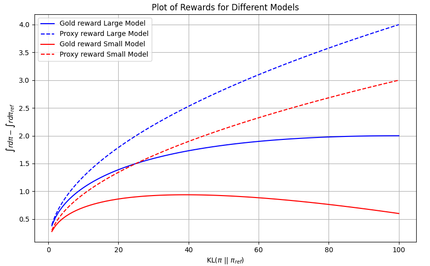
(Gao et al., 2023) and (Hilton and Gao, 2022) studied the scaling laws of reward models optimization in both the RL and the best of setups. (Gao et al., 2023) distinguished between “golden reward” that can be thought of as the golden human preference and “proxy reward” which is trained to predict the golden reward. For proxy rewards (Gao et al., 2023) found experimentally for both RL and best of policies that the reward improvement on the reference policy scales as . Similar observations for reward improvement scaling in RL were made in (Bai et al., 2022). For golden rewards, (Gao et al., 2023) showed for both RL and best of policies that LLMs that optimize the proxy reward suffer from over-optimization in the sense that as the policy drifts from the reference policy, optimizing the proxy reward results in deterioration of the golden reward. This phenomena is referred to in (Gao et al., 2023) (Hilton and Gao, 2022) as Goodhart’s law. A qualitative plot of scaling laws discovered in (Gao et al., 2023) is given in Figure 1. For the best of policy, most works in this space assumed that (Stiennon et al., 2020; Coste et al., 2024; Nakano et al., 2021; Go et al., 2024; Gao et al., 2023). Recently Beirami et al. (2024) showed that this is in fact an inequality under the assumption that the reward is one to one map (a bijection) and for finite alphabets. The main contribution of this papers are :
-
(1)
We provide in Theorem 17 in Section 2 a new proof for the best of policy inequality and show via a reduction to exponential random variables that it is a consequence of the data processing inequality of the divergence. We extend this inequality beyond the setup of (Beirami et al., 2024) of one to one rewards and finite alphabets to a more realistic setup of surjective rewards and beyond finite alphabets. We also give conditions under which the equality is met, and extend those inequalities to -divergences and Rényi divergences.
-
(2)
We show in Section 3 that the scaling laws on policy improvement versus of (Gao et al., 2023) are information theoretic upper bounds and are consequences of transportation inequalities with the divergence under sub-gaussian tails of the reward under the reference policy. We discuss how the dependency on is driven only by the tails of the reward under the reference model, and cannot be improved by a better alignment algorithm and can only be improved if the tails of the reference rewards are fatter than sub-gaussian such as sub-gamma or sub-exponential tails.
- (3)
- (4)
2. The Alignment Problem
2.1. RLHF: A Constrained Policy Optimization Problem
Let be the space of prompts and be the space of responses from a LLM conditioned on a prompt . The reference LLM is represented as policy , i.e as a conditional probability on given a prompt . Let be a distribution on prompts, and a a reward, , represents a safety or alignment objective that is desirable to maximize.
Given a reference policy , the goal of alignment is to find a policy that maximizes the reward and that it is still close to the original reference policy for some positive :
| (1) |
where With some abuse of notation, we write and . Let be joint probability defined on that has as marginal on . Hence we can write the alignment problem (1) in a more compact way as follows:
| (2) |
For , we can also write a penalized form of this constrained policy optimization problem as follows: It is easy to see that the optimal policy of the penalized problem is given by:
| (3) |
The constrained problem (2) has a similar solution (See for e.g (Yang et al., 2024)):
| (4) |
where is a lagrangian that satisfies
2.2. Best of Policy Alignment
Let be the random variable associated with prompts such that Law(. Let be the random variable associated with the conditional response of given . Define the conditional reward of the reference policy :
we assume that admits a CDF denoted as and let be its quantile:
Let be independent samples from . We define the best of reward as follows:
| (5) |
this the maximum of iid random variables with a common CDF . The best of policy corresponds to We note the law of . is referred to as the best of alignment policy. We consider two setups for the reward:
Assumption 1.
We assume that the reward is a one to one map for a fixed , and admits an inverse such that .
This assumption was considered in (Beirami et al., 2024). Nevertheless this assumption is strong and not usually meet in practice, we weaken this assumption to the following:
Assumption 2.
We assume that there is a stochastic map such that and .
Under Assumption 2, the reward can be surjective which is more realistic but we assume that there is a stochastic map that ensures invertibility not point-wise but on a distribution level. Our assumption means that we have conditionnaly on : form a markov chain i.e exists so that and
Best of Policy Guarantees: A reduction to Exponentials. In what follows for random variables with laws we write interchangeably: Let us start by looking at the divergence between the conditional reward of the best of policy and that of the reference policy. Let , the optimal transport map from the exponential distribution to (See for example Theorem 2.5 in (Santambrogio, 2015): is atomless, but can be discrete valued) allows us to write:
| (6) |
where means equality in distribution. On the other hand, let be the order statistics of the rewards of independent samples , . The order statistics refer to sorting the random variable from the minimum (index ) to the maximum (index ). Consider independent exponential , where , and their order statistics . The Rényi representation of order statistics (Rényi, 1953), similar to the Optimal Transport (OT) representation allows us to express the distribution of the order statistics of the rewards in terms of the order statistics of exponentials as follows:
| (7) |
The central idea in the Rényi representation is that the mapping is monotonic and hence ordering preserving and by the OT representation each component is distributed as . See (Boucheron and Thomas, 2012) for more account on the Rényi representation of order statistics.
Hence using the OT representation in (6) and the Rényi representation of the maximum (7), we can reduce the between the rewards to a on functions of exponentials and their order statistics:
| (8) |
where
Under Assumption 1 we can write samples from the best of policy as and from the reference policy as Hence we have by the data processing inequality (DPI) for the divergence (See for e.g (Polyanskiy and Wu, 2023)) under Assumption 1:
| (9) |
Recall that , is one to one. If the space is finite, has a discontinuous CDF hence not strictly monotonic. It follows that its quantile is not a one to one map and as a result is not a one to one map and hence we have by DPI (that is an inequality in this case since is not one to one):
| (10) |
If the space is infinite and we assume that is continuous and strictly monotonic then is a one to one map, and as a result is a one to one map and the DPI is an equality in this case:
| (11) |
Hence under Assumption 1 and for finite combining (9) and (10) we have:
| (12) |
and under Assumption 1 and for infinite and assuming is continuous and strictly monotonic, combining (9) and (11) we have:
| (13) |
Under the more realistic Assumption 2 we can also apply the DPI on the stochastic map , since DPI also holds for stochastic maps ( under our assumption see for example (van Erven and Harremos, 2014) Example 2)
| (14) |
and hence under Assumption 2 regardless whether is a one to one map or not, thus we have: . The following Lemma gives a closed form expression for :
Lemma 1 ( Between Exponential and Maximum of Exponentials).
Let , and be iid exponentials and their maximum, we have:
| (15) |
Hence we conclude with the following result:
Theorem 1.
Proof.
Combining Lemma 15, the analysis above and taking expectation on we obtain the result. ∎
Beirami et al. (2024) showed this result under condition (i) which is not a realistic setting and used the finiteness of to provide a direct proof. Our analysis via chaining DPI and using OT and Rényi representations to reduce the problem to exponentials allows us to extend the result to a more realistic setup under condition (ii) i.e the existence of a stochastic “inverse", without any assumption on . Furthermore we unveil under which conditions the equality holds that was assumed to hold in previous works (Stiennon et al., 2020) (Coste et al., 2024; Nakano et al., 2021; Go et al., 2024) (Hilton and Gao, 2022) (Gao et al., 2023).
Our approach of reduction to exponentials using Rényi representation of order statistics and data processing inequalities extends to bounding the - divergence as well as the Rényi divergence. The Rényi divergence for is defined as follows:
the limit as coincides with , i.e: . These bounds are summarized in Table 1. Full proofs and theorems are in the Appendix.
| Divergence | Bound on | |
| Chi-squared | ||
| Total Variation | ||
| Hellinger distance | ||
| Forward | ||
| Rényi Divergence | NA |
Best of -Policy Dominance on the Reference Policy. The following proposition shows that the best of policy leads to an improved reward on average:
Proposition 1.
dominates in the first order dominance that is dominates on all quantiles:
It follows that we have .
Best of Policy and RL Policy The following proposition discusses the sub-optimality of the best of policy with respect to the alignment RL objective given in (1):
Proposition 2.
Assume a bounded reward in . For and the best of policy and the Constrained RL policy (given in (4)) satisfy:
A similar asymptotic result appeared in (Yang et al., 2024) for , showing as , , we provide here a non asymptotic result for finite and finite .
3. Reward Improvement Guarantees Through Transportation Inequalities
Notations
Let be a real random variable. The logarithmic moment generating function of is defined as follows for :
is said to be sub-Gaussian with variance if :
We denote the set of sub-Gaussian random variables with variance .
is said to be sub-Gamma on the right tail with variance factor and a scale parameter if :
We denote the set of left and right tailed sub-Gamma random variables. Sub-gamma tails can be thought as an interpolation between sub-Gaussian and sub-exponential tails.
Scaling Laws in Alignment
It has been observed empirically (Coste et al., 2024; Nakano et al., 2021; Go et al., 2024; Hilton and Gao, 2022; Gao et al., 2023) that optimal RL policy satisfy the following inequality for a constant :
A similar scaling for best of policy :
and those bounds are oftentimes tight even when empirically estimated from samples. This hints that those bounds are information theoretic and independent of the alignment problem. Indeed if the reward was bounded, a simple application of Pinsker inequality gives rise to scaling. Let be the total variation distance, we have: Hence we can deduce that for bounded rewards with norm infinity that:
Nevertheless this boundedness assumption on the reward is not realistic, since most reward models are unbounded: quoting Lambert et al. (2024) “ implemented by appending a linear layer to predict one logit or removing the final decoding layers and replacing them with a linear layer” and hence the reward is unbounded by construction. We will show in what follows that those scalings laws are tied to the tails of the reward under the reference policy and are instances of transportation inequalities.
3.1. Transportation Inequalities with Divergence
For a policy and for a reward function , we note , the push-forward map of through . The reader is referred to Appendix D.1 for background on transportation inequalities and how they are derived from the so-called Donsker-Varadhan variational representation of the divergence. The following Proposition is an application of Lemma 4.14 in (Boucheron et al., 2013)):
Proposition 3 (Transportation Inequalities).
The following inequalities hold depending on the tails of :
-
(1)
Assume that . For any that is absolutely continuous with respect to , and such that then we have:
-
(2)
Assume that . For any that is absolutely continuous with respect to , and such that then we have:
In particular we have the following Corollary:
Corollary 1 (Expected Reward Improvement).
If the following holds for the optimal RL policy and for the best of policy :
-
(1)
For the optimal RL policy we have:
-
(2)
For the Best of policy , under Assumption 2 we have:
A similar statement holds under sub-gamma tails of the reward of the reference model. We turn now to providing a bound in high probability on the empirical reward improvement of RL:
Remark 1.
Item (1) in Corollary 1 shows that the provides an upper bound on the reward improvement of the alignment under subgaussian tails of the reference reward. Under subgaussian tails of the reference, this information theoretic barrier can not be broken with a better algorithm. On way to improve on the ceiling is by aiming at having a reference model with a reward that has subgamma tails to improve the upper limit to , or to subexponential tails to be linear in the . Item (2) can be seen as a refinement on the classical upper bound on the expectation of maximum of subgaussians see for e.g Corollary 2.6 in (Boucheron et al., 2013). If in addition is positive and for we have for , , where (where is a variance) , then we have a matching lower bound for that scales with for sufficiently large (See (Kamath, 2015)).
The following Theorem gives high probability bounds for the excess reward when estimated from empirical samples:
Theorem 2 (High Probability Empirical Reward Improvement For RL).
Assume . Let and . Let be the optimal policy of the penalized RL problem given in Equation (3). Let and be the rewards evaluated at samples from and . Assume that the -Rényi divergence and are both finite. The following inequality holds with probability at least :
Note that in Theorem 2, we did not make any assumptions on the tails of and we see that this results in a biased concentration inequality with a non-negative bias . For the best of policy, if the reward was positive and has a folded normal distribution (absolute value of gaussians), (Boucheron and Thomas, 2012) provides concentration bounds, owing to the subgamma tails of the maximum of absolute value of Gaussians.
3.2. Tail Adaptive Transportation Inequalities with the Rényi Divergence
An important question on the tightness of the bounds rises from the bounds in Corollary 1. We answer this question by considering additional information on the tails of the reward under the policy , and we obtain tail adaptive bounds that are eventually tighter than the one in Corollary 1. Our new bounds leverage a variational representation of the Rényi divergence that uses the logarithmic moment generating function of both measures at hand.
Preliminaries for the Rényi Divergence
The Donsker-Varadahn representation of was crucial in deriving transportation inequalities. In Shayevitz (2011) the following variational form is given for the Rényi divergence in terms of the divergence, for all
| (18) |
A similar variational form was rediscovered in (Anantharam, 2018). Finally a Donsker-Varadahn-Rényi representation of was given in (Birrell et al., 2021). For all we have :
| (19) |
where Birrell et al. (2021) presents a direct proof of this formulation without exploring its link to the representation given in (18), we show in what follows an elementary proof via convex conjugacy, the duality relationship between equations (18) and (19).
We collect in what follows elementary lemmas that will be instrumental to derive transportation inequalities in terms of the Rényi divergence. Proofs are given in the Appendix.
Lemma 2.
Let , and define . We have for all and for
Lemma 3.
The following limit holds for the Rényi divergence
Transportation Inequalities with Rényi Divergence.
The following theorem shows that when considering the tails of we can obtain tighter upper bounds using the Rényi divergence that is more tail adaptive:
Theorem 4 (Tail Adaptive Transportation Inequalities).
Let . Assume and then we have for all :
| (20) |
In particular if there exits such that , then the tail adaptive upper bound given in Equation (20) is tighter than the one provided by the tails of only i.e . Note that this is possible because is increasing in (van Erven and Harremos, 2014), i.e , and . Note that taking limits (applying Lemma 3) and , and taking the minimum of the upper bounds we obtain:
this inequality can be also obtained by applying Proposition 3 twice: on the tails of and respectively.
Another important implication of Theorem 4, other than tighter than upper bound, is that if we were to change the RL alignment problem (1) to be constrained by instead of , we may end up with a smaller upper limit on the reward improvement. This constrained alignment may lead to a policy that under-performs when compared to a policy obtained with the constraint. This was indeed observed experimentally in (Wang et al., 2024) that used constraints with - divergences for (that are related to Rényi divergences) and noticed a degradation in the reward improvement w.r.t the policy obtained using constraints.
4. Transportation Inequality Transfer From Proxy to Golden Reward
As we saw in the previous sections, the tightness of upper bound in alignment can be due to the tails of the reward of the aligned policy (Theorem 4) and to the concentration around the mean in finite sample size (Theorem 2). Another important consideration is the mismatch between the golden reward that one desires to maximize that is expensive and difficult to obtain (for example human evaluation) and a proxy reward that approximates . The proxy reward is used instead of in RL and in best of policy. While we may know the tails of the reward of the reference and aligned model, we don’t have access to this information on the golden reward . We show in this section how to transfer transportation inequalities from to for RL and Best of policy.
Proposition 4 ( Transportation Inequality for RL Policy ).
The following inequality holds:
Assume , and there exists such that:
then we have:
Note that is interpreted here as an interpolation between the mean and the maximum of its argument on the support of (Proposition 9 in (Feydy et al., 2018)). Indeed as , this boils down to the mean on and this boils down to . Our assumption means that overestimates and the overestimation is accentuated as we drift from on which was learned. This assumption echoes findings in (Gao et al., 2023) that show that the transportation inequalities suffer from overestimation of proxy reward models of the golden reward (See Figure 8 in (Gao et al., 2023)).
Note that in Proposition 4, we are evaluating the golden reward improvement when using the proxy reward optimal policy . We see that the golden reward of the RL policy inherits the transportation inequality from the proxy one but the improvement of the reward is hindered by possible overestimation of the golden reward by the proxy model. This explains the dip in performance as measured by the golden reward depicted in Figure 1 and reported in (Gao et al., 2023).
Proposition 5 ( Transportation Inequality for Best of Policy).
Let . Let be a surrogate reward such that and assume then the best of policy satisfies:
Transportation inequalities transfers for the best of policy from to and pays only an additional error term , an upper bound of this total variation as a function of is given in Table 1. As mentioned in remark 1, if we have lower bounds on the tail of the reference reward, then we also have a lower bound on the reward improvement that scales like This is in line with empirical findings in (Hilton and Gao, 2022) (Gao et al., 2023) that showed that best of policy is resilient as the reward model gets closer to .
5. Conclusion
We presented in this paper a comprehensive information theoretical analysis of policy alignment using reward optimization with RL and best of sampling. We showed for best of a bound on under realistic assumptions on the reward. Our analysis showed that the alignment reward improvement, is intrinsically constrained by the tails of the reward under the reference policy and controlling the divergence results in an upper bound of the policy improvement. We showed that the bound may not be tight if the tails of the optimized policy satisfy a condition expressed via Rényi divergence. We also explained the deterioration of the golden reward via overestimation of the proxy reward.
References
- Anantharam [2018] V. Anantharam. A variational characterization of rényi divergences. IEEE Transactions on Information Theory, 64(11):6979–6989, 2018.
- Bai et al. [2022] Y. Bai, A. Jones, K. Ndousse, A. Askell, A. Chen, N. DasSarma, D. Drain, S. Fort, D. Ganguli, T. Henighan, et al. Training a helpful and harmless assistant with reinforcement learning from human feedback. arXiv preprint arXiv:2204.05862, 2022.
- Beirami et al. [2024] A. Beirami, A. Agarwal, J. Berant, A. D’Amour, J. Eisenstein, C. Nagpal, and A. T. Suresh. Theoretical guarantees on the best-of-n alignment policy, 2024.
- Birrell et al. [2021] J. Birrell, P. Dupuis, M. A. Katsoulakis, L. Rey-Bellet, and J. Wang. Variational representations and neural network estimation of rényi divergences. SIAM Journal on Mathematics of Data Science, 3(4):1093–1116, 2021.
- Boucheron and Thomas [2012] S. Boucheron and M. Thomas. Concentration inequalities for order statistics. 2012.
- Boucheron et al. [2013] S. Boucheron, G. Lugosi, and P. Massart. Concentration Inequalities - A Nonasymptotic Theory of Independence. Oxford University Press, 2013. ISBN 978-0-19-953525-5. doi: 10.1093/ACPROF:OSO/9780199535255.001.0001. URL https://doi.org/10.1093/acprof:oso/9780199535255.001.0001.
- Christiano et al. [2017] P. F. Christiano, J. Leike, T. Brown, M. Martic, S. Legg, and D. Amodei. Deep reinforcement learning from human preferences. In I. Guyon, U. V. Luxburg, S. Bengio, H. Wallach, R. Fergus, S. Vishwanathan, and R. Garnett, editors, Advances in Neural Information Processing Systems, volume 30. Curran Associates, Inc., 2017. URL https://proceedings.neurips.cc/paper_files/paper/2017/file/d5e2c0adad503c91f91df240d0cd4e49-Paper.pdf.
- Coste et al. [2024] T. Coste, U. Anwar, R. Kirk, and D. Krueger. Reward model ensembles help mitigate overoptimization. In The Twelfth International Conference on Learning Representations, 2024. URL https://openreview.net/forum?id=dcjtMYkpXx.
- Ethayarajh et al. [2024] K. Ethayarajh, W. Xu, N. Muennighoff, D. Jurafsky, and D. Kiela. Kto: Model alignment as prospect theoretic optimization. arXiv preprint arXiv:2402.01306, 2024.
- Feydy et al. [2018] J. Feydy, T. Séjourné, F.-X. Vialard, S. ichi Amari, A. Trouvé, and G. Peyré. Interpolating between optimal transport and mmd using sinkhorn divergences, 2018.
- Gao et al. [2023] L. Gao, J. Schulman, and J. Hilton. Scaling laws for reward model overoptimization. In International Conference on Machine Learning, pages 10835–10866. PMLR, 2023.
- Go et al. [2024] D. Go, T. Korbak, G. Kruszewski, J. Rozen, and M. Dymetman. Compositional preference models for aligning LMs. In The Twelfth International Conference on Learning Representations, 2024. URL https://openreview.net/forum?id=tiiAzqi6Ol.
- Hilton and Gao [2022] J. Hilton and L. Gao. Measuring goodhart’s law, 2022.
- Kamath [2015] G. Kamath. Bounds on the expectation of the maximum of samples from a gaussian. URL http://www. gautamkamath. com/writings/gaussian max. pdf, 10:20–30, 2015.
- Lambert et al. [2024] N. Lambert, V. Pyatkin, J. Morrison, L. Miranda, B. Y. Lin, K. Chandu, N. Dziri, S. Kumar, T. Zick, Y. Choi, N. A. Smith, and H. Hajishirzi. Rewardbench: Evaluating reward models for language modeling, 2024.
- Mudgal et al. [2023] S. Mudgal, J. Lee, H. Ganapathy, Y. Li, T. Wang, Y. Huang, Z. Chen, H.-T. Cheng, M. Collins, T. Strohman, et al. Controlled decoding from language models. arXiv preprint arXiv:2310.17022, 2023.
- Nakano et al. [2021] R. Nakano, J. Hilton, S. Balaji, J. Wu, L. Ouyang, C. Kim, C. Hesse, S. Jain, V. Kosaraju, W. Saunders, et al. Webgpt: Browser-assisted question-answering with human feedback. arXiv preprint arXiv:2112.09332, 2021.
- Ouyang et al. [2022] L. Ouyang, J. Wu, X. Jiang, D. Almeida, C. Wainwright, P. Mishkin, C. Zhang, S. Agarwal, K. Slama, A. Ray, et al. Training language models to follow instructions with human feedback. Advances in Neural Information Processing Systems, 35:27730–27744, 2022.
- Polyanskiy and Wu [2023] Y. Polyanskiy and Y. Wu. Information theory: From coding to learning, 2023.
- Rafailov et al. [2024] R. Rafailov, A. Sharma, E. Mitchell, C. D. Manning, S. Ermon, and C. Finn. Direct preference optimization: Your language model is secretly a reward model. Advances in Neural Information Processing Systems, 36, 2024.
- Rényi [1953] A. Rényi. On the theory of order statistics. Acta Mathematica Academiae Scientiarum Hungarica, 4:191–231, 1953. URL https://api.semanticscholar.org/CorpusID:123132570.
- Santambrogio [2015] F. Santambrogio. Optimal Transport for Applied Mathematicians: Calculus of Variations, PDEs, and Modeling. Birkhäuser, Cham, 2015. ISBN 9783319208275. doi: 10.1007/978-3-319-20828-2.
- Shayevitz [2011] O. Shayevitz. On rényi measures and hypothesis testing. In 2011 IEEE International Symposium on Information Theory Proceedings, pages 894–898, 2011. doi: 10.1109/ISIT.2011.6034266.
- Stiennon et al. [2020] N. Stiennon, L. Ouyang, J. Wu, D. Ziegler, R. Lowe, C. Voss, A. Radford, D. Amodei, and P. F. Christiano. Learning to summarize with human feedback. Advances in Neural Information Processing Systems, 33:3008–3021, 2020.
- Touvron et al. [2023] H. Touvron, L. Martin, K. Stone, P. Albert, A. Almahairi, Y. Babaei, N. Bashlykov, S. Batra, P. Bhargava, S. Bhosale, et al. Llama 2: Open foundation and fine-tuned chat models. arXiv preprint arXiv:2307.09288, 2023.
- van Erven and Harremos [2014] T. van Erven and P. Harremos. Rényi divergence and kullback-leibler divergence. IEEE Transactions on Information Theory, 60(7):3797–3820, 2014. doi: 10.1109/TIT.2014.2320500.
- Wang et al. [2024] C. Wang, Y. Jiang, C. Yang, H. Liu, and Y. Chen. Beyond reverse KL: Generalizing direct preference optimization with diverse divergence constraints. In The Twelfth International Conference on Learning Representations, 2024. URL https://openreview.net/forum?id=2cRzmWXK9N.
- Yang et al. [2024] J. Q. Yang, S. Salamatian, Z. Sun, A. T. Suresh, and A. Beirami. Asymptotics of language model alignment, 2024.
- Yang and Klein [2021] K. Yang and D. Klein. FUDGE: Controlled text generation with future discriminators. In K. Toutanova, A. Rumshisky, L. Zettlemoyer, D. Hakkani-Tur, I. Beltagy, S. Bethard, R. Cotterell, T. Chakraborty, and Y. Zhou, editors, Proceedings of the 2021 Conference of the North American Chapter of the Association for Computational Linguistics: Human Language Technologies, pages 3511–3535, Online, June 2021. Association for Computational Linguistics. doi: 10.18653/v1/2021.naacl-main.276. URL https://aclanthology.org/2021.naacl-main.276.
- Zhao et al. [2023] Y. Zhao, M. Khalman, R. Joshi, S. Narayan, M. Saleh, and P. J. Liu. Calibrating sequence likelihood improves conditional language generation. In The Eleventh International Conference on Learning Representations, 2023. URL https://openreview.net/forum?id=0qSOodKmJaN.
Appendix A Broader Impact and Limitations
We believe this work explaining scaling laws for reward models and alignment will give practitioners insights regarding the limits of what is attainable via alignment. All assumptions under which our statements hold are given. We don’t see any negative societal impact of our work.
Appendix B Proofs For Best of Policy
B.1. Best of Policy Guarantees
Proof of Lemma 15.
We have . Note that the CDF of maximum of exponential and hence . Hence we have:
Let , we have . It follows that :
∎
B.2. Best of n Policy f divergence and Rényi Divergence
Best of Policy divergence and Renyi divergence Guarantees
Given that our proof technique relies on DPI and Rényi representation, we show that similar results hold for any -divergence and for the Rényi divergence:
| (21) |
where is convex and . Hence we have by DPI for -divergences:
Proof of Theorem 5.
| (23) | ||||
| (24) | ||||
| (25) | ||||
| (26) | ||||
| (27) |
In particular we have the following bounds for common divergences:
-
•
For we obtain the KL divergence and we have the result:
-
•
For we obtain the chi-squared divergence and we have: .
-
•
For , we obtain the total variation distance and we have: where , i.e . Hence the TV is .
-
•
For we have the hellinger distance:
-
•
For , we obtain the forward KL and we have : .
∎
Guarantees with Rényi Divergence
Turning now to the Rényi divergence for :
the limit as .
Proof of Theorem 28.
Applying DPI that holds also for the Rényi divergence twice from to and from to we obtain :
Let we have
∎
From Renyi to KL guarantees
Let , and , we have , we have , hence applying L’Hôpital rule we have: . Hence we recover the result for the divergence.
B.3. Best of Dominance
Proof of Proposition 1 .
, which means also that , which means that dominates in the first stochastic order : , which means there exists a coupling between and , , such that , for all . On the other hand By Rényi and Monge map representations we have: and , given that is non decreasing the same coupling guarantees that , for all and Hence .
∎
Corollary 2.
Best of n-polciy has higher expectation :
and is a safer policy, let the Tail Value at Risk be:
We have
Proof of Corollary 2.
First order dominance implies second order dominance (i.e by integrating quantiles). Expectation is obtained for . ∎
Appendix C Best of and RL Policy
Proof of Proposition 2.
We fix here
On the other hand by optimality of we have:
and hence we have:
We choose such that :
and we conclude choosing therefore for that choice of that:
On the other hand we have:
where we used the following fact, followed by Jensen inequality :
Assume that the reward is bounded hence we have by Hoeffding inequality :
Hence we have:
∎
Appendix D Transportation Inequalities and KL Divergence
D.1. Transportation Inequalities with KL
The following Lemma (Lemma 4.14 in [Boucheron et al., 2013]) uses the Donsker-Varadhan representation of the KL divergence to obtain bounds on the change of measure , and using the tails of .
Lemma 4 (Lemma 4.14 in [Boucheron et al., 2013]).
Let be a convex and continuously differentiable function on a possibly unbounded interval , and assume . Define for every , the convex conjugate , and let . Then the following statements are equivalent:
(i) For
(ii) For any probability measure that is absolutely continuous with respect to and such that :
Lemma 5 ( Inverse of the conjugate [Boucheron et al., 2013]).
-
(1)
If , we have for
-
(2)
If , we have for .
We give here a direct proof for the subgaussian case:
Proof.
By the Donsker Varadhan representation of the we have:
Fix and and define for
We omit in what follows and , but the reader can assume from here on that and are conditioned on . Note that and we assume subgaussian. Note that
where the moment generating function of the reward under the reference policy. is subgaussian we have for all :
Hence and we have for all and for all and :
or equivalently:
Finally we have for for all :
| (29) |
Being a subgaussian, the MGF of is bounded as follows:
Hence we have for :
Integrating over we obtain for all and all :
Define :
minimizing the upper bound for , taking derivative gives . Taking is the minimizer. Putting this in the bound we have finally for all rewards for all :
| (30) |
∎
Proof of Corollary 1.
(i) This follows from optimality of and applying the transportation inequality for gaussian tail.
(ii) This follows from applying Corollary 2 (best of policy has larger mean ) and 17 for bounding the .
∎
Proof of Theorem 2.
For the penalized RL we have by optimality:
It follows that :
| (31) |
On the other hand by the variational representation of the Rényi divergence we have:
| (32) |
Summing Equations (31) and (32) we obtain a bound on the moment generating function at of (this is not a uniform bound , it holds only for ):
| (33) |
Let us assume we have therefore the following bound on the logarithmic moment generation function at
Let , the reward evaluation of independent samples of we have:
| (34) |
Let , hence we have for :
Now turning to , since we have for every :
Hence we have with probability at least :
∎
Appendix E Proofs for Transportation Inequalities and Rényi Divergence
Proposition 6 (Fenchel Conjugate Propreties).
Let and be convex functions on a space and , be their convex conjugates defined on . We have:
-
(1)
Let we have:
(35) -
(2)
Duality:
(36) -
(3)
Toland Duality:
(37)
Proof of Theorem 3.
Let , let , the Fenchel conjugate of is defined for bounded and measurable function as follows It follows by 1) in Proposition 6 that : .
For :
The objective function in (18) is the sum of convex functions: , by (2) in Proposition 6, we have by duality:
Replacing by does not change the value of the sup and hence we obtain:
dividing by both sides we obtain for :
Proof of Lemma 3.
Note that we have for , (See Proposition 2 in van Erven and Harremos [2014]). Taking limits we obtain ∎
Proof of Theorem 4 .
For , we have for all :
| (38) |
Assuming is bounded then we have and are sub-Gaussian with parameter . Hence we have for :
Fix a finite . For and and , consider , thanks to subgaussianity and boundedness of , for all . Hence we have by Equation (38) for all :
we have by sub-Gaussianity:
It follows that for all
Integrating over we obtain:
Finally we have:
minimizing over : we obtain , is free of choice, choosing , gives that is the minimizer and hence we have for all :
∎
Appendix F Goodhart Laws
Proof of Proposition 4.
We have by duality:
hence for we have:
Hence:
On the other hand by optimality of we have:
Hence we have:
It follows that:
Hence we have finally:
The proof follows from using the subgaussianity of and the assumption on the soft max. ∎
Proof of Proposition 5.
For , we have:
and
By the data processing inequality we have: If has subguassian tails under than we have:
∎