The dynamics of machine-learned “softness” in supercooled liquids describe dynamical heterogeneity
Abstract
The dynamics of supercooled liquids slow down and become increasingly heterogeneous as they are cooled. Recently, local structural variables identified using machine learning, such as “softness,” have emerged as predictors of local dynamics. Here we construct a model using softness to describe the structural origins of dynamical heterogeneity in supercooled liquids. In our model, the probability of particles to rearrange is determined by their softness, and each rearrangement induces changes in the softness of nearby particles, describing facilitation. We show how to ensure that these changes respect the underlying time-reversal symmetry of the liquid’s dynamics. The model reproduces the salient features of dynamical heterogeneity, and demonstrates how long-ranged dynamical correlations can emerge at long time scales from a relatively short softness correlation length.
I Introduction
Sufficiently rapid cooling of a liquid below the melting temperature prevents crystallization and produces a supercooled liquid. While such a state is not in equilibrium since the true equilibrium state is a crystal, it converges to a well-defined metastable “equilibrium” state at sufficiently long times [1], which obeys detailed balance due to the time-reversibility of the microscopic equations of motion. This state exhibits progressively more dramatic dynamical phenomena with decreasing temperature with little accompanying change of structure, namely: (1) The time required to reach “equilibrium,” the relaxation time, grows rapidly with decreasing temperature [2, 3, 4]. In systems known as fragile liquids, this growth is faster than an Arrhenius law. (2) Supercooled liquids are dynamically heterogeneous, with some regions that are relatively mobile (and that tend to relax quickly) and others that are nearly immobile and do not relax. The strength of this heterogeneity grows as is decreased [5, 6, 7, 8]. (3) At sufficiently low temperatures, the system cannot reach “equilibrium” and falls into the glass state, where the properties depend on the time since the system was quenched into the glass (the age of the glass) [9, 10, 11, 12, 13, 14].
The super-Arrhenius growth of relaxation time in fragile glassformers suggests that a characteristic energy barrier grows as is lowered [15]. Such an energy barrier should be structural in origin. Moreover, isoconfigurational ensemble simulations demonstrate that at least part of dynamical heterogeneity is directly caused by structural heterogeneity [16]. Nonetheless, characterizing these structural effects has posed a longstanding challenge [17, 18, 19, 20]. To identify a useful description of structure, we follow a line of research that uses machine learning to obtain a scalar variable, the softness , that characterizes the local structure environment around each constituent particle [21, 22, 23, 14, 24, 25, 26, 27]. Softness characterizes the local structural environment around the particle and correlates strongly with the probability that the particle will soon rearrange. In “equilibrium” supercooled liquids [23] and aging glasses [14], the probability that a particle of softness will rearrange has an Arrhenius temperature dependence, implying a well-defined energy barrier to rearrangement, . Here we build a phenomenological theory of the dynamics of supercooled liquids to predict relaxation time and dynamical heterogeneity as functions of temperature.
Past work [23, 28] has proposed simple descriptions of the dynamics of in thermal systems. In particular, a softness-based version of the trap model of supercooled liquids, which describe dynamics in terms of non-interacting rearrangements of single particles, has been developed [28]. Such a description, however, does not account for anything resembling a well-known effect known as facilitation, in which rearrangements of one particle influence the subsequent rearrangements of other particles [29]. There are potentially two ways in which a rearrangement can influence subsequent rearrangements. (1) Through elasticity. A rearrangement gives rise to a strain field that can affect whether rearrangements elsewhere occur [30]; such an effect is a long-ranged form of facilitation and is typically studied in Elasto-Plasticity (EP) models [31]. Far-field facilitation due to elasticity has been established as significant at temperatures below the mode-coupling temperature [32]. (2) Through changing local structure. A rearrangement inevitably alters structure nearby; this structural effect is a short-ranged form of facilitation. Both far-field (1) and near-field (2) facilitation have been incorporated in softness-based models of plasticity in athermal systems [33, 34, 35], called Structuro-Elasto-Plasticity (StEP) models. However, because the models are athermal they do not need to obey detailed balance, and they do not.
To understand the importance of detailed balance in quiescent supercooled liquids, consider a simple picture for dynamical facilitation. Local rearrangements can trigger other rearrangements, leading to an avalanche [36, 37], and increasing a particle’s softness corresponds to increasing the probability that it will rearrange [23]. Thus one might imagine that a rearrangement might increase for neighboring particles, thereby facilitating further rearrangements; this effect has been quantified in avalanches in athermal systems under shear [35].
In the “equilibrium” state of a supercooled liquid, however, such a mean change in is forbidden by time-reversal symmetry. A rearrangement at represents a transition between two locally stable states that are structurally distinct; if properly defined, it remains a rearrangement at upon reversal of time. Furthermore, although the position of a neighbor may change during the rearrangement, in a continuum or lattice model where takes a value at some separation from the rearrangement, that site is still a distance from the rearrangement in the time-reversed case. Measurements of distributions of softness changes due to a rearrangement, , must be fit to forms consistent with this time-reversal symmetry.
Including detailed balance in EP or StEP models is difficult because they have no Hamiltonian [31].
Here we neglect elasticity and far-field facilitation, developing a theoretical framework for the spatiotemporal evolution of softness that allows for near-field facilitation and yet obeys detailed balance. The resulting Time-Reversible Structuro-Plastic (TRSP) models should be useful above the mode-coupling temperature. The general approach could be used for any measure of the local structural environment [38] that satisfies certain properties, not just softness. For such models based on softness, we identify the few model parameters using direct measurements of the distribution of , the probability of particles of a given to rearrange, and the distribution of changes induced by rearrangements in MD simulations of a standard supercooled liquid model. We demonstrate that one of these models semi-quantitatively reproduces many features of relaxation and dynamical heterogeneity, and show how large observed dynamical correlation lengths originate from a small softness correlation length within the model.
II MD simulation model and computation of softness
We study the standard Kob-Andersen Lennard-Jones mixture, of 80% large and 20% small particles. We simulate systems of particles. After equilibrating at a given temperature , we study the dynamics using NVE simulations.
As in past work [23], we define the softness by training a classifier to distinguish particles that undergo large rearrangements from those which do not rearrange for a long time using local structural variables. We identify rearrangements using the rearrangement indicator , defined as as in [23]. We construct a training set at using rearrangements with as our rearranging examples and particles which have for as the non-rearranging examples. In later analyses we consider all particles with to be rearranging, as justified in [23].
We then train a SVM classifier to distinguish our rearranging and non-rearranging examples using structure functions , similar to those used in [21]. These contain a combination of radial structure functions which measure the density of neighbours of particle and angular structure functions which characterize the angles between triplets of particles. Details are specified in Appendix A. This produces weights such that the sign of the softness
| (1) |
is maximally predictive of whether particle is rearranging or not.
For the MD simulations, we report lengths and energies in units of the large-large interaction distance and scale , and times in units of .
III Enforcing time-reversal symmetry: building a TRSP model
Our aim is to build a model for the spatiotemporal evolution of softness directly from quantities measured in MD data, i.e. the distribution of , its spatial correlations, its effect on rearrangement rates, and how it changes due to a rearrangement. We follow the tradition of elasto-plastic models [31] and implement our model on a lattice, with its state described by a vector , where the vector component denotes the softness of the site at .
The softness distribution is approximately Gaussian and has short-ranged, exponentially decaying spatial correlations [23, 22]. We thus want to ensure that, at equilibrium, is drawn from a multivariate normal distribution, with a covariance matrix :
| (2) |
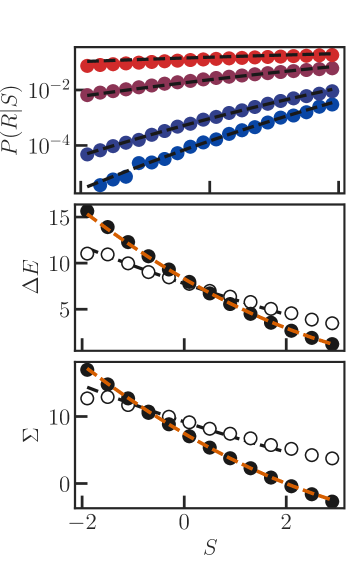
Note that each of the diagonal terms of the covariance matrix, , has the same value, , and the off-diagonal terms depend only on the distance between sites and so that . In our lattice model, we approximate the dynamics of the particulate system with a sequence of discrete “rearrangements.” These are detected in the MD simulation as events when some indicator of single-particle motion (in our case, , computed on inherent-state positions as in [23]), rises above some threshold. The probability of a particle rearranging is found, in simulation data, to depend on its softness through the Arrhenius law
| (3) |
As in [23, 28], and are roughly linear in , and deviations can be adequately treated by quadratic corrections [28] (see Fig. 1). Thus, we also have
| (4) |
with and related to the linear and quadratic coefficients in and . We assume continuous time dynamics consisting of a series of instantaneous “rearrangements” that occur with a rate proportional to the measured in MD simulations.
To formulate precisely how detailed balance constrains the distribution of for a rearrangement, we construct the distribution of given that a site at the origin is rearranging, using Bayes’ theorem:
| (5) |
Clearly, must be a normal distribution whose mean and covariance we denote by and . Direct calculation (Appendix B) shows that at a distance from the rearranging site, and for sites and at distances and from the rearranging site and with separation , are given by
| (6) | ||||
| (7) | ||||
| (8) | ||||
| (9) |
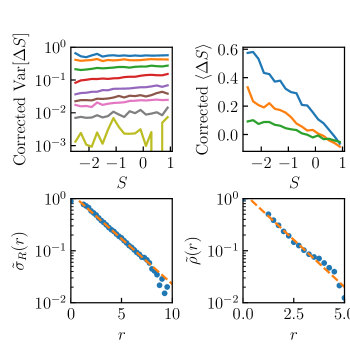
Now consider the vector , the change of softness induced by a rearrangement at the origin. We approximate the distribution of as Gaussian as well, with mean and covariance matrix . Fig. 3(b) shows that is roughly a linear function of . The covariance for two sites should decay both as they become separated from each other as well as from the rearrangement at the origin, since the effect of the rearrangement should be short-ranged. We find from MD simulations that after subtracting a background we associate with undetected rearrangements, appears to be independent of (Fig. 3(a)). Thus, we assume that is independent of . The simplest possible model therefore has the form
| (10) |
If the matrix is taken to be diagonal, this means that a rearrangement tends to restore a site’s softness toward some “target” value with some “strength” ; if has off-diagonal elements then the softness of one’s neighbor influences this mean change.
Under these assumptions, the joint distribution of the softness field before and after a rearrangement, , is Gaussian. This may be seen by explicitly writing out the density
| (11) |
using our assumed forms for all three probabilities.
In order for the system to satisfy detailed balance, the joint distributions of for all particles before and after the rearrangement must be equal:
| (12) |
Applying this constraint to a rearrangement at the origin places conditions on the distribution of : a generic distribution of will not be consistent with detailed balance between the states and . Instead of working with Eq. 12 directly, it is far easier to derive these conditions by using the fact that, as stated above, and have a joint Gaussian distribution in the case of a linear correlation between and . We construct the block covariance matrix of the random variable :
| (15) |
The fact that the rearrangement obeys time-reversal symmetry captured by the equality of the two diagonal blocks and the equality of the two off-diagonal blocks. Since a linear transformation of a Gaussian random variable with covariance and mean yields and , we may easily construct the covariance and mean of
| (16) | ||||
| (19) |
Finally, we condition on to construct (Appendix B). After identifying , this yields the conditions
| (20) | ||||
| (21) |
To understand the meaning of these conditions, consider a simple model without spatial correlations in or . In this case and , and the latter condition reduces to
| (22) |
Thus, we can see that these conditions state that the variance of the kick, , and the degree to which is “restored” toward the mean , , cannot be independent of each other. This is intuitively reasonable from time-reversibility: if the restoring term is much stronger (weaker) than the random kick, then the distribution at distance will tend to narrow (broaden) due to the rearrangement. But since the rearrangement is still at distance from the site under consideration in the time-reversed trajectory, this violates time-reversal symmetry.
If there are spatial correlations in and , then detailed balance constrains the relation between the covariance of the kick, , and the degree to which is restored to its mean, as in Eq. 21. In other words, if we measure the covariances of and in simulations, detailed balance constrains the value of . Assuming the necessary square root exists, we have the unique solution [39] 111In general the square root of a matrix is not unique—for each eigenvalue we have a choice about whether to choose the positive square root or the negative square root. However, we must always choose the positive square root; if has an eigenvalue greater than , it corresponds to an unphysical solution in which on average overshoots its equilibrium value.
| (23) |
For the square root to exist, the eigenvalues of must be less than 1; this generalizes an observation in the uncorrelated case that the variance of for the rearranging particle must not exceed the variance of the softness itself.
IV Generalizing TRSP models to multiple-particle rearrangements
In the above TRSP model, we have assumed that a single site “rearranges” at a time. This model underestimates the size of dynamical heterogeneity (see Appendix G). In reality, rearrangements must involve multiple neighbouring particles passing over the threshold ; this “rearrangement size” contributes to the measured dynamical correlations. Note that the rearrangement size is a same-time correlation; when a particle rearranges there are usually neighbours rearranging with it. Indeed, if one considers an elementary T1 event, four particles must rearrange in tandem.
We therefore generalize our rearrangement rule based on and our distribution of to allow for rearrangements composed of multiple particles. For simplicity we assume that all rearrangements involve exactly particles. Once is chosen, we consider only rearrangements involving adjacent particles. We assume that the rate of rearrangement for a cluster of particles is determined by the average of the cluster, i.e. . Furthermore, we assume that the variance of for a particle is determined by its distance from the nearest rearranging particle. These choices are the simplest one which preserve the symmetry between the rearranging particles and other basic physical considerations. In Appendix C we discuss the problems with other “obvious” choices for the multi-particle rearrangement rule.
This change in the model requires a “renormalization” of . The observed is now related to the “bare” function by an average over the neighbour softness , conditioned on a given particle’s . We carry out the necessary Gaussian integral and solve the resulting equations for the parameters of the bare in terms of the observed parameters. This calculation, sketched in Appendix D, results in
| (24) | ||||
| (25) | ||||
| (26) |
where
| (27) |
is the average correlation of between particles , in the rearranging cluster, and is the ratio between the number of clusters and the number of sites .
The question remains of how to implement the softness change produced by a multi-particle rearrangement in a manner which preserves time-reversal symmetry. To begin to address this question, we must compute the distribution of conditioned on a particular set of rearranging particles . A straightforward calculation generalizing equations 6–9 to multi-particle rearrangements (Appendix B) shows that the covariance matrix and mean are given by
| (28) | ||||
| (29) | ||||
| (30) |
where denotes the average of for every rearranging site and denotes the average over all pairs of (not necessarily distinct) rearranging sites .
We may preserve detailed balance by choosing any functional form for that treats the different rearranging sites on equal footing, using our previously-derived detailed-balance conditions 21, with the new value of in equation 23, and restoring now toward the newly-derived . Two obvious choices are a which depends only on the distance to the center of mass of the rearrangement, and our actual choice, a which depends only on the closest distance to any rearranging site.
Inspired by T1 events, we will consider the case , and specifically restrict rearrangements to clusters of particles arranged in a nearest-neighbor square (plaquette).
V Measuring TRSP model parameters from MD simulation
The model is determined by , , , , and , which we extract from simulations. Detailed balance then fixes and at each temperature.
As in [28], we assume that
| (31) | ||||
| (32) |
Here the parameter is an “onset temperature”, above which dynamics no longer depend on the structure as measured through [23]. Here we obtain this onset temperature through the best fit of to the data and obtain a noticeably lower temperature than in past work ( rather than ). The discrepancy is likely due to the wider range of considered; at high the quadratic correction to has a stronger effect. Note that we find this difference in both with and without rate renormalization.
Fig. 1(a) shows , measured in MD simulations, at several temperatures. Fig. 1(b,c) show the fit values of and (white circles), and the inferred bare values (black circles). The dashed orange lines show fits to 31 and 32. The dashed black lines in Fig. 1(a) are the result of passing the bare values of and back through equations 24-26, showing that the renormalized fit describes adequately. This confirms our choices that entered into the renormalization.
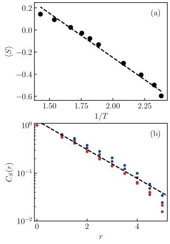
We must now fit the correlation function and the mean softness . (Note that alternatively the model could be parameterized using the at which the mean for rearranging particles is zero at each instead of .) We measure the mean (Fig. 2(a)) and correlation function (Fig. 2(b) of as a function of . is adequately approximated by an Arrhenius-like form, . We find that is well-fit by a function of the form
| (33) |
where , . The correlation length appears to grow slightly with decreasing temperature, as expected, but for now we neglect this effect and fit the correlation function at high .
All that now remains is to measure . In principle may be an arbitrary function of , . However, binning the data for rearrangements in , and the angle between them produces data which are too noisy for reliable inference of . To make progress we approximate by the factorization
| (34) |
where () is the shortest distance between () and a rearranging particle and .
First we measure , i.e. the magnitude of the softness change at distance . To do so, we look at the variance of for particles which are distance to the closest rearranging particle, over the span of that rearrangement. For each rearrangement we compare at times relative to the rearrangement. There is a small nonzero plateau of this variance as ; this plateau value is larger for particles with large . This is consistent with an interpretation of this plateau as resulting from undetected rearrangements below the threshold . We “subtract off” this effect of undetected rearrangements, as detailed in Appendix E. Doing so results in a variance which is roughly independent of at each (Fig 3(a)), as assumed above. We then average out the fluctuations over all bins, producing a numerical estimate of . We measure by measuring for rearrangements at the origin.
As shown in Fig. 3(c,d), we find that and are well fit by the almost-exponential function given by Equation 33. We assume that is independent of temperature—at high temperatures there may be many more rearrangements, but since a rearrangement is defined as a structural change of a certain magnitude, it is reasonable to assume that the effect of an individual rearrangement is roughly independent of temperature.
After determining the form of , the form of is fixed by time-reversal symmetry through Eq. 23, which we evaluate numerically. Note that since we are placing the model on a square lattice, this will in principle produce a slightly anisotropic .
We find that, at all temperatures, the average duration of a rearrangement, measured by the number of consecutive frames (separated by ) where , given that for at least one frame, is roughly . Thus, the rate of rearrangement is taken to be .
VI TRSP model calculations
After fitting the model parameters, we simulate the model on a cubic lattice of linear dimension with periodic boundary conditions. We take the lattice spacing to be equal to the first peak of the large particle-large particle pair correlation function .
We use Gillespie’s method to determine each rearrangement event in sequence[41] rather than using a fixed timestep . Multivariate Gaussian random variables are generated using a standard FFT-based technique for translation-invariant covariance matrices [42].
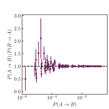
At each temperature we initialize the system with a state drawn from the equilibrium distribution . We verify that and do not change in time from the putative equilibrium values, as expected from our detailed-balance conditions (Appendix F.2). We also check explicitly that detailed balance is satisfied (Appendix F.1). Equilibrium dynamical (i.e. two-time) quantities are averaged both over time and over 20 (high ) or 40 (low ) independent initial conditions from the equilibrium distribution. Aging simulations are instead averaged over 50 independent initial conditions.
VII Comparison of TRSP model with MD simulations
VII.1 Dynamical heterogeneity
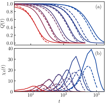
To characterize the relaxation dynamics of the model we compute the overlap function, , defined as
| (35) |
where is an indicator variable that is if particle has not rearranged and if it has.
The dynamical susceptibility is defined as
| (36) |
We define the time at which is maximized as and its peak value to be .
To test our model, we compare and to observations from MD simulations. We adopt the picture that the dynamics consists of transitions between inherent states with vibrational motion superimposed on top [43, 3]. Since our model only seeks to describe these inherent-state transitions, comparison to inherent-state or is more natural than comparison to values computed using instantaneous positions. Using instantaneous positions, for example, reduces the peak value of , which we interpret as effectively superimposing noise upon the real correlations in the dynamics.
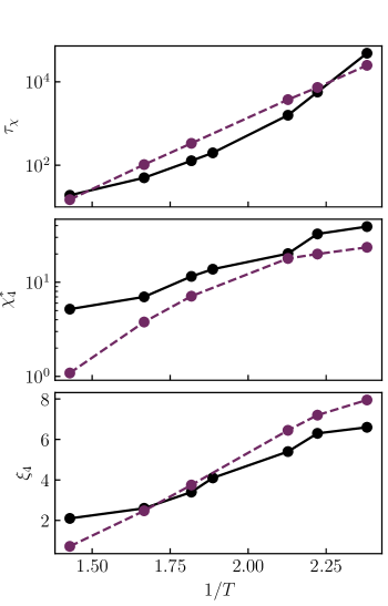
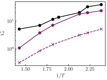
Figure 4 shows and for various temperatures , showing qualitative agreement between MD simulations (A,C) and the model (B,D). Fig 5(A,B) show and for the MD simulations and the TRSP model as a function of . The agreement between the two is quantitatively reasonable. We note, however, that the TRSP model clearly underestimates the fragility (strength of non-Arrhenius behavior in vs. ) and the overall magnitude of .
Note that with the exception of the highest temperature studied, , the scaling of with is captured well by the model. The poor performance of the model near may be related to the breakdown of the assumption that the dynamics can be well-approximated by a sequence of discrete rearrangements. Alternatively, we note that the dynamical length scale at high approaches the lattice spacing. As a result, the observed deviation from our theory may arise from a breakdown of the lattice approximation or of the assumption that all rearrangements involve particles (see below).
For reference, note that a model of nonoverlapping clusters of particles that rearrange together, each with identical rearrangement rates, would produce [28]. The fact that the clusters in our model are allowed to overlap reduces . relative to the trap prediction. Since all correlations of rearrangement rates vanish at , the rough scale of near produced by the model matches our expectations. Thus, indeed, it is clear that the we see near in the MD data is too high to be explained by this model of discrete rearrangements.
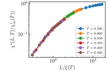
In supercooled liquids, the growth of with decreasing temperature is associated with growth of a dynamical correlation length , which can become quite large at low temperatures. Since we have not included any growth of either the softness correlation length or the size of rearrangements in the model, it is not obvious that such a growing length scale is the origin of the growth of in our model. To investigate this, we measure in both the TRSP model and MD simulations.
In each case, we measure at a single high temperature by fitting the dynamical structure factor , defined by
| (37) | ||||
| (38) |
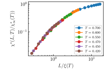
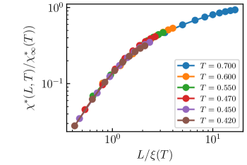
evaluated at , to an Ornstein-Zernicke form [44, 45], and then measure the growth of with cooling by performing a finite-size scaling collapse of measured in subsystems of varying size [46].
The result of this calculation is shown in Fig. 5(c). We see that, in fact, this model does predict a dynamical length that grows with decreasing , even though we have not included growth in the static length scale.
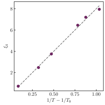
How can the growing dynamical correlations originate from a fixed static length scale ? Intuitively, this is because a given difference in results in a bigger difference in rearrangement rates at lower ; thus, the same static correlations “count for more” at lower .
More precisely, the contribution of to is proportional to . Thus, in Fig. 6 we plot in our model as a function of . We find the relationship between the two to be nearly linear, supporting the picture that the dynamical length in this model comes, roughly speaking, from multiplying the static correlation length by this growing contribution of to the probability of rearrangement.
VII.2 Correlation vs. causation in TRSP model
We now turn to the origin of the growing dynamical correlations with decreasing within the TRSP model.
We can imagine three possible origins for the dynamics correlations in the model:
-
1.
The constraint that particles rearrange in groups of .
-
2.
Spatial correlations in (correlation).
-
3.
Facilitation, or causation ( induced by rearrangements)
The first factor could be labeled as causation but really just accounts for the reality that a rearrangement involves more than one particle. It certainly makes a contribution—the single-site rearrangement version of the TRSP model produces a much smaller value of at all temperatures (see Appendix G). However, although this affects the magnitude, it does not affect the temperature-dependence significantly. We therefore focus on the second and third effects.
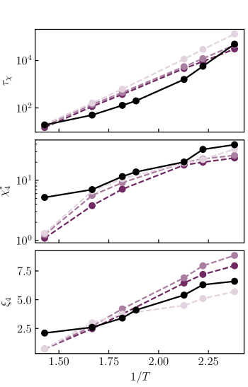
One virtue of the TRSP model is that the contributions of correlation and causation to dynamical heterogeneity are transparent. To investigate the relative roles of (2) and (3), we take advantage of our explicit conditions for guaranteeing time-reversal symmetry to generate alternate models. Using the detailed-balance conditions, we can construct a more general model in which the variance of for all particles is reduced by a factor , while holding the spatial correlations of fixed. Thus, the contribution to from static spatial correlations in mobility is held fixed, but the effect of rearrangements on future mobility (facilitation) is weakened–correlation is held fixed by causation is reduced by a factor . The result of this analysis is shown in Fig. 7. Evidently, weakening facilitation in this model increases both and . Thus, it appears that the growth of dynamical correlations in this model arises from the static softness correlations , and facilitation (that is, changes in induced by rearrangements) only reduces .
The fact that facilitation lowers may seem surprising at first but is intuitively plausible. Recall that facilitation must satisfy detailed balance. Thus, despite what one might imagine from the word “facilitation”, it is just as likely to make a neighboring particle less soft as it is to make it softer. One can imagine that the effect of facilitation on depends on temperature. At sufficiently high , the neighbor of a soft particle is likely already soft due to the equilibrium spatial correlations. Indeed, it is likely soft enough to rearrange with high probability, even without facilitation. If faciltation lowers its softness, however, it will weaken the dynamical effects of the correlation present in the initial structure.
From this reasoning, it seems plausible that the sign of the effect may change at low enough , when the average softness is lower and so that particles are unlikely to rearrange even if they are soft. In this case, lowering of nearby particles may effectively make no difference, while raising it may allow an avalanche to propagate. Indeed, Figure 7(c) shows that weakening facilitation actually lowers at low , and in the finite-size collapse (Appendix H, Figure 16), the extrapolation of to infinite system size actually decreases at for low (data not shown). Thus, at low , it is possible that TRSP calculations for larger systems (which could be achieved by modifying the code to cut off the change in beyond a certain range) may show a crossover in the effect of facilitation on . Similarly, finite size effects may contribute to the lack of fragility observed, since the finite system size will cut off the growth of due to growth of mobile domains when their size becomes comparable to the system size.
VII.3 Aging
We next investigate the behavior of our model during aging. Although detailed balance is not satisfied out-of-equilibrium, this does not preclude using our model to study aging—indeed, the true dynamics do not satisfy detailed balance out of equilibrium, but crucially, out of equilibrium MD is still governed by the same dynamical equations as in equilibrium. Aging should still be described by dynamical equations which satisfy detailed balance once the steady state is reached.
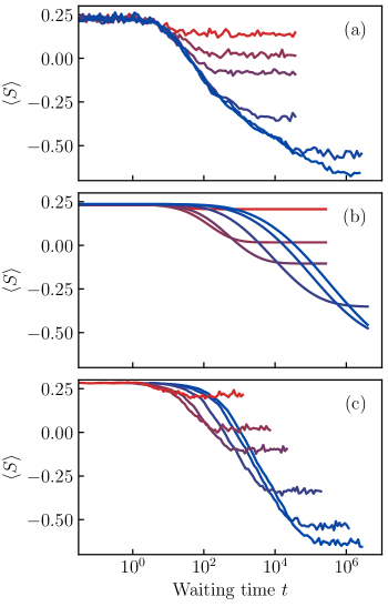
In the MD simulations, the aging dynamics of as a function of waiting time show a remarkable phenomenon: for samples quenched from the same high temperature to different final temperatures , , is the same at intermediate times (Fig. 8(a) and [14]).
This collapse cannot be reproduced by a model without interactions between particles [28]. Intuitively, this is because, if is the same at some time for different quench temperatures , then the colder temperature will have slower aging dynamics and thus the curves must separate as increases.
We modified the trap-like, independent particle model of [28] to have a -dependent density of traps, in order to produce the correct distribution of at every . We then simulate aging in this model, showing in (8(b)). We find that it still fails to produce the collapse of during aging which is observed in MD data. Thus, the trap model cannot reproduce the observed MD behavior.
The same calculations of can be carried out on the TRSP model during aging (Fig. 8(c)). We find that including interactions between sites as in the TRSP model still fails to reproduce the collapse of at intermediate times seen in the MD data (Fig. 8(a)). However, the different curves are much closer together than in the trap model, suggesting that perhaps the interactions between sites are not sufficiently strong in the TRSP model.
VIII Discussion
VIII.1 Underestimation of fragility and
We now consider possible explanations for why the TRSP model underestimates fragility and . Past work explaining empirically using softness [23] included two corrections that we have neglected here. First, they measured the fraction of rearrangements that involve a displacement greater than the threshold used to compute at each , and corrected the prediction by this factor. Secondly, they measured the fraction of rearrangements that reverse themselves at each , and corrected the prediction by this factor. Both of these corrections have the effect of increasing at low , while having little effect at high . Thus, they tend to increase fragility. We could have included these effects but chose not to, in order to present the model in its simplest form.
Another likely reason for the underestimation of fragility and is the shortcoming of as a structural descriptor. More complex machine learning methods produce structural descriptors that correlate more strongly with long-time dynamics than the linear method used to define [47, 48, 49, 50]. If such methods are optimized to predict short-time rather than long-time dynamics, they would presumably result in stronger dependencies of and on the descriptors, increasing both the degree of heterogeneity and fragility produced by the model. Indeed, the range of and produced by a structural descriptor is likely to be a good indicator of the quality of that descriptor. For example, the structural variable constructed using a neural network in [47] seems to correlate extremely well with dynamical heterogeneity and could be a better short-time descriptor than softness. (Note, however, that the reconstructed in that work using their structural variable is not the same as our , as it neglects certain kinds of dynamical fluctuations.)
These considerations point to the importance of testing the Arrhenius dependence for for structural descriptors besides softness. A TRSP-type model could be constructed using any scalar descriptor of structure. All that is required is that the dependence of the probability of rearrangement is Arrhenius for particles with a given value of the structural descriptor, and the distribution of values of the descriptor is reasonably Gaussian. This is why we regard the TRSP approach as a general framework for constructing time-reversal-invariant structuro-plasticity models.
A third contributing factor is that we have only included the effects of rearrangements of large particles in our binary system on other particles. The particles belong in the majority, but rearrangements of small particles are actually more numerous, especially as decreases, and can facilitate rearrangements of both and particles.
Finally, recall that there is evidence that the range of spatial correlations of increases with with decreasing . Such an increase would presumably also lead to greater fragility and larger values of .
VIII.2 The role of elasticity
As noted in the introduction, we have neglected elastic (far-field) facilitation. On timescales much shorter than one expects the supercooled liquid to behave as a solid (as indeed glasses do when observed out of equilibrium). Furthermore the inherent state is, by construction, a forced-balanced state and therefore perturbations around it should be described on long length scales by continuum elasticity. Recent work has demonstrated clear anisotropies in the correlated dynamics of supercooled liquids below the mode-coupling crossover temperature , which provide evidence that at least some facilitation arises from elasticity at sufficiently low temperatures [32]. Thus at low we expect that this model should pick up terms which make it resemble in spirit a thermal elastoplastic model with a softness kernel in addition to an elastic kernel, in a manner similar to [33, 34, 35].
It is not entirely obvious whether or not far-field elastic facilitation should increase or decrease . On one hand, on short timescales, elastic facilitation, by pushing neighbors over their thresholds simultaneously, effectively acts like our “multi-particle rearrangements” (), which should increase . On the other hand, elastoplasticity also produces a long-time facilitation effect, which in our current model tends to decrease . Thus the net effect of elastoplasticity on is unclear. On the empirical side, recent very-low simulations of the Kob-Andersen Lennard-Jones system appear to display a strong-to-fragile crossover with a slowing growth of at low , which could be consistent with elastoplastic-facilitation-weakened heterogeneity [51].
Recently, a simple thermal EPM has been studied as an explanation of dynamical heterogeneity [52]. In this model, which does not include near-field structural facilitation, elastic facilitation alone is found to produce a growth of with decreasing temperature. However, there are two factors which make it unclear how this result will generalize to more realistic models. First, because this model reduces to the trivial “trap” limit of uncorrelated sites when elasticity is removed, cannot, by construction, decrease when elasticity is incorporated222We do not have a rigorous proof of this fact, but it seems very likely that the case of uncorrelated, identical barriers provides a lower bound on the degree of dynamical correlation.. Second, the thermal EPM [52] does not respect detailed balance. As we have argued in section VII.2, our observation that facilitation decreases seems to be intimately connected to detailed balance, and indeed it is intuitively obvious that if for some particular were strictly positive then it would increase the degree of dynamical correlation. Put differently, while one may interpret Ref. [52] as showing that elastoplastic facilitation increases , it is doing so with the spatial correlations of the barriers not held fixed, but instead being allowed to increase by the introduction of elasticity. Note, however, that it has been argued that the origin of the dynamic length scale in these models is a “nucleation and growth” process rather than any spatial correlations of barriers [54]. It would be extremely interesting to investigate these questions in a thermal EPM that respects time-reversal symmetry.
Another recent model, composed of discrete excitations interacting elastically, very naturally respects time reversal symmetry, and may suggest an alternate route to adding elastic interactions to our model, as well as another model in which to study the effects of facilitation on [55].
As noted in [52], however, it remains true that dynamic heterogeneity with similar phenomenology is observed in systems outside of thermal equilibrium, e.g. granular systems [56, 57]. Thus, although the details of how e.g. facilitation contributes to dynamical heterogeneity may depend on time-reversal symmetry as we have argued, the basic phenomenolgy must remain. It is unclear what principles may be used to constrain our models of the dynamics of when we depart from thermal equilibrium.
IX Acknowledgements
We thank Rahul Chacko, Indrajit Tah, Richard Stephens, Misaki Ozawa, Muhammad Hasyim, and Matthieu Wyart for helpful discussions. This work was supported by the Simons Foundation via the “Cracking the glass problem” collaboration (#454945, SAR and AJL), and Simons Investigator awards to AJL (#327939) and to Ilya Nemenman (SAR). AJL thanks CCB at the Flatiron Institute, as well as the Isaac Newton Institute for Mathematical Sciences under the program “New Statistical Physics in Living Matter” (EPSRC grant EP/R014601/1), for support and hospitality while a portion of this research was carried out.
Appendix A Structure functions used to construct softness
We use the same structure functions as in [28]. These are the same as those used in [21, 23, 14], but with more radial structure functions. We use the radial structure functions
| (39) |
We take , , and
We also use the angular structure functions
| (40) |
with , , and taking combinations of values, as in [21].
Appendix B Details of detailed-balance condition derivation
As stated in the main text we consider a lattice model, where the vector contains the softness of each site. We assume that at equilibrium is drawn from a multivariate normal distribution, with a covariance matrix , i.e.
| (41) |
The probability of a particle rearranging depends on its softness through
| (42) |
where the temperature dependence of the coefficients is Arrhenius. The correction term is small.
To determine how detailed balance constrains the distribution of for a rearrangement, we write down the distribution of given that a particle at the origin is rearranging:
| (43) |
a normal distribution whose covariance we denote . Taking the logarithm of both sides of this equation (note that the quantities inside the exponentials are just real numbers) yields (with an arbitrary constant, and the vector with a at site and zeros elsewhere):
| (44) | ||||
| (45) | ||||
| (46) |
Now introduce the covariance matrix of rearranging particles, , and write
| (47) | ||||
| (48) |
We then immediately read off the mean softness at distance from a rearranging particle, and use the Sherman-Morrison formula to compute . This gives us the mean softness at a distance from a rearranging particle, and , as
| (49) | ||||
| (50) |
Now we assume that is Gaussian with mean
| (51) |
and covariance .
In the main text we asserted that this assumption gives a distribution of which is Gaussian. To see this, write
| (52) | ||||
| (53) | ||||
| (54) |
What appears inside the exponential is a quadratic form in the vector and thus the joint distribution is Gaussian. As sketched in the main text we will make use of this fact to facilitate our derivation of the detailed-balance conditions. We use the fact that and have a joint Gaussian distribution in the case of a linear correlation between and , and describe this joint distribution by the block covariance matrix of the random variable :
| (57) |
The fact that the rearrangement obeys time-reversal symmetry is expressed in the equality of the diagonal and off-diagonal blocks. Since a linear transformation of a Gaussian random variable with covariance and mean yields and , we construct the covariance and mean of
| (58) | ||||
| (61) |
Finally, we condition on to construct . For with a joint Gaussian distribution, it is known that is Gaussian with covariance and mean . Thus, is Gaussian with
| (62) | ||||
| (63) | ||||
| (64) | ||||
| (65) | ||||
| (66) | ||||
| (67) |
which this yields the conditions
| (68) | ||||
| (69) |
as claimed in the main text. As stated in the main text, satisfying this equation is given by Equation 23.
Working directly with detailed balance instead, after a substantial amount of algebra, yields the condition
| (70) |
given by Equation 23 (i.e. the solution to equation 69) also solves equation 70. This follows from the fact that this solution is of the form for an analytic function . By expanding in series and using the symmetry of and we may show that is a symmetric matrix for any analytic ; with this fact it is straightforward to manipulate equation 70 to be the same as equation 69.
Appendix C Choice of multi-site rearrangement rule
To generalize the observed and into a rule for multi-body rearrangements we must satisfy two criteria:
-
1.
The size of elementary rearrangements should be independent of , or perhaps weakly dependent on . In particular elementary rearrangements should not involve times as many particles just because the relaxation time is times shorter.
-
2.
Time-reversal symmetry should remain satisfied for
-
3.
Ideally, the different particles participating in the rearrangement should be treated in the exact same way. At the very least, the identity of all rearranging particles should affect , to preserve dynamical correlations.
The most obvious way to satisfy condition 3 is to simply make the probability of a multi-particle rearrangement involving particles equal to This, however, runs afoul of condition 1: it will produce single-particle rearrangements at low temperatures and many-particle rearrangements at high temperatures.
This naturally leads us to consider rules where the “secondary” rearrangements is not involved in the probability of rearrangement—i.e. the rearrangement of a “soft” particle can easily force a “hard” neighbor to go along with it.
The simplest way to get a rule which satisfies condition 2 and 1 is to simply determine a “primary” rearranging particle according to , determine simultaneous “secondary” rearranging particles according to some other rule, and only use the primary rearranging particle to determine . This is the approach of reference [35]. This is, however, a strong violation of condition 3.
One other idea, then, is to trigger secondary rearrangements with a softness-independent probability as in reference [35], but then allow each of these secondary rearrangements to produce some . This still does not give full permutation symmetry between the different rearranging particles (the “primary rearrangement”) is singled out), but would still preserve some dynamical correlations caused by which rearranging neighbour rearranges. It is difficult, however, to ensure that such a scheme truly satisfies time-reversal symmetry. In such a scheme, the simultaneous rearrangement of particles and can proceed by one of two “pathways”: one dependent on and one dependent on . If we assume that these two different processes produce the same distribution of then the equations of detailed balance become analytically intractable. On the other hand, if we assume the two processes have different distributions of we find that full symmetry between the two single-particle rearrangements still cannot be restored: in order to satisfy detailed balance the distribution of for the two rearrangements must be different.
The simplest rule which satisfies all the conditions is to use the average of the rearranging sites in order to determine the probability of a rearrangement. The disadvantage of this rule, however, is that it offers no insight into what sets the size of elementary rearrangements: we must put the distribution of rearrangement sizes in by hand, and in our case we choose to fix the size.
We then must fix the distribution of in order to satisfy condition 2. Using the average still permits this as it keeps Gaussian; a rearrangement probability which is exponential in any second-order polynomial of will work. One might hope that there is a straightforward way to “build” the distribution of by the successive action of two single-particle rearrangements. If there was a method which allowed use to think of the two rearrangements as “simultaneous” (e.g. if had a distribution which was independent of the order of rearrangements) then we could proceed as such. One finds however, that the distribution of in such a case depends on the order of the rearrangements. Thus, if we wish to satisfy time-reversal symmetry we require the rearrangement “particle rearranges, then particle rearranges” to proceed by two independent pathways, one determined by and one by , with no reference at all to the ordering of the rearrangements. Thus, the most straightforward approach is to construct with no reference to hypothetical single-particle rearrangements, e.g. by assuming it is a function of distance from the center of mass of the rearrangement, or from the set of all rearranging particles as we have done.
Appendix D Renormalization of for multi-site rearrangements
As in the main text, assume that each group of neighbouring sites rearranges with a probability
| (71) |
for some “bare” rate . The apparent rearrangement rate for each particle is thus
| (72) |
where is the number of clusters of size we consider for rearrangement that contain a given site (e.g. and on a cubic lattice).
We note that the conditional distribution is Gaussian. Its covariance is , and its mean is .
Doing the Gaussian integral yields the observed in terms of the bare parameters. The result is of the form
| (73) |
with the “renormalized” parameters determined by the “bare” parameters . The set of equations relating them may be solved to obtain , and . This produces the equations in the main text.
Appendix E Subtracting off the background from measurements of and
As mentioned in the main text, we interpret the values of and as in the MD data as a background value caused by undetected rearrangements. Here we explain in detail how the background events are subtracted off.
Intuitively, if we imagine that the observed is a sum of two processes, and , we might suppose that we can take advantage of the linearity of the mean and variance, to write and . Thus, we could obtain the parameters for the rearrangement by subtracting off the background. This produces results which look reasonable at long distances and low temperatures, but it cannot be consistent if is too large (it is unphysical to have .)
In reality, and cannot be assumed to be uncorrelated, since the mean is correlated with . If we assume a gaussian distribution of and do the integral over the possible values of , then substitute in the approximate (uncorrelated) detailed balance condition 22, we arrive at the corrected sum formulae
| (74) | ||||
| (75) |
These formulae are used to subtract off the background in Fig. 3.
In the above, we have ignored the effect of spatial correlations in and the covariance structure of , under the assumption that this is sufficient for measuring the approximate magnitude of . Note that, as discussed in section C, if we wish to go beyond this approximation the idea of “adding together” the effect of multiple rearrangements becomes poorly defined, with the result depending on the ordering of the rearrangements.
Appendix F Tests of model implementation
F.1 Direct test of detailed balance
In equilibrium the model is constructed to satisfy detailed balance, i.e. for any .
Detailed balance is preserved by any coarsening of the state space, i.e. a mapping from to in some discrete space. Thus, we may directly test detailed balance in our model simulations by letting represent the binned value of for a rearranging particle, and then checking that .
Figure 9 shows the results of this test, plotting against for the numerical simulation of the model at . For this coarsening of the states, detailed balance is satisfied within error bars.
F.2 Mean and correlation functions of
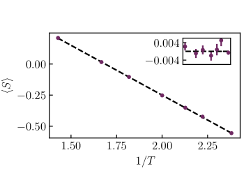
The model is constructed to reproduce a known and correlation function ; we also verify this in our numerical implementation of the model.
Some care is required to precisely compute any such average over the distribution of . The samples produced by the Gillespie algorithm are of rearrangement events, and are thus biased toward their values for rearranging particles by fluctuations in of order . To do proper time averaging, the samples obtained must be weighted by the time until the next rearrangement event.
Figure 10 shows the simulated as a function of the theoretical for the used parameters, showing perfect agreement. Figure 11 shows the correlation function at alongside the target function, again showing perfect agreement. The same plot for other simulated temperatures (not shown) shows the same result, and the small deviations from the target correlation function do not show any systematic trend with temperature .

Appendix G A model with single-site rearrangements strongly underestimates
As stated in the main text, we decided assume rearrangements involve particles after observing that a model without this effect strongly underestimates the value of . Figure 12 compares the produced by such a model to the values for MD data and our full model, as shown in Figure 5.
Appendix H Scaling collapses to extract
As in [46], we extract the scaling of by scaling collapse of computed for subsystems (“blocks”) of size . These collapses are shown in 13 and 14.

References
- [1] Andrea Cavagna. Supercooled liquids for pedestrians. Physics Reports, 476(4-6):51–124, 2009.
- [2] C. A. Angell. Formation of Glasses from Liquids and Biopolymers. Science, 267(5206):1924–1935, 1995.
- [3] Srikanth Sastry, Pablo G. Debenedetti, and Frank H. Stillinger. Signatures of distinct dynamical regimes in the energy landscape of a glass-forming liquid. Nature, 393(6685):554–557, 1998.
- [4] Pablo G. Debenedetti and Frank H. Stillinger. Supercooled liquids and the glass transition. Nature, 410(6825):259–267, 2001.
- [5] Ludovic Berthier Giulio Biroli (ed.), Jean-Philippe Bouchaud (ed.), Luca Cipelletti, Wim van Saarloos (ed.), and Giulio Biroli, editors. Dynamical Heterogeneities in Glasses, Colloids, and Granular Media. Oxford University Press, 2011.
- [6] M. D. Ediger. Spatially Heterogeneous Dynamics in Supercooled Liquids. Annual Review of Physical Chemistry, 51(1):99–128, 2000.
- [7] Walter Kob, Claudio Donati, Steven J. Plimpton, Peter H. Poole, and Sharon C. Glotzer. Dynamical Heterogeneities in a Supercooled Lennard-Jones Liquid. Physical Review Letters, 79(15):2827–2830, 1997.
- [8] E. Vidal Russel and N. E. Israeloff. Direct observation of molecular cooperativity near the glass transition. Nature, 408(6813):695–698, 2000.
- [9] M. D. Ediger, C. A. Angell, and Sidney R. Nagel. Supercooled Liquids and Glasses. The Journal of Physical Chemistry, 100(31):13200–13212, 1996.
- [10] C. A. Angell, K. L. Ngai, G. B. McKenna, P. F. McMillan, and S. W. Martin. Relaxation in glassforming liquids and amorphous solids. Journal of Applied Physics, 88(6):3113–3157, 2000.
- [11] Walter Kob and Jean-Louis Barrat. Aging Effects in a Lennard-Jones Glass. Physical Review Letters, 78(24):4581–4584, 1997.
- [12] W. Kob and J.-L. Barrat. Fluctuations, response and aging dynamics in a simple glass-forming liquid out of equilibrium. The European Physical Journal B - Condensed Matter and Complex Systems, 13(2):319–333, 2000.
- [13] Jörg Rottler and Mark O. Robbins. Unified Description of Aging and Rate Effects in Yield of Glassy Solids. Physical Review Letters, 95(22):225504, 2005.
- [14] Samuel S. Schoenholz, Ekin D. Cubuk, Efthimios Kaxiras, and Andrea J. Liu. Relationship between local structure and relaxation in out-of-equilibrium glassy systems. Proceedings of the National Academy of Sciences, 114(2):263–267, 2017.
- [15] Jeppe C. Dyre. Colloquium: The glass transition and elastic models of glass-forming liquids. Reviews of Modern Physics, 78(3):953–972, 2006.
- [16] Asaph Widmer-Cooper, Peter Harrowell, and H. Fynewever. How Reproducible Are Dynamic Heterogeneities in a Supercooled Liquid? Physical Review Letters, 93(13):135701, 2004.
- [17] John J Gilman. Metallic glasses. Physics Today, 28(5):46–53, 1975.
- [18] Robert L. Jack, Andrew J. Dunleavy, and C. Patrick Royall. Information-Theoretic Measurements of Coupling between Structure and Dynamics in Glass Formers. Physical Review Letters, 113(9):095703, 2014.
- [19] P. Chaudhari, A. Levi, and P. Steinhardt. Edge and Screw Dislocations in an Amorphous Solid. Physical Review Letters, 43(20):1517–1520, 1979.
- [20] C. Patrick Royall, Stephen R. Williams, Takehiro Ohtsuka, and Hajime Tanaka. Direct observation of a local structural mechanism for dynamic arrest. Nature Materials, 7(7):556–561, 2008.
- [21] E. D. Cubuk, S. S. Schoenholz, J. M. Rieser, B. D. Malone, J. Rottler, D. J. Durian, E. Kaxiras, and A. J. Liu. Identifying Structural Flow Defects in Disordered Solids Using Machine-Learning Methods. Physical Review Letters, 114(10):108001, 2015.
- [22] Ekin D. Cubuk, Samuel S. Schoenholz, Efthimios Kaxiras, and Andrea J. Liu. Structural Properties of Defects in Glassy Liquids. The Journal of Physical Chemistry B, 120(26):6139–6146, 2016.
- [23] S. S. Schoenholz, E. D. Cubuk, D. M. Sussman, E. Kaxiras, and A. J. Liu. A structural approach to relaxation in glassy liquids. Nature Physics, 12(5):469–471, 2016.
- [24] Ekin D. Cubuk, Andrea J. Liu, Efthimios Kaxiras, and Samuel S. Schoenholz. Unifying framework for strong and fragile liquids via machine learning: a study of liquid silica. arXiv, 2020.
- [25] Jason W. Rocks, Sean A. Ridout, and Andrea J. Liu. Learning-based approach to plasticity in athermal sheared amorphous packings: Improving softness. APL Materials, 9(2):021107, 2021. pub.
- [26] Sean A. Ridout, Jason W. Rocks, and Andrea J. Liu. Correlation of plastic events with local structure in jammed packings across spatial dimensions. Proceedings of the National Academy of Sciences, 119(16):e2119006119, 2022. pub.
- [27] Indrajit Tah and Smarajit Karmakar. Kinetic fragility directly correlates with the many-body static amorphous order in glass-forming liquids. Physical Review Materials, 6(3):035601, 2022.
- [28] S. A. Ridout, I. Tah, and A. J. Liu. Building a “trap model” of glassy dynamics from a local structural predictor of rearrangements. Europhysics Letters, 144(4):47001, 2023. pub.
- [29] David Chandler and Juan P. Garrahan. Dynamics on the Way to Forming Glass: Bubbles in Space-Time. Annual Review of Physical Chemistry, 61(1):191–217, 2010.
- [30] Anaël Lemaître. Structural Relaxation is a Scale-Free Process. Physical Review Letters, 113(24):245702, 2014.
- [31] Alexandre Nicolas, Ezequiel E. Ferrero, Kirsten Martens, and Jean-Louis Barrat. Deformation and flow of amorphous solids: Insights from elastoplastic models. Reviews of Modern Physics, 90(4):045006, 2018.
- [32] Rahul N. Chacko, François P. Landes, Giulio Biroli, Olivier Dauchot, Andrea J. Liu, and David R. Reichman. Elastoplasticity Mediates Dynamical Heterogeneity Below the Mode Coupling Temperature. Physical Review Letters, 127(4):048002, 2021.
- [33] Ge Zhang, Sean A. Ridout, and Andrea J. Liu. Interplay of Rearrangements, Strain, and Local Structure during Avalanche Propagation. Physical Review X, 11(4):041019, 2021. pub.
- [34] Ge Zhang, Hongyi Xiao, Entao Yang, Robert J. S. Ivancic, Sean A. Ridout, Robert A. Riggleman, Douglas J. Durian, and Andrea J. Liu. Structuro-elasto-plasticity model for large deformation of disordered solids. Physical Review Research, 4(4):043026, 2022. pub.
- [35] Hongyi Xiao, Ge Zhang, Entao Yang, Robert Ivancic, Sean Ridout, Robert Riggleman, Douglas J. Durian, and Andrea J. Liu. Identifying microscopic factors that influence ductility in disordered solids. Proceedings of the National Academy of Sciences, 120(42):e2307552120, 2023. pub.
- [36] R. Candelier, O. Dauchot, and G. Biroli. Building Blocks of Dynamical Heterogeneities in Dense Granular Media. Physical Review Letters, 102(8):088001, 2008.
- [37] R. Candelier, A. Widmer-Cooper, J. K. Kummerfeld, O. Dauchot, G. Biroli, P. Harrowell, and D. R. Reichman. Spatiotemporal Hierarchy of Relaxation Events, Dynamical Heterogeneities, and Structural Reorganization in a Supercooled Liquid. Physical Review Letters, 105(13):135702, 2010.
- [38] D. Richard, M. Ozawa, S. Patinet, E. Stanifer, B. Shang, S. A. Ridout, B. Xu, G. Zhang, P. K. Morse, J.-L. Barrat, L. Berthier, M. L. Falk, P. Guan, A. J. Liu, K. Martens, S. Sastry, D. Vandembroucq, E. Lerner, and M. L. Manning. Predicting plasticity in disordered solids from structural indicators. Physical Review Materials, 4(11):113609, 2020. pub.
- [39] G.L. Shurbet, T.O. Lewis, and T.L. Boullion. Quadratic Matrix Equations. Ohio Journal of Science, 1974.
- [40] In general the square root of a matrix is not unique—for each eigenvalue we have a choice about whether to choose the positive square root or the negative square root. However, we must always choose the positive square root; if has an eigenvalue greater than , it corresponds to an unphysical solution in which on average overshoots its equilibrium value.
- [41] Daniel T Gillespie. A general method for numerically simulating the stochastic time evolution of coupled chemical reactions. Journal of Computational Physics, 22(4):403–434, 1976.
- [42] Dirk P. Kroese and Zdravko I. Botev. Spatial Process Simulation. In Volker Schmidt, editor, Stochastic Geometry, Spatial Statistics, and Random Fields: Models and Algorithms. Springer Cham, 2015.
- [43] Cécile Monthus and Jean-Philippe Bouchaud. Models of traps and glass phenomenology. Journal of Physics A: Mathematical and General, 29(14):3847, 1996.
- [44] Smarajit Karmakar, Chandan Dasgupta, and Srikanth Sastry. Analysis of Dynamic Heterogeneity in a Glass Former from the Spatial Correlations of Mobility. Physical Review Letters, 105(1):015701, 2010.
- [45] Elijah Flenner and Grzegorz Szamel. Dynamic Heterogeneity in a Glass Forming Fluid: Susceptibility, Structure Factor, and Correlation Length. Physical Review Letters, 105(21):217801, 2010.
- [46] Saurish Chakrabarty, Indrajit Tah, Smarajit Karmakar, and Chandan Dasgupta. Block Analysis for the Calculation of Dynamic and Static Length Scales in Glass-Forming Liquids. Physical Review Letters, 119(20):205502, 2017.
- [47] Gerhard Jung, Giulio Biroli, and Ludovic Berthier. Predicting Dynamic Heterogeneity in Glass-Forming Liquids by Physics-Inspired Machine Learning. Physical Review Letters, 130(23):238202, 2023.
- [48] V. Bapst, T. Keck, A. Grabska-Barwińska, C. Donner, E. D. Cubuk, S. S. Schoenholz, A. Obika, A. W. R. Nelson, T. Back, D. Hassabis, and P. Kohli. Unveiling the predictive power of static structure in glassy systems. Nature Physics, 16(4):448–454, 2020.
- [49] Emanuele Boattini, Frank Smallenburg, and Laura Filion. Averaging Local Structure to Predict the Dynamic Propensity in Supercooled Liquids. Physical Review Letters, 127(8):088007, 2021.
- [50] Rinske M. Alkemade, Frank Smallenburg, and Laura Filion. Improving the prediction of glassy dynamics by pinpointing the local cage. The Journal of Chemical Physics, 158(13):134512, 2023.
- [51] Pallai Das and Srikanth Sastry. Crossover in dynamics in the Kob-Andersen binary mixture glass-forming liquid. Journal of Non-Crystalline Solids: X, 2022.
- [52] Misaki Ozawa and Giulio Biroli. Elasticity, Facilitation, and Dynamic Heterogeneity in Glass-Forming Liquids. Physical Review Letters, 130(13):138201, 2023.
- [53] We do not have a rigorous proof of this fact, but it seems very likely that the case of uncorrelated, identical barriers provides a lower bound on the degree of dynamical correlation.
- [54] Ali Tahaei, Giulio Biroli, Misaki Ozawa, Marko Popović, and Matthieu Wyart. Scaling Description of Dynamical Heterogeneity and Avalanches of Relaxation in Glass-Forming Liquids. arXiv, 2023.
- [55] Muhammad R Hasyim and Kranthi K Mandadapu. Emergent Facilitation and Glassy Dynamics in Supercooled Liquids. arXiv, 2023.
- [56] Aaron S. Keys, Adam R. Abate, Sharon C. Glotzer, and Douglas J. Durian. Measurement of growing dynamical length scales and prediction of the jamming transition in a granular material. Nature Physics, 3(4):260–264, 2007.
- [57] A. R. Abate and D. J. Durian. Topological persistence and dynamical heterogeneities near jamming. Physical Review E, 76(2):021306, 2007.