Information scrambling in quantum-walks
Abstract
We study information scrambling — a spread of initially localized quantum information into the system’s many degree of freedom — in discrete-time quantum walks. We consider out-of-time-ordered correlators (OTOC) and K-complexity as probe of information scrambling. The OTOC for local spin operators in all directions has a light-cone structure which is “shell-like”. As the wavefront passes, the OTOC approaches to zero in the long-time limit, showing no signature of scrambling. The introduction of spatial or temporal disorder changes the shape of the light-cone akin to localization of wavefuction. We formulate the K-complexity in system with discrete-time evolution, and show that it grows linearly in discrete-time quantum walk. The presence of disorder modifies this growth to sub-linear. Our study present interesting case to explore many-body phenomenon in discrete-time quantum walk using scrambling.
I Introduction
Quantum scrambling [1, 2] is the process where interactions within a quantum system spread local information across its many degree of freedom. It’s a fundamental process behind how isolated quantum systems reach thermal equilibrium [3, 4, 5], and it’s closely linked to quantum chaos [6], the black-hole information problem [7, 8, 9], and how disorder affects collective spins in many-body systems [10, 11]. The concept of scrambling also lays the groundwork for developing algorithms in quantum benchmarking and machine learning, which can make the exploration of Hilbert spaces more efficient [12, 13, 14, 15, 16].
There remain ambiguity is describing the process of quantum scrambling. One method to probe it involves using an out-of-time-ordered correlator [17, 1]. For systems that exhibit a semi-classical limit or have a large number of local degrees of freedom, this correlator shows exponential growth, which can be used to identify a quantum counterpart to the Lyapunov exponent (LE), thus linking it to classical chaos [18]. Another approach involves studying the evolution dynamics of operators in Krylov space. Here, operator growth is measured by the “K-complexity”, indicating the extent of delocalization of initial local operators evolving under Heisenberg evolution under the system Hamiltonian [19, 20, 21]. It is speculated that this K-complexity grows exponentially in most generic nonintegrable systems [19]. This exponential growth in K-complexity can be used to extract LE, establishing a connection with out-of-time-ordered correlators [6]. Recent studies have explored K-complexity in various systems such as Ising models [22, 23, 24], Sachdev-Ye-Kitaev (SYK) models [25, 26, 27], quantum field theories [28, 29, 30, 31, 32, 33], many-body localization system [34, 35], and open quantum systems [36, 37, 38, 39, 40].
Experimentally tunable toy models serve as valuable tools for investigating different phenomena from theoretical physics. One such tool, which we will pursue in this work, is the quantum walk — a quantum version of the classical random walk [41, 42]. Specifically, we examine discrete-time quantum walks, which have been previously employed to simulate controlled dynamics in quantum systems [43, 44, 45] and to construct quantum algorithms [42]. These quantum walks are implemented experimentally using both lattice-based quantum systems and circuit-based quantum processors [46, 47, 48]. The adaptability of quantum walks, allowing for the experimental modeling of various phenomena like topological effects [45, 49], therefore, also positions them as a promising platform for studying scrambling.
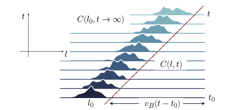
In this article, we study the out-of-time-ordered correlator (OTOC) and K-complexity for different operators in the exactly-solvable one-dimensional discrete-time quantum walk. Our study of OTOC for different spin operators shows universal “shell-like” structure so as the wavefront passes, the OTOC goes to zero in the long-time limit, in other words, operator has no support on the site, implying absence of scrambling (See Fig. 1). On the other hand, we show that K-complexity grows linearly in time, akin to approximate orthonorgonality of operator at each time-step. We further study the effect of disorder which generally results in slowdown of information scrambling. In both spatial and temporal disorder, the shape of light-cone deforms showing no scrambling beyond localization length. The K-complexity growth transit from linear to sub-linear showing saturation at late-times reflecting the localization of operator.
II Quantifying scrambling
II.1 Out-of-time-ordered correlators
Out-of-time-ordered correlators (OTOCs) provide a means to quantify the evolution of operators. Let’s consider two local operators, and , within a one-dimensional spin chain. The idea is to probe the spread of using another operator , typically a simple spin operator positioned at a distance from evolving under system Hamiltonian . To do this, one considers the expectation value of the squared commutator,
| (1) |
Initially, this quantity is zero for widely separated operators, but it deviates significantly from zero once extends to the location of . In the special scenario where and are Hermitian and unitary, the squared commutator can be expressed as , with representing the OTOC. The growing interest in OTOCs has spurred numerous experimental proposals and experiments aimed at measuring them [50, 51, 52, 53, 54, 55].
The OTOC serves as a tool to investigate characteristics of chaos such as operator growth and the butterfly effect. In the case of local interactions, the growth is conjecture to obey [56, 57, 58, 10]
| (2) |
Here, denotes the butterfly velocity, represents the wavefront broadening coefficient, and encapsulates the logarithmic growth observed in the many-body localized (MBL) phase under disorder.
III Krylov complexity
III.1 Continuous-time evolution
In a closed system, the evolution of any operator under a time-independent Hamiltonian is described by the Heisenberg equation of motion,
| (3) |
where is Hermitian Liouvillian superoperator given by . Therefore, the operator can be written as a span of the nested commutators with the initial operator i.e. . A orthonormal basis can be constructed from this nested span of commutators, by choosing a certain scalar product on operator space using a form of Gram-Schmidt orthogonalization known as Lanczos algorithm. The dimension of Krylov space obeys a bound , where is the dimension of the state Hilbert space [21]. In the krylov basis , the Liouvillian takes the tridiagonal form , where are known as Lanczos coefficients that are tied to chaotic nature of the system at hand [23]. We can write the expansion of the operator in terms of constructed krylov basis as
| (4) |
The amplitudes evolve according to the recursion relation with the initial conditions . The recursion relation suggests that the Lanczos coefficients are hopping amplitudes for the initial operator localized at the initial site to explore the Krylov chain. With time, the operator gains support away from the origin in Krylov chain reflects the growth of complexity as higher Krylov basis vectors are required in operator expansion. To quantify this, one defines the average position of the operator in Krylov chain — called the Krylov complexity as
| (5) |
where is position operator in the Krylov chain. For our purpose, we will use the infinite-temperature inner product, also known as Frobenius inner product :
| (6) |
III.2 Discrete-time evolution
To formulate the K-complexity for system with discrete-time evolution such that , where and is the unitary operator describing system dynamics. We define the Krylov basis by choosing and then recursively orthogonalizing each with all the for . At any , we can expand the state in Krylov basis as
| (7) |
where the expansion coefficient . We define the K-complexity of the state as the average position of the distribution on the ordered Krylov basis:
| (8) |
IV Discrete-time quantum walks
The discrete-time quantum walk on a line is defined on a Hilbert space where is coin Hilbert space and is the position Hilbert space. For a walk in one dimension, is spanned by the basis set and representing the internal degree of the walker, and is spanned by the basis state of the position where on which the walker evolves. At any time , the state can be represented by
| (9) |
Each step of the discrete-time quantum walk is defined by a unitary quantum coin operation on the internal degrees of freedom of the walker followed by a conditional position shift operation which acts on the configuration of the walker and position space. Therefore, the state at time will be
| (10) |
The general form of coin operator , given by
| (11) |
where is global phase angle, are the angles of rotations along and axes respectively with , and is the component of the Pauli spin matrices , which are generators of SU(2) group. The position shift operator is of the form
| (12) |
are translation operators. In this work, we will consider the specific choice of coin operator
| (13) |
corresponding to parameters which previously has been studied in context of Dirac dynamic [59]. In momentum basis, the unitary operator can be diagonalized to obtain the dispersion relation in space-time continuum limit [60]
| (14) |
Therefore, the group velocity given by
| (15) |
It’s important to note that group velocity is maximum (equals to ) at for all corresponds to identity as coin operator. The coin parameter controls the variance of the probability distribution in the position space and this distribution spreads quadratically faster ( in position space when compared to the classical random walk [61].
IV.1 Disordered discrete-time quantum walk
There are number of ways to induce disorder in discrete-time quantum walk that usually lead to localization of wavefunction [62, 63, 64, 65, 66, 67]. Here, we will consider two choices of disorder — spatial and temporal disorder. The spatial disorder in quantum walk is define by introducing a position dependent coin operator with where defines the disorder strength and is mean value. Therefore, the evolution of the state is described by
| (16) |
In the similar analogy, the temporal disorder in quantum walk define by introducing a time-dependent coin operator with . The evolution of the state is given by
| (17) |
While the temporal disorder in quantum walk leads to a weak localization, the spatial disorder is known to induce Anderson localization [64]. Although, in both cases,
| (18) |
The mean group velocity drops to zero faster for a walk with spatial disorder resulting in strong localization compared to temporal disorder which leads to weak localization. the localization length is usually a function of the coin parameter given as . Both of these disorders have been studied extensively in enhancing the entanglement and non-Markovianity generated between the internal and external degrees of freedom [68, 67].
V Results
V.1 Out-of-time-ordered correlator
We will be interested in the quantities
| (19) |
where and the operators and are local operators defined as and , respectively.


.
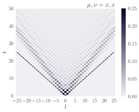
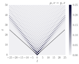
We consider the function in Eq. (19) for the discrete-time quantum walk in one-dimension and coin-angle for varying distance between the initial operators. Figure 2 shows the numerical results for at various time slices. We can identify the velocity of the wavefront as . In the present case, the OTOC function is “shell-like”. That is, inside the timelike region, in the long-time limit, , indicating no scrambling of operator , the vanishing of the OTOC in the long-time limit suggests that expansion of in terms of Pauli strings does not contain many pauli matrices “in the middle” of the strings. The feature common to Integrable quantum systems [69].
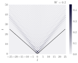
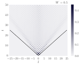
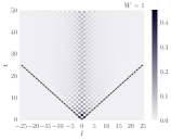
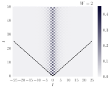
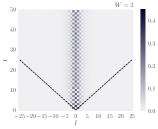
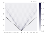
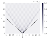
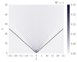
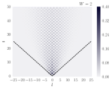

The disorder (both spatial and temporal) in a system causes a slowdown in information propagation (see Fig. 3). In particular, the spatial disorder results in Anderson localization which should be distinguished from MBL phase. The later is known as a non-interacting phenomenon. As the disorder strength increase, the shape of the light cone changes from ballistic to confine up to localization length for time showing no information propagation beyond localization length. As shown in Fig. 3, the spatial disorder leads to more rapid localization compared to temporal disorder as we increase disorder strength.
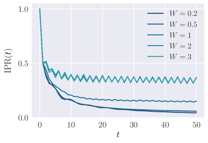
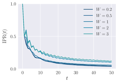
To characterize the localization, we consider inverse participation ratio (IPR) defined as [70]
| (20) |
where is probability of walker being at position and time . The IPR quantifies the number of basis states that effectively contribute to the system’s time evolution. Figure 4 shows the IPR calculated in presence of spatial and temporal disorder for varying disorder strength . In presence of disorder, the IPR saturates to a finite value which increase with disorder strength. The saturation value is larger in case of spatial compare to temporal showing that localization is strong in presence of spatial disorder.
V.2 K-complexity
Considering the formulation of K-complexity presented in Sec. III for discrete-time evolution, we can show that the discrete-time quantum walk exhibit linear growth. We will consider the initial operator to be of the form . At any time , the operator is given by
| (21) |
where the evolution operator . We will show that the set of operators form a orthogonal basis i.e. . First, we note that operators forms a orthogonal basis in position Hilbert space . Next, consider the operator
where and to unclutter notation and we used . More generally, the evolution of operator contains the linear combination of terms that are orthonormal to each other. In what follow, it will prove important to represent the operators as
| (24) |
where the blue dot represent the presence of term and multiple presence of blue dot represents the linear combination of these terms in operator expansion. The inner product between operators and corresponds depends on the expansion term corresponding to where dot color matches. The inner product between the operators in Eq. (24) is zero i.e. the operators are orthonormal to each other since there are no common blue dots. At , the operators given by
| (25) |
which shows and . In general, it follows that . If we define a matrix such that , it be such that it’s odd off-diagonal terms are zero. We now prove that even off-diagonal terms are equal to each other. To show this consider,
as required. In summary, we can write
| (26) |
Therefore, the krylov basis vector given by
As the dispersion in discrete-time quantum walk grows linearly, the amplitude , and therefore, . It follows that , hence the K-complexity given by
| (27) |
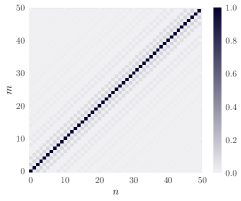
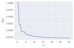
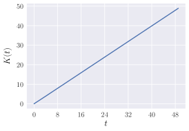
In Fig. 5, the numerical analysis is presented for K-complexity of the discrete-time quantum walk. The norm of operator saturates at a constant value close to showing that at late-time, the operators are approximately orthogonal to each-other. Therefore, the K-complexity obeys a linear growth.
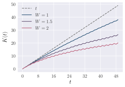

As we seen in Sec. V.1, the introduction of disorder leads to slowdown in information propagation. The K-complexity shows the similar localized behavior as OTOC in which it deviates from linear growth to suppress power law with . In this case, the amplitude goes to zero for large due to localization at . Therefore, the expansion coefficient is non-zero for small which results in suppressed growth in complexity. In Fig. 6, the K-complexity is calculated under temporal and spatial disorder in discrete-time quantum walk for increasing disorder strength . As with the OTOC, the suppression in K-complexity growth is smaller in temporal case compared to spatial as result of strong localization (or AL) in the later case.
VI Conclusion
In summary, the discrete-time quantum walks are quantum model which can be used to simulate a large number of phenomenon from quantum many-body physics as well as for construction of quantum algorithms. There experimental implementation on wide number of platform makes them suitable to study theoretical ideas. In this article, we studied information scrambling in discrete-time quantum walk using the out-of-time correlators and K-complexity as probe. The OTOC features the “shell-like” behavior, in which, at long-time limit, it goes to zero indicating no scrambling of the operator. The introduction of disorder (spatial or temporal) results in slowdown of information scrambling where the shape of light-cone confines up to localization length. The K-complexity shows a linear growth which ties to the fact that the operator at any time is approximately orthonormal to all operators at previous times. The disorder suppresses the K-complexity growth resulting its behavior of sub-linear. While the spatial disorder results in strong localization, the temporal disorder results in weak localization which is apparent from the behavior of both OTOC as well as K-complexity.
We would like to understand the effect of boundary conditions. In this work, we focused discrete-time quantum walk in infinite-dimensional 1D lattice, but from experimental point of view, it may be interesting to see the late-time behavior of these quantities . In ref. [71], the information scrambling was studied on Clifford quantum cellular automata (QCA). These systems shown to break ergodicity, i.e., they exhibit quantum scarring. It was further shown that such a system could exhibit classical dynamics in some semi-classical limit. While the discrete-time quantum walks are not the same as QCA, but they can be regarded as the dynamics of the one-particle sector of a QCA [72]. Therefore, it be interesting if the connection between the two results can be made more direct. In this direction, one should note that Clifford QCAs model studied in ref. [71] also exhibits linear growth in K-complexity. It follows from the evolution of operator under Clifford QCAs in which a string of pauli operators maps to another. Since the pauli operator form a orthonormal basis, each evolution step generate a new basis element resulting in linear growth. While for infinite-dimensional case, this growth will persist forever due infinite dimensional Hilbert space, in case of finite-dimensional lattice, the growth will stop as the operator get backs to its initial state. Therefore, the linear growth in K-complexity follows by a sudden decay to zero followed by repetitive behavior which is refinance of recurrence dynamics.
In this work, we formulated the K-complexity for the system with discrete-time evolution. Therefore, it opens up a way to consider more interesting many-body systems with discrete-time evolution. One such example could be random unitary circuits (RUCs) [73], which has been an active area of research for the past several years. RUCs have shed light on longstanding questions about thermalization and chaos and on the underlying universal dynamics of quantum information and entanglement [74]. While several works have explored the dynamics of OTOC in a number of variants of RUCs [75, 76], the study of K-complexity can further help understand post-scrambling-time behavior.
From the point of view of discrete-time quantum walks, which are the basis of many quantum algorithms, the study of information scrambling could provide the basis for designing algorithms that can efficiently explore the Hilbert spaces. In this context, the K-complexity which describe delocalization of operator in Hilbert space may be useful. Overall, the study of scrambling in both discrete-time quantum walks as well as in more generic systems with discrete-time evolution paves toward new physics in quantum many-body physics.
Acknowledgement: We wish to thank Aranya Bhattacharya for various useful discussions and comments about this and related works.
VII References
References
- Xu and Swingle [2024] S. Xu and B. Swingle, PRX Quantum 5, 010201 (2024).
- Lewis-Swan et al. [2019] R. J. Lewis-Swan, A. Safavi-Naini, A. M. Kaufman, and A. M. Rey, Nature Reviews Physics 1, 627 (2019).
- Deutsch [1991] J. M. Deutsch, Phys. Rev. A 43, 2046 (1991).
- Rigol et al. [2008] M. Rigol, V. Dunjko, and M. Olshanii, Nature 452, 854 (2008).
- Srednicki [1994] M. Srednicki, Phys. Rev. E 50, 888 (1994).
- Maldacena et al. [2016] J. Maldacena, S. H. Shenker, and D. Stanford, JHEP 08, 106 (2016), arXiv:1503.01409 [hep-th] .
- Yasuhiro Sekino and L. Susskind [2008] Yasuhiro Sekino and L. Susskind, Journal of High Energy Physics 2008, 065 (2008).
- Lashkari et al. [2013] N. Lashkari, D. Stanford, M. Hastings, T. Osborne, and P. Hayden, Journal of High Energy Physics 2013, 22 (2013).
- Shenker and Stanford [2014] S. H. Shenker and D. Stanford, JHEP 03, 067 (2014), arXiv:1306.0622 [hep-th] .
- Sahu et al. [2019] S. Sahu, S. Xu, and B. Swingle, Phys. Rev. Lett. 123, 165902 (2019).
- Swingle and Chowdhury [2017] B. Swingle and D. Chowdhury, Phys. Rev. B 95, 060201 (2017).
- McClean et al. [2018] J. R. McClean, S. Boixo, V. N. Smelyanskiy, R. Babbush, and H. Neven, Nature Communications 9, 4812 (2018).
- Haferkamp et al. [2023] J. Haferkamp, F. Montealegre-Mora, M. Heinrich, J. Eisert, D. Gross, and I. Roth, Communications in Mathematical Physics 397, 995 (2023).
- Shen et al. [2020] H. Shen, P. Zhang, Y.-Z. You, and H. Zhai, Phys. Rev. Lett. 124, 200504 (2020).
- Wu et al. [2021] Y. Wu, P. Zhang, and H. Zhai, Phys. Rev. Res. 3, L032057 (2021).
- Garcia et al. [2022] R. J. Garcia, K. Bu, and A. Jaffe, JHEP 03, 027 (2022), arXiv:2112.01440 [quant-ph] .
- Swingle [2018] B. Swingle, Nature Physics 14, 988 (2018).
- Rozenbaum et al. [2017] E. B. Rozenbaum, S. Ganeshan, and V. Galitski, Phys. Rev. Lett. 118, 086801 (2017).
- Parker et al. [2019] D. E. Parker, X. Cao, A. Avdoshkin, T. Scaffidi, and E. Altman, Phys. Rev. X 9, 041017 (2019).
- Barbón et al. [2019] J. L. F. Barbón, E. Rabinovici, R. Shir, and R. Sinha, JHEP 10, 264 (2019), arXiv:1907.05393 [hep-th] .
- Rabinovici et al. [2021] E. Rabinovici, A. Sánchez-Garrido, R. Shir, and J. Sonner, Journal of High Energy Physics 2021, 62 (2021).
- Rabinovici et al. [2022a] E. Rabinovici, A. Sánchez-Garrido, R. Shir, and J. Sonner, JHEP 07, 151 (2022a), arXiv:2207.07701 [hep-th] .
- Rabinovici et al. [2022b] E. Rabinovici, A. Sánchez-Garrido, R. Shir, and J. Sonner, JHEP 03, 211 (2022b), arXiv:2112.12128 [hep-th] .
- Bhattacharya et al. [2024] A. Bhattacharya, P. P. Nath, and H. Sahu, Phys. Rev. D 109, 066010 (2024).
- Jian et al. [2021] S.-K. Jian, B. Swingle, and Z.-Y. Xian, JHEP 03, 014 (2021), arXiv:2008.12274 [hep-th] .
- Bhattacharjee et al. [2023a] B. Bhattacharjee, P. Nandy, and T. Pathak, JHEP 08, 099 (2023a), arXiv:2210.02474 [hep-th] .
- He et al. [2022] S. He, P. H. C. Lau, Z.-Y. Xian, and L. Zhao, JHEP 12, 070 (2022), arXiv:2209.14936 [hep-th] .
- Caputa and Datta [2021] P. Caputa and S. Datta, JHEP 12, 188 (2021), [Erratum: JHEP 09, 113 (2022)], arXiv:2110.10519 [hep-th] .
- Khetrapal [2023] S. Khetrapal, JHEP 03, 176 (2023), arXiv:2210.15860 [hep-th] .
- Kundu et al. [2023] A. Kundu, V. Malvimat, and R. Sinha, JHEP 09, 011 (2023), arXiv:2303.03426 [hep-th] .
- Camargo et al. [2023] H. A. Camargo, V. Jahnke, K.-Y. Kim, and M. Nishida, JHEP 05, 226 (2023), arXiv:2212.14702 [hep-th] .
- Avdoshkin et al. [2022] A. Avdoshkin, A. Dymarsky, and M. Smolkin, (2022), arXiv:2212.14429 [hep-th] .
- Erdmenger et al. [2023] J. Erdmenger, S.-K. Jian, and Z.-Y. Xian, JHEP 08, 176 (2023), arXiv:2303.12151 [hep-th] .
- Trigueros and Lin [2022] F. B. Trigueros and C.-J. Lin, SciPost Phys. 13, 037 (2022), arXiv:2112.04722 [cond-mat.dis-nn] .
- Bento et al. [2023] P. H. S. Bento, A. del Campo, and L. C. Céleri, (2023), arXiv:2312.05321 [quant-ph] .
- Bhattacharya et al. [2022] A. Bhattacharya, P. Nandy, P. P. Nath, and H. Sahu, JHEP 12, 081 (2022), arXiv:2207.05347 [quant-ph] .
- Bhattacharjee et al. [2023b] B. Bhattacharjee, X. Cao, P. Nandy, and T. Pathak, JHEP 03, 054 (2023b), arXiv:2212.06180 [quant-ph] .
- Bhattacharya et al. [2023] A. Bhattacharya, P. Nandy, P. P. Nath, and H. Sahu, JHEP 12, 066 (2023), arXiv:2303.04175 [quant-ph] .
- Liu et al. [2023] C. Liu, H. Tang, and H. Zhai, Phys. Rev. Res. 5, 033085 (2023), arXiv:2207.13603 [cond-mat.str-el] .
- Bhattacharjee et al. [2024] B. Bhattacharjee, P. Nandy, and T. Pathak, JHEP 01, 094 (2024), arXiv:2311.00753 [quant-ph] .
- Venegas-Andraca [2012] S. E. Venegas-Andraca, Quantum Information Processing 11, 1015 (2012).
- Ambainis [2003] A. Ambainis, International Journal of Quantum Information 01, 507 (2003), publisher: World Scientific Publishing Co.
- Oka et al. [2005] T. Oka, N. Konno, R. Arita, and H. Aoki, Physical Review Letters 94, 100602 (2005).
- Barkhofen et al. [2018] S. Barkhofen, L. Lorz, T. Nitsche, C. Silberhorn, and H. Schomerus, Phys. Rev. Lett. 121, 260501 (2018).
- Xie et al. [2020] D. Xie, T.-S. Deng, T. Xiao, W. Gou, T. Chen, W. Yi, and B. Yan, Phys. Rev. Lett. 124, 050502 (2020).
- Manouchehri and Wang [2014] K. Manouchehri and J. Wang, Physical Implementation of Quantum Walks (Springer, Berlin, Heidelberg, 2014).
- Karski et al. [2009] M. Karski, L. Förster, J.-M. Choi, A. Steffen, W. Alt, D. Meschede, and A. Widera, Science 325, 174 (2009).
- Broome et al. [2013] M. A. Broome, A. Fedrizzi, S. Rahimi-Keshari, J. Dove, S. Aaronson, T. C. Ralph, and A. G. White, Science 339, 794 (2013).
- Wu et al. [2019] J. Wu, W.-W. Zhang, and B. C. Sanders, Frontiers of Physics 14, 61301 (2019).
- Swingle et al. [2016] B. Swingle, G. Bentsen, M. Schleier-Smith, and P. Hayden, Phys. Rev. A 94, 040302 (2016).
- Mi et al. [2021] X. Mi, P. Roushan, C. Quintana, S. Mandrà, et al., Science 374, 1479 (2021).
- Zhao et al. [2022] S. K. Zhao et al., Phys. Rev. Lett. 129, 160602 (2022).
- Gärttner et al. [2017] M. Gärttner, J. G. Bohnet, A. Safavi-Naini, M. L. Wall, J. J. Bollinger, and A. M. Rey, Nature Physics 13, 781 (2017).
- Braumüller et al. [2022] J. Braumüller et al., Nature Physics 18, 172 (2022).
- Landsman et al. [2019] K. A. Landsman, C. Figgatt, T. Schuster, N. M. Linke, B. Yoshida, N. Y. Yao, and C. Monroe, Nature 567, 61 (2019).
- Xu and Swingle [2020] S. Xu and B. Swingle, Nature Physics 16, 199 (2020).
- Xu and Swingle [2019] S. Xu and B. Swingle, Phys. Rev. X 9, 031048 (2019).
- Khemani et al. [2018] V. Khemani, D. A. Huse, and A. Nahum, Phys. Rev. B 98, 144304 (2018).
- Chandrashekar [2013a] C. M. Chandrashekar, Scientific Reports 3, 2829 (2013a).
- Chandrashekar [2013b] C. M. Chandrashekar, (2013b), arXiv:1212.5984 [quant-ph] .
- Chandrashekar et al. [2008] C. M. Chandrashekar, R. Srikanth, and R. Laflamme, Phys. Rev. A 77, 032326 (2008).
- Chandrashekar [2011] C. M. Chandrashekar, Phys. Rev. A 83, 022320 (2011).
- Toikka [2020] L. A. Toikka, Phys. Rev. B 101, 064202 (2020).
- Vakulchyk et al. [2017] I. Vakulchyk, M. V. Fistul, P. Qin, and S. Flach, Phys. Rev. B 96, 144204 (2017).
- Malishava et al. [2020] M. Malishava, I. Vakulchyk, M. Fistul, and S. Flach, Phys. Rev. B 101, 144201 (2020).
- Zeng and Yong [2017] M. Zeng and E. H. Yong, Scientific Reports 7, 12024 (2017).
- Kumar et al. [2018] N. P. Kumar, S. Banerjee, and C. M. Chandrashekar, Scientific Reports 8, 8801 (2018).
- Vieira et al. [2013] R. Vieira, E. P. M. Amorim, and G. Rigolin, Phys. Rev. Lett. 111, 180503 (2013).
- Lin and Motrunich [2018] C.-J. Lin and O. I. Motrunich, Phys. Rev. B 97, 144304 (2018).
- Evers and Mirlin [2008] F. Evers and A. D. Mirlin, Rev. Mod. Phys. 80, 1355 (2008).
- Kent et al. [2023] B. Kent, S. Racz, and S. Shashi, Phys. Rev. B 107, 144306 (2023).
- Farrelly [2020] T. Farrelly, Quantum 4, 368 (2020).
- Fisher et al. [2023] M. P. Fisher, V. Khemani, A. Nahum, and S. Vijay, Annual Review of Condensed Matter Physics 14, 335 (2023).
- Nahum et al. [2017] A. Nahum, J. Ruhman, S. Vijay, and J. Haah, Phys. Rev. X 7, 031016 (2017).
- Nahum et al. [2018] A. Nahum, S. Vijay, and J. Haah, Phys. Rev. X 8, 021014 (2018).
- Weinstein et al. [2023] Z. Weinstein, S. P. Kelly, J. Marino, and E. Altman, Phys. Rev. Lett. 131, 220404 (2023).