Stochastic ordering of series and parallel systems’ lifetime in Archimedean copula under random shock
Abstract
In this manuscript, we studied the stochastic ordering behavior of series as well as parallel systems’ lifetimes comprising dependent and heterogeneous components, experiencing random shocks, and exhibiting distinct dependency structures. We establish certain conditions for the lifetime of individual components, the dependency among components defined by Archimedean copulas, and the impact of random shocks on the overall system lifetime to reach the conclusion. We consider components whose survival functions are either increasing log-concave or decreasing log-convex functions of the parameters involved and systems exhibit different dependency structures. These conditions make it possible to compare the lifetimes of two systems using the usual stochastic order framework. Additionally, we provide examples and graphical representations to elucidate our theoretical findings.
Keywords
Usual stochastic order; majorization; super-additive(Sub-additive) function; schur-convex(Schur-concave) function.
MSC Classification
Primary: 60E15.
Secondary: 90B25; 62G30.
1 Introduction
In theory of reliability, a -component system is termed as -out-of- system if it remains operational if at least of the total components are working. Denote the -th order statistic by , of the random variables which denotes the lifetime of a out-of- system. In the past few decades, some articles have studied the stochastic ordering of order statistics when the random variables represent the lifetimes of components, assuming that the component’s lifetimes are identically and independently distributed. For example, Proschan and Sethuraman (1976), Pledger and Proschan (1971), Bergmann (1991), Nelsen (2006), Kochar (2007), and Kochar (2012) have studied these systems and compared the lifetimes of different systems. However, the lifetimes of components in a system may or may not be independently and identically distributed. To deal with the dependency and heterogeneity among the lifetimes of components, the multivariate Archimedean copula plays a significant role in the stochastic ordering of order statistics and comparing the reliabilities of systems, for reference few articles are Balakrishnan and Zhao (2013), Li and Fang (2015), Balakrishnan et al. (2020), Erdely et al. (2014) and Zhang et al. (2019) for the relevant theory dealing with non-identical and dependent components. In practical scenarios, the components may exhibit dependencies, and different systems may exhibit different dependency structures among their components. Furthermore, various external random shocks in the components may affect the lifetimes of the system. Zhang et al. (2018) considered the case when the components are independently distributed and derived results for the stochastic ordering of the lifetimes of two fail-safe systems subject to random shock. Balakrishnan et al. (2018) derived some results regarding the largest claim amounts from two heterogeneous portfolios. However, the claims are assumed to be independent. The most recent article by Amini-Seresht et al. (2024) focuses on the stochastic ordering of the lifetimes of series and parallel systems under the assumption that components are dependent and non-identical, all the systems exhibit the same dependency structure, represented by the same Archimedean copula, under the presence of random shocks in the components. But, in general, different systems may exhibit different dependency structures among their components’ lifetime. So, It’s naturally interesting to explore the circumstance in which the components within the system undergo random shocks, and survive after the random shocks with certain probabilities, and different systems exhibit different dependency structures among the components’ lifetime. Das et al. (2022) studied the smallest insurance claim amounts from two portfolios using a very restricted model (exponentiated location-scale model) with several conditions imposed on the parameters and the generator. In this document, we’ll study the stochastic comparison of lifetimes between series systems as well as parallel systems. We consider that the dependency structures among the components’ lifetimes are represented by different Archimedean copulas with generators denoted by and (with pseudo-inverses , respectively). The components of the systems may experience random shocks, and their lifetimes follow distribution models with increasing log-concave or decreasing log-convex survival functions in parameters, which are very general models in statistical analyses.
This manuscript is structured as follows: Section two presents several established concepts and theorems in the form of lemmas that are useful for the remaining sections. Section three discusses some results for the stochastic ordering of series and parallel systems in the presence of random shock when the composition function is super-additive. Section four delves into the case when the composition function is sub-additive. We conclude the manuscript in section five.
2 Preliminaries
Let’s begin by revisiting certain concepts and important lemmas that are fundamental to the subsequent main findings. We employ the following notations where bold font represents vectors in .
Let be a random vector with dependent and non-identically distributed random variables and , where represents the CDF (cumulative distribution function) of and denotes the parameter of the distribution of , for . Suppose that the survival function of , for , is denoted by . Moreover, consider be independent of ’s, , for . Here, are employed to signify whether the system’s components, having random lifetimes , have survived or failed after experiencing the random shock. Specifically, if , then component survives after experiencing a random shock; else, if , the component fails to survive after experiencing a random shock, for . Therefore, the random variables represent the lifetimes of the systems’ components, subject to random shock effect and we denote , for . Hence, is comprising two random variables: first one is with CDF , the second one is a Bernoulli random variable with mean . Following simple proof steps we find, the survival function of is , for each . Therefore,
Definition 2.1.
(Def 2.4 Li and Fang (2015)) Let be a non-increasing and continuous function such that and , let be the pseudo-inverse of , the function defined as
is called Archimedean copula and is known as Archimedean generator for if for and is non-increasing and convex. Archimedean copula gives us joint CDF in terms of the generator when the marginal CDFs are given. Similarly, Archimedean survival copula is defined. It relates the survival function of joint distribution to the survival functions of marginal distributions.
Note:
If is a random vector with marginal CDFs and the Archimedean copula generator , then the CDF of -th order statistics is,
Now if is the generator of the Archimedean survival copula, Then the survival function of the -st order statistics is,
Definition 2.2.
Consider two random variables X and Y with CDFs F and G respectively and survival functions and , respectively. Then Y is called greater than X in the sense of usual stochastic order ( i.e., ) if for all .
Now we state some results in the form of lemmas that are useful in the remaining part of the manuscript.
Lemma 2.1.
(Marshall et al. (2011), Theorem 5.A.2) Consider the function h, which is increasing, and concave (convex), then for .
Lemma 2.2.
(Marshall et al. (2011), Theorem 3.A.4) If a function is continuously differentiable and permutation-symmetric, then it is Schur-convex (or Schur-concave) on if and only if is symmetric on and satisfies, for all ,
Lemma 2.3.
(Marshall et al. (2011), Def A.1., ch 3) Consider the function then, if and only if is a Schur-convex (Schur-concave) function on .
Lemma 2.4.
(Marshall et al. (2011), Theorem 3.A.8) Consider the function then, if and only if is decreasing (increasing) and Schur-convex function on .
Lemma 2.5.
(Marshall et al. (2011), Theorem A.8) Consider the function then, for , if and only if is both increasing (decreasing) and Schur-convex (Schur-concave) function on .
Lemma 2.6.
(Li and Fang (2015), Lemma A.1) Let and be two -dimentional Archimedean copulas with generators and (with pseudo-inverses and ) respectively, if is a super-additive (sub-additive) function, then for all . That is,
3 Main results for the super-additive case
We state the first result which compares the reliability of two parallel systems when components’ survival functions are increasing and log-concave in parameters of the distributions, components are subject to random shocks, and the composition function is a super-additive.
Theorem 3.1.
Consider two dependent and heterogenous random vectors and , where , and are independent of ’s and ’s for . Further, consider that and possess Archimedean copulas generated by and respectively and . Then if
, is super-additive and
or is increasing in .
be increasing and log-concave function of the parameter .
Proof.
The CDF of the random variable is
Using super-additivity of we get that
| (1) |
Now we will prove that
| (2) |
For this, we will consider the function defined as
.
We now show that it is a Schur convex function and decreases in each argument.
Here,
this shows that is decreasing in when other arguments are kept constant. Now consider,
Without loss of generality suppose that . Note that and since . Now using , increasing property of and log-concave property of in , we get,
Remark 3.1.
Theorem 3.1. provides insight into the fact that when the survival functions of the components are increasing and log-concave, systems possess different dependency structures, and components are experiencing random shocks, we can establish a stochastic ordering of the parallel system’s lifetimes. It is important to note that there are many copula generators and survival functions satisfying conditions in theorem 3.1. A few examples are provided below.
(i) Regarding conditions (i) and (ii) of Theorem 3.1, consider and be two generators of Clayton copula defined by and inverses with parameters and respectively, then for we have,
this implies is a convex function and hence a super-additive function for and for are increasing functions of . For another example, consider two AMH copulas with parameters and , then both the condition (i) and (ii) are satisfied [see Zhang et al. (2019) Remark 3.5 for reference].
(ii) Regarding condition (iii) on the survival functions of the components, we can find many survival functions that are increasing and log-concave simultaneously in parameters. For example, exponential distribution with mean and survival function , log-logistic distribution with (increasing and log-concave w.r.t scale parameter ), parallel systems when components are from proportional reversed hazard model, etc.
Remark 3.2.
The above Theorem 3.1. generalizes Theorem 3.4 of Amini-Seresht et al. (2024) when the dependency structure among the components of two parallel systems and are described by two different Archimedean copulas with generators and respectively and is a super-additive function. Because if, in particular, , then is a super-additive function and then above Theorem 3.1. becomes the Theorem 3.4 of Amini-Seresht et al. (2024).
(i) Since the super-majorization in the above Theorem 3.1. is more general condition than majorization condition in Theorem 3.4 of Amini-Seresht et al. (2024), therefore Theorem 3.1. is true in more general parallel systems than that of Theorem 3.4 of Amini-Seresht et al. (2024).
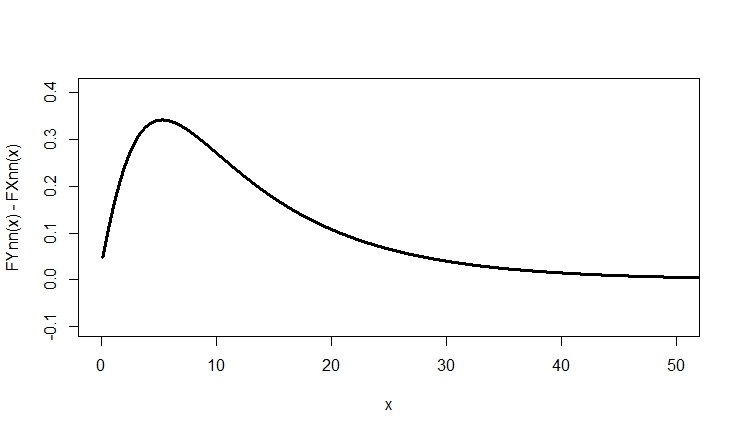
Example 3.1.
Consider random vectors and where and where, , and
. Then it is easy to observe that is increasing in and is a concave function of .
Now consider the multivariate AMH copulas generated by and so that then we get, is an increasing function of and . Some straightforward manipulations gives which is an increasing function for and , implies it is a convex function with . Hence is a super-additive function, see Remark 3.5 of Zhang et al. (2019) for reference.
The graph of is shown below for and to illustrate it is a non-negative function of .
The theorem presented below is regarding the usual stochastic ordering of two parallel systems when the survival functions of the components are decreasing and the log-convex function of the parameter , components may experience random shock and parallel systems may show different dependency structures.
Theorem 3.2.
Consider two dependent and heterogenous random vectors and , where , and are independent of ’s and ’s for . Further, consider that and possess Archimedean copulas generated by and respectively and . Then if
, is super-additive and
or is decreasing in .
be decreasing and log-convex function of the parameter .
Proof.
Proceeding in the similar manner as the proof of we have,
We will shows that is a Schur-concave function. Now consider,
.
.
Remark 3.3.
Theorem 3.2. provides insight into the fact that when the survival functions of the components are decreasing and log-convex, systems possess different dependency structures and components are experiencing random shocks, we can establish a stochastic ordering of the parallel systems’ lifetimes. Some examples of Archimedean generators satisfying the conditions of are as follows.
(i) consider the Gumbel copula with Archimedean generators defined by where for . Then and which is a super-additive function if . Further, is a non-increasing function of for .
(ii) Consider Gumbel-barnett copulas with Archimedean generators where for . Then and . Differentiating two times we have,
Therefore is a convex function, hence a super-additive function for . Further, is decreasing function for , where .
(iii) It’s worth mentioning that survival functions of the components is decreasing and log-convex function in parameters in Theorem 3.2., is very common in practice and such examples of survival functions can be found easily. Some examples of such survival functions are Weibull distribution (in scale parameter ) with survival functions , exponential distribution with mean , components following proportional hazard model, additive hazard model etc.
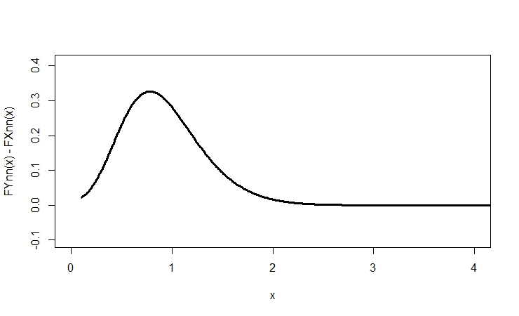
Example 3.2.
Condsider random vectors and where and (Weibull distribution with shape parameter ) where, , and . Then observe that is decreasing in and is a convex function of .
Now consider the multivariate Gumbel-Barnett copulas generated by where for in the . Then all the conditions of are satisfied for .
The graph of is shown below for and to illustrate it is a non-negative function of .
The theorem presented below is regarding the usual stochastic ordering of lifetimes of two series systems when components’ survival functions are increasing and log-concave in parameters for , systems show different dependency structures and components are subject to random shocks.
Theorem 3.3.
Consider two dependent and heterogenous random vectors and , where , and are independent of ’s and ’s for . Further, consider that and possess Archimedean copulas generated by and respectively and . Then if
, is super-additive and , ,
or is increasing function.
be increasing and log-concave function of the parameter .
Proof.
The survival function of is .
Using super-additivity of we get that
| (3) |
Now we will prove that
| (4) |
For this, we will consider the function defined as
We now show that it is a Schur-concave function.
Here,
| (5) |
Now consider,
Without loss of generality suppose that . Note that and since . Now using , increasing property of , non-positivity of and log-cocave property of w.r.t . We get,
Remark 3.4.
The above Theorem 3.3. Generalizes Theorem 3.8 of (Amini-Seresht et al., 2024) when the dependency structure among the components of two series systems are described by two different Archimedean copulas with generators and respectively.
Remark 3.5.
Theorem 3.3. provides insight into the fact that when the survival function of the components is increasing and log-concave, systems possess different dependency structures and components are experiencing random shocks, we can establish a stochastic ordering of the lifetimes of series systems. There are many Archimedean copula generators and survival functions satisfying conditions in Theorem 3.3.
(i) Consider Gumbel copulas with the generator defined by and for . Then, It follows that
are non-negative functions for and . Further, is super-additive for .
(ii) Consider the Clayton copulas having generator and . Then simple manipulation gives,
is super-additive for , are satisfied. For further details, one may refer to page 147 of Amini-Seresht et al. (2024). On the other hand, examples of increasing and log-concave survival functions are given in .
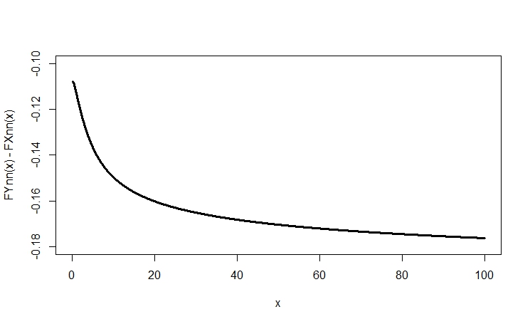
Example 3.3.
Consider the random vectors and where and where, , and
. The survival function of log-logistic distribution, is increasing in and is a concave function of .
Now consider the Gumbel copulas with the generators defined by and for of . Then these generators satisfy the required conditions of Theorem 3.3 for as shown in .
The graph of is shown below for and to illustrate it is a non-positive function of .
The theorem presented below is regarding the usual stochastic ordering of two series system when the survival functions of the components are decreasing and a log-convex function of the parameter , components may experience random shock and parallel systems may show different dependency structures.
Theorem 3.4.
Consider two dependent and heterogenous random vectors and , where , and are independent of ’s and ’s for . Further, consider that and possess Archimedean copulas generated by and respectively and . Then if
, is super-additive and , , .
or is decreasing function.
be decreasing and log-convex function of the parameter .
Proof.
Proceeding similarly to the proof of we have,
| (6) |
This shows that is decreasing in each argument when other arguments are kept constant.
Now consider,
Without loss of generality suppose that . Note that and since . Now using , decreasing property of , non-positivity of and log-convex property of w.r.t . We get,
Remark 3.6.
Theorem 3.4. sheds light on the fact that when the survival functions of the components are decreasing and log-convex in parameters, systems possess different dependency structures and components are experiencing random shocks, we can establish a stochastic ordering of the lifetimes of series systems.
Remark 3.7.
Following examples of Archimedean generators are provided in support of the Theorem 3.4.
(i) Regarding conditions of theorem 3.4., consider (Remark 1. of Fariba Ghanbari et al. (2023)) and be two generators of Gumbel-Hougaard copula given by generators and , then for and , we have, is super-additive. Now consider the inverse of the generator for and . Simple manipulation shows that,
for and . Therefore the function is decreasing for and .
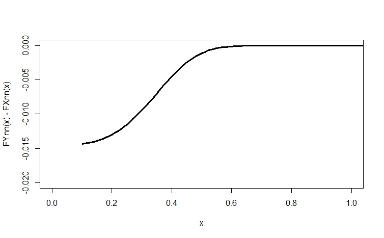
Example 3.4.
Condsider random vectors and where and (Weibull distribution with shape parameter ) where, , and . Then is decreasing in and is a convex function of .
Now consider the Gumbel-Hougaard copula in Remark 3.7(i). Then these generators satisfy the required conditions of Theorem 3.4 for as shown in .
The graph of is shown below for and to illustrate it is a non-positive function of .
4 Main results for the sub-additive case
In Section 3 we have generalized Theorem 3.4. and Theorem 3.8. of Amini-Seresht et al. (2024) when different dependency structures are shown by the systems and described by Archimedean copulas with generators and . However, we have considered the case when the composition is super-additive. But in practice may or may not be a super-additive function. This Section 4 will shed light on the usual stochastic ordering of first and highest-order statistics when the composition function is a sub-additive and the survival functions of components are either an increasing log-concave or a decreasing log-convex in parameters.
Now we state a result that compares the reliability of two parallel systems when components’ survival functions are increasing and log-concave in parameters of the distributions and components may experience random shocks.
Theorem 4.1.
Consider two dependent and heterogenous random vectors and , where and and are independent of ’s and ’s for . Further, consider that and possess Archimedean copulas generated by and respectively and . Then if
, is sub-additive and .
or is increasing in .
be increasing and log-concave function of the parameter .
Proof.
The CDF of is
Using sub-additivity of we get that
| (7) |
Now we will show that
| (8) |
For this, we will consider the function defined as
.
After that, following similar steps to the proof of Theorem 3.1, we get is a decreasing Schur-convex function. Now using Lemma 2.4, . Which is the inequality (8). Combining (7) and (8) we get .
∎
Remark 4.1.
The above Theorem 4.1. generalizes Theorem 3.4 of Amini-Seresht et al. (2024) when the dependency structure among the components of two parallel systems and are described by two different Archimedean copulas with generators and respectively and is a sub-additive function. Because if, in particular, , then is a sub-additive function and then above Theorem 4.1. becomes the Theorem 3.4 of Amini-Seresht et al. (2024).
(i) Since the super-majorization in the above Theorem 4.1. is a more general condition than majorization condition in Theorem 3.4 of Amini-Seresht et al. (2024), therefore Theorem 4.1. is true in more general parallel systems than parallel systems considered in Theorem 3.4 of Amini-Seresht et al. (2024).
(ii) It is very crucial to see that in , Clayton copula generators gives,
this implies is a concave function and hence a sub-additive function for and for are increasing functions of . Similarly for the AMH copula family if then becomes a concave function, therefore, a sub-additive function.
The theorem presented below is regarding the usual stochastic ordering of two parallel systems when the survival functions of the components are decreasing and a log-convex function of the parameter , components may experience random shock and parallel systems may show different dependency structures.
Theorem 4.2.
Consider two dependent and heterogenous random vectors and , where and and are independent of ’s and ’s for . Further, consider that and possess Archimedean copulas generated by and respectively and . Then if
, is sub-additive and
or is decreasing in .
be decreasing and log-convex function of the parameter .
Proof.
Remark 4.2.
Consider the Gumbel copula in , we have,
Now if then becomes a concave function hence a sub-additive function. For other conditions see . Similarly, if we consider the Gumbel-barnett copula in we have,
. Now if then becomes a concave function hence a sub-additive function.
The theorem presented below is regarding the usual stochastic ordering of two series system’s lifetimes when components survival functions are increasing and a log-concave in parameters for , systems show different dependency structures and components are subject to random shock.
Theorem 4.3.
Consider two dependent and heterogenous random vectors and , where , and are independent of ’s and ’s for . Further, consider that and possess Archimedean copulas generated by and respectively and . Then if
, is sub-additive and , ,
or is increasing function.
be increasing and log-concave function of the parameter .
Proof.
The survival function of the random variable is .
Remark 4.3.
Consider Gumbel copula in , where generators are defined by and for . Then we have,
are non-negative functions for , and . Further, is sub-additive for . Similarly, for Clayton copula generators in ,
is sub-additive for and .
The theorem presented below is regarding the usual stochastic ordering of series systems when the survival functions of the components are decreasing and the log-convex function of the parameter , components may experience random shock and parallel systems may show different dependency structures.
Theorem 4.4.
Consider two dependent and heterogenous random vectors and , where , and are independent of ’s and ’s for . Further, consider that and possess Archimedean copulas generated by and respectively and . Then if
, is sub-additive and , , .
or is decreasing function.
be decreasing and log-convex function of the parameter .
Proof.
Proceeding in the similar manner to the proof of we have,
| (13) |
Now we will show that
| (14) |
For this, we will consider the function defined as
After that, following similar steps as Theorem 3.4., we get is decreasing and Schur-convex function. Using Lemma 2.4, . Which is the inequality (14). Combining (13) and (14) we get . ∎
Remark 4.4.
Consider Gumbel-Hougaard copula in , given by the generators,
and , then we have,
is a non-positive function for , , and . Therefore is a concave function, hence a sub-additive function for . Now consider the inverse of the generator for and . A simple manipulation shows that,
for and . Therefore the function is decreasing for and .
5 Conclusion
In this article, we studied usual stochastic ordering of series and parallel systems when the components survival functions are either an increasing log-concave or a decreasing log-convex function in parameters, and components may experience random shocks. We also consider that the systems exhibit different dependency structures. An interesting observation is that, if (with inverse ) and (with inverse ) are Archimedean generators for two random vectors of concerning series (or parallel) systems with lifetimes and respectively, then the usual stochastic order reversed to when the composition is changed from super-additive to sub-additive. Further investigation could focus on scenarios where the systems possess distinct random shock structures.
Funding information
Sarikul Islam is being financially supported through a research grant allocated by the Ministry of Human Resource Development (MHRD) of the Government of India.
Competing interests
There are no competing interests to declare that arose during the preparation of this article.
References
- Amini-Seresht et al. [2024] Ebrahim Amini-Seresht, Ebrahim Nasiroleslami, and Narayanaswamy Balakrishnan. Comparison of extreme order statistics from two sets of heterogeneous dependent random variables under random shocks. Metrika, 87(2):133–153, 2024.
- Balakrishnan and Zhao [2013] Narayanaswamy Balakrishnan and Peng Zhao. Ordering properties of order statistics from heterogeneous populations: a review with an emphasis on some recent developments. Probability in the Engineering and Informational Sciences, 27(4):403–443, 2013.
- Balakrishnan et al. [2018] Narayanaswamy Balakrishnan, Yiying Zhang, and Peng Zhao. Ordering the largest claim amounts and ranges from two sets of heterogeneous portfolios. Scandinavian Actuarial Journal, 2018(1):23–41, 2018.
- Balakrishnan et al. [2020] Narayanaswamy Balakrishnan, Ghobad Barmalzan, and Abedin Haidari. Exponentiated models preserve stochastic orderings of parallel and series systems. Communications in Statistics-Theory and Methods, 49(7):1592–1602, 2020.
- Bergmann [1991] Reinhard Bergmann. Stochastic orders and their application to a unified approach to various concepts of dependence and association. Lecture Notes-Monograph Series, pages 48–73, 1991.
- Das et al. [2022] Sangita Das, Suchandan Kayal, and N Balakrishnan. Ordering results for smallest claim amounts from two portfolios of risks with dependent heterogeneous exponentiated location-scale claims. Probability in the Engineering and Informational Sciences, 36(4):1116–1137, 2022.
- Erdely et al. [2014] Arturo Erdely, Jose M Gonzalez-Barrios, and Mara M Hernandez-Cedillo. Frank condition for multivariate archimedean copulas. Fuzzy Sets and Systems, 240:131–136, 2014.
- Fariba Ghanbari et al. [2023] . Fariba Ghanbari, Ghobad Barmalzan, and Reza Hashemi. Stochastic comparisons of series and parallel systems with dependent log-logistic components. Communications in Statistics-Theory and Methods, 52(12):4259–4282, 2023.
- Kochar [2007] Subhash Kochar. Stochastic orders by m. shaked and jg shantikumar, 2007.
- Kochar [2012] Subhash Kochar. Stochastic comparisons of order statistics and spacings: a review. International Scholarly Research Notices, 2012, 2012.
- Li and Fang [2015] Xiaohu Li and Rui Fang. Ordering properties of order statistics from random variables of archimedean copulas with applications. Journal of Multivariate Analysis, 133:304–320, 2015.
- Marshall et al. [2011] Albert W Marshall, Ingram Olkin, Barry C Arnold, Albert W Marshall, Ingram Olkin, and Barry C Arnold. Preservation and generation of majorization. Inequalities: Theory of Majorization and Its Applications, pages 165–202, 2011.
- Nelsen [2006] Roger B Nelsen. Archimedean copulas. An introduction to copulas, pages 109–155, 2006.
- Pledger and Proschan [1971] Gordon Pledger and Frank Proschan. Comparisons of order statistics and of spacings from heterogeneous distributions. In Optimizing methods in statistics, pages 89–113. Elsevier, 1971.
- Proschan and Sethuraman [1976] F Proschan and J Sethuraman. Stochastic comparisons of order statistics from heterogeneous populations, with applications in reliability. Journal of Multivariate Analysis, 6(4):608–616, 1976. ISSN 0047-259X. doi: https://doi.org/10.1016/0047-259X(76)90008-7. URL https://www.sciencedirect.com/science/article/pii/0047259X76900087.
- Zhang et al. [2018] Yiying Zhang, Ebrahim Amini-Seresht, and Peng Zhao. On fail-safe systems under random shocks. Applied Stochastic Models in Business and Industry, 35, 05 2018. doi: 10.1002/asmb.2349.
- Zhang et al. [2019] Yiying Zhang, Xiong Cai, Peng Zhao, and Hairu Wang. Stochastic comparisons of parallel and series systems with heterogeneous resilience-scaled components. Statistics, 53(1):126–147, 2019.