sO¿\SplitArgument1—mP\IfBooleanTF#1\PPauto#3\PPfixed#2#3\NewDocumentCommand\PPautomm(\IfNoValueTF#2#1#1 — #2)\NewDocumentCommand\PPfixedmmm#1(\IfNoValueTF#3#2#2#1—#3#1)\NewDocumentCommand\PCsO¿\SplitArgument1—mcov\IfBooleanTF#1\PCauto#3\PCfixed#2#3\NewDocumentCommand\PCautomm(\IfNoValueTF#2#1#1 — #2)\NewDocumentCommand\PCfixedmmm#1(\IfNoValueTF#3#2#2#1—#3#1) \stackMath \newsiamremarkremarkRemark \newsiamremarkhypothesisHypothesis \newsiamthmclaimClaim \headersProbabilistic Budget-Constrained Binary OptimizationAhmed Attia
Probabilistic Approach to Black-Box Binary Optimization with Budget Constraints: Application to Sensor Placement††thanks: Submitted to the editors . \funding This material is based upon work supported by the U.S. Department of Energy, Office of Science, Office of Advanced Scientific Computing Research (ASCR), ASCR Applied Mathematics Base Program, and Scientific Discovery through Advanced Computing (SciDAC) Program through the FASTMath Institute under contract number DE-AC02-06CH11357 at Argonne National Laboratory.
Abstract
We present a fully probabilistic approach for solving binary optimization problems with black-box objective functions and with budget constraints. In the proposed probabilistic approach, the optimization variable is viewed as a random variable and is associated with a parametric probability distribution. The original binary optimization problem is then replaced with an optimization over the expected value of the original objective, which is then optimized over the probability distribution parameters. The resulting optimal parameter (optimal policy) is used to sample the binary space to produce estimates of the optimal solution(s) of the original binary optimization problem. The probability distribution is chosen from the family of Bernoulli models given the binary nature of the optimization variable. The optimization constraints generally restrict the feasibility region. This effect can be achieved by modeling the random variable with a conditional distribution given satisfiability of the constraints. Thus, in this work we develop conditional Bernoulli distributions to model the binary random variable conditioned by the total number of nonzero entries, that is, the budget constraint. This approach (a) is generally applicable to binary optimization problems with nonstochastic black-box objective functions and budget constraints; (b) accounts for budget constraints by employing conditional probabilities that sample only the feasible region and thus considerably reduces the computational cost compared with employing soft constraints; and (c) does not employ soft constraints and thus does not require tuning of a regularization parameter, for example to promote sparsity, which is challenging in sensor placement optimization problems. The proposed approach is verified numerically by using an idealized bilinear binary optimization problem and is validated by using a sensor placement experiment in a parameter identification setup.
keywords:
Binary and Combinatorial Optimization, Black-box Optimization, Probabilistic Optimization, Neuro-dynamic Programming, Reinforcement Learning and Constrained Policy Optimization, Optimal Experimental Design, Optimal Sensor Placement.90C27, 60C05, 62K05, 35R30, 35Q93, 65C60, 93E35.
1 Introduction
This paper describes a fully probabilistic approach for solving budget-constrained binary (or categorical) optimization problems of the form
| (1) |
where the objective function is a black-box real-valued deterministic function. We use maximization in (1); however, the approaches and analyses presented in this work apply equally to minimization problems. This will be highlighted in the discussion as needed. This is an NP-hard combinatorial optimization problem that arises, with various complexities of the objective , in abundant applications including machine learning and computer vision [22, 36, 51, 28, 52, 55]; natural and social sciences and social network analysis [33, 23, 59]; healthcare and drug discovery [29, 57]; and a wide range of economics and engineering applications [56, 44]. Solving such binary optimization problems in large-scale applications by brute force is computationally infeasible because the solution space grows exponentially with the dimension of . Specifically, for , the number of possible realization of is .
Of special interest is the problem of optimal resource allocation and optimal sensor placement in large- to extreme-scale data assimilation and inverse problems [18, 27, 42, 17, 16]. This problem is usually formulated as a model-constrained optimal experimental design (OED) [49, 30, 45, 54, 2, 6, 4, 1, 9, 10]. The OED objective function is a utility function that often quantifies the information gain from an experiment, and the optimization problem is constrained by a simulation model and sparsity constraint (e.g., budget constraints) on to avoid simply dense designs. This is usually achieved by using an penalty/regularization term that is inherently nonsmooth. Thus, smooth approximations of the penalty term are employed, and the binary sensor placement problem is replaced with an approximate continuous relaxation that is then solved approximately following a gradient-based approach [10, 3, 10, 32, 37, 58].
A stochastic learning (probabilistic) approach for solving unconstrained binary optimization problems without the need for relaxation was introduced in [11] and extended to robust (e.g., max-min) optimization problems in [12]. This approach views the target optimization variable as a random variable, associates a parametric probability distribution (policy) to that variable, and replaces the binary optimization problem with an optimization problem over the parameters (probabilities) of the probability distribution. Specifically, the objective is replaced with an expectation surface , and the resulting optimization problem is solved by following a stochastic gradient approach. Thus the probabilistic approach has similarities with neuro-dynamic programming, reinforcement learning, and policy optimization [21, 19]. The optimal set (the set of optimal solutions) of the stochastic optimization problem includes the optimal solutions of the original optimization problem, and the optimal policy enables exploration (sampling) of the optimal set, for example in the case of nonunique optima.
The probabilistic approach is ideal for binary optimization with black-box objectives because it only requires evaluations of the objective at sampled realizations of the binary variable . The budget and sparsity promoting constraints can be embedded in the optimization objective function as penalty terms [11, 47]. This approach, however, introduces the need for expensive tuning of the penalty parameter, which is generally a challenging task especially when robust optimization is required because tuning the penalty parameter by using traditional methods such as the L-curve can fail due to the bilevel nature of the optimization problem. Heuristic approaches have been employed to enforce hard constraints [50, 48, 47] including budget constraints. These heuristics, however, are problem specific and still explore the full probability space and are thus computationally intensive and are not always guaranteed to yield a feasible solution.
This paper presents a fully probabilistic approach for binary optimization problems with black-box objective functions and with budget/cost constraints. The main idea is that constraints in an optimization problem define a restriction on the domain by defining a feasible region (set of all points satisfying the constraints) among which an optimal solution is sought. This corresponds to conditioning in probability distributions. Specifically, one can define the probability distribution of a random variable given that (conditioned on) a function of that variable (or another variable) satisfies a set of constraints, for example, equality or inequality constraints. Our approach employs a conditional distribution that defines the probability of conditioned by the budget constraints and thus explores only the feasible region. Developing conditional distributions for hard constraints is generally a nontrivial task, and of course various conditional models need to be modeled for different types of constraints. In this work we focus on budget constraints that can be extended to many types of binary constraints. Moreover, the work provides a rigorous foundation for handling other hard constraints in binary optimization with black-box objectives.
Contributions
The main contributions of this work are summarized as follows.
-
1.
We present an extensive treatment of a class of conditional Bernoulli models suitable for modeling budget constraints in binary optimization. The existing theory and computational methods for this class of probability models are very sparse and are limited to degenerate probabilities. Specifically, we considerably extend the Poisson binomial and the conditional Bernoulli models to properly handle degenerate probabilities. Moreover, we develop analytical forms of the derivatives needed for the proposed optimization approach, discuss moments (first- and second-order moments), and develop bounds on derivatives that are at the heart of the convergence analysis of the proposed approach. In addition to the crucial role these derivatives play in the proposed approach, they are suitable in general for model fitting, for example, maximum likelihood fitting.
-
2.
We propose a fully probabilistic approach that employs the developed probability models, and we provide a complete algorithmic statement for solving binary optimization problems with black-box objectives and budget constraints. This approach can be used as a plug-and-play tool for solving a wide range of sensor placement optimization and decision-making problems where the objective can be treated as a black box.
-
3.
We discuss the convergence of the proposed approach and analyze its performance, strength, and limitations.
- 4.
-
5.
We carry out an extensive numerical analysis for the proposed approach using an idealized bilinear binary optimization problem, and an OED optimal sensor placement experiment to verify the quality of the proposed approach.
The rest of the paper is organized as follows. Section 2 provides the mathematical background and overviews the probabilistic approach to unconstrained binary optimization. Section 3 provides a detailed discussion of the probability models required for the proposed probabilistic optimization approach, which is presented in Section 4. Numerical results are described in Section 5, and conclusions are summarized in Section 6.
2 Background: Unconstrained Binary Optimization via Stochastic Learning
The probabilistic optimization approach [11] aims to solve the unconstrained binary optimization problem
| (2) |
by regarding as a random variable following a multivariate Bernoulli distribution with independent but not identically distributed Bernoulli trials associated with success probabilities . The joint probability mass function (PMF) is thus given by
| (3) |
with an expectation given by
| (4) |
where all possible realizations of are labeled as . Note that the indexing scheme only associates each possible with a unique integer index . The main idea is that the expectation (4) constructs a smooth surface—as a function of success probabilities—that connects all possible realizations of the binary random variable . Thus, the probabilistic approach to unconstrained binary optimization [11] replaces the original problem (2) with the following stochastic optimization problem,
| (5) |
which can be solved by following a stochastic gradient approach. Specifically, the gradient of (5) can be approximated efficiently by using Monte Carlo samples from the corresponding policy, that is, the multivariate Bernoulli distribution with parameter ,
| (6) |
where is a sample drawn from the Bernoulli distribution with success probabilities . The gradient of the log-probability model (written in terms of its elements) is given by where is the th normal vector (versor) in . Thus, the gradient and its stochastic approximation (6) only require the values of the objective at sampled realizations of . The cost of sampling and evaluation of the gradient of the log probability is negligible, and the cost of the process is exclusively dependent on the cost of evaluating . For example, when involves evaluations of simulation models such as partial differential equations, the cost can be significantly reduced by employing surrogate and reduced-order models; see, for example, [31].
As discussed in [11], the stochastic approximation of the gradient is an unbiased estimator. Its variance, however, can deteriorate the performance of stochastic gradient-ascent (in the case of maximization) or gradient-descent (in the case of minimization) optimization procedures. Thus, variance reduction methods are generally employed to reduce the variability of the stochastic gradient while maintaining its unbiasedness. This can be achieved by using antithetic variates for sampling, importance sampling, optimal baselines, or a combination thereof.
Modeling budget constraints
To account for hard (e.g., budget) constraints, one can employ soft constraints where a penalty term is appended to the objective to enforce a given constraint on [11, 12]. This approach, however, requires choosing a penalty/regularization parameter large enough to enforce the constraint but also small enough to avoid domination of the objective function value over the constraint. While approaches such as the L-curve [39, 41] can be employed to tune the penalty parameter, this approach is generally problematic (e.g., the robust formulation) and is computationally expensive. Moreover, despite the reduction of the feasible region due to the constraints, with employing soft constraints the whole domain of is still sampled, leading to considerable waste of computational efforts and even inaccuracies in the solution procedure since the result is not guaranteed to satisfy the budget constraint.
An alternative approach is to employ heuristics to enforce the budget constraint. For example, Ryu et al. [50] enforce the budget constraint by a simple heuristic that orders the success probabilities in decreasing order and samples each entry , by comparing the corresponding success probability with a uniform random sample until the budget constraint is fulfilled. While this is a simple approach, it has no guarantees and can fail in fulfilling the budget constraint. The main reason is that such heuristics change the sampling process, which means the samples generated are not distributed according to the multivariate Bernoulli distribution being optimized.
Proper modeling of the hard constraints in general requires restricting the feasible region by modeling the random variable by a conditional probability distribution given satisfiability of the hard constraints. Specifically, in order to employ (5) for solving (1), the random variable needs to be modeled by a conditional probability distribution . Developing such a conditional distribution is a nontrivial task and is dependent on the type of the constraints. In this work we focus on budget constraints suitable for decision-making, sensor placement, and OED, as defined by (1).
3 Probability Models
In this section we develop the probability models that will model the budget constraints in the probabilistic optimization approach proposed in Section 4. This section is self-contained and presents a comprehensive analysis of the probability distributions of interest. The reader interested only in the proposed optimization approach can skip to Section 4 and get back to referenced models and identies in this section as needed.
Section 3 provides new developments and major extensions to combinatoric relations and probability models those are essential for the probabilistic approach proposed in Section 4. Specifically, we develop and analyze the following probability models:
| (7) |
where is a collection of binary random variables (Bernoulli trials) with success probabilities , where .
The first probability model in (7) is the multivariate Bernoulli model (3), which assumes the trials are independent but not identically distributed. The second probability model describes the probability of achieving a total number of successes (number of entries equal to ) in the trials. If the success probabilities are equal, this could be modeled by a binomial distribution. Since the success probabilities are not necessarily identical, however, this distribution is described by the Poisson binomial (PB) model [25]. The third probability model describes the probability of an instance of the binary variable , that is, a collection of the binary trials, conditioned by their sum. This distribution can be defined by extending the conditional Bernoulli (CB) model [25].
The unconditional multivariate Bernoulli model is fully developed and well understood; see, for example, [11, Appendix A]. Thus, in the rest of this section we focus on developing the PB and CB models, respectively. First, in Section 3.1 we develop a set of preliminary relations and computational tools essential for formulating and analyzing both models. The PB model is then described in Section 3.2, and the CB model is presented in Section 3.3. For clarity of notation, and since all probability models discussed in this work are parameterized by the success probabilities , we drop the dependence on from all distributions and state it explicitly only when needed to avoid confusion. Additionally, for clarity of the discussion, the proofs of theorems and lemmas introduced in Section 3 are provided in Appendix A.
3.1 Preliminary relations
A combinatoric function that is elementary to formulating and evaluating the joint probabilities of both PB and CB models (7) is the R-function, defined as
| (8) |
where is the set of indices associated with all Bernoulli trials. Thus, the R-function evaluates the sum of products of weights corresponding to all possible combinations of different choices of Bernoulli trials . As an example, let with non-degenerate success probabilities . By defining the set of indices and the weights and by considering the case where in (8), then , , , . Of course, as the dimensionality increases, the R-function cannot be practically evaluated by enumeration. Efficient evaluation of the R-function is addressed in Section 3.1.2.
Lemma 3.1 describes the derivative of the weights vector (8), which will be essential for developing derivatives of the probability models with respect to their parameters.
Lemma 3.1.
Let be a Bernoulli random vector with parameter , and consider the vector of weights with entries defined by (8). Then
| (9) |
where is the identity matrix and is a diagonal matrix with on its main diagonal.
Proof 3.2.
See Appendix A.
3.1.1 Inclusion probability
The inclusion probability (also known as the coverage probability) is the probability that a unit is selected when a sample of size is selected at random from a given population of size . Because this is the probability of a single unit inclusion, it is generally referred to as the first-order inclusion probability and is generally given a symbol . Generally speaking, the th-order inclusion probability is the probability that the tuple/set of unique units is included in a sample of size drawn without replacement from a population of size [53]. For the general case of weighted sampling, and assuming each element of the population is associated with a probability of being selected in a sample of size , the th-order inclusion probability (see, e.g., [25, 53]) is given by
| (10) |
where for two sets , the set difference is obtained by excluding elements of set from set . For example, the first- and second-order inclusion probabilities, respectively, are given by
| (11) |
The first-order inclusion probability can be interpreted in the case of Bernoulli trials as follows. Assume we are sampling a multivariate Bernoulli random variable such that only entries are allowed to be equal to . In this case, the probability of the th entry to be equal to in a random draw of is . Note that for a fixed sample size , the first- and second-order inclusion probabilities (11) satisfy the following relations (see, e.g., [53] ):
| (12) |
with derivative information described by Lemma 3.3.
Lemma 3.3.
First- and second-order inclusion probabilities (11) satisfy the following identities:
| (13a) | ||||
| (13b) | ||||
| (13c) | ||||
| (13d) | ||||
| where is the Kronecker delta function, . | ||||
Proof 3.4.
See Appendix A.
Corollary 3.5 follows immediately from Lemma 3.3 by definition of logarithm derivative and by using Lemma 3.1.
Corollary 3.5.
3.1.2 Efficient evaluation of the R-function
As mentioned earlier, evaluating the R-function by enumerating all possible combinations, that is, by using (8), is computationally challenging and can be infeasible for large cardinality. The value of the R-function, however, can be calculated efficiently by using one of the following recurrence relations [25, 35, 40, 38]. For any nonempty set ,
| (15a) | ||||
| (15b) | ||||
| (15c) | ||||
The initial condition of the R-function is given by
| (15d) |
which can also be obtained by setting in (15a). As stated in [25, Section 2], the first recurrence (15a) requires a total of additions and multiplications to compute . The second relation (15a), on the other hand, requires additions and multiplications. Thus, both methods cost . The first method, however, can be numerically unstable given that the values of grow exponentially.
The recurrence relation (15b) is used to tabulate the values of recursively where the th row (starting with index ) corresponds to the values of for subsets with cardinality . A tabulation procedure that employs this relation was presented in [25, Table 3], in which cell in the table is generated by , where the first row is filled with by using the fact that , as stated earlier. The tabulation procedure is summarized in (Figure 1), and we will build on it for evaluating derivatives of the R-function; see Section 3.1.3. Unlike (15a), each iteration of the tabulation procedure resulting from (15b) requires only maintaining values of , which considerably reduces memory requirements.
3.1.3 Derivatives of the R-function
The probability distributions discussed later in this work rely on the R-function, and thus we need to develop a method to efficiently evaluate the gradient of this function. Since the recurrence (15a) is generally numerically unstable for large cardinality (we have tested that already), we focus on the tabulation procedure based on (15b).
To apply (15b), the tabulation procedure (see, e.g., Figure 1) calculates each cell by using the relation , which means one can calculate the gradient of each cell recursively to the tabulation procedure similar to the principle of automatic differentiation. Specifically, , where we used the fact that . Thus, to evaluate the gradient of the cells in the th row of the table recursively, we need to keep track of both the values and the derivatives of the cells on the previous row of the table. Specifically, the gradient is computed recursively by the following tabulation procedure (along with the tabulation of R-function evaluation). The first row is set to for all values of , and each cell is given by the relation . To formalize this approach, we use the same example given by Figure 1 to describe the tabulation procedure for gradient evaluation in Figure 2. Note that the tabulation procedure provides the first-order derivative of the R-function with respect to the Bernoulli weights (8). The gradient with respect to the Bernoulli probabilities can be obtained by applying the chain rule and by employing Lemma 3.1.
In addition to the method described above for gradient tabulation, we can define derivatives of the R-function using inclusion probabilities as summarized by Lemma 3.6.
Lemma 3.6.
Proof 3.7.
See Appendix A.
Corollary 3.8 follows immediately from Lemma 3.6 by the definition of logarithm derivative and by using Lemma 3.1.
Corollary 3.8.
The significance of Lemma 3.6 and Corollary 3.8 is that they provide closed forms of the gradient of the R-function and also provide second-order derivative information. Despite being data parallel—components of the gradient and the Hessian can be computed completely in parallel—each entry of the gradient requires evaluating the R-function for a different set and thus requires constructing a table for each entry to calculate first-order probabilities.
3.2 Poisson binomial distribution
In this section we discuss the PB model, which models the sum of independent Bernoulli trials with different success probabilities [25]. In other words, the PB distribution models the probability of the norm of a multivariate Bernoulli random variable. Let , where is a multivariate Bernoulli random variable with non-degenerate success probabilities . Then follows a PB distribution with joint PMF given by
| (18) |
The R-function (Section 3.1) will be used to evaluate the PMF and its derivatives. Specifically, the gradient of the PMF of the PB distribution (18) with respect to the distribution parameters is described by the following Lemma 3.9.
Lemma 3.9.
Let be the sum of a multivariate Bernoulli random variable with success probabilities and weights calculated elementwise. Then
| (19a) | ||||
| (19b) | ||||
Proof 3.10.
See Appendix A.
Corollary 3.11 follows immediately from Lemma 3.9 and Lemma 3.6. Note that while (20) simplifies the derivative formulation, it is more computationally expensive to apply than (19) since it requires constructing an independent table for each of the inclusion probabilities. Nevertheless, these formulae will make it easier to carry out convergence analysis because we know the bounds and behavior of the weights and the inclusion probabilities as well as the probabilities .
Corollary 3.11.
Let be the sum of a multivariate Bernoulli random variable with success probabilities and weights calculated elementwise. Then
| (20a) | ||||
| (20b) | ||||
where is a vector consisting of first-order inclusion probabilities (11) and all operations on the vectors and are entrywise.
3.2.1 The degenerate case
So far, we have assumed the parameter of the PB model, that is, the success probabilities are non-degenerate . This is mainly due to the utilization of the R-function in evaluating the PMF and the associated derivatives. An important question is what happens at the bounds of the probability domain, that is, when any of the success probabilities is equal to either or . Here we extend the PB model (18) to include the case of degenerate probabilities. It is sufficient to consider the case where only one entry of is degenerate/binary, since the following arguments can be applied recursively. Lemma 3.12 describes the properties of the PB model at the boundary of the domain of the th success probability .
Lemma 3.12.
Proof 3.13.
See Appendix A.
The significance of Lemma 3.12 is that it shows that the PMF of the PB model and its derivative with respect to the parameters (probabilities of success) are both smooth. Moreover, it provides a rigorous definition the PMF and its derivative for the degenerate case where the weights employed in the R-function and in (18) are not defined, that is, when . Theorem 3.14 describes a generalization of the PB model where the success probabilities are allowed to be degenerate. The proof is eliminated because it follows immediately from (18) and (21).
Theorem 3.14.
| Let be a multivariate Bernoulli random variable with success probabilities . Let be the sum of entries of , that is, the total number of successes in Bernoulli trials, and let | |||
| (22a) | |||
| Then the PMF of the PB model over the closed interval is given by | |||
| (22b) | |||
| and the gradient of the PMF with respect to the distribution parameters is | |||
| (22c) | |||
| where is the th normal vector in . | |||
Proof 3.15.
See Appendix A.
3.3 The conditional Bernoulli distribution
The CB model [24] models the distribution of a random vector composed of Bernoulli trials with success probabilities conditioned by the total number of successes, that is, . Given the non-degenerate probabilities of success , the PMF of the CB model (often denoted by ) is given by
| (23) |
where the Bernoulli weights and the R-function are as described in Section 3.1. The gradient of the CB model PMF (23) is summarized by Lemma 3.16.
Lemma 3.16.
Let be a multivariate Bernoulli random variable with success probabilities , and let . Then
| (24a) | ||||
| (24b) | ||||
where the vector of weights is defined by (8) and is described by Section 3.1.3.
Proof 3.17.
See Appendix A.
While (24a) enables efficient evaluation of the first-order derivatives of the CB model PMF with respect to its parameters, we can employ first- and second-order inclusion probabilities to formulate equivalent formulae for both first- and second-order derivatives. This is summarized by Lemma 3.18.
Lemma 3.18.
Proof 3.19.
See Appendix A.
3.3.1 Moments of the CB model
Here we analyze the conditional expectation and conditional variance-covariance under the CB model. Specifically, Lemma 3.20 summarizes important identities for both first- and second-order moments under the CB model.
Lemma 3.20.
| (26a) | ||||
| (26b) | ||||
| (26c) | ||||
| (26d) | ||||
| (26e) | ||||
| where the total variance of the gradient , in the last equation, is defined as the sum of variances of its entries. | ||||
Proof 3.21.
See Appendix A.
3.3.2 The degenerate case
Similar to the treatment of the degenerate case of a degenerate PB model presented in Section 3.3.2, Lemma 3.22 describes the properties of a degenerate CB model.
Lemma 3.22.
The CB model (23) satisfies the following identities.
| (27a) | ||||
| (27b) | ||||
| (27c) | ||||
| (27d) | ||||
| (27e) | ||||
| (27f) | ||||
| (27g) | ||||
| (27h) | ||||
Proof 3.23.
See Appendix A.
Lemma 3.22 enables us to handle degenerate/binary success probabilities in a CB model as follows. First, the Bernoulli sum is reduced by the number of probabilities (entries in ) equal to . Second, the dimension is reduced by the number of binary entries by removing the entries of and corresponding to probabilities in . To formalize this procedure, we conclude this section with Theorem 3.24, which summarizes the most important identities of the CB model given the discussion presented above. The proof of the theorem is omitted because it follows immediately from the definition of the CB model’s PMF for non-degenerate probabilities (23) and Lemma 3.22.
Theorem 3.24.
| Let be a multivariate Bernoulli random variable with success probabilities . Let be the sum of the entries of , that is, the total number of successes in Bernoulli trials, and let | |||
| (28a) | |||
| Then the PMF of the CB model over the closed interval is given by | |||
| (28b) | |||
| where and the gradient of the PMF with respect to the distribution parameters is where where is the th normal vector in and the partial derivatives for are given by | |||
| (28c) | |||
| such that both the PMF and its derivative are continuous for . | |||
Proof 3.25.
See Appendix A.
3.4 Generalized conditional Bernoulli model
Here we introduce a formal generalization to the CB model (28) where the scalar is replaced with a set of admissible values. Specifically, Lemma 3.26 describes a generalized CB (GCB) model that describes the probability distribution of a multivariate Bernoulli random variable conditioned by multiple possibilities of the sum .
Lemma 3.26.
Proof 3.27.
See Appendix A.
The significance of Lemma 3.26 is that it enables employing the PB model and the CB model to evaluate probabilities, moments, and gradients under the GCB model.
3.5 Sampling
Here we provide the machinery for generating samples from the probability distributions discussed in Section 3.
3.5.1 Sampling the PB distribution
Sampling a PB distribution (22b) amounts to weighted random sampling with replacement from the set , where the weights (probabilities) are defined by the PB PMF (22b) for each value in this set. Hence, sampling a PB distribution is straightforward. In the reset of this section we focus on sampling the CB and the GCB models described in Section 3.5.2 and Section 3.5.2, respectively.
3.5.2 Sampling the CB distribution
One can sample exactly from a CB model [25, 38] or use alternative methods such as Markov chain Monte Carlo; see, for example, [34]. Here, for completeness, we summarize an algorithm that samples the CB model exactly; see [34, Appendix A]. To sample a CB model (28b) with success probabilities and conditioned by the value of the sum , we follow two steps. First, we define a matrix-valued function with entries (with indices starting at ) given recursively by
| (30) |
Second, we utilize the following sequential decomposition of the CB model to generate a sample. Each entry of a CB random variable is sampled sequentially by calculating the corresponding probability conditioned by previous entries and by the distribution parameter, and by the sum . The inclusion probability of the th entry, that is, the probability of setting the entry to , is
| (31) | ||||
which formulates the probability in terms of the matrix-valued function (30). Thus, by using (30) and (31), we can sample realizations from a CB model sequentially. Note that the matrix defined by (30) is sparse and is fixed for fixed parameters . This procedure is summarized by Algorithm 1.
3.5.3 Sampling the GCB distribution
Generating a random sample of size from the generalized CB model (29a) is carried out in two steps. First, a set of realizations of the parameter is drawn with replacement from the set by using weighted random sampling with weights equal to the probabilities dictated by the PB distribution (18), that is, . Second, for each realization in the collected sample, use Algorithm 1 to draw a sample from the CB model with parameters .
4 Probabilistic Black-Box Binary Optimization
Here we describe a fully probabilistic approach for solving binary optimization problems with black-box objective functions and budget/cost constraint (1). We start in Section 4.1 by discussing in detail the case of budget equality constraints. We then describe in Section 4.2 a generalization that addresses the case of budget inclusion (e.g., inequality) constraint. For clarity, the proofs of theorems and lemmas introduced in Section 4 are provided in Appendix B.
4.1 Budget equality constraint
Here we focus on the optimization problems of the form
| (32) |
where is a real-valued black-box deterministic function. This formulation is especially important for resource allocation and sensor placement applications where the objective is to maximize an expensive utility function that involves black-box code simulations and nonsmooth objectives.
The probabilistic approach [11] views each as a Bernoulli trial and associates a probability with those trials. Since the binary variable must be confined to the subspace defined by the budget constraints, the trials are no longer uncorrelated, and we need to model the distribution of probabilistically by using a probability distribution model conditioned by the budget constraint. This is achievable in this case by employing the CB model presented in Section 3.3. Thus, we employ the CB model (28b) and replace the optimization problem (32) with the following stochastic optimization problem:
| (33a) | ||||
| whose gradient (derivative with respect to the distribution parameter ) is given by | ||||
| (33b) | ||||
where independence of from , linearity of the expectation, and the kernel trick () are used to obtain the last term. The set of optimal solutions of (32) is guaranteed to be a subset of the optimal set of (33a); see [11, Lemma 3.2]. In order to solve (33a) following a gradient-based approach, a stochastic approximation of the gradient (33b) is used in practice. The stochastic gradient is given by
| (34a) | |||
| (34b) | |||
where the PMF is given by (28b) and the gradient is given (elementwise) by (28c). To use the stochastic gradient (34) to approximately solve (33a), an algorithm takes a step of a predefined size (learning rate) in the direction of the gradient in the case of maximization or in the opposite direction in the case of minimization. We must, however, restrict the update to the domain of the optimization parameter/variable . Thus, we must use a projector to project the gradient onto . Here we use a scaling projection operator that works by reducing the magnitude of the gradient if the gradient-based update is outside the domain . The projection operator is given by
| (35) |
where in the definition of is added to define the projected gradient based on the update for both maximization and minimization, respectively. A stochastic steepest ascent step to solve (33a) is approximated by the stochastic approximation of the gradient (34) and is described as
| (36) |
where is the step size (learning rate) at the th iteration. The plus sign in (36) is replaced with a negative sign for minimization (steepest descent) problems.
Employing the projector (35) has the potential of simplifying the problem of tuning the learning rate (optimization step size). One can choose a fixed step size or follow a decreasing schedule to guarantee convergence. In fact, by using this projector, we were able to fix the learning rate in our numerical experiments as discussed in Section 5. Note, however, that other projection operators can be used, such as the truncation operator [43, Section 16.7] that was employed in [11]. However, our empirical studies indicated that (35) achieves a superior performance in this framework.
As discussed in [11], the stochastic gradient given by (34) is an unbiased estimator with variance that can be reduced by employing a baseline. Specifically, a baseline-based version of the gradient is given by
| (37) |
which is also unbiased, , with total variance (sum of elementwise variances) satisfying , with . Thus, we take the total variance as a quadratic expression in and minimize it over . Because , the quadratic is convex, and the min in is obtained by equating the derivative of the estimator variance to zero. We note that based on the values of the objective, we need to make sure the baseline is non-negative; otherwise, . Thus, the optimal baseline is , which is then approximated based on a sample collected from the CB model with parameter set by the current value of . By employing (26e), we have
| (38) |
which is independent from the sample collected to estimate the gradient. The value of , however, is estimated by using the collected sample as follows,
| (39) |
which yields the following optimal baseline estimate:
| (40) |
where only non-degenerate probabilities of success are employed in (40), , and the first-order inclusion probabilities are given by (11). If all success probabilities are degenerate, the baseline is set to since in this case and the variance of the baseline version of the stochastic gradient is no longer quadratic in .
4.2 Budget inclusion constraint
Here we focus on the optimization problems in the following more general form,
| (41) |
Similar to the case of equality constraint discussed in Section 4.1, we replace the optimization problem (41) with the following stochastic optimization problem:
| (42) |
with gradient
| (43) |
which is approximated by the following stochastic approximation:
| (44) |
with given by (29b) and given by (29a). Developing a version of the stochastic gradient (44) with minimum variance, following a baseline approach—subtracting a constant non-negative baseline from the objective value in the computation of the gradient—is achieved by defining the vector , whose total variance can be obtained by elementwise application of (29e). This results in the following baseline (minimum-variance) version of the stochastic gradient:
| (45a) | ||||
| (45b) | ||||
which, combined with a projection operator (35), is employed in a stochastic steepest ascent step to solve (42), as described by (36). In Section 4.4 we describe an algorithm that employs (33a) or (42) for solving (32), or (41), respectively.
4.3 Relation between binary and probabilistic formulations
Theorem 4.1 states the relation between the binary optimization problems and the corresponding probabilsitic counterparts discussed in Section 4.1 and Section 4.2.
Theorem 4.1.
Given the CB model (28b), the optimal solutions of the two problems (32) and (33a) are such that
| (46) |
and if the solution of (32) is unique, then , where is the unique optimal solution of (33a). Similarly, given the GCB model (29a), the optimal solutions of the two problems (41) and (42) are such that
| (47) |
and if the solution of (41) is unique, then , where is the unique optimal solution of (42).
Proof 4.2.
The proof follows immediately from [11, Lemma 3.2 and Proposition 3.1] by noting that we are restricting the support of the probability distribution only to the feasible region defined by the respective constraints.
The significance of Theorem 4.1 is that it shows that by solving the probabilistic optimization problem we obtain a set of parameters of the corresponding probability distributions that include the optimal set of the original binary optimization problem. Moreover, by sampling the underlying probability distribution (e.g,. CB or GCB), with the parameter set to the optimal solution of the probabilistic optimization problem, one obtains a set of binary realizations of with at least a near-optimal objective value as suggested in [11] and as shown in Section 5.
4.4 Algorithmic statement
Here we provide a complete algorithmic statement (Algorithm 3) that details the steps of the proposed probabilistic approach to binary optimization for solving (32) and (41).
Note that Algorithm 3 inherits the advantages of the original stochastic optimization algorithm [11, Algorithm 3.2]. Specifically, the value of is evaluated repeatedly at instances of binary variable , which are more likely/frequently revisited as the algorithm proceeds. Thus, redundancy in computation is prevented by keeping track of the sampled binary variables and the corresponding value of . This can be achieved by assigning a unique index or a hash value to each feasible value of . Algorithm 3 is conceptual, because the loop (Step 2) is not necessarily a finite processes. In practice, we can ensure that the loop is finite by setting a tolerance of the projected gradient and/or a maximum number of iterations.
4.5 Convergence analysis
Proving convergence of Algorithm 3 in expectation to the solution of the corresponding binary optimization problem requires developing bounds on the first- and second-order derivatives of the exact gradient and ensuring that the corresponding stochastic gradient approximation is an unbiased estimator and has bounded variance [11].
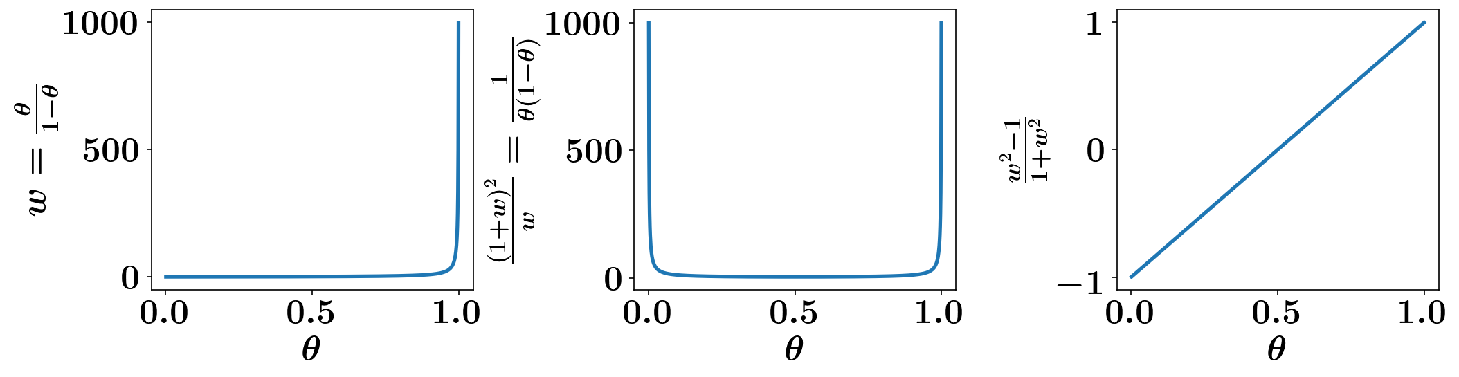
Evaluations of the CB model (28b), and thus the generalized version (29a), rely primarily on the weights (8) of the non-degenerate entries, which appear in several forms in the formulae of the first- and second-order derivatives of the PMF and its logarithm. For non-degenerate success probabilities , the weights satisfy the following upper bounds, with corresponding plots shown in Figure 3:
| (48) |
The bounds (48) are employed to develop the bounds on the derivatives of the CB model described by Theorem 4.3.
Theorem 4.3.
Proof 4.4.
See Appendix B.
The significance of Theorem 4.3 is that it enables developing bounds on the exact derivatives of the objective in (33a) as described in Theorem 4.5. Specifically, Theorem 4.5 shows that the exact gradient and the exact Hessian of are both bounded, which shows that the stochastic objective is Lipschitz smooth and guarantees convergence of steepest descent approach for solving (33a) to a local optimum solution.
Theorem 4.5.
Let , be modeled by the CB model (23), and let . Then the following bounds of the gradient of the stochastic objective in (33a) hold:
| (50a) | |||||
| (50b) | |||||
| (50c) | |||||
where , , and is the cardinality of the feasible domain. Moreover, if is in the degenerate case, that is, when follows (28b), then there is a finite constant such that
| (51) |
Proof 4.6.
See Appendix B.
From Theorem 4.5 it follows that similar bounds can be developed for the stochastic objective (42). This follows immediately from Lemma 3.26 by noting that for the GCB model (29a), the probabilities, derivatives, and first- and second-order moments are weighted linear combinations of the corresponding values of the CB model (28b). Note that the value of the upper bound in (51) itself is irrelevant here because only the existence of this finite constant guarantees convergence of a gradient-based optimization algorithm involving the exact gradient of the stochastic objective .
To guarantee convergence of the proposed Algorithm 3 we need to show that the stochastic estimate of the gradient is unbiased with bounded variance. This is shown by Theorem 4.7.
Theorem 4.7.
Proof 4.8.
See Appendix B.
Theorem 4.7 shows that the stochastic gradient employed in Algorithm 3 is an unbiased estimator and it satisfies Assumption (d) of [20, Assumptions 4.2], which guarantees convergence of the stochastic optimization algorithm, as discussed in [11]. Note that the convergence of the stochastic optimization procedure Algorithm 3, where baseline versions of the stochastic gradient are employed, is guaranteed by Theorem 4.7 and by the fact that for a finite positive constant , as was discussed in the derivation of the optimal baseline estimates; see, for example, the discussion in Section 4.1.
5 Numerical Experiments
We use a simple bilinear binary optimization problem in Section 5.1 to extensively validate the proposed approach. Then in Section 5.2, we further validate the probabilistic optimization approach by using an optimal sensor placement problem often utilized for experimental verification in the OED literature; see, for example, [46, 9, 10, 3, 5].
All numerical experiments in this work are carried out by using PyOED [26, 8] with the code to replicate all results available through PyOED’s examples and tutorials.
5.1 Numerical experiments using a bilinear binary optimization problem
In this section we employ the following objective function to formulate and solve probabilistic binary optimization problems with equality and inclusion/inequality constraints, in Section 5.1.1 and Section 5.1.2, respectively:
| (53) |
This function enables us to inspect global optimum (maximum or minimum) values and thus to study the performance of the proposed approach for various settings as discussed next. In all experiments here, we run Algorithm 3 with the maximum number of iterations set to , we set the the sample size of the stochastic gradient to , and we collect sample points from the policy generated at the last iteration of the optimization procedure to get an optimal design estimate. We compare the results with points sampled uniformly (by setting success probabilities to ) from the set of feasible observational designs.
We choose the learning rate and set the gradient tolerance pgtol to . The algorithm terminates if the maximum number of iterations is reached or if it has converged. Convergence is achieved if the magnitude of the projected gradient (35) is below the preset pgtol.
Solution by enumeration (brute force) is carried out for all feasible realizations of based on the defined budget constraint, and the corresponding value of is recorded for visualization when computationally feasible.
The initial success probabilities is set to ; that is, we set in Algorithm 3. Upon termination, the optimization algorithm returns samples from the underlying probability model (CB or GCB based on the type of the constraint) associated with the parameter at the final step. Then, it picks as the sampled design associated with the largest value of .
5.1.1 Results with equality budget constraint
First we run Algorithm 3 to solve the following optimization problem:
| (54) |
That is, we set the budget to , and we initially set the dimension to . The global maximum value of over the feasible region in this case is . Moreover, the cardinality of the feasible region, that is, the total number of feasible realizations of such that , is , which enables inspecting the objective value of all feasible realizations of .
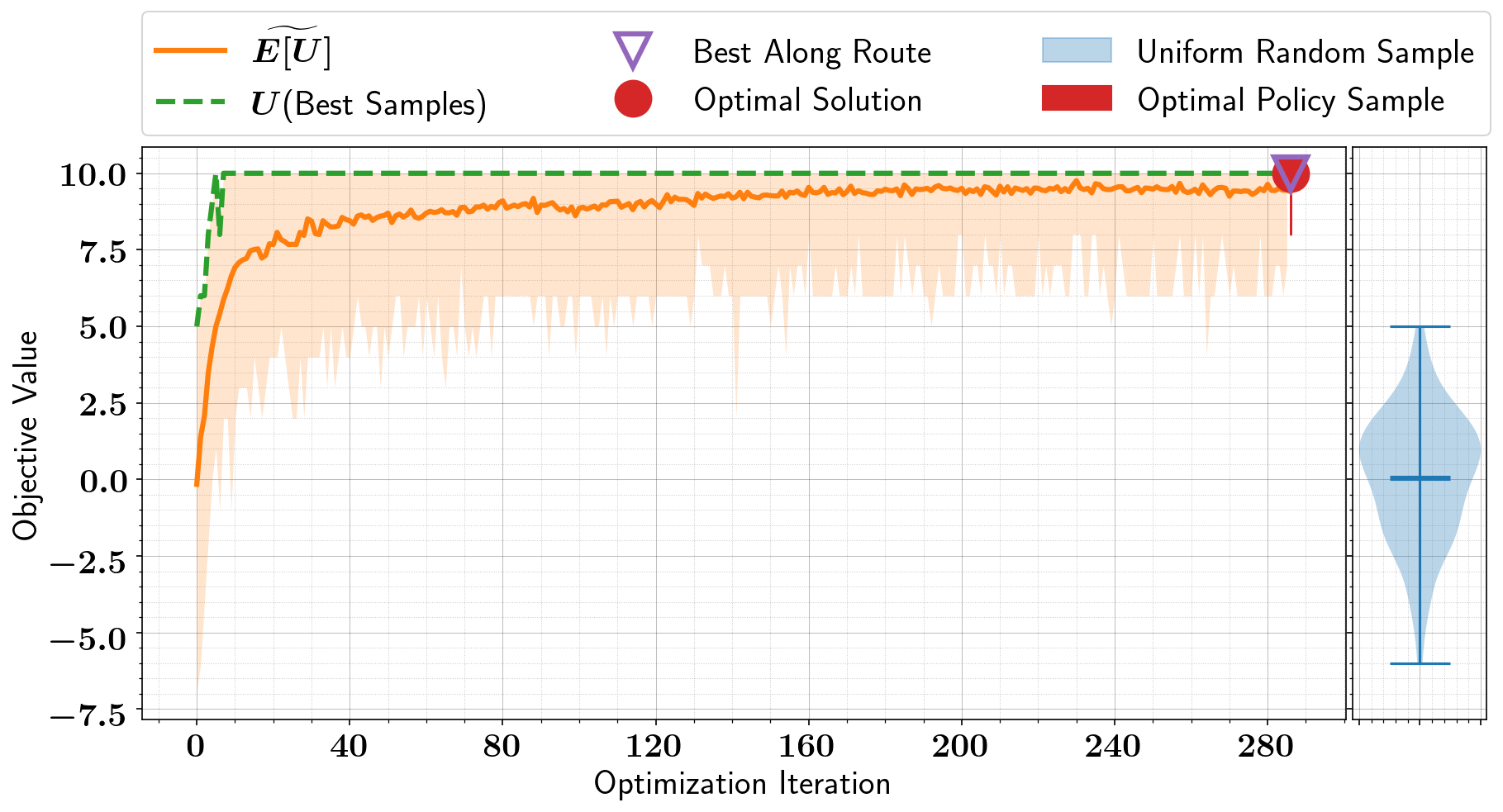
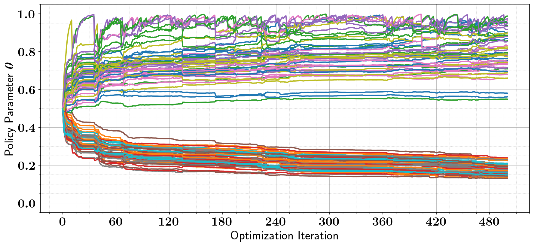
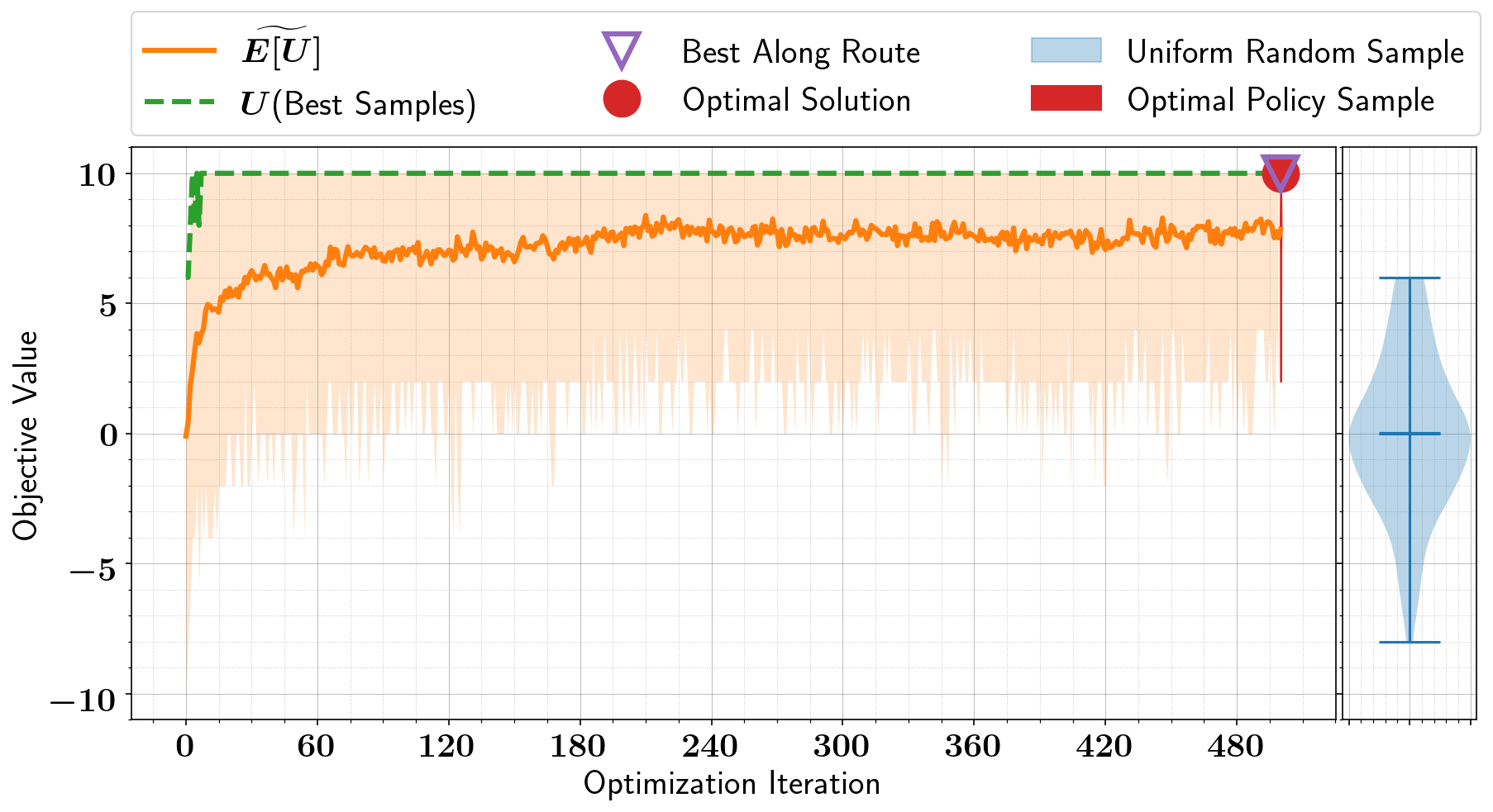
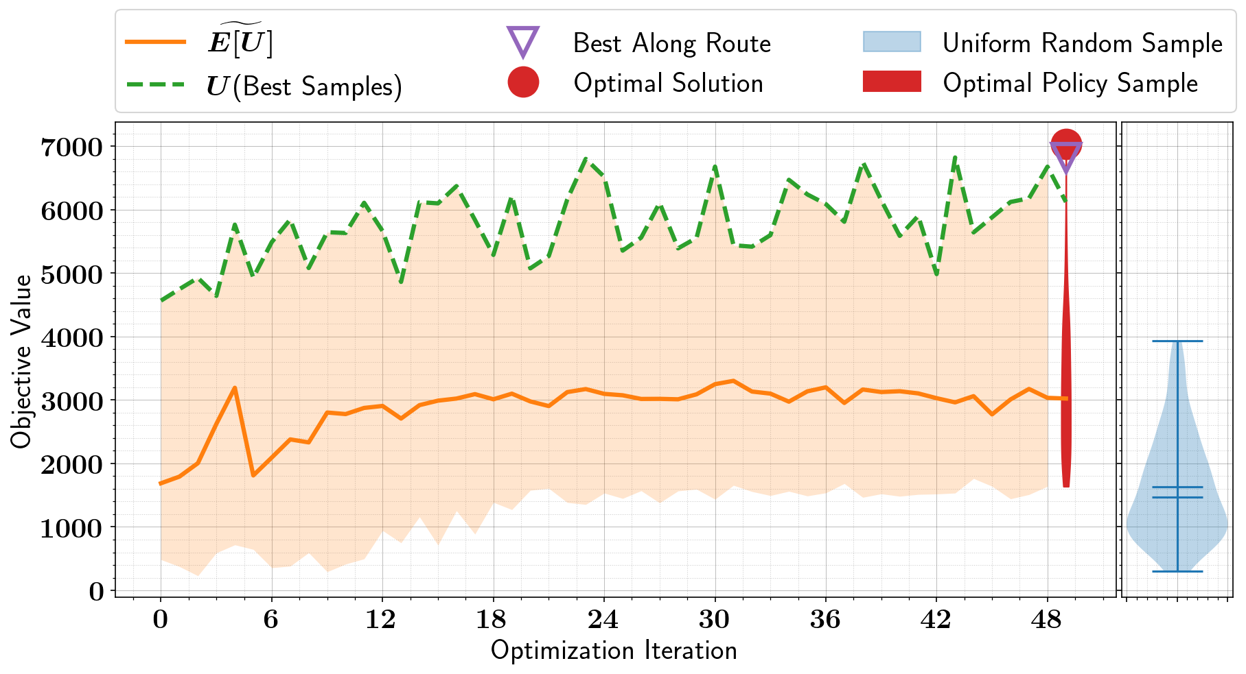
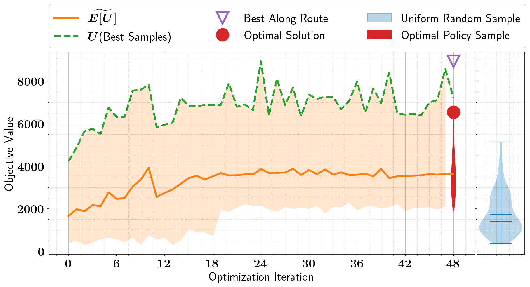
Figure 4 shows the behavior of the optimization procedure (Algorithm 3) for solving (54). Specifically, Figure 4 (left) shows the values of the best value of the objective function explored at each iteration, along with the estimate of the stochastic objective evaluated by averaging the value of over the sample used in the stochastic gradient (34). The associated violin plot shows the values of the objective corresponding to a sample of size generated assuming uniform probabilities, that is, by sampling the CB model with . This shows that the optimization procedure achieves a superior result (better than the best random sample) in just iterations. Moreover, in this case it generates an optimal solution that achieves the global maximum objective value of . We note, however, that the global optimum solution in this case is not unique. The value of the distribution parameter, that is, the success probabilities , over consecutive iterations is shown in Figure 4 (right) showing that the optimization procedure successfully and quickly identifies entries of that should be associated with higher probabilities and those that correspond to lower probabilities.
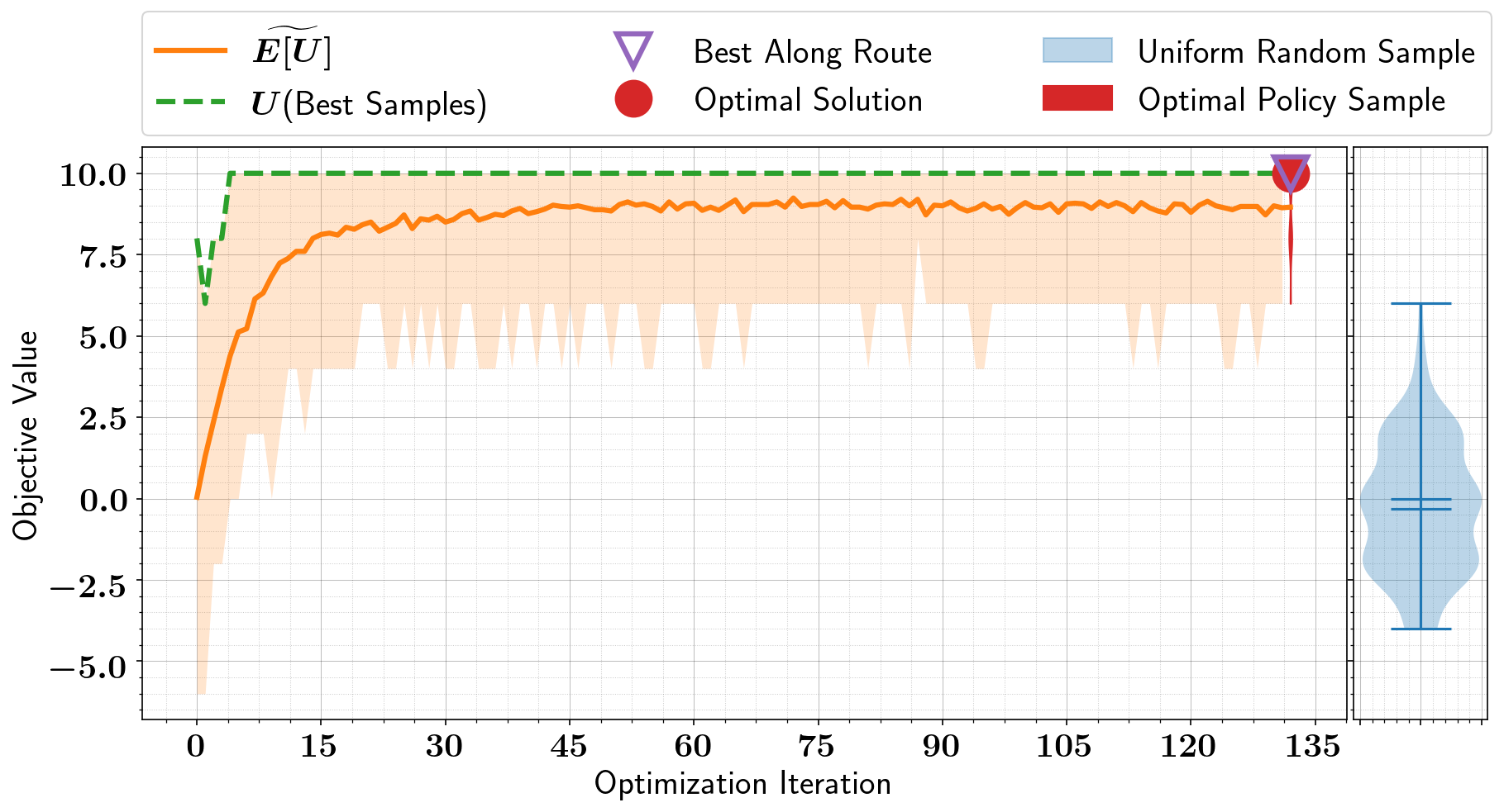

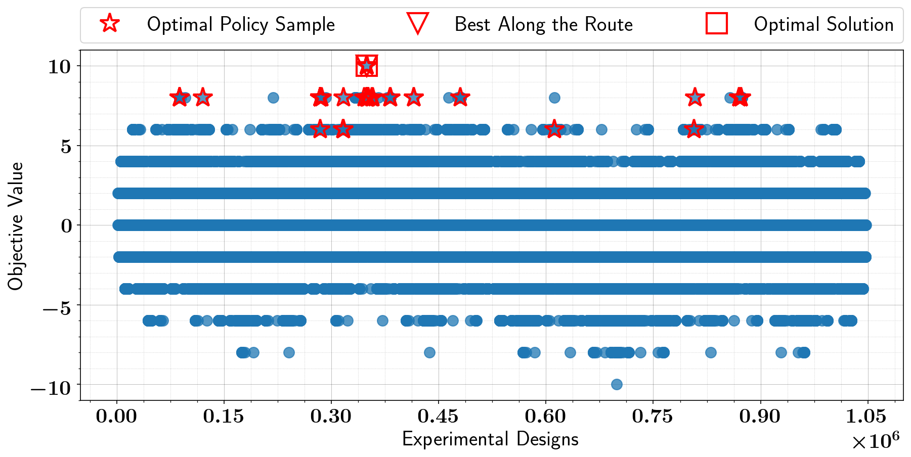
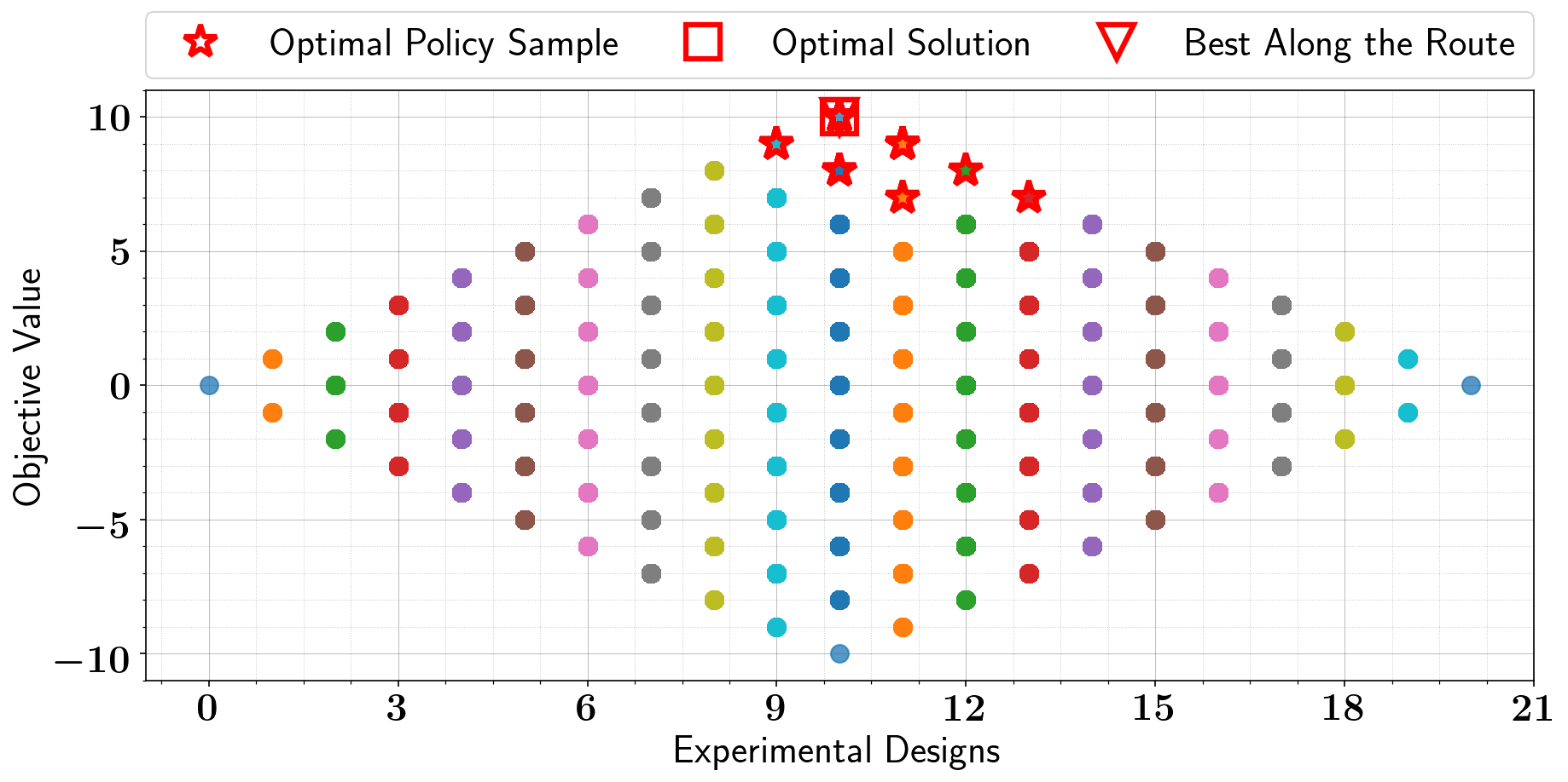
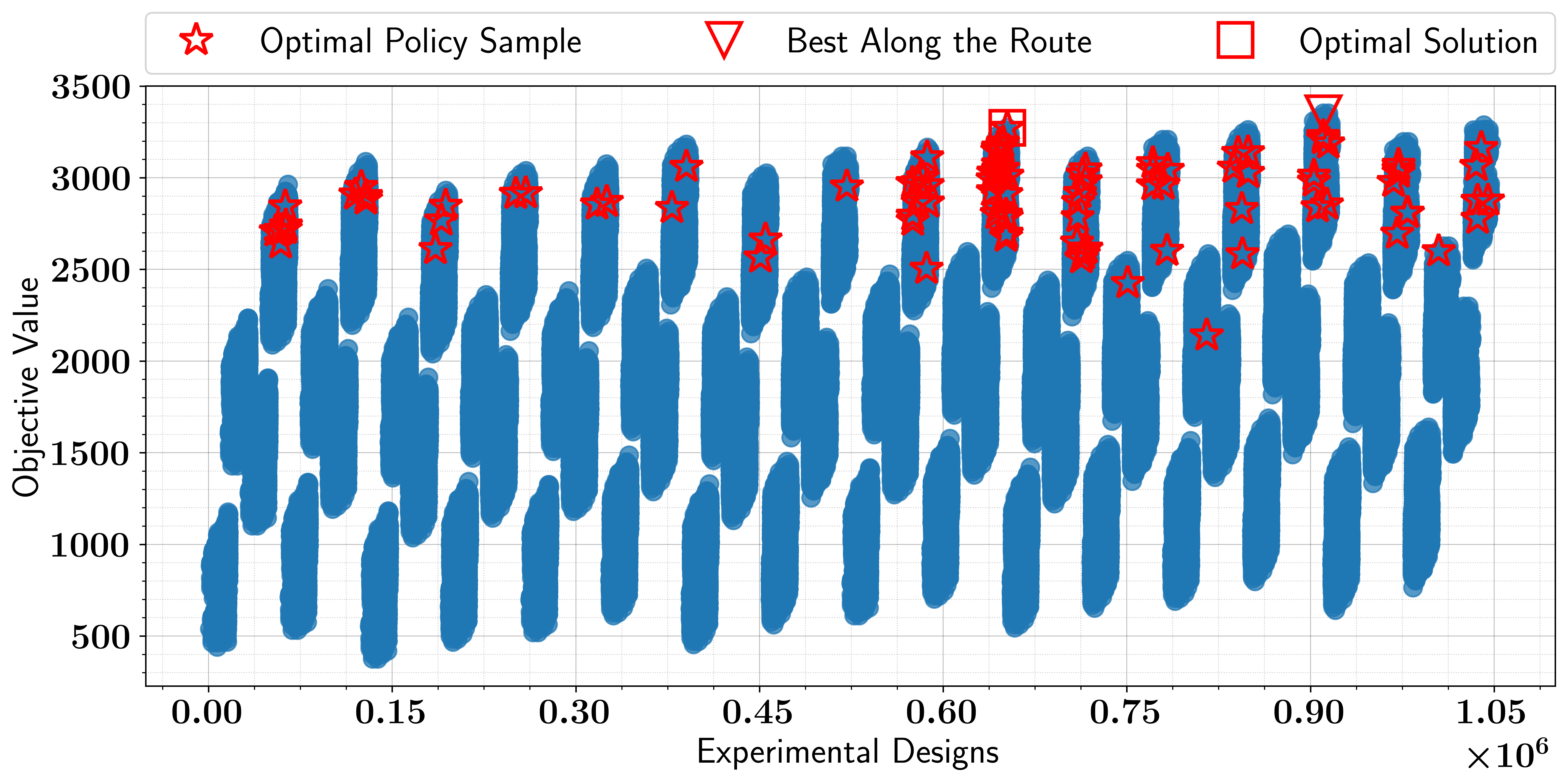
The reason Algorithm 3 did not converge to a degenerate distribution, that is, probabilities, is that the global optimum solution is nonunique and the algorithm tries to capture the distribution parameter that yields as much information about the optimal solution as possible. The sample (of size ) generated from the final policy (CB model with the final value of the parameter at the last iteration) is shown in Figure 4 compared with brute-force search over all feasible realizations of . The optimization procedure samples the optimal policy and chooses the best sample ( that achieves the maximum value of the objective ) as the optimal solution. Moreover, since the binary space is finite, the algorithm keeps track of the best value of it achieves during the exploration procedure, that is, during sampling for estimating the stochastic gradient. The result in Algorithm 3 shows that the optimal policy indeed yields samples at or near the global optimum value.
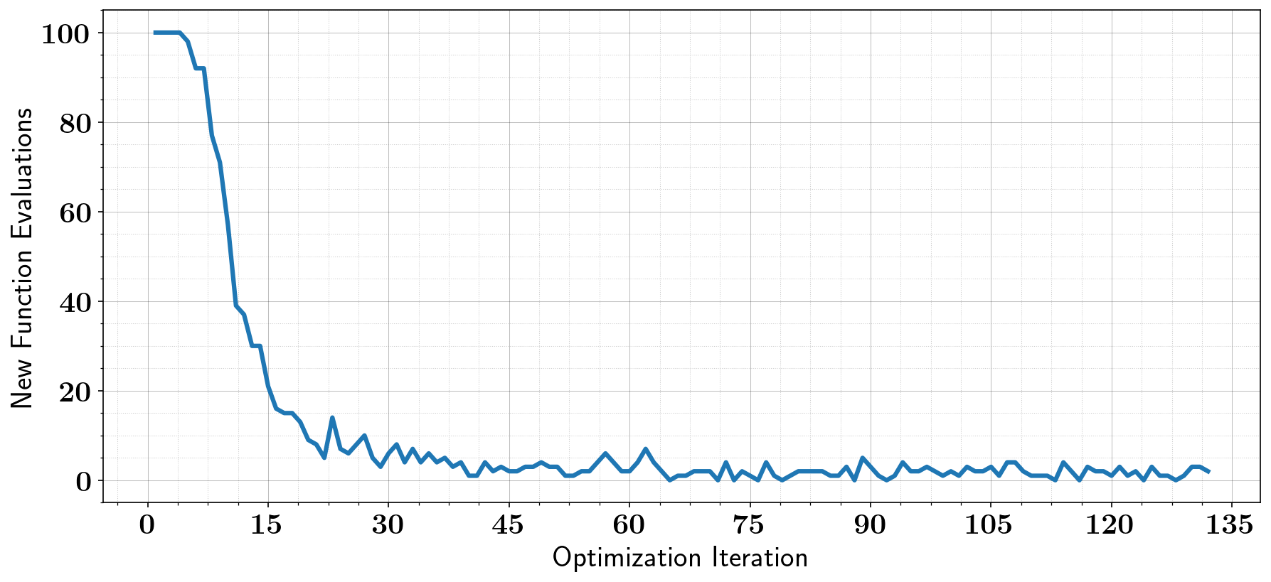
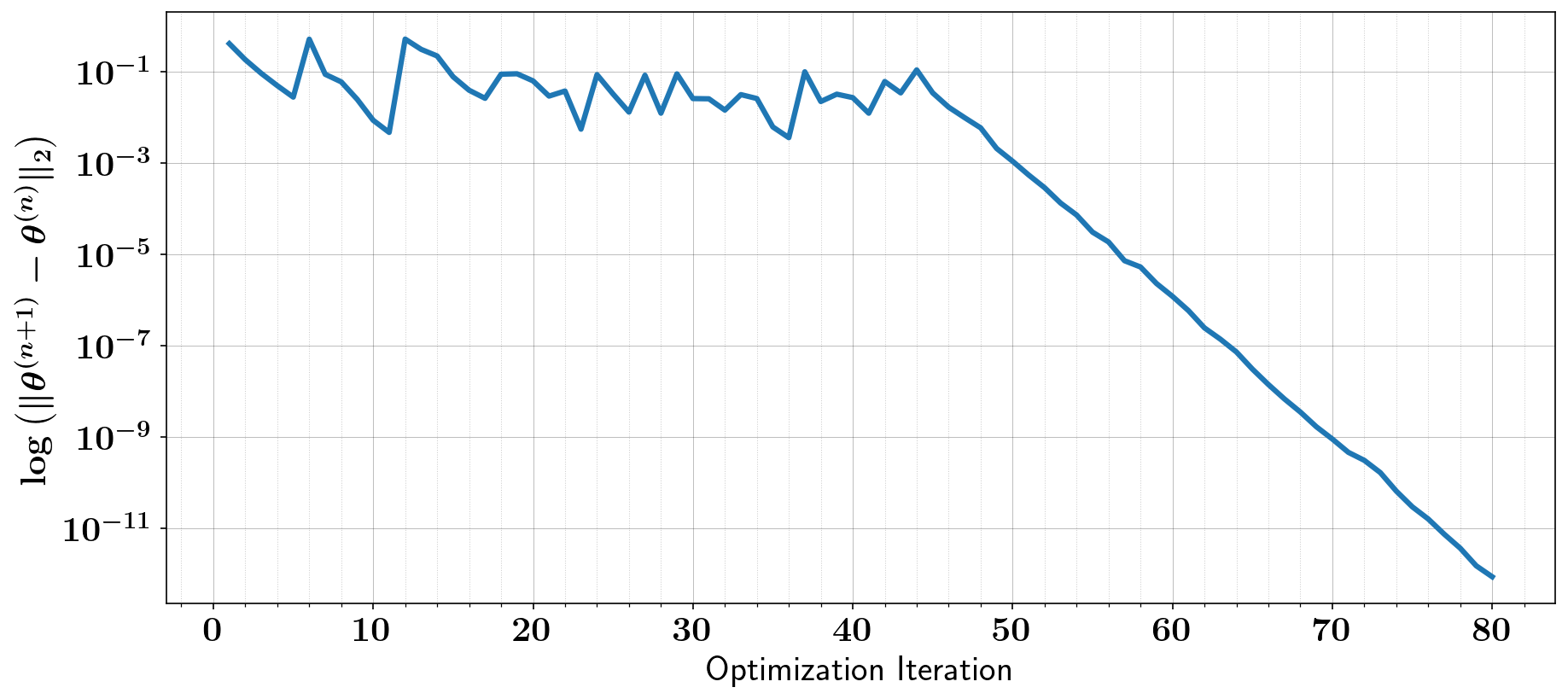
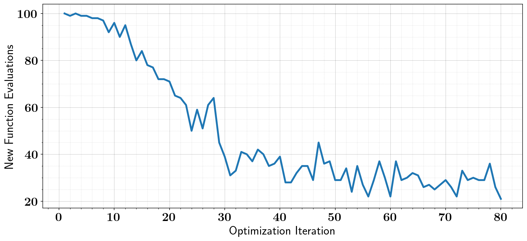
The algorithm terminates after approximately iterations; however, the major updates to the parameter happen at the first few iterations. This situation is demonstrated by Figure 4 (right) as well as Figure 6 (left), which shows the step update over consecutive iterations. Moreover, the algorithm keeps track of sampled realizations of along with the corresponding objective values . As the algorithm proceeds, the probabilities are updated and are generally pushed toward the bounds , thus promoting realizations of it has previously explored. This is demonstrated by Figure 6 (left), which shows the number of new evaluations of the objective at each iteration.

5.1.2 Results with inclusion budget constraint
We run Algorithm 3 to solve the following optimization problem:
| (55) |
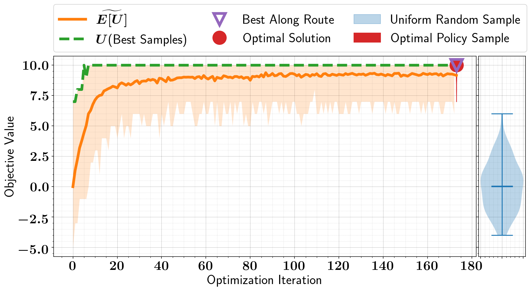
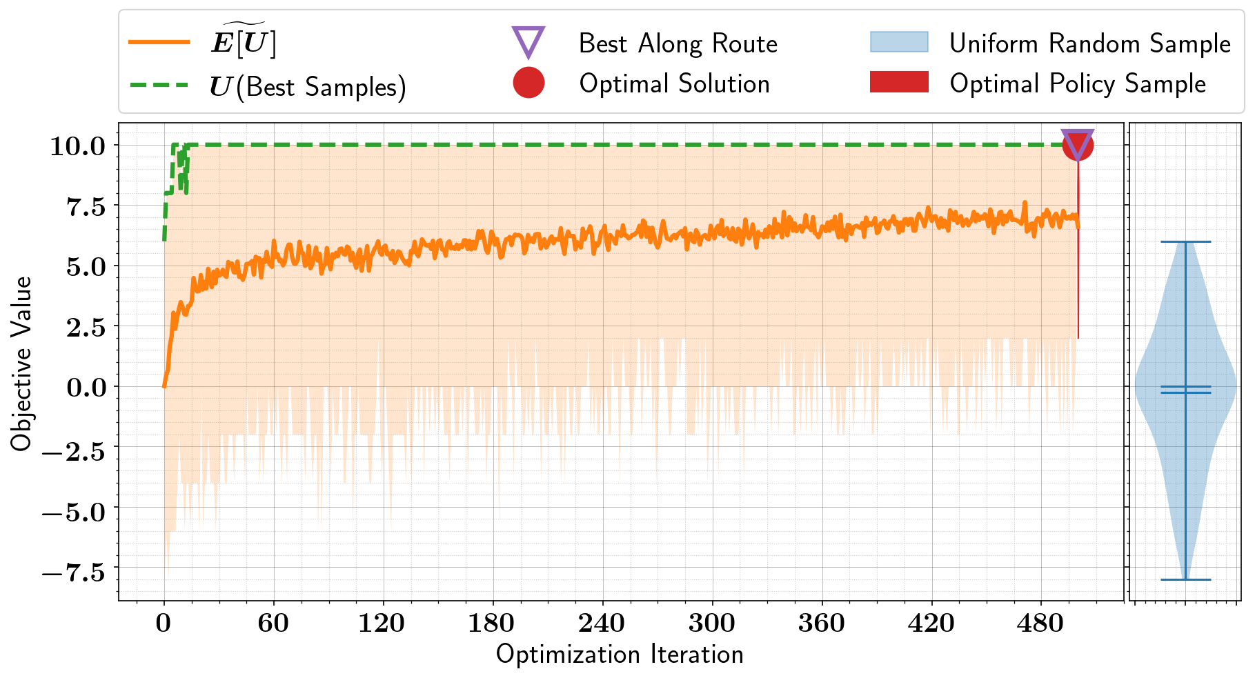
where we used the same setup as in Section 5.1.1. Here, the cardinality of the feasible region is . The algorithm shows similar performance to the results presented in Section 5.1.1 as shown in Figure 7, which shows the behavior of the optimization procedure of consecutive iterations in Figure 7 (left) and the optimization results compared with brute-force search in Figure 7 (left).

Note that the case of unconstrained binary optimization is a special case of where . Thus, we run Algorithm 3 to solve the following optimization problem:
| (56) |
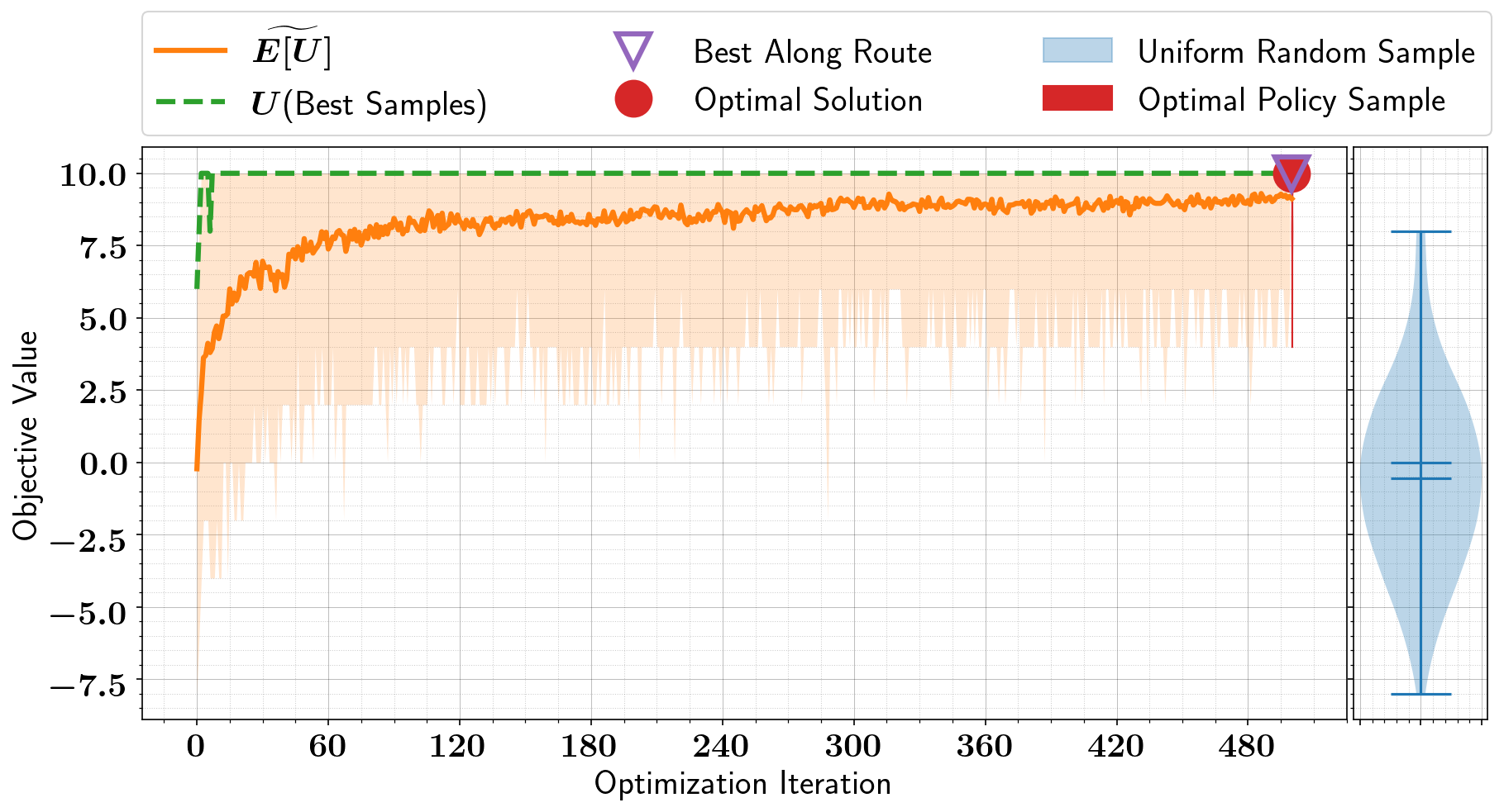
where we use the same setup as in Section 5.1.1 and Section 5.1.2 but we do not use any budget constraints. This is equivalent to setting the budget constraint to . Here, the cardinality of the feasible region is . The results are given in Figure 8 showing performance similar to that of the constrained cases.
5.1.3 Results for large dimension
To analyze the performance of the optimization Algorithm 3 for increasing cardinality (dimension of the binary variable), we show results for solving (54) for increasing dimensions. Specifically, results for are given in Figure 9, Figure 10, and Figure 11, respectively, showing performance similar to that obtained for given by Figure 4. This shows that the proposed algorithm can perform well for increasing dimensionality at the same (fixed) computational cost in terms of number of function evaluations. Note that the percentage of feasible space explored by the algorithm in the case of is .


5.2 Numerical experiments using an advection-diffusion problem
Optimal sensor placement for parameter identification using an advection-diffusion simulation model is a problem that has been used extensively in the computational science literature and has been solved by a variety of solution algorithms; see, for example, [46, 10, 11, 9]. We test our proposed approach using this problem with an experimental setup described briefly in Section 5.2.1. The numerical results are shown in Section 5.2.2.
5.2.1 Experimental setup
The advection-diffusion model (57) simulates the spatiotemporal evolution of a contaminant field in a closed domain ,
| (57) | ||||
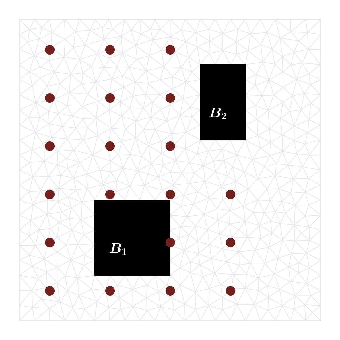
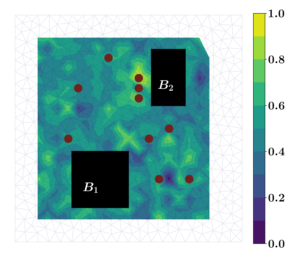
where is the diffusivity, is the simulation final time, and is the velocity field. In our experiments we set , and we employ a constant velocity field by solving a steady Navier–Stokes equation, with the side walls driving the flow [46]. The spatial domain includes two buildings (modeled as rectangular regions in the domain interior) where the flow is not allowed to enter. The domain boundary includes the external boundary and the walls of the two buildings.
The inference (inverse) problem seeks to retrieve the true (unknown) source of contamination, that is, the true initial condition given the simulation model (57) and sparse spatiotemporal observations collected from the domain at predefined sensor locations. The domain and the boundary are both shown in Figure 12 along with grid discretization and candidate sensor locations, which are discussed next.
Forward and adjoint operators
The simulation model (57) is linear. We denote the forward operator as the mapping from the inference parameter to the observation space. Thus, represents a simulation of (57) over the time interval followed by applying a restriction (observation) operator that extracts the concentration of the contaminant at all sensor locations at prespecified observation time instances. The domain is discretized following a finite-element approach, and the model adjoint is given by , where is the finite-element mass matrix.
Observational setup
Observational data is collected by using a set of uniformly distributed sensors with fixed locations in the interior of the domain . To define the optimal sensor placement OED optimization problem, we need to specify candidate senor locations where sensors are allowed to be placed. Here we consider candidate sensors (spatial distribution of sensors), respectively, with candidate sensor locations as described by Figure 12. Here the observational data (concentration of the contaminant collected by the sensors) is assumed to be collected at a set of predefined time instances with a model simulation timestep and with ; that is, we assume only observation time instances.
The observational data is corrupted with Gaussian noise , with an observation error covariance matrix . Here is the identity matrix with being the dimension of the spatiotemporal domain. We set the standard deviation of the observation error to .
The optimization problem
The optimization (optimal sensor placement) problem we are interested in solving is defined as follows:
| (58) |
where is a diagonal matrix with on its main diagonal and is the pseudo-inverse of matrix . The objective of (58) is to find the optimal placement of sensors (out of candidate locations) in the domain such that the optimal design maximizes the trace of the Fisher information matrix (FIM) defined as . Thus, the solution of (58) is an A-optimal design [49]. The numerical results of applying Algorithm 3 to solve this problem (58) are discussed in Section 5.2.2.
5.2.2 Numerical results
Results with candidate locations
Here we show results of applying Algorithm 3 to solve (58) with candidate locations as shown in Figure 12.
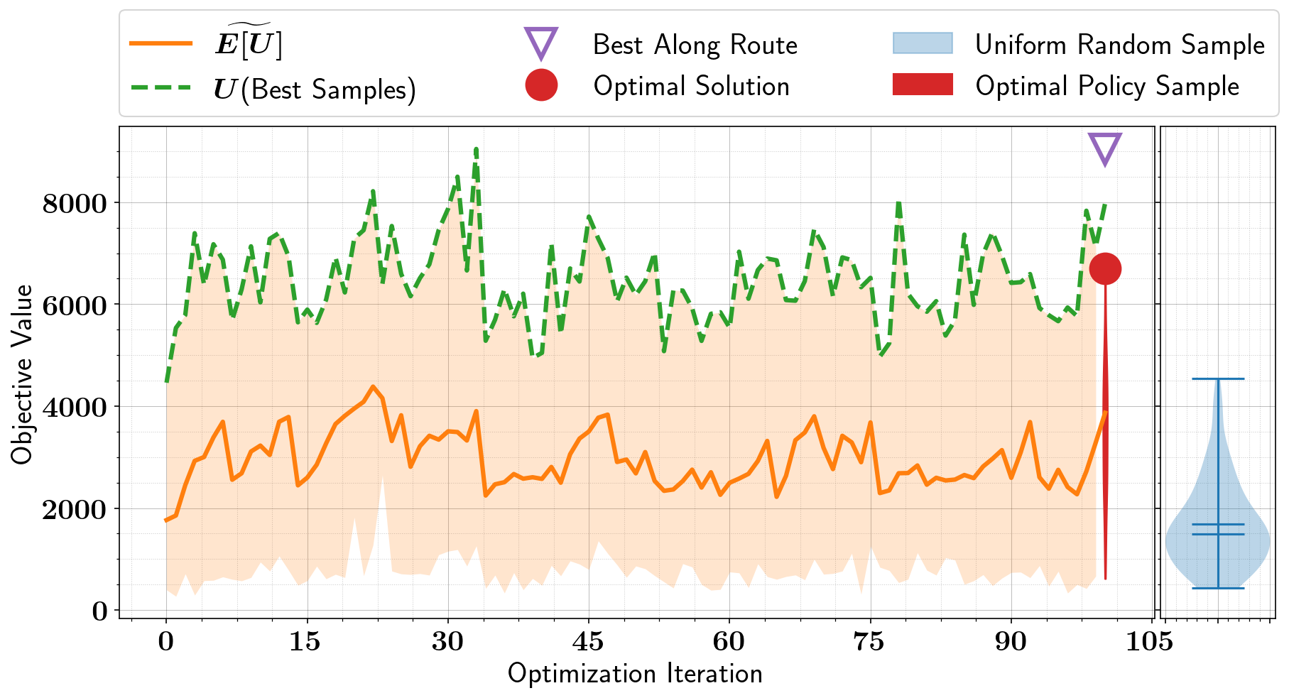
Figure 13 shows the behavior of the optimization procedure (Algorithm 3) for solving (58). The results in Figure 13 are similar to those displayed in both Figure 4 and Figure 7, respectively. As the optimization procedure iterates, the variance of the sample used to estimate the gradient (stochastic gradient estimate) reduces, indicating that the optimizer is moving toward a local optimum.
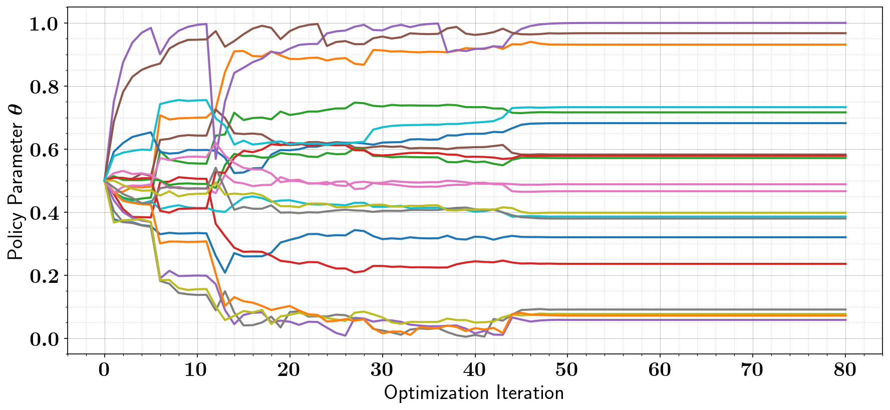
Figure 13 shows results similar to those in Figure 4. While Algorithm 3 produces results (e.g., an optimal solution estimate) slightly better than the uniformly random sample, the algorithm is able to beat the best random sample after only one iteration. Note that one iteration of the algorithm costs evaluations of the objective while the size of the uniform random sample here is set to . The superiority of the proposed approach becomes clear as the dimensionality of the problem increases as discussed below.
Similar to the results in Figure 5, the results displayed in Figure 14 show that the major updates to the parameter happen at the first few iterations and that the computational cost (number of new evaluations of the objective function ) reduces considerably as the algorithm iterates.
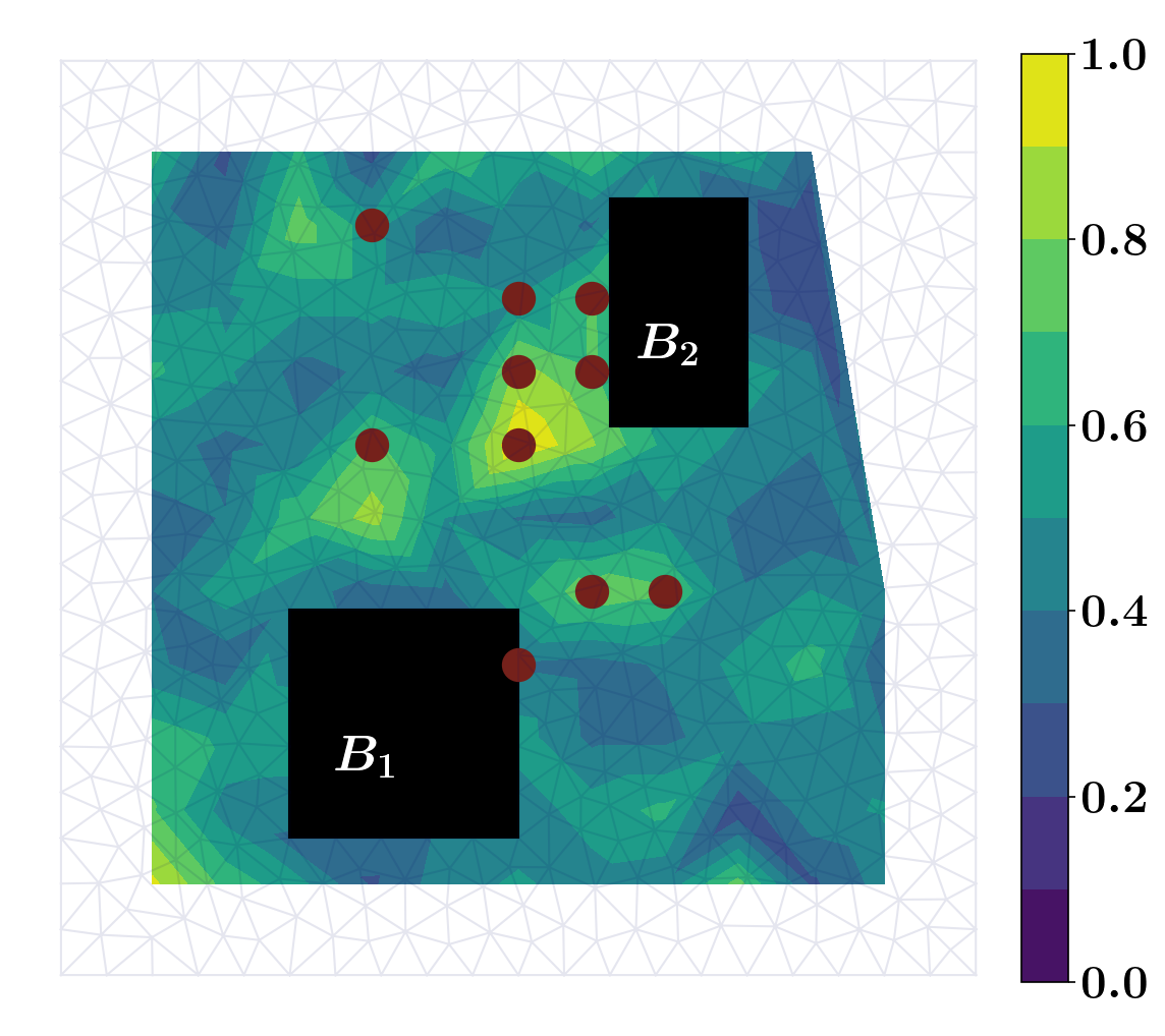
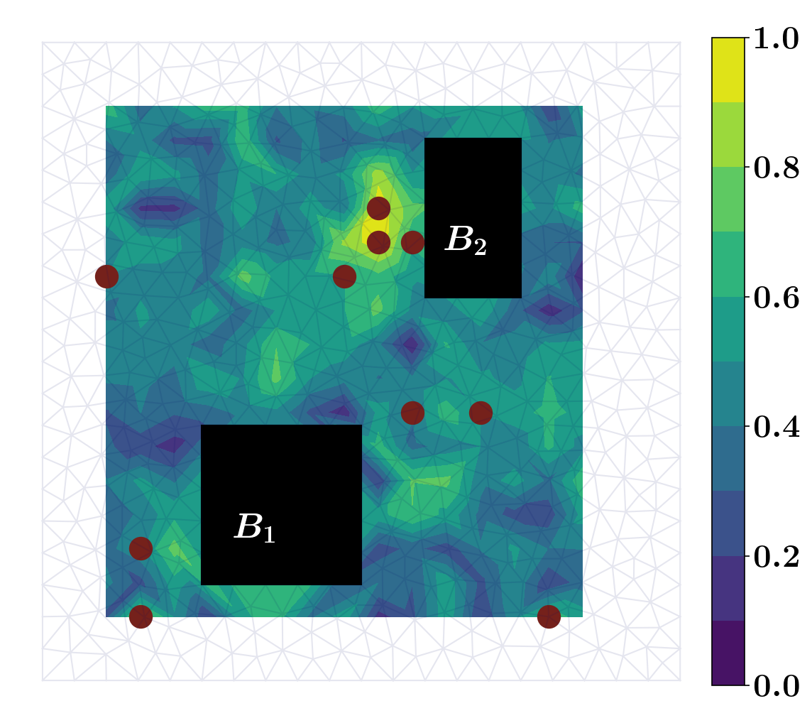
Both the optimal solution (best among the sample collected from the optimal policy) and the best solution explored by the optimization algorithm are compared with the global optimum solution in Figure 15. The sensor locations are plotted along with the value of the optimal policy parameters that is interpolated in the domain.


Here the number of design (designs with active sensors) is , which enables conducting a brute-force search to benchmark our results. Results of the optimization procedure compared with enumeration by brute-force results are shown in Figure 16. These results show that the parameters of the CB model (success probability) enable sampling a region in the feasible domain close to the global optimum. In this case the global optimum solution has been explored during the course of the optimization procedure. The optimal solution and the best along the route are very similar in structure (spatial distribution) as shown in Figure 15, and both attain very similar values of the objective function as shown in Figure 16.
Performance and scalability
Here we analyze the performance of the proposed approach for various practical scenarios. First, we discuss the algorithm results for increasing cardinality . Second, we analyze its reliability by running multiple instances to solve the same problem with different sequences of pseudorandom numbers; that is, the random seed is automatically and randomly selected by the compiler.
The results obtained for set to , , and are shown in Figure 17, Figure 18, and Figure 19, respectively. These results show consistent behaviour of the optimization procedure as the size of the problem (number of candidate sensor locations) increases. Moreover, the results show that the most likely place (highly probable) to place sensors is near the second building. The values of the CB model parameters (success probabilities) returned by the optimizer and interpolated over the domain show that the resulting policy is non-degenerate, which indicates that many candidate designs achieve an objective value near the global optimum value.


The proposed algorithm employs random samples from the CB model at each iteration as shown in Step 5 of Algorithm 3. Thus, rerunning the optimization procedure multiple times will likely yield different behavior unless a random seed of the pseudorandom number generator is set. In our experiments (and in the PyOED’s tutorials corresponding to this work), we set a fixed random seed for reproducibility of results. To analyze the reliability of the proposed approach, we show the results of applying Algorithm 3 times, each with a different random seed, for solving (58); see Figure 20.

In this experiment we set the number of candidate sensors to . Thus, the results here have the setup as those shown in Figure 17. Figure 20 shows that while the optimal design found by Algorithm 3 is not guaranteed to be the global optimum, the optimal design is much better than uniform random sampling. Moreover, since the algorithm explores the binary space without relaxation, we can keep track of the best explored sample (the sample associated with highest objective value) that the algorithm has obtained along the optimization iterations. These best along the route sample points are always at least as good as the optimal solution. Moreover, in spite of setting the maximum number of iterations to , the optimization algorithm converges quickly to a local optimum for small as well as large dimensionality.
Note that the computational cost of Algorithm 3 is predetermined by the size of the sample used in estimating the gradient (the stochastic gradient) and by the number of iterations of the optimization procedure. These results and the fact that the stochastic gradient is data parallel show that the proposed approach is computationally efficient and scalable and thus is suitable for challenging applications such as sensor placement in large-scale inverse problems and data assimilation [14, 15, 7, 13].
6 Discussion and Concluding Remarks
In this work we presented a fully probabilistic approach for binary optimization with a black-box objective function and with budget constraints. The proposed approach views the optimization variable as a random variable and employs a parametric conditional distribution to model its probability over the feasible region defined by the budget constraints. Specifically, the objective function is cast into a stochastic objective defined over the parameters of a conditional Bernoulli model, and the stochastic objective is then optimized following a stochastic gradient approach. The result is an optimal policy (parameters of the parametric distribution) that enables sampling the region at (or near) the global optimum solution(s). This is similar to stochastic policy optimization in reinforcement learning where the horizon is finite with only one time step.
The proposed approach does not require appending the objective function with a penalty term to enforce the budget constraint, as is the case with the original probabilistic optimization proposed in [11], which is ideal for unconstrained binary optimization. By using a conditional distribution whose support is restricted to the feasible region defined by the budget constraints, the proposed approach only explores (by sampling) points in the binary domain that satisfy the predefined constraints, leading to massive computational cost reduction. Note that the cost of the proposed approach in terms of number of function evaluations is predetermined by the settings of the optimization procedure, namely, by the choice of the size of the sample used to numerically evaluate the stochastic gradient, and by the number of optimization iterations. The computational cost of the proposed approach is dominated by the cost of evaluating the objective function at sampled feasible realizations of the binary variable. The proposed approach, however, is data parallel and is thus ideal for large-scale optimization problems rather than small problems where a near-optimal solution can be found, for example, by greedy methods, brute force, or even random search. Moreover, efficient inexpensive approximations of the objective function such as randomization methods and machine learning surrogates of expensive simulations can be employed to speed up the optimization process when applicable.
In this work we focused primarily on budget (cost) constraints that are popular in applications such as optimal sensor placement for computational and engineering inference problems. Modeling hard constraints using conditional probability distributions in general is a nontrivial task. General approaches such as combining Fourier transform with the characteristic function of basic distributions can help in developing conditional distributions of more complex constraints. This topic will be investigated further in future work.
The only tunable parameter in this work is the leaning rate, that is, the optimization step size. This is generally an open question for stochastic optimization with existing general guidelines such as employment of decaying learning rate schedule. In this work the domain of the optimization variable, that is, the parameters of the conditional Bernoulli model, is restricted to the hypercube . Thus, we have proposed a projection operator that works by scaling the stochastic gradient to fit within the hypercube, which enables employing a fixed learning rate (e.g., ) with encouraging empirical results. Nevertheless, automatic tuning of the learning rate will be investigated in future work, which can be applied to both the original (unconstrained) formulation and the proposed constrained probabilistic approach to binary optimization.
Appendix A Proofs of Theorems and Lemmas Discussed in Section 3
Proof A.1 (Proof of Lemma 3.1).
Given the definition of the Bernoulli weights (8), it follows that
| (59) |
where is the Kronecker delta function, that is if , and when . Thus, is a diagonal matrix with the th entry of the diagonal equal to , which proves the first relation in (9), that is, .
From (8) it follows that for each , and, for ,
| (60) |
Thus, , where is the th versor (th unit vector) in . It then follows that
| (61) |
which proves the second identity in (9), and completes the proof.
Proof A.2 (Proof of Lemma 3.3).
We prove the first identity (13a) by considering the two cases and , respectively. First, let us assume . By definition of the first order inclusion probability (11),
| (62) | ||||
Second, assume :
| (63) | ||||
The first identity (13a) is obtained by combining the two cases above. The derivative of the second-order inclusion probability (13b) similarly is as follows:
| (64) | ||||
and (13c) follows from (13b) by noting that is symmetric in both indices . The second-order derivative (13d) is then given from (13c), as follows. For ,
| (65) | ||||
which proves (13d) and completes the proof.
Proof A.3 (Proof of Lemma 3.6).
The identity (16b) follows from the definition of the R-function (8),
| (66) |
where we used (11) in the last step. The identity (16b) follows from (16a) by noting that . The last identity (16c) is obtained by applying (16a) recursively as follows; for ,
| (67) |
where we used (11) and the fact that is independent of and .
Proof A.4 (Proof of Lemma 3.9).
From (18),
| (68) | ||||
where we used the facts that in the second step, Lemma 3.1 is used in the third step, and (18) is used in the last step. This proves the first identity (19a). The second identity (19b) is a straightforward application of the rule of the logarithm derivative, , which completes the proof.
Proof A.5 (Proof of Lemma 3.12).
The first identity (21a) evaluates the PMF of the PB model when one of the success probabilities is equal to . Because we can reorder the entries of and , it is sufficient to prove the identity for . Assume , which means that the first entry of is always with probability , that is, and . By applying the law of total probability, the PMF of the PB model in this case takes the form
| (69) | ||||
which is equivalent to the PMF corresponding to removing , which is equivalent to (21a). The second identity (21b) follows similarly by considering the case where . In this case, the first entry of is always with probability . The PMF of the PB in this case is
| (70) |
which is equivalent to (21b). To prove the limits at the bounds, that is (21c), and (21d), we note that the PMF (18) can be written as follows:
| (71) | ||||
Thus the limits (21c) and (21d) are obtained by setting in the right-hand side to and , respectively. The one-sided derivatives of the PMF at the bounds are obtained as follows. The right-hand derivative at is given by
| (72) | ||||
The left-hand derivative at is similarly given by
| (73) | ||||
In this case we used the fact that . The last identity (21f) follows by noting that the the PMF of the PB model (18) can be written in the alternative form
| (74) |
Thus, the derivative with respect to takes the form
| (75) |
which is independent from and hence proves (21f).
Proof A.6 (Proof of Lemma 3.16).
We start by proving (24b). The logarithm of the CB model (23) is given by
| (76) |
Thus, the gradient of the log-PMF of the CB model (23) is given by
| (77) |
where is given by (3.1.3), and follows by definition of the weights (8),
| (78) |
where is the th unit vector in . Thus,
| (79) | ||||
where vector operations are computed elementwise, that is, , and is the th versor (unit vector) in . The identity (24a) follows by noting that and by using (24b), and (23), respectively.
Proof A.7 (Proof of Lemma 3.18).
Proof A.8 (Proof of Lemma 3.20).
While in [24] it was noted that the first identity holds, the proof was not accessible. Thus, we provide the proof here in detail for completeness. Using the formula of expectation,
| (82) |
we can extract the components of the conditional expectation,
| (83) | ||||
which proves (26a). Similarly the second identity(26b) is obtained as follows. Assuming , we have
| (84) | ||||
where the second step is obtained by dropping all terms with or from the expectation expansion. In the other case, namely , since , we have and thus for we have which proves the second identity (26b). The third identity (26c) follows from both (26a) and (26b), since . The identity (26d) is obtained as follows
| (85) | ||||
where is the th unit vector in . The identity (26e) then follows by using (26d) and (25a) and by summing the variances of the entries of as follows:
| (86) | ||||
where we used the fact that in the last step, which completes the proof.
Proof A.9 (Proof of Lemma 3.22).
The two identities (27a) and (27b) describe the PMF of the conditional Bernoulli model at the boundary of the probability domain, that is, at and , respectively. To prove these two identities, we note that the PMF of the CB model (23) takes the following equivalent form,
| (87) | ||||
which is the product of two terms. The first term is the PMF of a CB model obtained by discarding the th component of , and the second component is the first-order inclusion probability ; see Section 3.1.1. Assuming , then
| (88) |
which shows that the value of the PMF (23) is equal to when , which is intuitively expected. If we let , then the first term in the product (87) is given by
| (89) | ||||
which together with (87) proves (27a). Similarly, for ,
| (90) | ||||
which together with (87) proves (27b). To prove the limits (27c) and (27d), we write the PMF of the CB model (23) as follows:
| (91) | ||||
Thus, for ,
| (92) | ||||
| (93) |
and for ,
| (94) | ||||
| (95) |
which proves (27d). The right-hand derivative (27e) at can be defined as
| (96) |
which, by letting , can be equivalently written (by replacing with ) as
| (97) | ||||
which proves (27e) for . Similarly, for ,
| (98) | ||||
which completes the proof of (27e). The left derivative (27f) can be shown by following the same procedure as above for proving (27f),
| (99) |
By letting , the left derivative at is given by
| (100) | ||||
and for
| (101) | ||||
which completes the proof of (27f).
The continuity of the derivative at the bounds and given by (27g) and (27h), respectively, is obtained by taking the limit of the PMF model derivative (25b) as approaches these respective limits. Specifically, for any
| (102) | ||||
By setting , it follows that
| (103) | ||||
and
| (104) | ||||
For ,
| (105) | ||||
and,
| (106) | ||||
which proves continuity of the derivative of the CB model over the domain and completes the proof.
Proof A.10 (Proof of Lemma 3.26).
By the definition of Bayes’ rule and the conditional probability, it follows that
| (107) |
and, because realizations of the sum are mutually exclusive, that is, cannot take different values at the same time, then , , hence for any two realizations of . Thus by using (107), we have
| (108) | ||||
which completes the proof of (29a). The identity (29b) is obtained from (29a) as follows,
| (109) | ||||
which proves (29b). (29c) follows from (29b) and by using the definition of the derivative of the logarithmic function. By the definition of the conditional expectation and by using (29a), we have
| (110) | ||||
which proves (29d). Similarly, by the definition of the conditional variance and by using (29d) it follows that
| (111) | ||||
which is equivalent to (29e) and thus completes the proof.
Appendix B Proofs of Theorems and Lemmas Discussed in Section 4
Proof B.1 (Proof of Theorem 4.3).
The first bound (49a) is given by
| (112) | ||||
where ; we used the fact that is constant for all terms in the sum in the second step; is used in the third step; and because , it follows that , and , which is used in the final step. The second bound (49b) is obtained by using (26d) and (26e), as follows:
| (113) | ||||
where we used linearity and the circular property of the trace operator in the first step. Since for the first-order inclusion probabilities satisfy and since is a quadratic with maximum value , it follows from (113) that
| (114) |
which proves (49b). To prove (49c), we use (25c) and note that and , and from (12) it follows that . Thus,
| (115) | ||||
where we used the facts that and in the second step. This completes the proof of (49c).
To prove the bounds in the general case of of non-degenerate probabilities, we note that (28c) is equivalent to (25b) for the first case . In each of the other degenerate cases in (28c), the derivatives are expressed in terms of the weights of the non-degenerate parts. Thus, from (49) it follows that there is always a finite number (defined based on the maximum/minimum success probability ) that bounds first- and second-order derivatives. This proves (49) and completes the proof of the theorem.
Proof B.2 (Proof of Theorem 4.5 ).
| (116) | ||||
which proves (50a). For any two realizations of the CB model parameters , it follows that
| (117) |
which proves (50b). The bound on the Hessian entries (50c) are obtained as follows:
| (118) | ||||
which by taking the square roots on both sides proves (50c). The boundedness of the derivatives (51) follows immediately from (50) and (49d).
Proof B.3 (Proof of Theorem 4.7 ).
| (119) | ||||
which proves that the stochastic approximation is an unbiased estimator of the exact gradient of the stochastic objective . The second identity in (52b) is obtained as follows:
| (120) | ||||
where . By Theorem 4.3, there is a positive finite constant such that , which completes the proof of (52b) and the theorem.
References
- [1] A. Alexanderian, Optimal experimental design for Bayesian inverse problems governed by PDEs: A review, arXiv preprint arXiv:2005.12998, (2020).
- [2] A. Alexanderian, P. J. Gloor, O. Ghattas, et al., On Bayesian A-and D-optimal experimental designs in infinite dimensions, Bayesian Analysis, 11 (2016), pp. 671–695.
- [3] A. Alexanderian, N. Petra, G. Stadler, and O. Ghattas, A-optimal design of experiments for infinite-dimensional Bayesian linear inverse problems with regularized -sparsification, SIAM Journal on Scientific Computing, 36 (2014), pp. A2122–A2148, https://doi.org/10.1137/130933381.
- [4] A. Alexanderian, N. Petra, G. Stadler, and O. Ghattas, A fast and scalable method for A-optimal design of experiments for infinite-dimensional Bayesian nonlinear inverse problems, SIAM Journal on Scientific Computing, 38 (2016), pp. A243–A272, https://doi.org/10.1137/140992564, http://dx.doi.org/10.1137/140992564.
- [5] A. Alexanderian, N. Petra, G. Stadler, and I. Sunseri, Optimal design of large-scale Bayesian linear inverse problems under reducible model uncertainty: good to know what you don’t know, SIAM/ASA Journal on Uncertainty Quantification, 9 (2021), pp. 163–184.
- [6] A. Alexanderian and A. K. Saibaba, Efficient D-optimal design of experiments for infinite-dimensional Bayesian linear inverse problems, Submitted, (2017), https://arxiv.org/abs/1711.05878.
- [7] A. Attia, Advanced Sampling Methods for Solving Large-Scale Inverse Problems, PhD thesis, Virginia Tech, 2016.
- [8] A. Attia, PyOED: An extensible suite for data assimilation and model-constrained optimal design of experiments, 2024, https://gitlab.com/ahmedattia/pyoed.
- [9] A. Attia, A. Alexanderian, and A. K. Saibaba, Goal-oriented optimal design of experiments for large-scale Bayesian linear inverse problems, Inverse Problems, 34 (2018), p. 095009.
- [10] A. Attia and E. Constantinescu, Optimal experimental design for inverse problems in the presence of observation correlations, SIAM Journal on Scientific Computing, 44 (2022), pp. A2808–A2842.
- [11] A. Attia, S. Leyffer, and T. Munson, Stochastic learning approach for binary optimization: Application to Bayesian optimal design of experiments, SIAM Journal on Scientific Computing, 44 (2022), pp. B395–B427.
- [12] A. Attia, S. Leyffer, and T. Munson, Robust a-optimal experimental design for bayesian inverse problems, 2023, https://arxiv.org/abs/2305.03855.
- [13] A. Attia, A. Moosavi, and A. Sandu, Cluster sampling filters for non-Gaussian data assimilation, Atmosphere, 9 (2018), https://doi.org/10.3390/atmos9060213.
- [14] A. Attia, V. Rao, and A. Sandu, A sampling approach for four dimensional data assimilation, in Dynamic Data-Driven Environmental Systems Science, Springer, 2015, pp. 215–226.
- [15] A. Attia, V. Rao, and A. Sandu, A hybrid Monte Carlo sampling smoother for four dimensional data assimilation, International Journal for Numerical Methods in Fluids, (2016), https://doi.org/10.1002/fld.4259. fld.4259.
- [16] A. Attia and A. Sandu, A hybrid Monte Carlo sampling filter for non-Gaussian data assimilation, AIMS Geosciences, 1 (2015), pp. 41–78, https://doi.org/http://dx.doi.org/10.3934/geosci.2015.1.41.
- [17] A. Attia, R. Ştefănescu, and A. Sandu, The reduced-order hybrid Monte Carlo sampling smoother, International Journal for Numerical Methods in Fluids, (2016), https://doi.org/10.1002/fld.4255. fld.4255.
- [18] R. Bannister, A review of operational methods of variational and ensemble-variational data assimilation, Quarterly Journal of the Royal Meteorological Society, 143 (2017), pp. 607–633.
- [19] M. G. Bellemare, W. Dabney, and M. Rowland, Distributional reinforcement learning, MIT Press, 2023.
- [20] D. P. Bertsekas and J. Tsitsiklis, Neuro–Dynamic Programming, Athena Scientific, Belmont, Massachusetts, 1996.
- [21] D. P. Bertsekas and J. N. Tsitsiklis, Neuro-dynamic programming, Athena Scientific, 1996.
- [22] Y. Boykov, O. Veksler, and R. Zabih, Fast approximate energy minimization via graph cuts, IEEE Transactions on Pattern Analysis and Machine Intelligence, 23 (2001), pp. 1222–1239.
- [23] E. Y. Chan and D.-Y. Yeung, A convex formulation of modularity maximization for community detection, in Proceedings of the Twenty-Second International Joint Conference on Artificial Intelligence (IJCAI), Barcelona, Spain, 2011, p. 2218.
- [24] S. X. Chen, General properties and estimation of conditional Bernoulli models, Journal of Multivariate Analysis, 74 (2000), pp. 69–87.
- [25] S. X. Chen and J. S. Liu, Statistical applications of the Poisson-binomial and conditional Bernoulli distributions, Statistica Sinica, (1997), pp. 875–892.
- [26] A. Chowdhary, S. E. Ahmed, and A. Attia, PyOED: An extensible suite for data assimilation and model-constrained optimal design of experiments, ACM Transactions on Mathematical Software, (2024), https://doi.org/10.1145/3653071, https://doi.org/10.1145/3653071. Just Accepted.
- [27] R. Daley, Atmospheric data analysis, Cambridge University Press, 1991.
- [28] M. A. Davenport, Y. Plan, E. Van Den Berg, and M. Wootters, 1-bit matrix completion, Information and Inference: A Journal of the IMA, 3 (2014), pp. 189–223.
- [29] D. C. Elton, Z. Boukouvalas, M. D. Fuge, and P. W. Chung, Deep learning for molecular design—a review of the state of the art, Molecular Systems Design & Engineering, 4 (2019), pp. 828–849.
- [30] V. Fedorov and J. Lee, Design of experiments in statistics, in Handbook of semidefinite programming, R. S. H. Wolkowicz and L. Vandenberghe, eds., vol. 27 of Internat. Ser. Oper. Res. Management Sci., Kluwer Acad. Publ., Boston, MA, 2000, pp. 511–532.
- [31] M. Frangos, Y. Marzouk, K. Willcox, and B. van Bloemen Waanders, Surrogate and Reduced-Order Modeling: A Comparison of Approaches for Large-Scale Statistical Inverse Problems, John Wiley & Sons, Ltd, 2010, ch. 7, pp. 123–149, https://doi.org/https://doi.org/10.1002/9780470685853.ch7, https://onlinelibrary.wiley.com/doi/abs/10.1002/9780470685853.ch7, https://arxiv.org/abs/https://onlinelibrary.wiley.com/doi/pdf/10.1002/9780470685853.ch7.
- [32] E. Haber, L. Horesh, and L. Tenorio, Numerical methods for experimental design of large-scale linear ill-posed inverse problems, Inverse Problems, 24 (2008), pp. 125–137.
- [33] L. He, C.-T. Lu, J. Ma, J. Cao, L. Shen, and P. S. Yu, Joint community and structural hole spanner detection via harmonic modularity, in Proceedings of the 22nd ACM SIGKDD International Conference on Knowledge Discovery and Data Mining, 2016, pp. 875–884.
- [34] J. Heng, P. E. Jacob, and N. Ju, A simple Markov chain for independent Bernoulli variables conditioned on their sum, arXiv preprint arXiv:2012.03103, (2020).
- [35] S. Howard, Discussion on Professor Cox’s paper, Journal of the Royal Statistical Society, Series B, 34 (1972), pp. 210–211.
- [36] J. Keuchel, C. Schnorr, C. Schellewald, and D. Cremers, Binary partitioning, perceptual grouping, and restoration with semidefinite programming, IEEE Transactions on Pattern Analysis and Machine Intelligence, 25 (2003), pp. 1364–1379.
- [37] K. Koval, A. Alexanderian, and G. Stadler, Optimal experimental design under irreducible uncertainty for linear inverse problems governed by pdes, Inverse Problems, (2020).
- [38] D. P. Kroese, T. Taimre, and Z. I. Botev, Handbook of Monte Carlo methods, John Wiley & Sons, 2013.
- [39] C. L. Lawson and R. J. Hanson, Solving least squares problems, SIAM, 1995.
- [40] J. H. Lubin, An empirical evaluation of the use of conditional and unconditional likelihoods for case-control data, Biometrika, 68 (1981), pp. 567–571.
- [41] K. Miller, Least squares methods for ill-posed problems with a prescribed bound, SIAM Journal on Mathematical Analysis, 1 (1970), pp. 52–74.
- [42] I. M. Navon, Data assimilation for numerical weather prediction: a review, in Data assimilation for atmospheric, oceanic and hydrologic applications, Springer, 2009, pp. 21–65.
- [43] J. Nocedal and S. Wright, Numerical optimization, Springer Science & Business Media, 2006.
- [44] T. P. Papalexopoulos, C. Tjandraatmadja, R. Anderson, J. P. Vielma, and D. Belanger, Constrained discrete black-box optimization using mixed-integer programming, in International Conference on Machine Learning, PMLR, 2022, pp. 17295–17322.
- [45] A. Pázman, Foundations of optimum experimental design, D. Reidel Publishing Co., 1986.
- [46] N. Petra and G. Stadler, Model variational inverse problems governed by partial differential equations, Tech. Report 11-05, The Institute for Computational Engineering and Sciences, The University of Texas at Austin, 2011.
- [47] A. Pradhan and H. S. Dhillon, Novel probabilistic reformulation technique for unconstrained discrete RIS optimization, in 2023 IEEE 34th Annual International Symposium on Personal, Indoor and Mobile Radio Communications (PIMRC), IEEE, 2023, pp. 1–6.
- [48] A. Pradhan and H. S. Dhillon, A probabilistic reformulation technique for discrete ris optimization in wireless systems, IEEE Transactions on Wireless Communications, (2023).
- [49] F. Pukelsheim, Optimal design of experiments, John Wiley & Sons, New York, 1993.
- [50] M. Ryu, A. Attia, A. Barnes, R. Bent, S. Leyffer, and A. Mate, Heuristic algorithms for placing geomagnetically induced current blocking devices, arXiv preprint arXiv:2310.09409, (2023).
- [51] J. Shi and J. Malik, Normalized cuts and image segmentation, IEEE Transactions on Pattern Analysis and Machine Intelligence, 22 (2000), pp. 888–905.
- [52] X. Shi, H. Ling, J. Xing, and W. Hu, Multi-target tracking by rank-1 tensor approximation, in Proceedings of the IEEE Conference on Computer Vision and Pattern Recognition, 2013, pp. 2387–2394.
- [53] A. Sunter, Solutions to the problem of unequal probability sampling without replacement, International Statistical Review/Revue Internationale de Statistique, (1986), pp. 33–50.
- [54] D. Uciński, Optimal sensor location for parameter estimation of distributed processes, International Journal of Control, 73 (2000), pp. 1235–1248.
- [55] J. Wang, W. Liu, S. Kumar, and S.-F. Chang, Learning to hash for indexing big data—a survey, Proceedings of the IEEE, 104 (2015), pp. 34–57.
- [56] L. A. Wolsey and G. L. Nemhauser, Integer and combinatorial optimization, John Wiley & Sons, 2014.
- [57] K. K. Yang, Z. Wu, and F. H. Arnold, Machine-learning-guided directed evolution for protein engineering, Nature Methods, 16 (2019), pp. 687–694.
- [58] J. Yu, V. M. Zavala, and M. Anitescu, A scalable design of experiments framework for optimal sensor placement, Journal of Process Control, 67 (2018), pp. 44–55.
- [59] X.-T. Yuan and T. Zhang, Truncated power method for sparse eigenvalue problems, Journal of Machine Learning Research, 14 (2013).
The submitted manuscript has been created by UChicago Argonne, LLC, Operator of Argonne National Laboratory (“Argonne”). Argonne, a U.S. Department of Energy Office of Science laboratory, is operated under Contract No. DE-AC02-06CH11357. The U.S. Government retains for itself, and others acting on its behalf, a paid-up nonexclusive, irrevocable worldwide license in said article to reproduce, prepare derivative works, distribute copies to the public, and perform publicly and display publicly, by or on behalf of the Government. The Department of Energy will provide public access to these results of federally sponsored research in accordance with the DOE Public Access Plan. http://energy.gov/downloads/doe-public-access-plan.