An information geometric probe for charged black holes in 4D Einstein-Gauss-Bonnet gravity

Abstract

Glavan and Lin [Phys. Rev. Lett. 124, 081301 (2020)] have recently proposed a consistent model of Einstein-Gauss-Bonnet modified gravity in four spacetime dimensions. This model predicts significant contributions of the Gauss-Bonnet coupling parameter $\alpha$ to gravitational dynamics, while circumventing the Lovelock theorem and avoiding Ostrogradsky instability. As a powerful competitor to general relativity, the model has been examined on various phenomenological grounds. Here, we employ a technique from thermodynamic geometry to analyze the thermodynamic phase structure of a charged black hole with a quantum gravity-inspired entropy relation in this novel modified gravity scenario. Based on the sign and magnitude of thermodynamic curvature, we demonstrate that while the theory does not significantly impact larger black holes, it may lead to multiple phase transitions and accelerate the formation of black hole remnants at short-distance scales compared to general relativity. Our analysis focuses solely on the non-extremal geometry case where $M>\sqrt{Q^{2}+\alpha}$, with $M$ and $Q$ representing the mass and charge of the black hole, respectively. We believe that these results may offer insights for testing the phenomenological consistency of the theory as a potential alternative to the standard Einstein paradigm.

I Introduction

The pioneering works of Hawking Hawking (1974, 1975) and Bekenstein Bekenstein (1973) laid the foundation for the thermodynamics of black holes, establishing a crucial cornerstone in the modern understanding of our Universe. The conventional Bekenstein-Hawking formulation necessitates an entropy-area correspondence, mathematically represented by $S_{\rm BH}=A/(4\ell_{\rm p}^{2})$, where $A$ is the horizon area and $\ell_{\rm p}$ the Planck length. The fact that black hole entropy scales with its area rather than its volume is the foundation of the holographic principle Susskind (1995); Bousso (2003). This paradigm effectively describes black hole thermodynamic behavior in terms of macroscopic parameters (e.g., mass, charge, and angular momentum). However, it does not provide insight into the underlying thermodynamic degrees of freedom. Consequently, despite being considered perfect thermal systems, black hole thermodynamics remains not fully understood Davies (1978); Page (2005). Drawing insights from Boltzmann’s principle, “If you can heat it, it has microscopic structure”, which has greatly guided our understanding of the microstructure of thermodynamic systems, we naturally confront the question: is it possible to decipher some kind of micromolecules (whatever they may look like!) that give rise to what the Bekenstein-Hawking formulation envisions for a black hole? Our work attempts to address this question within a novel modified gravity framework going beyond the Einstein paradigm.

It is well-known that Hawking evaporation Hawking (1974, 1975) is based on a semiclassical foundation, where spacetime geometry is described by classical Einstein equations. This process reduces a black hole’s size, and a quantum gravity theory is needed to describe the geometry once a characteristic size is reached. Quantum gravity theories predict a minimum measurable distance scale in nature, beyond which classical geometry breaks down due to quantum fluctuations Hossenfelder (2013). This naturally challenges the Bekenstein-Hawking formulation Mann and Solodukhin (1998); Upadhyay et al. (2018); Pourhassan et al. (2020). As the geometric description changes, so does the Bekenstein-Hawking entropy, leading us to compute black hole microstates Strominger and Vafa (1996).

The modification of Bekenstein-Hawking entropy is tied to the quantum gravity scale in string theories or loop quantum gravity, and these modifications can be generically referred to as quantum corrections. Based on microstate counting, additional sub-leading terms emerge beyond the leading Bekenstein-Hawking contribution, which can be either perturbative or non-perturbative in nature. Perturbative quantum corrections manifest as logarithmic or algebraic terms Rovelli (1996); Ashtekar et al. (1998); Kaul and Majumdar (2000); Dabholkar et al. (2011); Mandal and Sen (2010), while non-perturbative corrections take on exponential forms Ashtekar (1991); Ghosh and Mitra (2014); Dabholkar et al. (2015); Chatterjee and Ghosh (2020).

Among the notable non-perturbative quantum corrections, there is the formalism based on AdS/CFT correspondence Maldacena (1998) and the use of Kloosterman sums near black hole horizons Murthy and Pioline (2009); Dabholkar et al. (2013, 2015). For a black hole with a classical geometry, i.e., large size, all quantum corrections are suppressed, and only the leading Bekenstein-Hawking term predominates in its thermodynamic description. On small scales where quantum fluctuations dominate the black hole geometry, both perturbative and non-perturbative terms become significant. However, perturbative terms contribute less compared to the non-perturbative ones. Non-perturbative terms, particularly those with exponential forms Dabholkar et al. (2013, 2015); Chatterjee and Ghosh (2020), play a crucial role in black hole thermodynamics in the quantum regime, making them a highly nontrivial case to consider. There is a wide range of literature dedicated to quantum corrections to black hole entropy, offering varied contexts and rich perspectives on the problem. For a comprehensive discussion, we refer the reader to the relevant references Hemming and Thorlacius (2007); Gregory et al. (2008); Rocha (2008); Saraswat and Afshordi (2020); Mann and Solodukhin (1998); Sen (2012); Govindarajan et al. (2001); Pourhassan et al. (2017, 2018, 2020, 2021a); Upadhyay et al. (2022); Ghaffarnejad and Ghasemi (2022); Biswas et al. (2021); Pourhassan et al. (2022a, b); Aounallah et al. (2022).

Though quantum gravity predicts corrections to both the geometric structure of black holes and their associated thermodynamics, it is reasonable on phenomenological grounds to focus solely on the thermodynamic aspects. This forms the core idea behind the working assumptions of the present study and has precedents in the literature (e.g., see Refs. Masood A. S. Bukhari et al. (2023); Pourhassan et al. (2022a, b); Iso and Okazawa (2011)). It is important to recognize that thermodynamic behavior is highly contingent on the specific models of gravity considered.

Even though Einstein’s general relativity has made remarkable progress in aligning with observational data—including notable achievements such as the detection of gravitational waves Abbott et al. (2016a, b) and imaging black hole shadows Akiyama et al. (2019)—physicists have long speculated about its inadequacy in addressing certain fundamental issues in the Universe. These issues include the formation of singularities in black holes, the existence of dark energy and dark matter, and the development of a viable theory of quantum gravity. As a consequence, a myriad of alternative models to general relativity has been proposed Capozziello and De Laurentis (2011); Berti et al. (2015); Shankaranarayanan and Johnson (2022). A notable class of these alternative gravity models posits higher-curvature corrections to the Einstein-Hilbert action. Among the most promising is Einstein-Gauss-Bonnet (EGB) gravity, which originates from the work of Lanczos Lanczos (1938) and was further generalized by Lovelock Lovelock (1971, 1972). The hallmark of EGB theories is that they do not yield any nontrivial contributions to gravitational dynamics unless coupled with additional fundamental fields, such as a dilaton field Blázquez-Salcedo et al. (2016); Konoplya et al. (2020); Maselli et al. (2015); Ayzenberg et al. (2014). Moreover, EGB theories predict field equations that are quadratic in the metric tensor (or curvature), thereby avoiding Ostrogradsky instability Ostrogradsky (1850). This quadratic nature of the curvature grants EGB theories a unique privilege among modified gravity models, as string theory predicts a quadratic contribution next to leading order terms in the classical Einstein equations Zwiebach (1985); Gross and Witten (1986); Gross and Sloan (1987). The view that the Gauss-Bonnet term only contributes in 4D when coupled with a scalar field was challenged by Glavan and Lin in a novel gravitational model Glavan and Lin (2020). They demonstrated that a specific rescaling of the Gauss-Bonnet coupling constant in the action results in nontrivial contributions to gravitational dynamics even in four spacetime dimensions, bypassing the Lovelock theorem Lovelock (1971, 1972); Lanczos (1938). This is achieved without the need for additional field degrees of freedom. As a new phenomenological competitor to General Relativity in 4D, this theory has been scrutinized in various aspects, including the model’s consistency Lu and Pang (2020); Hennigar et al. (2020); Gürses et al. (2020), quasinormal modes and shadows Konoplya and Zinhailo (2020); Kumar and Ghosh (2020), geodesic motion Guo and Li (2020), and black hole thermodynamics Wei and Liu (2020); Hosseini Mansoori (2021); Eslam Panah et al. (2020), among others. For a comprehensive overview of 4D-EGB gravity and its associated phenomenology, interested readers can refer to the review article by Fernandes et al. Fernandes et al. (2022).

Our goal is to gain insight into this novel gravitational theory by exploring the thermodynamics of a charged black hole with entropy modified by exponential quantum corrections. We employ Ruppeiner’s thermodynamic geometry Ruppeiner (2014) to compute the thermodynamic scalar curvature. We then discuss the combined role of the Gauss-Bonnet coupling parameter and the parameter quantifying quantum corrections to the black hole’s entropy via a suitable choice of charge. Given that our charged black hole possesses multiple horizons and contributions from the Gauss-Bonnet coupling parameter (generally very small), in addition to its charge, a differentiated extremal and non-extremal geometry naturally follows. We adopt a canonical ensemble-like framework with negligible charge contributions so that the size of our black hole system is primarily dictated by its mass. This choice is motivated by the need for a small black hole size to apply quantum corrections to its entropy, which is only achievable by selecting an extremely small charge.

This article is organized as follows. In Sec. II, we provide an overview of 4D-EGB gravity and black hole solutions within this framework, along with quantum corrections to the entropy. In Sec. III, we compute the heat capacity of the system and discuss its phase transitions and stability. Sec. IV is devoted to computing the thermodynamic curvature and discussing its implications. Finally, Sec. VI provides a summary and conclusion of our results.

II Conceptual aspects

II.1 The ABC of 4D-EGB Gravity

In standard general relativity, the 4D Einstein-Hilbert action is written as

$$S_{\rm EH}=\int\mathrm{d}^{4}x\sqrt{-g}R,$$ (1)

where $R$ is the Ricci curvature scalar, and $g$ the determinant of metric tensor $g_{\mu\nu}$. Lovelock theorem Lovelock (1971, 1972); Lanczos (1938) asserts that general relativity is the unique theory of gravity in four dimensions, provided certain conditions are met. These conditions include diffeomorphism invariance, metricity, and second-order equations of motion. In higher-dimensional spacetime, the action that satisfies these three conditions is the Einstein-Gauss-Bonnet (EGB) action, given by

$$S_{\rm EGB}=\int\mathrm{d}^{D}x\sqrt{-g}\left(R+\alpha\mathcal{G}\right),$$ (2)

where $\mathcal{G}=R^{2}-4R_{\mu\nu}R^{\mu\nu}+R_{\mu\nu\rho\sigma}R^{\mu\nu\rho\sigma}$ is the Gauss-Bonnet invariant. Here, $R^{\mu\nu}$ and $R^{\mu\nu\rho\sigma}$ are the Ricci and Riemann tensors, respectively. By varying the action in Eq. (2) with respect to metric tensor $g_{\mu\nu}$, we get the following field equations of gravity:

$$R_{\mu\nu}-\frac{1}{2}Rg_{\mu\nu}+\alpha H_{\mu\nu}=T_{\mu\nu},$$ (3)

where

$$H_{\mu\nu}=2RR^{\mu\nu}-4R_{\mu\sigma}R^{\sigma}_{\nu}-4R_{\mu\sigma\nu\rho}R^{\sigma\rho}-2R_{\mu\sigma\nu\delta}R^{\sigma\rho\delta}_{\nu}-\frac{1}{2}\mathcal{G}g_{\mu\nu},$$ (4)

and $T_{\mu\nu}$ is the stress-energy tensor. Until recently, it was well known that in ordinary 4D spacetime, the fact that $\mathcal{G}$ is a total derivative implies it has no contribution to the dynamics. However, the idea proposed in Ref. Glavan and Lin (2020) suggested a way to circumvent this conclusion through a novel rescaling of the coupling constant by

$$\alpha\rightarrow\frac{\alpha}{D-4},$$ (5)

which, after taking the limit $D\rightarrow 4$, produces nontrivial contributions of the Gauss-Bonnet term to the dynamics.

II.2 Black holes in 4D-EGB theory

The novel theory of 4D-EGB gravity thus predicts a line element of the form Glavan and Lin (2020); Fernandes et al. (2022)

$$\mathrm{d}s^{2}=-f(r)\mathrm{d}t^{2}+\frac{1}{f(r)}\mathrm{d}r^{2}+r^{2}\left(\mathrm{d}\theta^{2}+\sin^{2}{\theta}\mathrm{d}\phi^{2}\right)$$ (6)

with

$$f(r)=1+\frac{r^{2}}{2\alpha}\left[1\pm\sqrt{1+\left(\frac{8\alpha M}{r^{3}}\right)}\right].$$ (7)

There are two branches of solutions for the above metric: the plus sign indicates the Gauss-Bonnet branch, while the minus sign represents the general relativity branch. The physical viability of these branches can be established by examining the limits of $\alpha$ and $r$ in the solutions. Let’s consider the far-field limit $r\rightarrow\infty$. For the general relativity branch from Eq. (7), this yields the following:

$$f(r)=1-\frac{2M}{r}+\mathcal{O}\left(\frac{1}{r^{2}}\right).$$ (8)

Note that this is the usual Schwarzschild solution. Now for the Gauss-Bonnet branch, we have

$$f(r)=1+\frac{2M}{r}+\frac{r^{2}}{\alpha}+\mathcal{O}\left(\frac{1}{r^{2}}\right),$$ (9)

which is obviously not asymptotically flat and hence represents an unphysical scenario. Furthermore, the condition $\alpha\rightarrow 0$ for the general relativity branch gives a well-defined limit

$$f(r)=1-\frac{2M}{r}+\mathcal{O}\left(\alpha\right),$$ (10)

while for Gauss-Bonnet branch, one obtains

$$f(r)=1+\frac{2M}{r}+\frac{r^{2}}{\alpha}+\mathcal{O}\left(\alpha\right),$$ (11)

which is not a well-defined limit. Note also that the mass term for the Gauss-Bonnet branch has the wrong sign Glavan and Lin (2020); Fernandes et al. (2022). Hence, this branch is discarded as a viable physical solution. On these grounds, we only consider the general relativity branch in our analysis.

Next, we investigate the impact of $\alpha$ on the metric function and horizon radius. Solving Eq. (7) for $r$ yields

$$r_{\pm}=M\pm\sqrt{M^{2}-\alpha},$$ (12)

where $r_{+}$ represents the event horizon radius of the black hole, while $r_{-}$ is the Cauchy horizon. For $\alpha\rightarrow 0$, this yields the usual Schwarzschild solution.

We graphically illustrate the metric function $f(r)$ and the horizon radius $r_{+}$ against Gauss-Bonnet parameter $\alpha$ in Fig.1.

(a)

(b)

Figure 1: Impact of $\alpha$ on (a) the metric function $f(r)$, where it indicates finiteness of the metric coefficient at $r\rightarrow 0$ compared to Einstein gravity ($\alpha=0$) , and (b) horizon radius $r_{+}$ depicting how $\alpha$ shrinks the black hole.

It can be readily observed from Fig. 1(a) that $f(r)$ for the 4D-EGB black hole is finite near the origin $r\rightarrow 0$. However, the metric coefficients being finite at the origin $r\rightarrow 0$ do not eliminate the central singularity, as the Kretschmann curvature scales as $R_{\mu\nu\rho\sigma}R^{\mu\nu\rho\sigma}\propto r^{-3}$ Fernandes et al. (2022). Interestingly, in general relativity for a Schwarzschild black hole, the Kretschmann scalar scales as $r^{-6}$ at any radius $r$. This implies that the introduction of the Gauss-Bonnet coupling parameter $\alpha$ weakens the black hole singularity. One can also see from Fig. 1(b) that for a given black hole mass $M$, the introduction of $\alpha$ reduces the black hole size compared to the general relativity case. This subtle effect arises purely from higher curvature corrections to Einstein gravity, providing a physical picture of the nontrivial contributions of $\alpha$ to gravitational dynamics. Additionally, we note that there is another singularity at a radius where $r^{3}=-8\alpha M$, where the expression under the square root in Eq. (7) becomes zero. However, it is important to note that the negative values of $\alpha$ are strictly constrained. According to Refs. Guo and Li (2020); Konoplya and Zinhailo (2020), the range of $\alpha$ is $-32M^{2}\leq\alpha\leq 4M^{2}$. In this work, we focus exclusively on positive values of $\alpha$, following the approach in the original study Glavan and Lin (2020).

Charged black hole solutions in 4D-EGB gravity have also been found, for which the following relation holds Fernandes (2020)

$$f(r)=1+\frac{r^{2}}{2\alpha}\left[1-\sqrt{1+4\alpha\left(\frac{2M}{r^{3}}-\frac{Q^{2}}{r^{4}}\right)}\right].$$ (13)

For the non-extremal geometry scenario, under which $M>\sqrt{Q^{2}+\alpha}$, the zeros of $f(r)$ give rise to two horizons located at

$$r_{\pm}=M\pm\sqrt{M^{2}-Q^{2}-\alpha},$$ (14)

where $r_{+}$ is the black hole horizon, and $r_{-}$ the inner Cauchy horizon. One can work with a timelike Killing vector $\xi^{\mu}$, which allows us to define the surface gravity $\kappa$ of the black hole as $\kappa=\nabla_{\mu}\xi^{\mu}\nabla_{\nu}\xi^{\nu}=\frac{1}{2}\left[\frac{\mathrm{d}f(r)}{\mathrm{d}r}\right]_{r=r_{+}}$. This surface gravity corresponds to a black hole temperature of $\frac{\hbar\kappa}{2\pi}$. Utilizing $r_{+}$ from Eq. (14), this yields:

$$T_{\rm BH}=\frac{\left(M+\sqrt{M^{2}-Q^{2}-\alpha}\right)^{3}\left[\sqrt{\frac{\left(M+\sqrt{M^{2}-Q^{2}-\alpha}\right)^{4}+8\alpha M\left(M+\sqrt{M^{2}-Q^{2}-\alpha}\right)-4\alpha Q}{\left(M+\sqrt{M^{2}-Q^{2}-\alpha}\right)^{4}}}-1\right]-2\alpha M}{\alpha\left(M+\sqrt{M^{2}-Q^{2}-\alpha}\right)^{2}\sqrt{\frac{\left(M+\sqrt{M^{2}-Q^{2}-\alpha}\right)^{4}+8\alpha M\left(M+\sqrt{M^{2}-Q^{2}-\alpha}\right)-4\alpha Q}{\left(M+\sqrt{M^{2}-Q^{2}-\alpha}\right)^{4}}}}.$$ (15)

The quantity $T_{\rm BH}$ is plotted in Fig. 2, illustrating that the Gauss-Bonnet coupling parameter $\alpha$ reduces the black hole temperature at smaller scales, exhibiting a behavior similar to that of the charge $Q$. Notably, we did not introduce any corrections to $T_{\rm BH}$ due to $\eta$, see Eq. (17). The reason for this is that we use a modified entropy formula based on quantum gravity principles Chatterjee and Ghosh (2020) without invoking any quantum geometry. Consequently, the metric function $f(r)$ in Eq. (7) remains unchanged, and the definition of temperature $(T_{\rm BH}\propto\mathrm{d}f(r)/\mathrm{d}r)$ follows from this function. This approach has been discussed in some earlier works Pourhassan et al. (2022a, b); Masood A. S. Bukhari et al. (2023).

Figure 2: Black hole temperature $T_{\rm BH}$ vs the mass $M$. The Gauss-Bonnet coupling $\alpha$ parameter tends to make the black hole colder on smaller scales, mimicking the role of charge in Reissner-Nordström geometry.

II.3 Entropy in the quantum regime

One of the earliest attempts to understand the microscopic degrees of freedom for black hole entropy originates from the string theory approach Strominger and Vafa (1996). However, as previously mentioned, approaches to quantum gravity and string theory through microstate counting predict additional subleading perturbative or nonperturbative contributions to the original Bekenstein-Hawking term. Nevertheless, all these approaches yield only the Bekenstein-Hawking contribution for larger geometries, with the extra terms becoming significant only in the quantum regime. A more robust and fundamental approach would be to quantize the gravitational action and deduce the resulting thermodynamic behavior. However, this task is exceedingly difficult due to the mathematical complexity involved and the uncertaintiy about the ultimate physical assumptions underlying quantum gravity. Yet one can adopt a more pragmatic approach by considering only the quantum corrections to entropy, thereby exploring black hole thermodynamics in the quantum regime. In this context, the Jacobson framework Jacobson (1995) and its connections to thermal fluctuations Faizal et al. (2017) may serve as a motivational basis.

The perturbative contributions to the quantum corrections of black hole entropy have the following general form Ashtekar et al. (1998); Kaul and Majumdar (2000); Pourhassan et al. (2018, 2020):

$$S_{\rm p}=\mathcal{A}\ln{\left(\frac{A}{4\ell_{\rm p}^{2}}\right)}+\frac{4\mathcal{B}\ell_{\rm p}^{2}}{A}+\cdots,$$ (16)

where as before $A$ denotes horizon area of the black hole while $\mathcal{A}$ and $\mathcal{B}$ are some constants related to the quantum gravity scale. Now the non-perturbative corrections read as Dabholkar et al. (2013, 2015); Chatterjee and Ghosh (2020):

$$S_{\rm np}=\eta e^{-A/4\ell_{\rm p}^{2}}.$$ (17)

Here, $\eta$ is a positive parameter measuring the scale of the non-perturbative contribution to the black hole’s entropy. With that, the total BH entropy of the black hole would be $S_{\rm BH}=S_{0}+S_{\rm p}+S_{\rm np}$. There is an intriguing aspect to black holes in 4D-EGB theory: the entropy already includes logarithmic contributions (albeit perturbative) from classical geometry considerations, as outlined in Ref. Fernandes (2020). Taking note of this, after incorporating exponential corrections Chatterjee and Ghosh (2020), we express the total entropy of the black hole as

$$S_{\rm exp}=S_{0}+\eta e^{-S_{0}},$$ (18)

where $S_{0}=A+\alpha\log{A}$ is the original entropy reported in Ref. Fernandes (2020). Given that $A=r_{+}^{2}$ (omitting proportionality constants), we expand Eq. (18) as follows:

$$S_{\rm exp} =S_{0}+\eta\exp{\left(-S_{0}\right)}$$

$$=\left(M+\sqrt{M^{2}-Q^{2}-\alpha}\right)^{2}+2\alpha\log{\left(M+\sqrt{M^{2}-Q^{2}-\alpha}\right)}$$

$$+\eta\exp{\left[-\left(M+\sqrt{M^{2}-Q^{2}-\alpha}\right)^{2}-2\alpha\log{\left(M+\sqrt{M^{2}-Q^{2}-\alpha}\right)}\right]}.$$ (19)

(a)

(b)

Figure 3: Variation of black hole entropy with respect to (a) exponential parameter $\eta$, and (b) Gauss-Bonnet coupling $\alpha$. Exponential contributions become dominant on quantum scales compared to Bekenstein-Hawking term.

Fig. 3 illustrates the distinctive nature of the entropy curves corresponding to different values of $\alpha$ (the main 4D-GBG parameter) and $\eta$ (the quantum correction scale). For larger sizes, all curves tend to coincide, reflecting the dominance of the Bekenstein-Hawking term. It’s important to note that our black hole system features bifurcate horizons and exhibits distinct non-extremal and extremal geometric descriptions corresponding to the cases $M>\sqrt{Q^{2}+\alpha}$ and $M=\sqrt{Q^{2}+\alpha}$, respectively. Beyond the extremal limit, the black hole singularity becomes naked, a scenario typically forbidden by the cosmic censorship conjecture Penrose (1969). Due to the nonperturbative nature of exponential corrections in the quantum regime, the plots exhibit a sudden jump near the extremal limit whenever $M=\sqrt{Q^{2}+\alpha}$. It’s noteworthy that the entropy reaches a large value at this point but does not diverge. If one imagines the extremal limit as the endpoint of Hawking evaporation, as will become apparent from the heat capacity analysis in the next section, a black remnant is formed there. Upon further examination of the plots, we observe that $\eta$ contributes to a larger entropy [Fig. 3(a)], whereas $\alpha$ tends to hasten the end of evaporation (for a fixed $Q$) by shifting the extremal limit $M=\sqrt{Q^{2}+\alpha}$ each time $\alpha$ is changed [Fig. 3(b)]. Additionally, from Fig. 3(b), we notice that for the $\alpha=0$ case, the jump in entropy occurs precisely at $M=Q$, a characteristic of the Reissner-Nordström geometry in general relativity.

As one might discern, the quantum corrections to the entropy become prominent near the extremal limit $M=\sqrt{Q^{2}+\alpha}$, strongly indicating a precise definition of the black hole geometric scales and the applicability of quantum corrections to the entropy. The conventional perspective of Hawking evaporation assumes the black hole diminishes in size, involving the entirety of its horizon radius $r_{+}$, which naturally encompasses a combination of all three parameters in our case: $M$, $Q$, and $\alpha$. This fact is well-established concerning charged black holes Hiscock and Weems (1990), where the charge-to-mass ratio evolves as the black hole continues its evaporation towards the extremal limit. However, our definition assumes a canonical ensemble framework where $M$ fluctuates while $Q$ and $\alpha$ remain constant. This implies that the entire evaporation process occurs via $M$, which governs the black hole’s geometric scales. However, it’s important to exercise caution regarding the magnitudes of all three parameters $M$, $Q$, and $\alpha$, as their values must satisfy the quantum gravity scale in relation to entropy corrections. Here, we enforce the condition that $Q$ and $\alpha$ are extremely small, providing nearly negligible contributions. Consequently, whenever $M\rightarrow\sqrt{Q^{2}+\alpha}$, i.e., the extremal limit, our black hole tends to possess a quantum description; otherwise, it behaves as a classical system for all $M>\sqrt{Q^{2}+\alpha}$. This description would place the black hole in a coexisting phase of classical and quantum descriptions corresponding to a characteristic value of $M$. As we will later observe, this particular value of $M$ corresponds to the first root of the heat capacity $C_{Q}$ (Fig. 4). With that said, the quantum corrections to the entropy via Eq. (18) naturally follow.

III Black hole stability via heat capacity

The thermodynamic stability of black holes can be explored through the examination of various thermodynamic potentials, depending on the chosen ensemble approach. For instance, in the canonical ensemble approach, one can define the heat capacity $C_{Q}$ of the system, which in our case corresponds to a constant charge $Q$, and is given by the following expression:

$$C_{Q}=T\left(\frac{\partial S_{\rm exp}}{\partial T}\right)_{Q}=T\left(\frac{\partial S_{\rm exp}/\partial M}{\partial T/\partial M}\right)_{Q}.$$ (20)

Substituting Eq. (18) into Eq. (20), the following formula is obtained:

$$C_{Q} =\frac{2e^{-r_{+}^{2}}\left(Q^{2}+\alpha-2Mr_{+}-1\right)\left(-r_{+}^{4}-8\alpha Mr_{+}+4\alpha Q\right)\left(Y-2\alpha M\right)\left[e^{r_{+}^{2}}\left(Q^{2}+\alpha-2Mr_{+}\right)+\eta\right]}{r_{+}^{2}\left[A+B+C+D+2\left(-r_{+}^{4}-8\alpha Mr_{+}+4\alpha Q\right)\left(2\alpha M-Y\right)\right]},$$

where, for brevity, we introduce the quantities

$$Y =r_{+}^{3}\left(\sqrt{\frac{8\alpha Mr_{+}-4\alpha Q}{r_{+}^{4}}+1}-1\right),$$

$$A =3\left(r_{+}^{4}+8\alpha Mr_{+}-4\alpha Q\right)\left(1-\sqrt{\frac{8\alpha Mr_{+}-4\alpha Q}{r_{+}^{4}}+1}\right)r_{+}^{3},$$

$$B =4\alpha r_{+}^{3}\left[\alpha+(Q-2)Q+2Mr_{+}\right]\sqrt{\frac{8\alpha Mr_{+}-4\alpha Q}{r_{+}^{4}}+1},$$

$$C =2\alpha\sqrt{M^{2}-Q^{2}-\alpha}\left(r_{+}^{4}+8\alpha Mr_{+}-4\alpha Q\right),$$

$$\ D =4\alpha\left[\alpha+(Q-2)Q+2Mr_{+}\right]\left[2\alpha M-r_{+}^{3}\left(\sqrt{\frac{8\alpha Mr_{+}-4\alpha Q}{r_{+}^{4}}+1}-1\right)\right].$$

(a)

(b)

(c)

Figure 4: Heat capacity $C_{Q}$ as a function of black hole mass $M$ for $Q=1$ and Gauss-Bonnet coupling (a) $\alpha=0.1$ and (b) $\alpha=0.2$. The second zero of $C_{Q}$ occurs whenever $M=\sqrt{Q^{2}+\alpha}$.

The black hole’s heat capacity is computed and displayed in Fig. 4. It’s important to note that a negative heat capacity indicates an unstable thermodynamic phase, and vice versa Davies (1978). We observe from the plots that regardless of the Gauss-Bonnet parameter $\alpha$ and the correction parameter to the entropy $\eta$, the heat capacity $C_{Q}$ is negative for this charged black hole on larger scales [Fig. 4(c)]. The scenario unfolds differently as the black hole geometry shrinks due to Hawking evaporation. $C_{Q}$ either tends to become more negative [Fig. 4(a), $\eta=0,50$, and $80$], or transitions to positive values via $C_{Q}=0$ [Fig. 4(a), $\eta=150$, and $200$] before encountering an infinite discontinuity at a characteristic mass value $M$. This distinct behavior of $C_{Q}$ arises for specific choices of $\eta$ and $\alpha$, and may be absent in other cases [see Fig. 4(b)]. We also observe that compared to the original uncorrected case ($\eta=0$), which indicates a single root for $C_{Q}$, all curves with $\eta\neq 0$ possess two zeros of $C_{Q}$. The transition of $C_{Q}$ from negative to positive values indicates that the black hole phase changes from being unstable to a stable one, reflecting a second-order phase transition in charged black holes Davies (1978). This transition closely resembles familiar thermodynamic phase transitions in non-gravitational systems, such as ferromagnetic to paramagnetic, conductor to superconductor, liquid-crystal phase transitions, etc.

The zeros of $C_{Q}$ are typically interpreted as critical points that help distinguish between positive and negative temperature solutions Hendi and Momennia (2018). In this case, the second zero of $C_{Q}$ occurs at the extremal limit where black hole evaporation ceases, corresponding to $M=\sqrt{Q^{2}+\alpha}$. The first zero of $C_{Q}$ marks the onset of the phase transitions and represents the point where our earlier discussion regarding the definition of classical and quantum geometry for the black hole, in relation to entropy corrections, becomes relevant. This endpoint related to $M=\sqrt{Q^{2}+\alpha}$ may signify the formation of a black hole remnant, and is independent of $\eta$ in our case. However, it manifests explicit dependence on $\alpha$, which we have numerically computed and indicated in terms of certain characteristic values of $M$ for $\alpha=0.1$ and $0.2$ in Figs. 4(a) and (b), respectively. Each time $\alpha$ takes new values, the extremal limit and corresponding shift in the last root of $C_{Q}$ is observed. Therefore, it is apparent that compared to general relativity, 4D-EGB theory predicts the formation of remnants much earlier. This underscores the significance of 4D-EGB gravity for short-distance or high-energy scales. Meanwhile, determining the (in)stability of this remnant is challenging within our approach, as we only explore up to the extremal limit of the black hole geometry. However, we will demonstrate in Section IV that thermodynamic geometry offers a more comprehensive framework to address this issue.

IV Black hole phase structure via information geometry

IV.1 Basic tenets of Ruppeiner geometry

Information or thermodynamic geometry, or in short, geometrothermodynamics, is a powerful tool for understanding phase transitions and the stability of systems undergoing fluctuations around thermal equilibrium. In this approach, a parameter space, akin to Riemannian geometry in gravitational systems, is defined, spanning some extensive quantities of the system, which later aids in defining a Ricci-like curvature Ruppeiner (1995). The initial impetus came from Weinhold Weinhold (1975a, b), who defined the metric by taking the Hessian of the internal energy with respect to the other extensive variables of the system. This was followed by a rigorous approach by Ruppeiner Ruppeiner (1979, 1981, 2014), who employed entropy instead of internal energy. While these methods have been primarily developed and rigorously applied in various well-known fluctuating systems such as quantum liquids, magnetic systems, Ising models, and so on Ruppeiner (1979, 1981); Janyszek and Mrugala (1989); Ruppeiner (2014), their scope has nevertheless transcended these more familiar non-gravitational thermodynamic systems. They have provided deeper insights into exotic gravitational systems, such as black holes Ruppeiner (2014). It is anticipated that such a construction may potentially offer insights into the microscopic structure of black hole thermodynamics, which is typically absent in the conventional Bekenstein-Hawking formalism.

Denoting the internal energy by $M$, Weinhold metric has the form $g_{\mu\nu}^{W}=\partial_{\mu}\partial_{\nu}M(S,N^{i}),$ where $S$ is the entropy, while $N^{i}$ are all other extensive quantities indexed by $i$. These quantities may include volume, internal energy etc. Each combination of $\mu,\nu=0,1,2,\dots$ represents one of these quantities. With this, Weinhold line element is given by $\mathrm{d}s_{W}^{2}=g_{\mu\nu}^{W}\mathrm{d}x^{\mu}\mathrm{d}x^{\nu}.$ Likewise, we have Ruppeiner metric given by $g_{\mu\nu}=-\frac{\partial^{2}}{\partial x^{\mu}\partial x^{\nu}}S.$

Several other information geometric methods have been developed recently, such as Quevedo Quevedo (2007); Quevedo and Sanchez (2008) and the Hendi-Panahiyan-Eslam-Panah-Momennia (HPEM) metric Hendi et al. (2015), which have also proven useful for exploring black hole thermodynamics. However, our focus here is on employing the Ruppeiner formalism, for which we will now provide a detailed derivation in our specific context in this work.

Let’s start with the standard Boltzmann entropy formula $S=k_{\rm B}\ln\Omega$, with $\Omega$ being the microstate count $\Omega=\exp{\left(S/k_{\rm B}\right)}.$ Next, we consider a parameter space comprising $x^{0}$ and $x^{1}$ that define the black hole. As fluctuations occur in the system, we can estimate the probability of finding the black hole system within the intervals $x^{0}+\mathrm{d}x^{0}$ and $x^{1}+\mathrm{d}x^{1}$ as $P(x^{0},x^{1})\mathrm{d}x^{0}\mathrm{d}x^{1}=\Lambda\Omega(x^{0},x^{1})\mathrm{d}x^{0}\mathrm{d}x^{1}$, where $\Lambda$ is a normalization constant. Using the expression for $\Omega$ given above, we may write $P(x^{0},x^{1})\propto\exp{\left(S/k_{\rm B}\right)}$ and $S(x^{0},x^{1})=S_{\rm BH}(x^{0},x^{1})+S_{\rm E}(x^{0},x^{1}),$ with $S_{\rm BH}$ and $S_{\rm E}$ respectively being the black hole and environment entropies. If there is a small fluctuation in the equilibrium entropy around the point $x_{0}^{\mu}$ (with $\mu,\nu=0,1$), one can Taylor expand the total entropy around $x_{0}^{\mu}$ as follows:

$$S =S_{0}+\frac{\partial S_{\rm BH}}{\partial x^{\mu}}\bigg{|}_{x^{\mu}=x_{0}^{\mu}}\Delta x_{\rm bh}^{\mu}+\frac{\partial S_{\rm E}}{\partial x^{\mu}}\bigg{|}_{x^{\mu}=x_{0}^{\mu}}\Delta x_{\rm E}^{\mu}$$

$$+\frac{1}{2}\frac{\partial^{2}S_{\rm BH}}{\partial x^{\mu}\partial x^{\nu}}\bigg{|}_{x^{\mu}=x_{0}^{\mu}}\Delta x_{\rm bh}^{\mu}\Delta x_{\rm bh}^{\nu}+\frac{1}{2}\frac{\partial^{2}S_{\rm E}}{\partial x^{\mu}\partial x^{\nu}}\bigg{|}_{x^{\mu}=x_{0}^{\mu}}\Delta x_{\rm E}^{\mu}\Delta x_{\rm E}^{\nu}+\cdots,$$ (21)

where $S_{0}$ is the equilibrium entropy at $x_{0}^{\mu}$. Now, if we assume a closed system where the extensive parameters of the black hole ($x_{\rm bh}^{\mu}$) and the environment ($x_{\rm E}^{\mu}$) have a conservative additive nature, such that $x_{\rm bh}^{\mu}+x_{\rm E}^{\mu}=x_{\rm total}^{\mu}=\text{constant}$, then we can write:

$$\frac{\partial S_{\rm BH}}{\partial x^{\mu}}\bigg{|}_{x^{\mu}=x_{0}^{\mu}}\Delta x_{\rm bh}^{\mu}=-\frac{\partial S_{\rm E}}{\partial x^{\mu}}\bigg{|}_{x^{\mu}=x_{0}^{\mu}}\Delta x_{\rm E}^{\mu}.$$ (22)

We therefore have

$$\Delta S =\frac{1}{2}\frac{\partial^{2}S_{\rm BH}}{\partial x^{\mu}\partial x^{\nu}}\bigg{|}_{x^{\mu}=x_{0}^{\mu}}\Delta x_{\rm bh}^{\mu}\Delta x_{\rm bh}^{\nu}+\frac{1}{2}\frac{\partial^{2}S_{\rm E}}{\partial x^{\mu}\partial x^{\nu}}\bigg{|}_{x^{\mu}=x_{0}^{\mu}}\Delta x_{\rm E}^{\mu}\Delta x_{\rm E}^{\nu}.$$ (23)

As the entropy of the environment is almost equal to the total entropy, i.e., $S_{\rm E}\sim S$, the corresponding fluctuations in $S_{\rm E}$ are negligible. Consequently, we are left with only the black hole system, such that $P(x^{0},x^{1})\propto\exp{\left(-\frac{1}{2}\Delta l^{2}\right)},$ with $\Delta l^{2}$ given by $\Delta l^{2}=-\frac{1}{k_{\rm B}}g_{\mu\nu}\Delta x^{\mu}\Delta x^{\nu}.$ Setting $k_{\rm B}=1$, one has $\Delta l^{2}=g_{\mu\nu}\Delta x^{\mu}\Delta x^{\nu}$, where $g_{\mu\nu}=-\frac{\partial^{2}}{\partial x^{\mu}\partial x^{\nu}}S_{\rm BH}.$ Given that probability is a dimensionless scalar, $\Delta l^{2}$, as given up, is a dimensionless, positive definite, invariant quantity. This line element mimics the line element in black holes and is usually considered a quantifying measure of the thermodynamic length between two fluctuating black hole microstates. Quoting Ruppeiner Ruppeiner (2014): “Thermodynamic states are further apart if the fluctuation probability is less.” This principle resonates with Le Chatelier’s principle, which ensures the local stability of thermodynamic systems. Dropping the subscript $\rm BH$, we write $g_{\mu\nu}=-\frac{\partial^{2}}{\partial x^{\mu}\partial x^{\nu}}S$, as the metric of Ruppeiner geometry. Based on this metric, we can now compute the associated curvature scalar in the same fashion as one usually does in Riemannian geometry. Given the Christoffel connections are $\Gamma_{\mu\nu}^{\sigma}=\frac{1}{2}g^{\sigma\rho}\left(\partial_{\nu}g_{\rho\mu}+\partial_{\mu}g_{\rho\nu}-\partial_{\rho}g_{\mu\nu}\right)$, along with the Riemann tensor $R_{\rho\mu\nu}^{\sigma}=\partial_{\nu}\Gamma_{\rho\mu}^{\sigma}-\partial_{\mu}\Gamma_{\rho\nu}^{\sigma}+\Gamma_{\rho\mu}^{\delta}\Gamma_{\delta\nu}^{\sigma}-\Gamma_{\rho\nu}^{\delta}\Gamma_{\delta\mu}^{\sigma}$, one can define Ricci tensor and scalar as $R_{\mu\nu}=R_{\mu\sigma\nu}^{\sigma}$ and $R=g^{\mu\nu}R_{\mu\nu}$. Here, the Ricci curvature is Carroll (2019)

$$R =-\frac{1}{\sqrt{g}}\bigg{[}\frac{\partial}{\partial x^{0}}\left(\frac{g_{01}}{g_{00}\sqrt{g}}\frac{\partial g_{00}}{\partial x^{1}}-\frac{1}{\sqrt{g}}\frac{\partial g_{11}}{\partial x^{0}}\right)$$

$$+\frac{\partial}{\partial x^{1}}\left(\frac{2}{\sqrt{g}}\frac{\partial g_{01}}{\partial x^{0}}-\frac{1}{\sqrt{g}}\frac{\partial g_{00}}{\partial x^{1}}-\frac{g_{01}}{g_{00}\sqrt{g}}\frac{\partial g_{00}}{\partial x^{0}}\right)\bigg{]},$$ (24)

where $g=\det{g_{\mu\nu}}=g_{00}g_{11}-g_{01}^{2}$.

IV.2 Computing the Ruppeiner thermodynamic curvature $R_{C}$

Employing the same technique for the Ruppeiner metric $g_{\mu\nu}=-\partial_{\mu}\partial_{\nu}S(M,N^{i})$, with a $2$-dimensional state space of non-diagonal $g_{\mu\nu}$, the line element is given by

$$\mathrm{d}s_{R}^{2}=g_{MM}\mathrm{d}M^{2}+2g_{MQ}\mathrm{d}M\mathrm{d}Q+g_{QQ}\mathrm{d}Q^{2},$$ (25)

with the metric $g_{\mu\nu}$ specified as $g_{00}=g_{MM},g_{01}=g_{MQ},g_{10}=g_{QM},g_{11}=g_{QQ},$ where we have used $M$ and $Q$ as the extensive variables as they are the most natural choice for our charged black hole. These components of $g_{\mu\nu}$ can be computed by expressing the metric in terms of derivatives of the entropy with respect to the extensive variables as follows:

$$g_{MM}=-\frac{\partial}{\partial M}\left(\frac{\partial S}{\partial M}\right),\ g_{MQ}=-\frac{\partial}{\partial M}\left(\frac{\partial S}{\partial Q}\right),$$ (26)

$$g_{QM}=-\frac{\partial}{\partial Q}\left(\frac{\partial S}{\partial M}\right),\ g_{QQ}=-\frac{\partial}{\partial Q}\left(\frac{\partial S}{\partial Q}\right),$$ (27)

They can be explicitly evaluated, leading to the following expressions:

$$g_{MM} =-\frac{1}{\left(M^{2}-Q^{2}-\alpha\right)^{3/2}}\Bigg{[}2e^{-\left(\sqrt{M^{2}-Q^{2}-\alpha}+M\right)^{2}}\left(\sqrt{M^{2}-Q^{2}-\alpha}+M\right)^{2}\bigg{\{}e^{\left(\sqrt{M^{2}-Q^{2}-\alpha}+M\right)^{2}}\left(2\sqrt{M^{2}-Q^{2}-\alpha}-M\right)$$

$$\hskip 85.35826pt+\eta\left[4M^{3}+4M^{2}\sqrt{M^{2}-Q^{2}-\alpha}-2\left(\alpha+Q^{2}+1\right)\sqrt{M^{2}-Q^{2}-\alpha}+M\left(-4\alpha-4Q^{2}+1\right)\right]\bigg{\}}\Bigg{]}$$

$$g_{MQ} =\frac{2Q}{\left(M^{2}-Q^{2}-\alpha\right)^{3/2}}\Bigg{[}-\alpha+\eta e^{-\left(\sqrt{M^{2}-Q^{2}-\alpha}+M\right)^{2}}\bigg{\{}\alpha+2\Big{[}4M^{4}-5M^{2}\left(\alpha+Q^{2}\right)-3M\left(\alpha+Q^{2}\right)\sqrt{M^{2}-Q^{2}-\alpha}$$

$$\hskip 85.35826pt+4M^{3}\sqrt{M^{2}-Q^{2}-\alpha}+\left(\alpha+Q^{2}\right)^{2}\Big{]}+Q^{2}\bigg{\}}-Q^{2}\Bigg{]}$$

$$g_{QM} =\frac{2Q}{\left(M^{2}-Q^{2}-\alpha\right)^{3/2}}\Bigg{[}-\alpha+\eta e^{-\left(\sqrt{M^{2}-Q^{2}-\alpha}+M\right)^{2}}\bigg{\{}\alpha+2\Big{[}4M^{4}-5M^{2}\left(\alpha+Q^{2}\right)-3M\left(\alpha+Q^{2}\right)\sqrt{M^{2}-Q^{2}-\alpha}$$

$$\hskip 85.35826pt+4M^{3}\sqrt{M^{2}-Q^{2}-\alpha}+\left(\alpha+Q^{2}\right)^{2}\Big{]}+Q^{2}\bigg{\}}-Q^{2}\Bigg{]}$$

$$g_{QQ} =\frac{2}{\left(M^{2}-Q^{2}-\alpha\right)^{3/2}}\Bigg{[}M^{3}+M^{2}\sqrt{M^{2}-Q^{2}-\alpha}-\left(\alpha+Q^{2}\right)\sqrt{M^{2}-Q^{2}-\alpha}+\eta e^{-\left(\sqrt{M^{2}-Q^{2}-\alpha}+M\right)^{2}}\bigg{\{}-M^{3}\left(4Q^{2}+1\right)$$

$$\hskip 85.35826pt+\left[\left(2Q^{2}+1\right)\left(\alpha+Q^{2}\right)-M^{2}\left(4Q^{2}+1\right)\right]\sqrt{M^{2}-Q^{2}-\alpha}+M\left[\alpha+4Q^{2}\left(\alpha+Q^{2}\right)\right]\bigg{\}}-\alpha M\Bigg{]},$$

along with the determinant

$$g =-\frac{4e^{-2\left(\sqrt{M^{2}-Q^{2}-\alpha}+M\right)^{2}}}{\left(M^{2}-Q^{2}-\alpha\right)^{5/2}}\Bigg{[}\Big{(}e^{\left(\sqrt{M^{2}-Q^{2}-\alpha}+M\right)^{2}}-\eta\Big{)}e^{\left(\sqrt{M^{2}-Q^{2}-\alpha}+M\right)^{2}}\bigg{\{}4M^{5}-M^{3}\left(9\alpha+7Q^{2}\right)-M^{2}\left(7\alpha+5Q^{2}\right)$$

$$\times\sqrt{M^{2}-Q^{2}-\alpha}+\left(\alpha+Q^{2}\right)\left(2\alpha+Q^{2}\right)\sqrt{M^{2}-Q^{2}-\alpha}+4M^{4}\sqrt{M^{2}-Q^{2}-\alpha}+M\left(\alpha+Q^{2}\right)\left(5\alpha+3Q^{2}\right)\bigg{\}}$$

$$+\eta\bigg{\{}32M^{7}-4M^{5}\left(18\alpha+18Q^{2}+1\right)+M^{3}\left[\alpha(50\alpha+9)+50Q^{4}+(100\alpha+7)Q^{2}\right]+M^{2}\left[\alpha(26\alpha+7)+26Q^{4}+(52\alpha+5)Q^{2}\right]$$

$$\times\sqrt{M^{2}-Q^{2}-\alpha}-\left(\alpha+Q^{2}\right)\left[2\alpha(\alpha+1)+2Q^{4}+(4\alpha+1)Q^{2}\right]\sqrt{M^{2}-Q^{2}-\alpha}+32M^{6}\sqrt{M^{2}-Q^{2}-\alpha}-4M^{4}$$

$$\times\left(14\alpha+14Q^{2}+1\right)\sqrt{M^{2}-Q^{2}-\alpha}-M\left(\alpha+Q^{2}\right)\left[5\alpha(2\alpha+1)+10Q^{4}+(20\alpha+3)Q^{2}\right]\bigg{\}}\Bigg{]}.$$

We are now in a position to compute the thermodynamic curvature

$$R_{C} =-\frac{1}{\sqrt{g}}\left[\frac{\partial}{\partial M}\left(\frac{g_{MQ}}{g_{MM}\sqrt{g}}\frac{\partial g_{MM}}{\partial Q}-\frac{1}{\sqrt{g}}\frac{\partial g_{QQ}}{\partial M}\right)+\frac{\partial}{\partial Q}\left(\frac{2}{\sqrt{g}}\frac{\partial g_{MQ}}{\partial M}-\frac{1}{\sqrt{g}}\frac{\partial g_{MM}}{\partial Q}-\frac{g_{MQ}}{g_{MM}\sqrt{g}}\frac{\partial g_{MM}}{\partial M}\right)\right],$$ (28)

where $g=\det{g_{\mu\nu}}=g_{MM}g_{QQ}-g_{MQ}^{2}$.

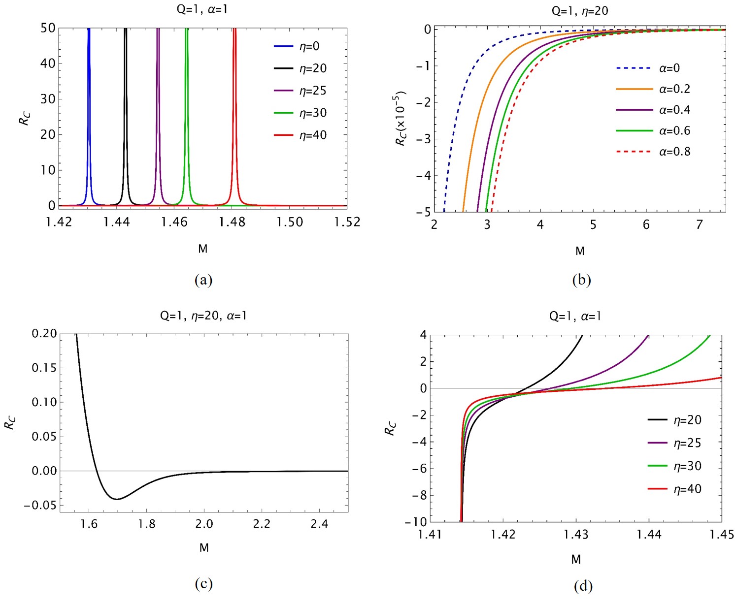
Figure 5: Thermodynamic curvature $R_{C}$ vs black hole size: impact of (a) quantum corrections $\eta$ and (b) Gauss-Bonnet coupling parameter $\alpha$; zoomed-in view of (c) $\eta=20$ plot in (a) and (d) extremal limit $M=\sqrt{Q^{2}+\alpha}.$

In this framework, $R_{C}$ has the following interpretation: a zero curvature indicates that the system is non-interacting and in an ideal gas-like configuration, providing no additional information about black hole micromolecules. A positive $R$ signifies repulsive interactions, indicating an unstable system, while a negative $R$ represents attractive interactions and thus a stable system. Divergences in $R$ correspond to phase transitions Ruppeiner (2014). From this interpretation of $R$, one might wonder if $R$ would be very large for a black hole due to its infinite density. This point is emphasized in Ref. Ruppeiner (2014), where it is suggested that the gravitational degrees of freedom in a black hole system might possess some non-statistical description because all the gravitating material has been compressed into the central singularity. Thus, thermodynamic curvature represents some kind of non-gravitational interactions among the black hole constituents at its surface, arising effectively from the underlying gravitational degrees of freedom.

V Discussion of the Results

Since the expression for thermodynamic curvature $R_{C}$ from Eq. (28) is quite lengthy, we refrain from writing it down here and instead provide a graphical analysis of our results. The results are plotted in Fig. 5 for various choices of the parameters $\eta$ and $\alpha$. A common feature of the plots is immediately evident: $R_{C}=0$ for larger black hole sizes, regardless of the values of $\eta$ and $\alpha$. The deviations from zero begin at smaller scales, where quantum corrections to the entropy become significant. The zero curvature for larger sizes indicates Ruppeiner flatness, suggesting that the black hole resides in a non-interacting phase, akin to an ideal gas. This feature is peculiar to charged black holes in Einstein gravity across all spacetime dimensions Aman et al. (2003); Aman and Pidokrajt (2006); Masood A. S. Bukhari et al. (2023), and interestingly, it is also observed in 4D-EGB theory. For a fixed $Q$ and $\alpha$, $R_{C}$ transitions from zero at larger $M$ values to either positive or negative values for smaller $M$, supplemented with divergences, depending on the values of $\eta$ and $\alpha$. In particular, two divergences exist in $R_{C}$ as shown in Fig. 5(a): one at larger $M$ (positive divergence) and another at the extremal limit of the geometry (negative divergence), occurring at $M=\sqrt{Q^{2}+\alpha}$. Meanwhile, between these two divergences, the black hole also passes through negative $R_{C}$ values [see Fig. 5(c)]. This implies that while the black hole is in an ideal state for larger sizes, it first becomes stable in the quantum regime before attaining instability with positive $R_{C}$.

The positive region for $R_{C}$, accompanied by a positive divergence, indicates two unstable phases for the black hole on either side of the divergent point where a phase transition occurs. The two unstable phases coexist around $R_{C}\rightarrow\infty$ and may generally be different in nature. Each time the magnitude of quantum corrections to the entropy, quantified by $\eta$, increases, the positive divergence in $R_{C}$ shifts to larger $M$, as depicted in Fig. 5(a). However, the second divergence still occurs at the extremal limit for all curves, as evident from Fig. 5(d). As $\alpha$ increases while $Q$ and $\eta$ remain constant [Fig.5(b)], the shifting of the negative divergence of $R_{C}$ occurs along the horizontal axis towards larger $M$, indicating that the black hole stops evaporating earlier than in the previous configuration. This is expected because each time $\alpha$ increases, the term $\sqrt{Q^{2}+\alpha}$ grows, shifting the extremal limit of the black hole geometry to larger sizes.

We also observe from our plots that the black hole remains in the negative $R_{C}$ region as it approaches the extremal limit, indicating that in all situations, the black hole is stable in the quantum regime. The negative divergence of $R_{C}$ at the extremal limit naturally coincides with the zero of the heat capacity at extremal limit [see Fig. 4]. Hence, we may conclude from this coincidence that the Ruppeiner geometry provides a good description of the interacting micromolecules of the black hole.

An interesting observation can be drawn from the above description. The extremal limit is the point where the black hole terminates its evaporation and ends up as a remnant. This occurs when the black hole attains zero temperature, as shown earlier in Fig. 2. Though it is difficult to determine whether the remnant is stable or unstable from this analysis, as the heat capacity $C_{Q}$ and $R_{C}$ become unphysical beyond extremal limit, it is reasonable to make the following observation. In ordinary thermodynamics, as the temperature drops towards absolute zero, the interactions generally freeze out, leaving behind only quantum statistical interactions like those in ideal Fermi or Bose gases Ruppeiner and Sturzu (2023). The extremal limit of the black hole in our case also corresponds to zero temperature, where $R_{C}$ diverges to negative infinity. This may reflect a situation where black hole microstates freeze out, similar to those of an ideal Bose gas, forming a stable remnant.

Although we made efforts to interpret our results based on graphical behavior of computed formulas, it remains worth attempting to to understand the physical mechanisms behind the thermodynamic properties exhibited by black holes on smaller scales. To this end, it is important to note that black hole thermodynamics is perhaps not very well understood, especially at the microscopic level Davies (1978); Page (2005). Adding the complications due to extra curvature corrections from Gauss-Bonnet theory and quantum scale modifications, it becomes increasingly challenging to precisely quantify this thermodynamic behavior. This complexity arises from the combined effects of the parameters involved in the process, as demonstrated in Fig. 5. However, we believe that certain peculiarities regarding $\alpha$ and $\eta$ can still be inferred from these observations. First, note from Eq. 14 (or Eq. 12) that the size dynamics of the black hole are primarily dictated by its mass $M$, which usually dominates over other properties (e.g., charge $Q$). The effect of $\alpha$ on black hole size is thus pronounced only on smaller scales, as it has been tightly constrained Fernandes et al. (2022). We previously highlighted the $Q$-like character of $\alpha$ in that it diminishes the size of the black hole, a situation similar to the Reissner-Nordström geometry in Einstein gravity. This reduction in black hole size has potential implications for its area and surface gravity, which in turn affect its thermodynamic properties such as entropy and temperature. It seems plausible to assume that in such scenarios, the thermodynamic degrees of freedom may be influenced. The Ruppeiner flatness associated with larger black holes might be due to the presence of an equal number of repulsive and attractive interactions. For larger black holes, the extensive area provides equal opportunities for both attractive and repulsive micromolecules to interact. This situation may change at quantum scales, where one type of interaction may dominate, causing the black hole to become selective in its thermodynamic configuration. It appears that the black hole favors attractive micromolecules until it reaches the extremal limit, effectively diminishing the influence of repulsive ones. This may also indicate the emergence of a new kind of interaction at such scales. Given the singular nature of $R_{C}$, there might be connections to quantum gravity, where infinities in physical parameters are prevalent. It is conjectured that a robust quantum geometrothermodynamic approach could either avoid these complications or provide insights to further understand these phenomena.

In passing, it’s worth noting that the conventional understanding of Ruppeiner geometry is rooted in classical gravity and the associated thermodynamic fluctuations in equilibrium configurations. However, on quantum scales, some form of non-equilibrium description for black hole thermodynamics is expected to emerge Pourhassan et al. (2021b, 2022c); Iso and Okazawa (2011); Pourhassan et al. (2021a). Here, we incorporated quantum corrections to the entropy without modifying the geometry of the black hole. This should render the Ruppeiner geometric analysis performed here somewhat effective, as it is based on a quantum-corrected entropy.

VI Conclusion

Four-dimensional Einstein-Gauss-Bonnet (4D-EGB) gravity is a novel theory that extends the Einstein paradigm by incorporating higher-order curvature corrections into gravitational dynamics in four spacetime dimensions. This theory achieves these contributions while circumventing Lovelock’s theorem. In this work, we aimed to evaluate the phenomenological aspects of this novel gravitational theory through a detailed analysis. We conducted a thermodynamic geometric analysis based on the Ruppeiner formalism for a charged black hole, aiming to unveil its thermodynamic phase structure while incorporating non-perturbative quantum corrections to the black hole entropy. Our findings indicate that for large black hole sizes, 4D-EGB exhibits behavior similar to standard general relativity. However, it may signal various types of phase transitions in the quantum regime, contingent upon the Gauss-Bonnet coupling parameter and the magnitude of quantum corrections to the entropy. A striking feature is that our black hole system exhibits a stable regime on quantum scales, where microstates tend to freeze out, resembling a typical Bose gas, as the black hole geometry approaches the extremal limit, coinciding with zero temperature. This scenario may suggest the emergence of a stable remnant, the formation of which is influenced by the strength of the Gauss-Bonnet coupling parameter as it accelerates the coming into being of such remnant.

The analysis can be extended in several ways. Our model is arguably the simplest, considering a charged black hole, which is the most straightforward generalization beyond an uncharged one. Results can be extended to encompass all black hole geometries in the Kerr-Newman family, and later, to include additional matter-energy distributions around the black holes. Considering the intriguing thermodynamic behavior attributed to negative cosmological constant, which are analogized with thermodynamic pressure Kubiznak et al. (2017), extending our formalism to study the corresponding phase structures would be intriguing. This, along with several other ideas, presents possible avenues for future research directions, which will be explored in subsequent studies.

References

- Hawking (1974) S. W. Hawking, Nature 248, 30 (1974).
- Hawking (1975) S. W. Hawking, Commun. Math. Phys. 43, 199 (1975), [Erratum: Commun.Math.Phys. 46, 206 (1976)].
- Bekenstein (1973) J. D. Bekenstein, Phys. Rev. D 7, 2333 (1973).
- Susskind (1995) L. Susskind, J. Math. Phys. 36, 6377 (1995), arXiv:hep-th/9409089 .
- Bousso (2003) R. Bousso, NATO Sci. Ser. II 104, 75 (2003).
- Davies (1978) P. C. W. Davies, Rept. Prog. Phys. 41, 1313 (1978).
- Page (2005) D. N. Page, New J. Phys. 7, 203 (2005), arXiv:hep-th/0409024 .
- Hossenfelder (2013) S. Hossenfelder, Living Rev. Rel. 16, 2 (2013), arXiv:1203.6191 [gr-qc] .
- Mann and Solodukhin (1998) R. B. Mann and S. N. Solodukhin, Nucl. Phys. B 523, 293 (1998), arXiv:hep-th/9709064 .
- Upadhyay et al. (2018) S. Upadhyay, S. H. Hendi, S. Panahiyan, and B. Eslam Panah, PTEP 2018, 093E01 (2018), arXiv:1809.01078 [gr-qc] .
- Pourhassan et al. (2020) B. Pourhassan, S. Dey, S. Chougule, and M. Faizal, Class. Quant. Grav. 37, 135004 (2020), arXiv:1905.03624 [hep-th] .
- Strominger and Vafa (1996) A. Strominger and C. Vafa, Phys. Lett. B 379, 99 (1996), arXiv:hep-th/9601029 .
- Rovelli (1996) C. Rovelli, Phys. Rev. Lett. 77, 3288 (1996), arXiv:gr-qc/9603063 .
- Ashtekar et al. (1998) A. Ashtekar, J. Baez, A. Corichi, and K. Krasnov, Phys. Rev. Lett. 80, 904 (1998).
- Kaul and Majumdar (2000) R. K. Kaul and P. Majumdar, Phys. Rev. Lett. 84, 5255 (2000).
- Dabholkar et al. (2011) A. Dabholkar, J. Gomes, and S. Murthy, JHEP 05, 059 (2011), arXiv:0803.2692 [hep-th] .
- Mandal and Sen (2010) I. Mandal and A. Sen, Class. Quant. Grav. 27, 214003 (2010), arXiv:1008.3801 [hep-th] .
- Ashtekar (1991) A. Ashtekar, Lectures on nonperturbative canonical gravity, Vol. 6 (1991).
- Ghosh and Mitra (2014) A. Ghosh and P. Mitra, Phys. Lett. B 734, 49 (2014), arXiv:1206.3411 [gr-qc] .
- Dabholkar et al. (2015) A. Dabholkar, J. Gomes, and S. Murthy, JHEP 03, 074 (2015), arXiv:1404.0033 [hep-th] .
- Chatterjee and Ghosh (2020) A. Chatterjee and A. Ghosh, Phys. Rev. Lett. 125, 041302 (2020), arXiv:2007.15401 [gr-qc] .
- Maldacena (1998) J. M. Maldacena, Adv. Theor. Math. Phys. 2, 231 (1998), arXiv:hep-th/9711200 .
- Murthy and Pioline (2009) S. Murthy and B. Pioline, JHEP 09, 022 (2009), arXiv:0904.4253 [hep-th] .
- Dabholkar et al. (2013) A. Dabholkar, J. Gomes, and S. Murthy, JHEP 04, 062 (2013), arXiv:1111.1161 [hep-th] .
- Hemming and Thorlacius (2007) S. Hemming and L. Thorlacius, JHEP 11, 086 (2007), arXiv:0709.3738 [hep-th] .
- Gregory et al. (2008) R. Gregory, S. F. Ross, and R. Zegers, JHEP 09, 029 (2008), arXiv:0802.2037 [hep-th] .
- Rocha (2008) J. V. Rocha, JHEP 08, 075 (2008), arXiv:0804.0055 [hep-th] .
- Saraswat and Afshordi (2020) K. Saraswat and N. Afshordi, JHEP 04, 136 (2020), arXiv:1906.02653 [hep-th] .
- Sen (2012) A. Sen, Gen. Rel. Grav. 44, 1947 (2012), arXiv:1109.3706 [hep-th] .
- Govindarajan et al. (2001) T. R. Govindarajan, R. K. Kaul, and V. Suneeta, Class. Quant. Grav. 18, 2877 (2001), arXiv:gr-qc/0104010 .
- Pourhassan et al. (2017) B. Pourhassan, M. Faizal, Z. Zaz, and A. Bhat, Phys. Lett. B 773, 325 (2017), arXiv:1709.09573 [gr-qc] .
- Pourhassan et al. (2018) B. Pourhassan, S. Upadhyay, H. Saadat, and H. Farahani, Nucl. Phys. B 928, 415 (2018), arXiv:1705.03005 [hep-th] .
- Pourhassan et al. (2021a) B. Pourhassan, M. Dehghani, M. Faizal, and S. Dey, Class. Quant. Grav. 38, 105001 (2021a), arXiv:2012.14428 [gr-qc] .
- Upadhyay et al. (2022) S. Upadhyay, N. ul islam, and P. A. Ganai, JHAP 2, 25 (2022), arXiv:1912.00767 [gr-qc] .
- Ghaffarnejad and Ghasemi (2022) H. Ghaffarnejad and E. Ghasemi, JHAP 3, 47 (2022), arXiv:2204.02979 [gr-qc] .
- Biswas et al. (2021) M. Biswas, S. Maity, and U. Debnath, JHAP 1, 71 (2021), arXiv:2110.11770 [gr-qc] .
- Pourhassan et al. (2022a) B. Pourhassan, H. Aounallah, M. Faizal, S. Upadhyay, S. Soroushfar, Y. O. Aitenov, and S. S. Wani, JHEP 05, 030 (2022a), arXiv:2201.11073 [hep-th] .
- Pourhassan et al. (2022b) B. Pourhassan, M. Atashi, H. Aounallah, S. S. Wani, M. Faizal, and B. Majumder, Nucl. Phys. B 980, 115842 (2022b), arXiv:2205.13584 [gr-qc] .
- Aounallah et al. (2022) H. Aounallah, H. El Moumni, J. Khalloufi, and K. Masmar, Int. J. Mod. Phys. A 37, 2250036 (2022).
- Masood A. S. Bukhari et al. (2023) S. Masood A. S. Bukhari, B. Pourhassan, H. Aounallah, and L.-G. Wang, Class. Quant. Grav. 40, 225007 (2023), arXiv:2304.00940 [gr-qc] .
- Iso and Okazawa (2011) S. Iso and S. Okazawa, Nucl. Phys. B 851, 380 (2011), arXiv:1104.2461 [hep-th] .
- Abbott et al. (2016a) B. P. Abbott et al. (LIGO Scientific, Virgo), Phys. Rev. Lett. 116, 061102 (2016a), arXiv:1602.03837 [gr-qc] .
- Abbott et al. (2016b) B. P. Abbott et al. (LIGO Scientific, Virgo), Phys. Rev. Lett. 116, 221101 (2016b), [Erratum: Phys.Rev.Lett. 121, 129902 (2018)], arXiv:1602.03841 [gr-qc] .
- Akiyama et al. (2019) K. Akiyama et al. (Event Horizon Telescope), Astrophys. J. Lett. 875, L1 (2019), arXiv:1906.11238 [astro-ph.GA] .
- Capozziello and De Laurentis (2011) S. Capozziello and M. De Laurentis, Phys. Rept. 509, 167 (2011), arXiv:1108.6266 [gr-qc] .
- Berti et al. (2015) E. Berti et al., Class. Quant. Grav. 32, 243001 (2015), arXiv:1501.07274 [gr-qc] .
- Shankaranarayanan and Johnson (2022) S. Shankaranarayanan and J. P. Johnson, Gen. Rel. Grav. 54, 44 (2022), arXiv:2204.06533 [gr-qc] .
- Lanczos (1938) C. Lanczos, Annals Math. 39, 842 (1938).
- Lovelock (1971) D. Lovelock, J. Math. Phys. 12, 498 (1971).
- Lovelock (1972) D. Lovelock, J. Math. Phys. 13, 874 (1972).
- Blázquez-Salcedo et al. (2016) J. L. Blázquez-Salcedo, C. F. B. Macedo, V. Cardoso, V. Ferrari, L. Gualtieri, F. S. Khoo, J. Kunz, and P. Pani, Phys. Rev. D 94, 104024 (2016), arXiv:1609.01286 [gr-qc] .
- Konoplya et al. (2020) R. A. Konoplya, T. Pappas, and A. Zhidenko, Phys. Rev. D 101, 044054 (2020), arXiv:1907.10112 [gr-qc] .
- Maselli et al. (2015) A. Maselli, L. Gualtieri, P. Pani, L. Stella, and V. Ferrari, Astrophys. J. 801, 115 (2015), arXiv:1412.3473 [astro-ph.HE] .
- Ayzenberg et al. (2014) D. Ayzenberg, K. Yagi, and N. Yunes, Phys. Rev. D 89, 044023 (2014), arXiv:1310.6392 [gr-qc] .
- Ostrogradsky (1850) M. Ostrogradsky, Mem. Acad. St. Petersbourg 6, 385 (1850).
- Zwiebach (1985) B. Zwiebach, Phys. Lett. B 156, 315 (1985).
- Gross and Witten (1986) D. J. Gross and E. Witten, Nucl. Phys. B 277, 1 (1986).
- Gross and Sloan (1987) D. J. Gross and J. H. Sloan, Nucl. Phys. B 291, 41 (1987).
- Glavan and Lin (2020) D. Glavan and C. Lin, Phys. Rev. Lett. 124, 081301 (2020), arXiv:1905.03601 [gr-qc] .
- Lu and Pang (2020) H. Lu and Y. Pang, Phys. Lett. B 809, 135717 (2020), arXiv:2003.11552 [gr-qc] .
- Hennigar et al. (2020) R. A. Hennigar, D. Kubizňák, R. B. Mann, and C. Pollack, JHEP 07, 027 (2020), arXiv:2004.09472 [gr-qc] .
- Gürses et al. (2020) M. Gürses, T. c. Şişman, and B. Tekin, Eur. Phys. J. C 80, 647 (2020), arXiv:2004.03390 [gr-qc] .
- Konoplya and Zinhailo (2020) R. A. Konoplya and A. F. Zinhailo, Eur. Phys. J. C 80, 1049 (2020), arXiv:2003.01188 [gr-qc] .
- Kumar and Ghosh (2020) R. Kumar and S. G. Ghosh, JCAP 07, 053 (2020), arXiv:2003.08927 [gr-qc] .
- Guo and Li (2020) M. Guo and P.-C. Li, Eur. Phys. J. C 80, 588 (2020), arXiv:2003.02523 [gr-qc] .
- Wei and Liu (2020) S.-W. Wei and Y.-X. Liu, Phys. Rev. D 101, 104018 (2020), arXiv:2003.14275 [gr-qc] .
- Hosseini Mansoori (2021) S. A. Hosseini Mansoori, Phys. Dark Univ. 31, 100776 (2021), arXiv:2003.13382 [gr-qc] .
- Eslam Panah et al. (2020) B. Eslam Panah, K. Jafarzade, and S. H. Hendi, Nucl. Phys. B 961, 115269 (2020), arXiv:2004.04058 [hep-th] .
- Fernandes et al. (2022) P. G. S. Fernandes, P. Carrilho, T. Clifton, and D. J. Mulryne, Class. Quant. Grav. 39, 063001 (2022), arXiv:2202.13908 [gr-qc] .
- Ruppeiner (2014) G. Ruppeiner, Springer Proc. Phys. 153, 179 (2014), arXiv:1309.0901 [gr-qc] .
- Fernandes (2020) P. G. S. Fernandes, Phys. Lett. B 805, 135468 (2020), arXiv:2003.05491 [gr-qc] .
- Jacobson (1995) T. Jacobson, Phys. Rev. Lett. 75, 1260 (1995).
- Faizal et al. (2017) M. Faizal, A. Ashour, M. Alcheikh, L. Alasfar, S. Alsaleh, and A. Mahroussah, Eur. Phys. J. C 77, 608 (2017), arXiv:1710.06918 [gr-qc] .
- Penrose (1969) R. Penrose, Riv. Nuovo Cim. 1, 252 (1969).
- Hiscock and Weems (1990) W. A. Hiscock and L. D. Weems, Phys. Rev. D 41, 1142 (1990).
- Hendi and Momennia (2018) S. H. Hendi and M. Momennia, Phys. Lett. B 777, 222 (2018).
- Ruppeiner (1995) G. Ruppeiner, Rev. Mod. Phys. 67, 605 (1995), [Erratum: Rev.Mod.Phys. 68, 313–313 (1996)].
- Weinhold (1975a) F. Weinhold, The Journal of Chemical Physics 63, 2479 (1975a), https://doi.org/10.1063/1.431689 .
- Weinhold (1975b) F. Weinhold, The Journal of Chemical Physics 63, 2484 (1975b), https://doi.org/10.1063/1.431635 .
- Ruppeiner (1979) G. Ruppeiner, Phys. Rev. A 20, 1608 (1979).
- Ruppeiner (1981) G. Ruppeiner, Phys. Rev. A 24, 488 (1981).
- Janyszek and Mrugala (1989) H. Janyszek and R. Mrugala, Phys. Rev. A 39, 6515 (1989).
- Quevedo (2007) H. Quevedo, J. Math. Phys. 48, 013506 (2007), arXiv:physics/0604164 .
- Quevedo and Sanchez (2008) H. Quevedo and A. Sanchez, JHEP 09, 034 (2008), arXiv:0805.3003 [hep-th] .
- Hendi et al. (2015) S. H. Hendi, S. Panahiyan, B. Eslam Panah, and M. Momennia, Eur. Phys. J. C 75, 507 (2015), arXiv:1506.08092 [gr-qc] .
- Carroll (2019) S. M. Carroll, Spacetime and Geometry (Cambridge University Press, 2019).
- Aman et al. (2003) J. E. Aman, I. Bengtsson, and N. Pidokrajt, Gen. Rel. Grav. 35, 1733 (2003), arXiv:gr-qc/0304015 .
- Aman and Pidokrajt (2006) J. E. Aman and N. Pidokrajt, Phys. Rev. D 73, 024017 (2006), arXiv:hep-th/0510139 .
- Ruppeiner and Sturzu (2023) G. Ruppeiner and A.-M. Sturzu, Phys. Rev. D 108, 086004 (2023), arXiv:2304.06187 [gr-qc] .
- Pourhassan et al. (2021b) B. Pourhassan, S. S. Wani, S. Soroushfar, and M. Faizal, JHEP 10, 027 (2021b), arXiv:2102.03296 [hep-th] .
- Pourhassan et al. (2022c) B. Pourhassan, I. Sakalli, X. Shi, M. Faizal, and S. S. Wani, (2022c), arXiv:2301.00687 [hep-th] .
- Kubiznak et al. (2017) D. Kubiznak, R. B. Mann, and M. Teo, Class. Quant. Grav. 34, 063001 (2017), arXiv:1608.06147 [hep-th] .