Majorana Zero Modes in Lieb-Kitaev Model with Tunable Quantum Metric

Abstract

The relation between band topology and Majorana zero energy modes (MZMs) in topological superconductors had been well studied in the past decades. However, the relation between the quantum metric and MZMs has yet to be understood. In this work, we first introduce a three band Lieb-like lattice model with an isolated flat band and tunable quantum metric. By introducing nearest neighbor equal spin pairing, we obtain the Lieb-Kitaev model which supports MZMs. When the Fermi energy is set within the flat band, the MZMs are supposed to be well-localized at the ends of the 1D superconductor due to the flatness of the band. On the contrary, we show both numerically and analytically that the localization length of the MZMs is controlled by a length scale defined by the quantum metric of the flat band, which we call the quantum metric length (QML). The QML can be several orders of magnitude longer than the conventional BCS superconducting coherence length. When the QML is comparable to the length of the superconductor, the two MZMs from the two ends of the superconductor can hybridize. When two metallic leads are coupled to the two MZMs, crossed Andreev reflection probability can nearly reach the maximal theoretical value. This work unveils how the quantum metric can greatly influence the properties of MZMs through the QML and the results can be generalized to other topological bound states.

Introduction.— Majorana zero energy modes (MZMs) are non-Abelian excitations in topological superconductors Read and Green (2000); Kitaev (2001); Ivanov (2001); Stone and Chung (2006); Fu and Kane (2008); Fujimoto (2008); Nilsson et al. (2008); Fu and Kane (2009a, b); Akhmerov et al. (2009); Sato et al. (2009); Law et al. (2009); Sau et al. (2010); Alicea (2010); Lutchyn et al. (2010); Oreg et al. (2010); Flensberg (2010); Potter and Lee (2010); Alicea et al. (2010); Cook and Franz (2011); He et al. (2014), which have potential applications in fault-tolerant quantum computation Kitaev (2003); Nayak et al. (2008); Aasen et al. (2016). Due to the non-Abelian nature of MZMs and their ability to store quantum information which are immune to local perturbations, the study of MZMs has been one of the most important topics in condensed matter physics in the past few decades Hasan and Kane (2010); Qi and Zhang (2011); Alicea (2012); Beenakker (2013). As first pointed out by Read and Green Read and Green (2000), two-dimensional $p+ip$ superconductors which are characterized by nontrivial Chern numbers support chiral Majorana edge modes. The Chern number is defined as the sum of the Berry curvature of occupied quasiparticle states of the Bogoliubov-de Gennes (BdG) Hamiltonian. Using a single band model with spinless $p$-wave pairing (Fig. 1(a)), Kitaev pointed out that one-dimensional topological superconductors support MZMs which are localized at the two ends of the superconducting wires Kitaev (2001).

After the above seminal works Read and Green (2000); Kitaev (2001), a large number of studies had contributed to the experimental realization and detection of MZMs Mourik et al. (2012); Rokhinson et al. (2012); Das et al. (2012); Deng et al. (2012); Nadj-Perge et al. (2014); Albrecht et al. (2016); Jäck et al. (2019); Fornieri et al. (2019); Ren et al. (2019); Wang et al. (2018). However, previous works were mostly focused on the topological aspects of MZMs, which are essentially connected to the Berry curvatures of the quasiparticle states. Interestingly, the Berry curvature is only one of the two aspects of the so-called quantum geometry of the quantum states Provost and Vallee (1980); Berry (1984); Resta (2010). Given a Bloch state labeled by crystal momentum $\bm{k}$, we can construct the quantum geometry tensor $\mathfrak{G}(\bm{k})=\mathcal{G}(\bm{k})-i\mathcal{F}(\bm{k})/2$ Resta (2010). Here, the real part $\mathcal{G}$ is the quantum metric of the Bloch states and the imaginary part $\mathcal{F}$ is the Berry curvature . The study of quantum metric effects has attracted much attention in recent years Haldane (2011); Parameswaran et al. (2013); Neupert et al. (2013); Gao et al. (2014); Roy (2014); Peotta and Törmä (2015); Julku et al. (2016); Liang et al. (2017); Iskin (2018); Hofmann et al. (2020); Verma et al. (2021); Kozii et al. (2021); Ahn and Nagaosa (2021); Julku et al. (2021); Chen and Huang (2021); Herzog-Arbeitman et al. (2022); Ahn et al. (2022); Hofmann et al. (2023); Chen and Law (2024); Kitamura et al. (2024). While the effect of Berry curvature on the topological superconductors had been intensively studied in the past decades, the relation between the quantum metric and the properties of the topological bound states has yet to be understood. This work is devoted to understanding the connection between the quantum metric and the properties of the MZMs.

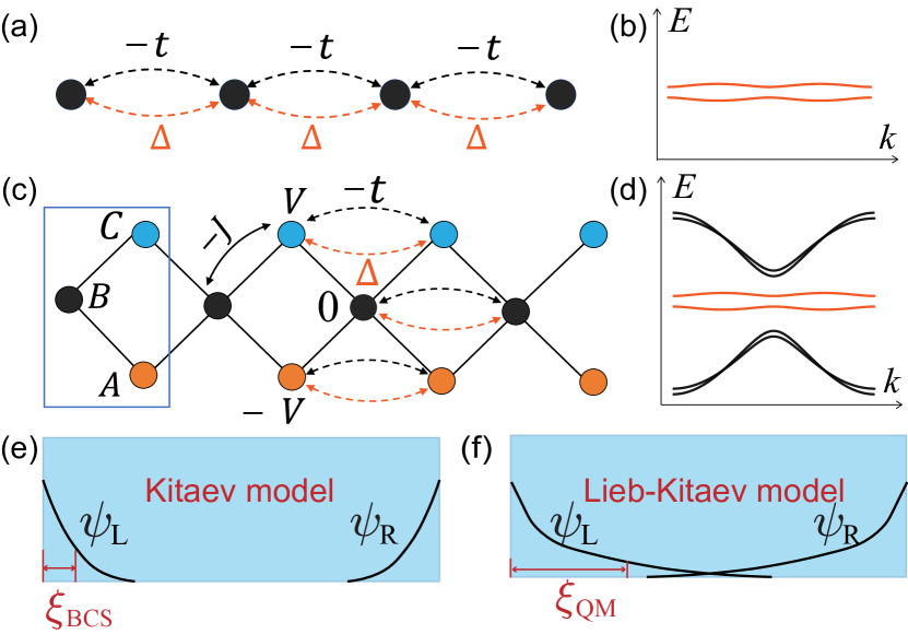
Figure 1: (a) and (c): Schematic illustrations of the real space single band Kitaev model (a) and the three band Lieb-Kitaev model (c). In (a), $t$ denotes the nearest neighbor hopping and $\Delta$ is the nearest neighbor pairing. In (c): Each unit cell contains three lattice sites $A$,$B$ and $C$, respectively. $J$, $t$ and $\Delta$ are the nearest neighbor hopping, the next nearest neighbor hopping, and the nearest neighbor pairing, respectively. (b) and (d): Illustrations of the band structure of the Kitaev model (b) and the Lieb-Kitaev model (d). (e) and (f): Illustrations of the Majorana wavefunctions $\psi_{\text{L}}$ and $\psi_{\text{R}}$ of the Kitaev model (e) and the Lieb-Kitaev model (f). The spread of $\psi_{\text{L/R}}$ is controlled by $\xi_{\text{BCS}}\approx at/\Delta$ in the Kitaev model, and by the QML $\xi_{\text{QM}}$ in the Lieb-Kitaev model, respectively.

To study the quantum metric effects on MZMs, we introduce the Lieb-Kitaev model which supports MZMs and with tunable quantum metric. In the normal state, the model is a spinless Lieb-like lattice which has three orbitals per unit cell (Fig. 1(c)) and this results in a (nearly) flat band between two dispersive bands in the energy spectrum (Fig. 2(a)). In this work, to demonstrate the importance of quantum metric effects, we focus on the regime where the Fermi energy lies within the flat band. Subsequently, we add nearest neighbor intra-orbital pairings to the Lieb-like lattice to create a $p$-wave superconductor which supports MZMs. The resulting Bogoliubov quasiparticle bands are schematically illustrated in Fig. 1(d). The Majorana wavefunctions are illustrated in Fig. 1(f).

There are three important results in this work. First, the quantum metric, which measures the quantum distance between two states Provost and Vallee (1980); Resta (2010), can set a length scale which we call the quantum metric length (QML) $\xi_{\text{QM}}$ as defined in Eq. (3) Chen and Law (2024); Hu et al. (2024). The QML, defined as the average of the quantum metric over the Brillouin zone, governs the localization length as well as the quadratic spread of the Majorana wavefunctions for superconductors with (nearly) flat bands. Importantly, the QML is tunable and it can be several orders of magnitude longer than the lattice length scale as illustrated in Fig. 2(b). Second, in flat band topological superconductors with long QML, the two MZMs from the two ends of the topological superconductor can hybridize with each other over a long distance even though the conventional BCS superconducting coherence length $\xi_{\text{BCS}}$ of the flat band superconductor is short. Here, $\xi_{\text{BCS}}\approx at/\Delta$ where $2t$ is the bandwidth, $\Delta$ is the pairing amplitude of the flat band and $a$ is the lattice constant. Third, the hybridization of MZMs can result in long range nonlocal transport processes such as crossed Andreev reflections (CARs) when two metallic leads are connected to the two MZMs separately Law et al. (2009); Nilsson et al. (2008); Liu et al. (2013). Remarkably, the CAR amplitudes can be comparable to the maximal theoretical value even when the separation of leads is several orders of magnitude longer than the $\xi_{\text{BCS}}$ of the flat band.

Lieb-Kitaev model.— In this section, we introduce the Lieb-Kitaev model for the realization of topological superconductors with tunable quantum metric. In the normal state of the Lieb-like lattice, the on-site energies of the $(A,B,C)$ orbitals are $(-V,0,V)$ respectively, as illustrated in Fig. 1(c). The nearest neighbor hopping amplitude is $J$. Additionally, a much smaller intra-orbital hopping $t$ is introduced (black dashed lines in Fig. 1(c)). Accordingly, the Hamiltonian in the Bloch basis $\hat{\bm{c}}(k)=\left(\hat{c}_{A}(k),\hat{c}_{B}(k),\hat{c}_{C}(k)\right)^{\text{T}}$ is written as

$$h(k)=(-2t\cos{(ka)}-\mu)\mathbb{I}_{3}+\begin{pmatrix}-V&a_{k}&0\\ a_{k}^{*}&0&a_{k}^{*}\\ 0&a_{k}&V\end{pmatrix}.$$ (1)

Here, $\mu$ is the chemical potential, $a_{k}=-J(1+e^{ika})$ where $a$ is the lattice constant, and $\mathbb{I}_{3}$ is the identity matrix. Fig. 2(a) depicts the band structure of the model as defined in Eq. (1). We focus on the (nearly) flat band with dispersion $\epsilon_{0}=-2t\cos{(ka)}-\mu$, where $2t$ is the bandwidth of the flat band. When $t=0$, the band is exactly flat (blue line in Fig 2(a)). The flat band is separated from two dispersive bands by an energy gap $E_{\text{g}}=|V|$. The eigenstates of the flat band are

$$u_{0}(k)=(a_{k},V,-a_{k})^{T}/\sqrt{4J^{2}(1+\cos{(ka)})+V^{2}},$$ (2)

which is essential for computing the quantum metric as well as constructing the Majorana wavefunctions as shown below.

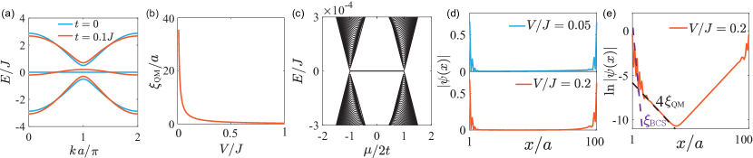
Figure 2: (a) The normal state energy spectrum with $t=0$ (blue line) and $t=0.1J$ (orange line), respectively. $J=1$ and $V=0.2J$ are assumed in Eq. (1). (b) QML as a function of $V/J$. (c) Energy levels of a lattice model of $H_{\text{BDG}}$ as a function of $\mu/2t$ with open boundary conditions. The parameters are $\mu=0$, $t=3\times 10^{-4}J$, $\Delta=0.6t$ and $V=0.2J$. The zero energy modes appear in the topological regime $|\mu|<2t$. (d) The wavefunction amplitudes of MZMs with different $V/J$. The length of the superconductor $L=100a$. The parameters are the same as in (c) except $V/J$. (e) $\ln{|\psi(x)|}$ is plotted for $|\psi(x)|$ in (d) with $V/J=0.2$. The short distance localization length is controlled by $\xi_{\text{BCS}}$ (dotted purple line) and the long distance localization length (dotted black line) is controlled by $4\xi_{\text{QM}}$. The numerical results are in perfect agreement with Eq. (7).

The quantum metric of a state with momentum $k$ of the flat band is defined as $\mathcal{G}(k)=\bra{\partial_{k}u_{0}(k)}\left[\mathbb{I}-\ket{u_{0}(k)}\bra{u_{0}(k)}\right]\ket{\partial_{k}u_{0}(k)}$ which has the dimension of length-squared. The QML $\xi_{\text{QM}}$ is defined as the Brillouin zone averaged quantum metric:

$$\xi_{\text{QM}}\equiv\int_{0}^{2\pi/a}\mathcal{G}(k)\frac{dk}{2\pi}\overset{\frac{V}{J}\rightarrow 0}{\longrightarrow}\frac{\sqrt{2}}{4}\frac{J}{V}a.$$ (3)

The length scale $\xi_{\text{QM}}$ is particularly important for exactly flat bands with $t=0$ and vanishing Fermi velocity. In this case, the conventional length scales such as the Fermi wavelength is not well-defined and the BCS coherence length $\xi_{\text{BCS}}\approx at/\Delta$ is zero for flat bands. As we show below, the QML $\xi_{\text{QM}}$ is still a dominant length scale which governs the spread of the Majorana wavefunctions in topological superconductors when $\xi_{\text{QM}}$ is longer than $\xi_{\text{BCS}}$. Moreover, for the Lieb-like lattice, the $\xi_{\text{QM}}$ is tunable by changing $V/J$. Fig. 2(b) shows that $\xi_{\text{QM}}$ is divergent when $V/J$ approaches $0$. With the tunable QML, the Lieb-like lattice is an ideal model for studying the interplay between the topology and quantum metric.

To realize MZMs, we introduce intra-orbital pairing with amplitude $\Delta$ between sites from adjacent unit cells, indicated by the red dashed line in Fig. 1(c). The resulting BdG Hamiltonian of the Lieb-Kitaev model is

$$H_{\text{BdG}}=\sum_{k}\hat{\Psi}^{\dagger}(k)\begin{pmatrix}h(k)&-i2\Delta\sin{(ka)}\mathbb{I}_{3}\\ i2\Delta\sin{(ka)}\mathbb{I}_{3}&-h^{*}(-k)\end{pmatrix}\hat{\Psi}(k),$$ (4)

where $\hat{\Psi}(k)=(\hat{\bm{c}}(k),\hat{\bm{c}}^{\dagger}(-k))^{\text{T}}$. Fig. 2(c) shows the energy levels of a finite size system with open boundary conditions within the energy window $E\in[-t,t]$. We observe that zero energy modes exist when the chemical potential lies in the region $|\mu|<2t$. The topological phase is characterized by the Z2 number $Q=\operatorname{sign}(\text{Pf}[i\tilde{H}(k=0)]\text{Pf}[i\tilde{H}(k=\frac{\pi}{a})]$ Kitaev (2001); Schnyder et al. (2008). As shown in the Supplemental Material Not , in cases of $|\mu|<2t$, we have $\mathcal{Q}=-1$, which corresponds to the topologically nontrivial regime.

Fig. 2(d) depicts the Majorana wavefunctions of the models with two different values of $V/J$ and $\Delta=0.6t$ such that the band is extremely flat. With a larger quantum metric (smaller $V/J$), the Majorana wavefunctions can penetrate deeper into the bulk of the flat band superconductor. The localization length of the Majorana wavefunctions is indeed much longer than $t/\Delta$ which is different from the single band Kitaev model. The asymmetry of the Majorana wavefunctions from the two ends of the superconductor originates from the inversion symmetry breaking of the underlying lattice. To quantify the spread of the Majorana wavefunctions, we plot $\ln{|\psi(x)|}$ versus position $x$ in Fig. 2(e). Here, $\psi(x)$ is the wavefunction of the fermionic mode which includes the Majorana wavefunctions from the left and the right boundaries. For the Majorana modes of the left boundary, for example, there are two different decay modes in short and long distances as shown in Fig. 2(e). At a relative short distance away from the left boundary, the Majorana wavefunction decays as $e^{-x/\xi_{\text{BCS}}}$ (purple dashed line in Fig. 2(e)), where $\xi_{\text{BCS}}=-2a/\ln{\left(\frac{t-\Delta}{t+\Delta}\right)}$ Leumer et al. (2020). For $t\gg\Delta$, we have $\xi_{\text{BCS}}\approx at/\Delta$ and we call this length the BCS coherence length. However, at larger $x$, a different decay behavior takes over and the wavefunction decays as $e^{-x/4\xi_{\text{QM}}}$ (black dashed line in Fig. 2(e)), where $\xi_{\text{QM}}$ is the QML defined in Eq. (3). In the next section, we will show analytically how the QML emerges in the Majorana wavefunctions.

Wavefunctions, localization length and quadratic spread of MZMs.— To begin with, we consider the multiband Hamiltonian $H=H_{0}+H_{1}$, where $H_{0}$ is the lattice representation of Eq. (4) with $N$ sites and a periodic boundary condition. The perturbation $H_{1}$ removes the hopping and pairing between the first site $1$ and the last site $N$ of $H_{0}$ and the addition of $H_{1}$ results in a Hamiltonian with an open boundary condition Mong and Shivamoggi (2011). For $V\gg t\simeq\Delta$ and $|\mu|<2t$, the two isolated quasi-particle bands labeled by $n=\pm$ respectively are close to the Fermi energy and far away from other bands. The eigenstates of the $n=\pm$ bands are denoted by $g_{n}(k)$ where $H_{\text{BdG}}(k)g_{n}(k)=\varepsilon_{n}(k)g_{n}(k)$. The eigenstate $\psi(x)$ which contains the two Majorana wavefunctions can be expressed in a self-consistent way as:

$$\psi(x)=-G^{p}(x,Na;E)U_{01}\psi(a)-G^{p}(x,a;E)U_{01}^{\dagger}\psi(Na),$$ (5)

where

$$G^{p}(x_{j},x_{j^{\prime}};E)=\frac{1}{N}\sum_{n=\pm}\sum_{k}\frac{g_{n}(k)g^{\dagger}_{n}(k)}{E-\varepsilon_{n}(k)}e^{ik(x_{j}-x_{j^{\prime}})}$$ (6)

is defined by the projected Green function where $j/j^{\prime}$ is the site index and $E=0$ for the MZMs. The operator $U_{01}$ defines $H_{1}$. The details of the calculations for the Majorana wavefunctions are presented in the Supplemental Material Not .

Away from the left boundary (the first site) and by setting $\mu=0$ for simplicity, the Majorana wavefunction can be written as

$$\psi_{\text{L}}(x_{j})=A_{\text{L}}^{\text{QM}}e^{-\frac{(j-1)a}{4\xi_{\text{QM}}}}+A_{\text{L}}^{\text{BCS}}e^{-\frac{(j-1)a}{\xi_{\text{BCS}}}}.$$ (7)

Here, $A_{\text{L}}^{\text{QM}}$ and $A_{\text{L}}^{\text{BCS}}$ are the amplitudes of two parts of the wavefunction with different localization lengths $4\xi_{\text{QM}}$ and $\xi_{\text{BCS}}$ respectively. The localization lengths are determined by the poles of $g_{n}(k)g^{\dagger}_{n}(k)/\varepsilon_{n}(k)$ in the complex plane. Physically, $\xi_{\text{BCS}}=-2a/\ln{\left(\frac{t-\Delta}{t+\Delta}\right)}$ originates from the dispersion of quasi-particle bands $\varepsilon_{\pm}(k)$. This decay length is the same as the one in the single band Kitaev model with bandwidth $2t$ and pairing potential $\Delta$ Leumer et al. (2020). Importantly, an extra pole of the Bloch wavefunctions gives rise to a decay length of $4\xi_{\text{QM}}$ for the $A_{\text{L}}^{\text{QM}}$ component of the wavefunction. When $4\xi_{\text{QM}}\gg\xi_{\text{BCS}}$, the QML $\xi_{\text{QM}}$ dominates the long range behavior of the Majorana wavefunction. The $A_{\text{L}}^{\text{BCS}}$ component has different amplitudes for the even or odd lattice sites, which explains the oscillation of MZMs’ wavefunction. A similar expression for the wavefunction localized near the right boundary (the Nth-site) $\psi_{\text{R}}(x_{j})$ is shown the Supplemental Material Not . To compare the analytical results with the numerical results, the long distance localization length of MZMs $\xi$ is extracted numerically (orange squared line) and it matches the analytical values of $4\xi_{\text{QM}}$ (blue stared line) perfectly, as shown in Fig. 3(a).

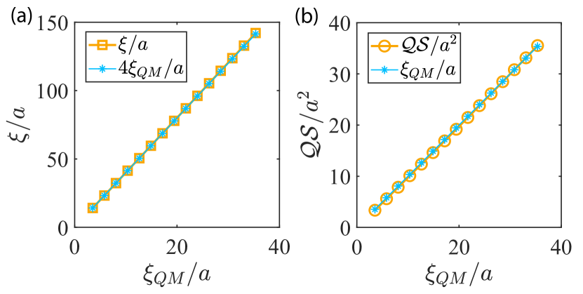
Figure 3: (a) A comparison between the localization length of a MZM extracted numerically $\xi$, and $4\xi_{\text{QM}}$. (b) The quadratic spread $\mathcal{QS}$ of MZMs as a function of QML $\xi_{\text{QM}}$. The results are in agreement with Eq. (8). The parameters of the lattice model for both figures are $\mu=0$, $t=5\times 10^{-4}J$, $\Delta=4.95\times 10^{-4}J$ and $V/J\in[0.01,0.1]$.

Besides the localization length, the spread of a wavefunction can also be characterized by the quadratic spread which was used to measure the size of Wannier states Marzari and Vanderbilt (1997). The quadratic spread of the Majorana wavefunctions can be evaluated as $\mathcal{QS}=\mathcal{QS}_{\text{L}}+\mathcal{QS}_{\text{R}}=\int(x-x_{\text{L}})^{2}|\psi_{\text{L}}(x)|^{2}dx+\int(x-x_{\text{R}})^{2}|\psi_{\text{R}}(x)|^{2}dx$, and $x_{\text{L(R)}}$ is the position of the left (right) boundary. In the limit of small $V/J$, $t\approx\Delta$ and $\mu=0$, to order $\mathcal{O}(V/J)$, we have

$$\mathcal{QS}=\frac{a}{2\pi}\int_{0}^{2\pi/a}\mathcal{G}(k)dk=a\xi_{\text{QM}}.$$ (8)

The analytical results are also in agreement with the numerical results as shown in Fig. 3(b). This is one of the key result of this work as it connects the quantum metric with the spread of the Majorana wavefunctions. The details of the derivation for Eq. (8) are given in the Supplemental Material Not .

Long range crossed Andreev reflection.— In this section, we show that a long quantum metric length can induce long range nonlocal transport when two leads are coupled to the two MZMs separately. In particular, the CAR probability can nearly reach the maximal theoretical value even though the separation of the two leads is several orders of magnitude longer than the conventional localization length of the Majorana modes $\xi_{\text{BCS}}$ in the one band Kitaev model.

Considering a device shown in Fig. 4(a), two normal metal leads are attached to two sides of the topological superconductor. A CAR process happens when an incoming electron from one lead is reflected as a hole in the other lead, leading to the formation of a Cooper pair in the grounded superconductor Law et al. (2009); Nilsson et al. (2008); Liu et al. (2013). Due to the quantum metric induced spread of the Majorana modes as discussed above, the coupling between Majorana modes can be significant in a long topological superconducting wire. We expect that the coupled Majorana modes can mediate long range CARs as shown below.

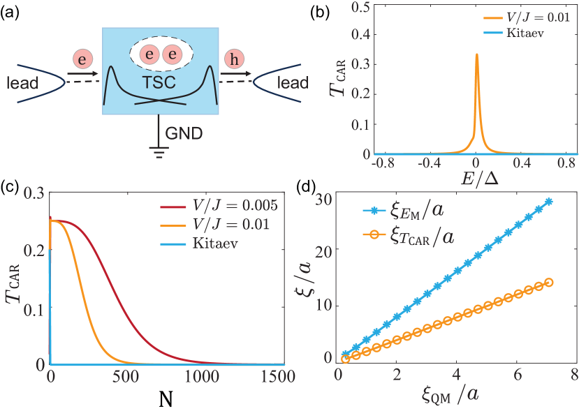
Figure 4: (a) A schematic plot of a normal lead/topological superconductor (TSC)/normal lead device. Two leads couple to the two MZMs separately. In a CAR process, an electron from the left lead is reflected as a hole in the other lead. (b) The CAR probability versus bias voltage $E=eV$ for the single band Kitaev model (blue line) and the Lieb-Kitaev model (yellow line). Parameters $J=1$, $t=1\times 10^{-4}J$, $\Delta=0.8t$, $\mu=0.2t$ and $L=100a$. $V/J=0.01$ is set for Lieb-Kitaev model. The same $\mu$, $t$ and $\Delta$ are set for the single band Kitaev model. (c) The CAR probability at zero bias $E=0$ versus device length $L=Na$ for the Kitaev model (blue line) and the Lieb-Kitaev model with $V/J=0.005$ (red line) and $V/J=0.01$ (yellow line), respectively. (d) The long distance behavior of the hybridization energy $E_{\text{M}}$ of the MZMs and the CAR probability $T_{\text{CAR}}$ as a function of the length of the superconductor can be written as $E_{\text{M}}\propto e^{-Na/\xi_{E_{\text{M}}}}$ and $T_{\text{CAR}}\propto e^{-Na/\xi_{T_{\text{CAR}}}}$. Here, we show that $\xi_{E_{\text{M}}}=4\xi_{\text{QM}}$ and $\xi_{T_{\text{CAR}}}=2\xi_{\text{QM}}$. The parameters in (c) and (d) are the same as in (b) except $L$.

To be more specific, we perform recursive Green function calculations Datta (1995) to study the CAR probability $T_{\text{CAR}}$ for both the single band Kitaev model and the Lieb-Kitaev model. The blue line in Fig. 4(c) shows that the CAR signal only survives in a short wire with a few tens of lattice sites for the single band Kitaev model (Fig. 1(a)). The $T_{\text{CAR}}$ diminishes quickly once the length of the superconductor increases as the MZMs cannot couple to each other due to the short localization lengths of the MZMs in the single band Kitaev model $\xi_{\text{BCS}}$.

In sharp contrast, as indicated by the red and yellow lines in Fig. 4(b)-(c), the CAR probability is significantly enhanced in the Lieb-Kitaev model with large quantum metric. The $T_{\text{CAR}}$ is most significant at low bias, as shown in Fig. 4(b). When the energy of the incoming electron is close to the energy of the fermionic mode formed by the hybrization of the MZMs, a large CAR probability, which is near the maximal theoretical value of 0.5, is possible Nilsson et al. (2008) . Fig. 4(c) depicts $T_{\text{CAR}}$ versus the length of the superconductor at zero bias (red and yellow lines). We find that $T_{\text{CAR}}$ can be large when the separation of the leads is comparable to the QML even when the QML is several orders of magnitude longer than $at/\Delta$. It is striking that the CAR amplitude remains finite up to thousands of sites in cases of larger QML (red line in Fig. 4(c)) when $t/\Delta\approx 1$.

A more careful analysis shows that at low voltage bias, the CAR probability is closely related to the coupling between the two MZMs. The strength of coupling between the MZMs is characterized by the hydridization energy $E_{\text{M}}$. As shown in Fig. 4(d), we found that the hydridization energy is proportional to the length of the topological superconductor such that $E_{\text{M}}\propto e^{-Na/4\xi_{\text{QM}}}$. Accordingly, the CAR probability can be expressed as $T_{\text{CAR}}\propto e^{-Na/2\xi_{\text{QM}}}$ (yellow line in Fig. 4(d)).

Discussion.— In this work, we construct the Lieb-Kitaev model to study the effect of quantum metric on MZMs. It is shown that the localization length as well as the quadratic spread of the Majorana wavefunctions are controlled by the QML in a flat band topological superconductor. Importantly, the Majorana wavefunctions can spread far away from the boundaries when the QML is long. The two MZMs can couple to each other when the QML is comparable to the length of the flat band topological superconductor. The coupling of MZMs can induce long range CARs when two leads are coupled to the two ends of the topological superconductors. It is important to note that the Lieb-Kitaev model proposed only involves the nearest neighbor hopping and pairing. Therefore, quasi-one-dimensional moiré materials, which can be described by Lieb-like lattice Po et al. (2019) in the normal state, can possibly be used to realize the Lieb-Kitaev model. Importantly, the QML is defined by the wavefunctions of the normal state. Therefore, the conclusions of this work can be generalized to describe topological bound states in other topological materials.

Acknowledgements.— We thank Shuai Chen, Adrian Po and Bohm-Jung Yang for inspiring discussions. K. T. L. acknowledges the support of the Ministry of Science and Technology, China, and Hong Kong Research Grant Council through Grants No. 2020YFA0309600, No. RFS2021-6S03, No. C6025-19G, No. AoE/P-701/20, No. 16310520, No. 16310219, No. 16307622, and No. 16309718.

References

- Read and Green (2000) N. Read and D. Green, Phys. Rev. B 61, 10267 (2000).
- Kitaev (2001) A. Y. Kitaev, Physics-Uspekhi 44, 131 (2001).
- Ivanov (2001) D. A. Ivanov, Phys. Rev. Lett. 86, 268 (2001).
- Stone and Chung (2006) M. Stone and S.-B. Chung, Phys. Rev. B 73, 014505 (2006).
- Fu and Kane (2008) L. Fu and C. L. Kane, Phys. Rev. Lett. 100, 096407 (2008).
- Fujimoto (2008) S. Fujimoto, Phys. Rev. B 77, 220501 (2008).
- Nilsson et al. (2008) J. Nilsson, A. R. Akhmerov, and C. W. J. Beenakker, Phys. Rev. Lett. 101, 120403 (2008).
- Fu and Kane (2009a) L. Fu and C. L. Kane, Phys. Rev. B 79, 161408 (2009a).
- Fu and Kane (2009b) L. Fu and C. L. Kane, Phys. Rev. Lett. 102, 216403 (2009b).
- Akhmerov et al. (2009) A. R. Akhmerov, J. Nilsson, and C. W. J. Beenakker, Phys. Rev. Lett. 102, 216404 (2009).
- Sato et al. (2009) M. Sato, Y. Takahashi, and S. Fujimoto, Phys. Rev. Lett. 103, 020401 (2009).
- Law et al. (2009) K. T. Law, P. A. Lee, and T. K. Ng, Phys. Rev. Lett. 103, 237001 (2009).
- Sau et al. (2010) J. D. Sau, R. M. Lutchyn, S. Tewari, and S. Das Sarma, Phys. Rev. Lett. 104, 040502 (2010).
- Alicea (2010) J. Alicea, Phys. Rev. B 81, 125318 (2010).
- Lutchyn et al. (2010) R. M. Lutchyn, J. D. Sau, and S. Das Sarma, Phys. Rev. Lett. 105, 077001 (2010).
- Oreg et al. (2010) Y. Oreg, G. Refael, and F. von Oppen, Phys. Rev. Lett. 105, 177002 (2010).
- Flensberg (2010) K. Flensberg, Phys. Rev. B 82, 180516 (2010).
- Potter and Lee (2010) A. C. Potter and P. A. Lee, Phys. Rev. Lett. 105, 227003 (2010).
- Alicea et al. (2010) J. Alicea, Y. Oreg, G. Refael, F. von Oppen, and M. P. A. Fisher, Nature Physics 7, 412 (2010).
- Cook and Franz (2011) A. Cook and M. Franz, Phys. Rev. B 84, 201105 (2011).
- He et al. (2014) J. J. He, T. K. Ng, P. A. Lee, and K. T. Law, Phys. Rev. Lett. 112, 037001 (2014).
- Kitaev (2003) A. Kitaev, Annals of Physics 303, 2 (2003).
- Nayak et al. (2008) C. Nayak, S. H. Simon, A. Stern, M. Freedman, and S. Das Sarma, Rev. Mod. Phys. 80, 1083 (2008).
- Aasen et al. (2016) D. Aasen, M. Hell, R. V. Mishmash, A. Higginbotham, J. Danon, M. Leijnse, T. S. Jespersen, J. A. Folk, C. M. Marcus, K. Flensberg, and J. Alicea, Phys. Rev. X 6, 031016 (2016).
- Hasan and Kane (2010) M. Z. Hasan and C. L. Kane, Rev. Mod. Phys. 82, 3045 (2010).
- Qi and Zhang (2011) X.-L. Qi and S.-C. Zhang, Rev. Mod. Phys. 83, 1057 (2011).
- Alicea (2012) J. Alicea, Reports on Progress in Physics 75, 076501 (2012).
- Beenakker (2013) C. Beenakker, Annual Review of Condensed Matter Physics 4, 113 (2013).
- Mourik et al. (2012) V. Mourik, K. Zuo, S. M. Frolov, S. R. Plissard, E. P. A. M. Bakkers, and L. P. Kouwenhoven, Science 336, 1003 (2012).
- Rokhinson et al. (2012) L. P. Rokhinson, X. Liu, and J. K. Furdyna, Nature Physics 8, 795 (2012).
- Das et al. (2012) A. Das, Y. Ronen, Y. Most, Y. Oreg, M. Heiblum, and H. Shtrikman, Nature Physics 8, 887 (2012).
- Deng et al. (2012) M. T. Deng, C. L. Yu, G. Y. Huang, M. Larsson, P. Caroff, and H. Q. Xu, Nano Letters 12, 6414 (2012).
- Nadj-Perge et al. (2014) S. Nadj-Perge, I. K. Drozdov, J. Li, H. Chen, S. Jeon, J. Seo, A. H. MacDonald, B. A. Bernevig, and A. Yazdani, Science 346, 602 (2014).
- Albrecht et al. (2016) S. M. Albrecht, A. P. Higginbotham, M. Madsen, F. Kuemmeth, T. S. Jespersen, J. Nygård, P. Krogstrup, and C. M. Marcus, Nature 531, 206 (2016).
- Jäck et al. (2019) B. Jäck, Y. Xie, J. Li, S. Jeon, B. A. Bernevig, and A. Yazdani, Science 364, 1255 (2019).
- Fornieri et al. (2019) A. Fornieri, A. M. Whiticar, F. Setiawan, E. Portolés, A. C. C. Drachmann, A. Keselman, S. Gronin, C. Thomas, T. Wang, R. Kallaher, G. C. Gardner, E. Berg, M. J. Manfra, A. Stern, C. M. Marcus, and F. Nichele, Nature 569, 1 (2019).
- Ren et al. (2019) H. Ren, F. Pientka, S. Hart, A. T. Pierce, M. Kosowsky, L. Lunczer, R. Schlereth, B. Scharf, E. M. Hankiewicz, L. W. Molenkamp, B. I. Halperin, and A. Yacoby, Nature 569, 1 (2019).
- Wang et al. (2018) D. Wang, L. Kong, P. Fan, H. Chen, S. Zhu, W. Liu, L. Cao, Y. Sun, S. Du, J. Schneeloch, R. Zhong, G. Gu, L. Fu, H. Ding, and H.-J. Gao, Science 362, 333 (2018).
- Provost and Vallee (1980) J. P. Provost and G. Vallee, Communications in Mathematical Physics 76, 289 (1980).
- Berry (1984) M. V. Berry, Proceedings of the Royal Society of London. Series A, Mathematical and Physical Sciences 392, 45 (1984).
- Resta (2010) R. Resta, The European Physical Journal B 79, 121 (2010).
- Haldane (2011) F. D. M. Haldane, Phys. Rev. Lett. 107, 116801 (2011).
- Parameswaran et al. (2013) S. A. Parameswaran, R. Roy, and S. L. Sondhi, Comptes Rendus. Physique 14, 816 (2013).
- Neupert et al. (2013) T. Neupert, C. Chamon, and C. Mudry, Phys. Rev. B 87, 245103 (2013).
- Gao et al. (2014) Y. Gao, S. A. Yang, and Q. Niu, Phys. Rev. Lett. 112, 166601 (2014).
- Roy (2014) R. Roy, Phys. Rev. B 90, 165139 (2014).
- Peotta and Törmä (2015) S. Peotta and P. Törmä, Nature Communications 6 (2015).
- Julku et al. (2016) A. Julku, S. Peotta, T. I. Vanhala, D.-H. Kim, and P. Törmä, Phys. Rev. Lett. 117, 045303 (2016).
- Liang et al. (2017) L. Liang, T. I. Vanhala, S. Peotta, T. Siro, A. Harju, and P. Törmä, Phys. Rev. B 95, 024515 (2017).
- Iskin (2018) M. Iskin, Phys. Rev. A 97, 033625 (2018).
- Hofmann et al. (2020) J. S. Hofmann, E. Berg, and D. Chowdhury, Phys. Rev. B 102, 201112 (2020).
- Verma et al. (2021) N. Verma, T. Hazra, and M. Randeria, Proceedings of the National Academy of Sciences 118, e2106744118 (2021).
- Kozii et al. (2021) V. Kozii, A. Avdoshkin, S. Zhong, and J. E. Moore, Phys. Rev. Lett. 126, 156602 (2021).
- Ahn and Nagaosa (2021) J. Ahn and N. Nagaosa, Phys. Rev. B 104, L100501 (2021).
- Julku et al. (2021) A. Julku, G. M. Bruun, and P. Törmä, Phys. Rev. Lett. 127, 170404 (2021).
- Chen and Huang (2021) W. Chen and W. Huang, Phys. Rev. Res. 3, L042018 (2021).
- Herzog-Arbeitman et al. (2022) J. Herzog-Arbeitman, V. Peri, F. Schindler, S. D. Huber, and B. A. Bernevig, Phys. Rev. Lett. 128, 087002 (2022).
- Ahn et al. (2022) J. Ahn, G.-Y. Guo, N. Nagaosa, and A. Vishwanath, Nature Physics 18 (2022).
- Hofmann et al. (2023) J. S. Hofmann, E. Berg, and D. Chowdhury, Phys. Rev. Lett. 130, 226001 (2023).
- Chen and Law (2024) S. A. Chen and K. T. Law, Phys. Rev. Lett. 132, 026002 (2024).
- Kitamura et al. (2024) T. Kitamura, A. Daido, and Y. Yanase, Phys. Rev. Lett. 132, 036001 (2024).
- Hu et al. (2024) J.-X. Hu, S. A. Chen, and K. T. Law, “Anomalous coherence length in superconductors with quantum metric,” (2024), arXiv:2308.05686 .
- Liu et al. (2013) J. Liu, F.-C. Zhang, and K. T. Law, Phys. Rev. B 88, 064509 (2013).
- Schnyder et al. (2008) A. P. Schnyder, S. Ryu, A. Furusaki, and A. W. W. Ludwig, Phys. Rev. B 78, 195125 (2008).
- (65) See Supplementary Material with (1) General theory of band projection with MZMs, (2) MZMs in Lieb-Kitaev model, (3) Long range crossed Andreev reflection.
- Leumer et al. (2020) N. Leumer, M. Marganska, B. Muralidharan, and M. Grifoni, Journal of Physics: Condensed Matter 32, 445502 (2020).
- Mong and Shivamoggi (2011) R. S. K. Mong and V. Shivamoggi, Phys. Rev. B 83, 125109 (2011).
- Marzari and Vanderbilt (1997) N. Marzari and D. Vanderbilt, Phys. Rev. B 56, 12847 (1997).
- Datta (1995) S. Datta, “Non-equilibrium green’s function formalism,” in Electronic Transport in Mesoscopic Systems (Cambridge University Press, 1995) p. 293–342.
- Po et al. (2019) H. C. Po, L. Zou, T. Senthil, and A. Vishwanath, Phys. Rev. B 99, 195455 (2019).