An efficient branch-and-cut approach for large-scale competitive facility location problems with limited choice rule
Abstract
We consider the competitive facility location problem with limited choice rule (CFLPLCR), which attempts to open a subset of facilities to maximize the net profit of a “newcomer” company, requiring customers to patronize only a limited number of opening facilities and an outside option. We investigate the polyhedral structure of a mixed 0-1 set, defined by the function characterizing the probability of a customer patronizing the company’s open facilities, and propose an efficient branch-and-cut (B&C) approach for the CFLPLCR based on newly proposed mixed integer linear programming (MILP) formulations. Specifically, by establishing the submodularity of the probability function, we develop an MILP formulation for the CFLPLCR using the submodular inequalities. For the special case where each customer patronizes at most one open facility and the outside option, we show that the submodular inequalities can characterize the convex hull of the considered set and provide a compact MILP formulation. Moreover, for the general case, we strengthen the submodular inequalities by sequential lifting, resulting in a class of facet-defining inequalities. The proposed lifted submodular inequalities are shown to be stronger than the classic submodular inequalities, enabling to obtain another MILP formulation with a tighter linear programming (LP) relaxation. By extensive numerical experiments, we show that thanks to the tight LP relaxation, the proposed B&C approach outperforms the state-of-the-art generalized Benders decomposition approach by at least one order of magnitude. Furthermore, it enables to solve CFLPLCR instances with customers and facilities.
1 Introduction
In the competitive facility location problem (CFLP), a “newcomer” company attempts to enter a shared market, where competitors’ facilities already exist, by opening new facilities to attract the customers’ demand or buying power. Each customer (or customer zone) is partially or totally served by the facilities located by the companies, according to some prespecified rules (also called customer choice rules). The objective of the newcomer company is to maximize the market share or revenue. CFLP arises in a wide variety of applications such as designing preventive healthcare networks (Zhang et al., 2012; Krohn et al., 2021), locating park-and-ride facilities (Aros-Vera et al., 2013; Freire et al., 2016), building charging stations for electric vehicles (Zhao et al., 2020), deploying lockers for last-mile delivery (Lin et al., 2022), and opening new retail stores (Méndez-Vogel et al., 2023). We refer to the surveys Eiselt & Laporte (1997); Plastria (2001); Suárez-Vega et al. (2004); Kress & Pesch (2012); Drezner & Eiselt (2024) for more applications and detailed reviews of CFLPs.
In general, the patronizing behavior of customers is based on the attractiveness/utility of open facilities, which is predetermined by a set of attributes such as distance, transportation costs, waiting times, and facility capacities. In the literature, several customer choice rules have been proposed to model the patronizing behavior of customers. Specifically, the proportional choice rule, which includes the well-known multinomial logit (McFadden, 1974) and Huff-based gravity (Huff, 1964) rules as special cases, suggests that customers distribute their buying power among all open facilities by the newcomer company and an outside option (which corresponds to the aggregated facility of all existing competitors’ facilities) in proportion to their utilities. The proportional choice rule has been widely applied in various context; see Benati & Hansen (2002); Aboolian et al. (2007); Berman et al. (2009); Küçükaydın et al. (2011); Aros-Vera et al. (2013); Haase & Müller (2014); Ljubić & Moreno (2018); Drezner et al. (2018); Mai & Lodi (2020) among many of them. In contrast, the binary choice rule assumes that each customer patronizes the facility with the highest utility (Beresnev, 2013; Fernández et al., 2017; Lančinskas et al., 2020). An intermediate approach, known as the partially binary choice rule, is similar to the proportional choice rule but requires the buying power of a customer to be distributed among the newcomer company’s open facility with the highest utility and an outside option (Suárez-Vega et al., 2004; Biesinger et al., 2016; Fernández et al., 2017). Lin & Tian (2021) further generalized the proportional choice rule and the partially binary choice rule by proposing the limited choice rule, which assumes that customers first form a consideration set by choosing no more than a predetermined number of open facilities in descending order of utilities, and then split their buying power among the facilities in the consideration set and an outside option proportional to their utilities. Let and denote the number of potential facilities considered by the newcomer company and the number of customers, respectively. Mathematically, the probability of customer (or the proportion of its buying power) attracted by the open facilities of the newcomer company under the limited choice rule can be presented as
| (1) |
Here, is the subset of open facilities chosen by the newcomer company, is the utility of facility to customer , is the utility of the outside option to customer , and is the restriction on the size of the consideration set for customer . When , the limited choice rule reduces to the proportional choice rule; when , it reduces to the partially binary choice rule. For other customer choice rules, we refer to Lančinskas et al. (2017); Gentile et al. (2018); Fernández et al. (2021); Méndez-Vogel et al. (2023); Lin et al. (2024) and references therein.
In this paper, we consider the competitive facility location problem with limited choice rule (CFLPLCR). The considered problem attempts to locate new facilities in the competitive environment while maximizing the net profit of the company, which equals to the revenue collected by the open facilities minus the fixed cost of these facilities, and can be formally stated as
| (CFLPLCR) |
where is the buying power of customer , is the fixed cost of opening facility , and consists of (feasible) subsets of , determined by the newcomer company. For simplicity of presentation, we assume that (i.e., includes all subsets of ), which is the case considered in Lin & Tian (2021) (also called CFLPLCR in the paper). However, our results in this paper can also be applied to other variants that consider other practical constraints on such as cardinality constraints, sizes of the facilities, and connectivity of the facilities. We refer to Ljubić & Moreno (2018) and the references therein for a detailed discussion on these practical constraints.
1.1 Literature review
A widely investigated case of (CFLPLCR) is the maximum capture facility location problem with random utilities (MCFLRU) where for all , for all , and (). Benati & Hansen (2002) formulated the MCFLRU as a multiple-ratio 0-1 fractional programming problem with binary location variables and proposed the first mixed integer linear programming (MILP) reformulation based approach to solve it. Subsequently, Haase (2009); Aros-Vera et al. (2013); Zhang et al. (2012) proposed alternative MILP reformulations; Haase & Müller (2014) provided a computational comparison of these MILP reformulations and concluded that the one from Haase (2009) offers the best performance on a testset of random instances. Freire et al. (2016) developed a strengthened version of the MILP reformulation that provides a tighter LP relaxation than the one in Haase (2009). Although the above MILP formulations enable to globally solve MCFLRUs by off-the-shelf commercial solvers, the huge problem size makes them challenging to be solved efficiently, especially for large-scale cases (as the linearization of the multiple-ratio fractional objective function needs to introduce or variables and constraints (Haase & Müller, 2014)). Altekin et al. (2021) developed a mixed-integer conic quadratic programming (MICQP) reformulation for the MCFLRU that involves only variables. Computational results on their testsets demonstrate the efficiency of solving the MICQP formulation over solving the above MILP formulations using off-the-shelf commercial solvers. In another line of research, Ljubić & Moreno (2018) employed the submodularity of the probability function (Benati & Hansen, 2002), and proposed a branch-and-cut (B&C) algorithm based on the well-known submodular inequalities (Nemhauser & Wolsey, 1981) for solving (CFLPLCR) with proportional choice rule (i.e., for all ). The B&C algorithm also involves variables and is particularly suitable to be applied to solving large-scale CFLPLCRs with proportional choice rule. Ljubić & Moreno (2018) and Mai & Lodi (2020) proposed similar efficient B&C algorithms but based on outer-approximation inequalities.
In contrast to the special case for all , where only location variables are involved in the multiple-ratio 0-1 fractional programming problem, for (CFLPLCR) with arbitrarily positive integers , additional allocation variables are needed for characterizing the mixed integer nonlinear programming (MINLP) formulation (Lin & Tian, 2021), making it challenging for the algorithmic design. Lin & Tian (2021) proposed a generalized Benders decomposition (GBD) algorithm (Geoffrion, 1972) that projects the allocation variables out from the MINLP formulation and separates the so-called Benders cuts on the fly. Computational results show that the GBD algorithm outperforms an outer-approximation algorithm and an MICQP reformulation based approach. Nevertheless, due to the weakness of the Benders cuts in the context of solving CFLPLCRs, the search tree by the GBD algorithm is usually very large (Lin & Tian, 2021), prohibiting it from solving large-scale CFLPLCRs. It is worthwhile noting that this drawback comes from the derivation of the Benders cuts in the GBD algorithm where the integrality constraints on the binary variables are completely neglected (Bodur et al., 2017; Rahmaniani et al., 2017), resulting in weak cuts.
1.2 Contributions
The goal of this paper is to fill this research gap by proposing an efficient B&C approach that is capable of solving large-scale CFLPLCRs. The proposed B&C approach is based on new strong valid inequalities derived from a mixed 0-1 set, which closely relates to the hypograph of the probability function but takes the integrality constraints into consideration. In particular,
-
•
We establish the submodularity of the probability function , which enables to characterize the mixed 0-1 set using the submodular inequalities, thereby obtaining an MILP formulation for (CFLPLCR). For the special case where the customer behavior follows the partially binary rule, we show that a linear number of submodular inequalities are sufficient to describe the convex hull of the mixed 0-1 set. Using this result, we develop a compact MILP formulation with a tighter linear programming (LP) relaxation than the Benders reformulation of the CFLPLCR in Lin & Tian (2021).
-
•
We strengthen the submodular inequalities by sequential lifting (Wolsey, 1976; Richard, 2011), obtaining a class of facet-defining inequalities, called lifted submodular inequalities. As a byproduct of analysis, we identify a necessary condition for an inequality to be facet-defining for the convex hull of a generic submodular set. With this result, the lifted submodular inequalities are shown to be stronger than the classic submodular inequalities, leading to another MILP formulation for the (CFLPLCR) with a tighter LP relaxation. We also discuss the algorithmic design for the computation of the lifted submodular inequalities.
The new developed MILP formulations are solved by the proposed B&C approach in which the submodular or lifted submodular inequalities are separated on the fly. Our extensive computational results show that thanks to the tight LP relaxation, the proposed B&C approach outperforms the state-of-the-art GBD approach in Lin & Tian (2021) by at least one order of magnitude. Moreover, it enables to solve CFLPLCR instances with up to customers and facilities.
1.3 Organization and Notations
The rest of the paper is organized as follows. Section 2 reviews the MINLP formulation of (CFLPLCR) and discusses the weakness of the state-of-the-art GBD approach of Lin & Tian (2021) for solving it. Section 3 establishes the submodularity of the probability function and derives an MILP formulation for (CFLPLCR) based on the submodular inequalities. Section 4 develops the lifted submodular inequalities utilizing sequential lifting and discusses the algorithmic design for their computation. Section 5 presents the implementation details of the proposed B&C algorithm. Section 6 reports the computational results. Finally, Section 7 draws the conclusion.
Throughout the paper, for any , we denote and if . Let and denote all zeros -dimensional vector and the -th -dimensional unit vector, respectively. For a subset , we denote the characteristic vector of by , that is, if and otherwise. Conversely, for a vector , we denote the support of by . Given a vector and a subset , we denote by . For simplicity, we abbreviate and as and where and . For a real value , we denote .
2 Problem formulation
In this section, we first present the mathematical formulation for (CFLPLCR). Then we briefly review the GBD algorithm of Lin & Tian (2021) and discuss its weakness that motivates the development of our proposed approach.
2.1 An MINLP formulation for (CFLPLCR)
Let be location variables such that if facility is open and otherwise. Let be allocation variables such that if customer patronizes facility and otherwise. Then (CFLPLCR) can be formulated as an MINLP problem (Lin & Tian, 2021):
| (2a) | ||||
| s.t. | (2b) | |||
| (2c) | ||||
| (2d) | ||||
| (2e) | ||||
The objective function maximizes the net profit, where the first term is the revenue collected by the open facilities and the second term is the fixed cost of opening the facilities. Constraints indicate that facility is considered by customer only if it is open. Constraints state that the number of facilities considered by customer is upper bounded by . Finally, constraints (2d) and (2e) restrict the decision variables to be binary.
Note that the integrality constraints (2e) in problem (2) can be equivalently relaxed. Indeed, let (2’) be the problem in which (2e) is replaced with
| (2e’) |
in problem (2). By noting that there must exist an optimal solution of problem (2’) such that for each , holds for the open facilities with the highest utilities , problems (2) and (2’) are equivalent.
2.2 Weakness of the GBD algorithm of Lin & Tian (2021)
Note that due to the huge number of the allocation variables and the related constraints (especially when and are large), the MINLP problem (2) is generally difficult to solve. To tackle this difficulty, Lin & Tian (2021) projected variables out from the formulation and reformulated problem (2) as
| (3) |
where for each , is a continuous variable representing the probability of customer patronizing the newcomer company’s open facilities, and
| (4) |
Note that holds for all , where is defined in (1), and if and otherwise. Thus, in the subsequent discussions, we use and interchangeably. Lin & Tian (2021) derived a Benders reformulation of problem (3) in which , , are replaced by the so-called Benders cuts, and solved the reformulation using a GBD algorithm (Geoffrion, 1972). In the following, we shall briefly discuss the Benders cuts; see Lin & Tian (2021) for a detailed discussion on the derivation.
To present the Benders cuts, we first, for simplicity of presentation, drop subscript and abbreviate as where
| (5) |
Throughout the paper, we assume, without loss of generality, that , , and . Given a point , let with . Then the Benders cut in Lin & Tian (2021) can be presented as follows:
| (6) |
where for , if , and otherwise; and for . It should be mentioned that (i) the Benders cuts are valid for the hypograph of function :
and (ii) those defined by integral points are sufficient to provide a linear description of
| (7) |
Although the GBD approach of Lin & Tian (2021) can overcome the disadvantage of the large problem size in (2), it could, however, still be inefficient due to the weakness of the Benders cuts. An example for this is presented in Example 2.1. The reason behind this is that the derivation of the Benders cuts completely neglects the integrality constraints on variables (Bodur et al., 2017; Rahmaniani et al., 2017); in other words, the Benders cuts are not only valid for but also valid for its relaxation . The weakness of the Benders cuts leads to a weak LP relaxation of the Benders reformulation, thereby resulting in a large B&C search tree by the GBD algorithm, as will be demonstrated in Section 6.
Example 2.1.
Consider an example of where
By simple computation, the Benders cut (6) induced by point can be written as
| (8) |
Notice that inequality (8) is a valid inequality for the mixed 0-1 set . However, it is very weak; indeed, the face defined by it reads , and thus its dimension is only . Later, we will see that inequality (8) can be strengthened into
| (9) |
which defines a (strong) facet-defining inequality of .
In this paper, we will bypass the weakness of the GBD algorithm by developing a new efficient B&C approach based on a polyhedral study of the mixed 0-1 set , which simultaneously takes the hypograph of function and the integrality constraints into consideration. We will derive strong valid inequalities for that as Benders cuts, are able to characterize .
3 An MILP formulation based on submodular inequalities
In this section, we first show the submodularity of function ,
| (10) |
obtained by dropping subscript from (1). Using this favorable property and the results in Nemhauser & Wolsey (1981), we can derive a linear formulation for using the submodular inequalities, and thus reformulate (CFLPLCR) as an MILP problem. We illustrate the strength of submodular inequalities for the special case .
3.1 Submodularity of
We start with the definition of the submodular function, which can be found in, e.g., Nemhauser et al. (1978).
Definition 3.1.
A real-valued function is submodular if for all and .
Intuitively, if the marginal gain of adding an element diminishes with the size of the set, then function is submodular. For the function in (10), if , it reduces to . For this special case, it is known that is a submodular function; see Berman & Krass (1998); Benati & Hansen (2002); Ljubić & Moreno (2018). The following theorem shows, somewhat surprisingly, that this statement also holds for an arbitrarily positive integer .
Theorem 3.2.
Function is submodular for any with .
To establish the result in Theorem 3.2, we need the following notations
| (11) |
where with . From the definitions of , , and , we immediately obtain the following two lemmas.
Lemma 3.3.
For , it follows (i) and and (ii) .
Lemma 3.4.
For , let
| (12) |
Then .
Proof of Theorem 3.2.
3.2 An MILP reformulation for (CFLPLCR)
Using the submodularity of in Theorem 3.2 and the results in Nemhauser & Wolsey (1981), we know that either of the following two families of submodular inequalities is able to provide a linear description of :
| (14) | |||
| (15) |
Proposition 3.5 (Nemhauser & Wolsey (1981)).
.
In the subsequent discussion, we use notations -SI and - to denote inequalities (14) and (15), respectively, defined by . When the context is clear, we abbreviate them as SI and . The result in Proposition 3.5 enables to derive the following MILP reformulation of problem (3) in which , , are replaced by the corresponding submodular inequalities
| s.t. | (16a) | |||
| (16b) | ||||
Here, (16a) and (16b) are inequalities (14) and (15), respectively, with subscript . In Section 5, we will present a B&C approach to solve problem (16) in which the exponential families of submodular inequalities (16a) and (16b) are separated on the fly.
The following proposition shows that the above MILP formulation can be further simplified by incorporating only a small subset of the inequalities. The proof can be found in Appendix A.
Proposition 3.6.
For with , let and be defined as (11) and let
| (17) |
Then the following two statements hold: (i) -SI is equivalent to -SI; (ii) - is dominated by -.
Let
| (18) |
From Proposition 3.6, we can provide a more compact linear description of , where the submodular inequalities in (14) and (15) are simplified as
| (19) | |||
| (20) |
3.3 A compact MILP formulation for (CFLPLCR) with partially proportional rule
Next, we shall demonstrate the strength of inequalities (19) and (20) by considering the special case that , which arises in (CFLPLCR) with partially proportional rule (Biesinger et al., 2016; Fernández et al., 2017). We first notice that, in this case, and . Moreover,
-
(i)
The -SI, -, and - () are all equivalent to
(21) -
(ii)
For each , the -SI is equivalent to
(22) The -SI and -SI are equivalent.
-
(iii)
For any , and , the - reads
(23) and is dominiated by -SI.
Example 3.7.
Consider the set defined in Example 2.1. Then inequality (21) reads
which is exactly the inequality (9) and is stronger than the Benders cut (8).
Notice that as we assume , inequality (21) can be written as , and thus inequalities (21) and (22) can be unified into
| (24) |
Thus, from Proposition 3.6, can be described by only constraints in (24). Therefore, for the special case that for all , i.e., the customers follow the partially binary rule (Biesinger et al., 2016; Fernández et al., 2017), we can develop a compact MILP formulation for (CFLPLCR):
| (25) | ||||
| s.t. | ||||
Here we assume for all .
The following theorem demonstrates the strength of formulation (25) in providing a strong LP relaxation bound. The proof of this theorem is presented in Appendix B.
Theorem 3.8.
If , then .
Observe that the Benders cuts in (6) provide a linear description of but may not provide a linear description of . Therefore, Theorem 3.8 demonstrates that the LP relaxation of problem (25) is stronger than that of the Benders reformulation of Lin & Tian (2021) (with the Benders cuts). With this advantage, it can be expected that problem (25) with the submodular inequalities is much more computationally solvable than that with the Benders cuts. In Section 6, we will further conduct experiments to verify this.
Remark 3.9.
When , function reduces to . It is worthwhile mentioning that Nemhauser & Wolsey (1981) established the submodularity of function , and derived a linear description of using the submodular inequalities in (24). Here we further show that the submodular inequalities in (24) are able to provide a linear description of ; see Theorem 3.8.
4 An MILP formulation based on lifted submodular inequalities
In general, the submodular inequalities, however, could be weak. We refer to Ahmed & Atamtürk (2011); Shi et al. (2022) for the discussion on the weakness of the submodular inequalities in the context of solving a class of submodular maximization problems where the submodular function can be represented as the composition of a concave function and an affine function. In the context of solving the MILP formulaiton (16) of (CFLPLCR), the weakness of the submodular inequalities (14) and (15) leads to a weak LP relaxation, making a large search tree by the B&C algorithm, as will be demonstrated in the experiments. In this section, we shall overcome this weakness by proposing a class of lifted submodular inequalities, obtained by using the sequential lifting technique (Wolsey, 1976; Richard, 2011). The proposed lifted submodular inequalities are shown to be stronger than the submodular inequalities, which enables to derive a new MILP formulation with a tighter LP relaxation than formulation (16). We also discuss the algorithmic details for the computation of the proposed inequalities.
4.1 Strong valid inequalities by sequential lifting
This subsection first reviews some background on sequential lifting and then develops the lifted submodular inequalities.
4.1.1 Background on sequential lifting
Sequential lifting is a useful procedure to generate strong valid (facet-defining) inequalities for a polyhedron from inequalities that are valid for the polyhedron in a low-dimensional space. It has been widely employed in developing facet-defining inequalities for various polyhedra. We refer to (Wolsey, 1976; Richard, 2011) for a detailed discussion of sequential lifting. Here, we apply the sequential lifting technique to derive strong valid inequalities for , where is defined in (7).
Let and be two disjoint subsets, and consider a low-dimensional set
| (26) |
obtained by fixing variables with indices in and to and in , respectively. Observe that , , , , are affinely independent points in . Thus,
Remark 4.1.
The dimension of is .
Let
| (27) |
be a valid inequality of , also referred to as a seed inequality. Sequential lifting involves introducing the projected variables (i.e., , ) into inequality (27) one at a time, following a specific lifting ordering. Specifically, let be an ordering of (where ) and consider
| (28) |
to be a so-far generated inequality for , where , , , and . To lift variable into inequality (28), we consider the following two cases.
-
•
Up-lifting. If , we attempt to find the lifting coefficient such that inequality
(29) is valid for . The smallest coefficient can be computed by where
(30) -
•
Down-lifting. If , we attempt to find the lifting coefficient such that inequality
(31) is valid for . The largest coefficient can be computed by where
(32)
Repeating the above lifting procedure until , we obtain the lifted inequality
| (33) |
which is valid for . The following theorem follows from Remark 4.1 and the classic result in Wolsey (1976).
Theorem 4.2 (Wolsey (1976)).
It should be noted that inequality (33) depends on the lifting ordering of , that is, different lifting orderings may lead to different lifted inequalities.
4.1.2 Two families of lifted submodular inequalities
Next, we derive two families of lifted submodular inequalities for . Given , the inequality
| (34) |
is a valid inequality for (as it is a submodular inequality for ). Let be an ordering of . Then, using the down-lifting procedure in Section 4.1.1, we obtain the valid inequality
| (35) |
for , where for each , the lifting coefficient is computed as follows
| (36) |
Similarly, given , the inequality
| (37) |
is a valid inequality for (as it is a submodular inequality for ). Let be an ordering of . Then, using the up-lifting procedure in Section 4.1.1, we obtain the valid inequality
| (38) |
for , where for each , the lifting coefficient is computed as follows
| (39) | ||||
For any , it is simple to check that the affinely independent points , , , are in fulfilling (34) with equality; and the affinely independent points , , , are in fulfilling (37) with equality. Therefore, inequalities (34) and (37) are facet-defining for and , respectively. From Theorem 4.2, we immediately obtain the following result.
4.2 Strength of lifted submodular inequalities
We first characterize the bounds of coefficients in non-trivial facet-defining inequalities of the convex hull of the mixed 0-1 set defined by a generic submodular function.
Theorem 4.4.
Let be a real-valued submodular function, and for and . Define
where and . Then every nontrivial facet-defining inequality of can be represented as , where and for all .
Proof.
Let be a nontrivial facet-defining inequality of . Since the projection of onto the space reads , must hold. For any , it follows , which implies . By scaling the inequality if needed, we can assume . Next, we further show that holds for all . Observe that for a point satisfying , must hold. Since is a nontrivial facet-defining inequality of and differs from , there exists a point in satisfying and . Clearly, point is also in . Substituting into and subtracting , we obtain , where the last inequality follows from the submodularity of . On the other hand, since is a nontrivial facet-defining inequality of and differs from , there exists a point in satisfying and . Clearly, point is also in . Substituting into and subtracting , we obtain , where the last inequality follows from the submodularity of . ∎
Theorem 4.4 enables to provide lower and upper bounds for the lifting coefficients in inequalities (35) and (38). In particular, since is a submodular function and inequalities (35) and (38) are nontrivial facet-defining inequalities of , we can derive from Theorem 4.4 that for all and for all . As a result,
Corollary 4.5.
As an immediate result of Corollary 4.5, the formulation (16) for (CFLPLCR) can be strengthened as
| s.t. | (40a) | |||
| (40b) | ||||
Here, for , represents the set of all orderings of ; for each inequality of (40a) (respectively, (40b)) with the lifting ordering of (respectively, ), the lifting coefficients (respectively, ) are computed by solving the lifting problems of the form (36) (respectively, (39)). By Corollary 4.5, formulation (40) is much stronger than formulation (16) in terms of providing a better LP relaxation bound, which makes it much more computationally solvable in a B&C framework; see Section 6.1 further ahead.
4.3 An algorithm for the computation of lifted (submodular) inequalities
To compute the lifting coefficients of the lifted inequality (33) (or (35) and (38) for the special cases), we need to solve a sequence of lifting problems (30) or (32), which take the form of
| (41) |
where and are two disjoint subsets of . Problem (41) can be simplified as follows. First, we observe that holds for any optimal solution of problem (41), which, together with the definition of in (5), enables to rewrite problem (41) as
| (42) | ||||
Second, for each , we can set if and otherwise in problem (42). Thus, by removing the fixed variables and redundant constraints from problem (42), we can obtain an equivalent problem taking the form of
| (43) |
where . Without loss of generality, we assume for all throughout this subsection. Notice that here we do not require .
The following theorem shows the intrinsic difficulty of solving problem (43).
Theorem 4.6.
Problem (43) is NP-hard even when .
The proof of Theorem 4.6 is provided in Appendix C. Theorem 4.6 shows that unless , there does not exist a polynomial time algorithm to solve problem (43). In the following, we will therefore concentrate on the development of an efficient pseudo-polynomial time algorithm to solve problem (43), and thus to compute the lifted inequality (33).
For , define
| (44) |
and for , , and , define
| (45) |
Then problem (43) reduces to
| (46) |
Thus, problem (43) can be solved by computing and .
Letting be a permutation of such that , a closed formula for can be given by
| (47) |
As for , we first give two trivial cases for which a closed formula can be derived:
| (48) |
For the other cases, we have the following recursive formula
| (49) |
where and .
We now analyze the computational complexity of solving problem (43). Given any and , let be encountered during the backtracking of (49) where , , and holds for some distinct . Obviously, holds, where is the summation of the largest elements in . Therefore, the computation of can be implemented with the complexity of . It is easy to see that using the sorting , the computation of , in (47) can be done in . Therefore, the computation of in (46) can be implemented with the complexity of , where is the summation of the largest elements in .
Proposition 4.7.
Problem (43) can be solved in .
To compute the lifted inequality (33), one needs to solve lifting problems of the form (43). It should be noted that previously computed can be used for the computation of the current lifting coefficient. Therefore, the computation of the lifted inequality (33) can be implemented with the complexity of , where is the summation of the largest elements in .
5 Implementation details of the B&C algorithms
In this section, we develop the B&C algorithms for solving the MILP formulations (16) and (40) of (CFLPLCR).
5.1 A two-stage approach for the implementation
We use a two-stage approach to implement the B&C algorithms. In the first stage, we solve the LP relaxation of formulation (16) (respectively, (40)) using a cutting plane algorithm. Specifically, at each iteration, we solve the LP problem and add inequalities (16a)-(16b) (respectively, (40a)-(40b)) violated by the current solution to the LP problem (where the separation procedure for inequalities (16a)-(16b) and (40a)-(40b) will be detailed in the next subsection). The procedure is repeated until no more violated cut is found. During the first stage, we also implement a rounding algorithm to find a high-quality integral feasible solution for problem (16) or (40). In particular, at each iteration, we round the values of the current solution to their nearest integers, which guarantees to obtain a feasible solution.
At the end of the first stage, all constructed inequalities saturated by the final optimal solution of the LP problem are added as constraints to the relaxed MILP problem of (16) or (40). In addition, the best-found integral feasible solution obtained in the first stage serves as an initial feasible solution for the problem. We then go to the second stage and use a B&C algorithm to solve problem (16) (respectively, problem (40)) in which inequalities (16a)-(16b) (respectively, inequalities (40a)-(40b)) are separated for integral solutions encountered inside the search tree.
The motivation for implementing the first stage is twofold. First, it can collect effective cuts for the initialization of the MILP problem (16) or (40), which helps to favor root-node variable fixing and the construction of internal cuts in the subsequent B&C stage; see Fischetti et al. (2016); Bodur & Luedtke (2017) for detailed discussions. Second, the (possibly) high-quality feasible solution found in the first stage can provide a tight lower bound that helps to prune the uninteresting part of the search tree constructed by the B&C algorithm, thereby improving the overall solution process.
5.2 Separation of submodular and lifted submodular inequalities
Given a point , the separation problem of the submodular inequalities (16a)-(16b) or lifted submodular inequalities (40a)-(40b) asks to find inequalities violated by or prove none exists. For simplicity of discussions, here we omit the index and consider the separation of the submodular inequalities (14)-(15) and the lifted submodular inequalities (35) and (38).
We first discuss the separation of the submodular inequalities (14)-(15). Note that for , an exact separation of inequalities (14)-(15) can be done by computing where , and checking whether holds. If , the submodular inequalities (14)-(15) defined by are violated by ; otherwise, no violated inequality exists.
For that appears in the stage of solving the LP relaxation of problem (16), it is generally difficult to solve the separation problem exactly. We therefore use a heuristic algorithm detailed as follows. Let , , and be a permutation of such that . Initially, we set . Then, for each , we iteratively check whether the submodular inequality (14) or (15) defined by can achieve a larger violation than that achieved by , and if so, we update . In the end, if the submodular inequality (14) or (15) defined by is violated by , we add the inequality into the problem; otherwise, we claim that no violated inequality is found.
Note that for the submodular inequality (15) defined by , we can apply the argument in Proposition 3.6 (ii) to obtain a (possibly) stronger inequality, i.e., the -, where is defined by (17).
Compared with the separation of the submodular inequalities (14)-(15), the separation of inequalities (35) and (38) is more time-consuming as it requires solving the lifting problems of the form (41) to compute the coefficients of the inequalities. Observe that by Theorem 4.4, if the submodular inequality (14) (respectively, (15)) defined by is violated by , the lifted submodular inequality (35) (respectively, (38)) defined by with any lifting ordering must also be violated by . Using this observation, our designed separation procedure for the lifted submodular inequalities (35) and (38) first applies the separation procedure for the submodular inequalities (14)-(15) to filter inequalities violated by , and then computes the corresponding lifted submodular inequalities. In particular, if a violated submodular inequality (14) defined by is found, we compute the corresponding lifted submodular inequality (35), where the variables in are lifted according to the nondecreasing ordering of . This specific lifting ordering enables to obtain an inequality with a large violation as the earlier a variable is lifted, the better its lifting coefficient will be. The computation of inequalities (38) is conducted in a similar manner where the variables in are lifted according to the nonincreasing ordering of , as to obtain an inequality with a large violation. In order to further save the computational efforts, we apply Proposition 3.6 to obtain submodular inequalities (14) and (15) with small and (i.e., the -SI and -) and as such, the number of lifted variables will become smaller.
Note that for the case , the (lifted) submodular inequalities in (24) are enough to describe , as demonstrated in Theorem 3.8. In this case, an exact polynomial time separation algorithm exists as we only need to examine whether the inequalities in (24) are violated or not. Using the result in Lemma B.1 in Appendix B, the separation complexity can be further improved to .
6 Computational Study
In this section, we present the computational results to demonstrate the effectiveness of the proposed B&C algorithms for solving (CFLPLCR). To accomplish this, we first perform numerical experiments to compare the performance of the proposed B&C algorithms based on formulations (16) and (40), where the submodular and lifted submodular inequalities are adopted, respectively. Then, we present the computational results to demonstrate the computational efficiency of the proposed B&C algorithm based on formulation (40) over the state-of-the-art GBD approach in Lin & Tian (2021).
The proposed B&C algorithms were implemented in Julia 1.9.2 using Gurobi 11.0.1 as the solver. Gurobi was set to run the code in a single-threaded mode, with a time limit of 7200 seconds and a relative MIP gap tolerance of 0%. Parameter LazyConstraints was set to 1, which enables to add cuts during the B&C procedure. Following Lin & Tian (2021), we set parameters IntFeasTol, FeasibilityTol, and OptimalityTol to (as to avoid numerical issues), and Cuts to 3 (as to trigger the generation of more internal cuts, thereby facilitating faster convergence of the B&C algorithm). Except for the ones mentioned above, other parameters of Gurobi were set to their default values. All computation was performed on a cluster of Intel(R) Xeon(R) Gold 6230R CPU @ 2.10 GHz computers.
In our experiments, we construct CFLPLCR instances using the procedure in Lin & Tian (2021) 111We use the code provided by Lin & Tian (2021) with the random seed being . The code is available at https://www.researchgate.net/publication/348298635_GenerateRandomDatasetpy., where the gravity rule (Huff, 1964) is adopted to formulate the utilities. The coordinates of customers and facilities are constructed from a 2-dimensional uniform distribution within the range . The buying power of customer is uniformly chosen from and the fixed cost of facility is set to for all . The utilities of facilities to the customers are set to for all and , where is the Euclidean distance of customer and facility , and the utilities of the outside options are set to for all . We construct two testsets of CFLPLCR instances based on different sizes of the problem and the consideration set , detailed as follows.
Testset T1 consists of CFLPLCR instances where the number of customers and the number of facilities are taken from and , respectively. For the homogeneous case where , , are set to be the same , is chosen from ; for the non-homogeneous (NH) case, , , are uniformly chosen form .
Testset T2 consists of large-scale CFLPLCR instances where the customer behavior follows the partially binary rule, i.e., for all . In this testset, the number of customers and the number of facilities are taken from and , respectively.
6.1 Comparison of the B&C algorithms based on formulations (16) and (40)
| B&C+SI | B&C+LSI | GI(%) | |||||||||||||||
|---|---|---|---|---|---|---|---|---|---|---|---|---|---|---|---|---|---|
| T (G%) | CT | N | T (G%) | CT | N | ||||||||||||
| 800 | 100 | 1 | 9.6 | 0.1 | 1 | 105660 | 105663 | 105660 | 8.8 | 9.7 | 0.1 | 1 | 105660 | 105663 | 105660 | 8.9 | – |
| 2 | 17.7 | 3.8 | 753 | 130864 | 131713 | 128577 | 13.2 | 16.3 | 4.5 | 9 | 130864 | 131031 | 130669 | 13.9 | 80.3 | ||
| 3 | 157.2 | 8.1 | 5574 | 142928 | 145419 | 139246 | 18.5 | 23.9 | 9.4 | 284 | 142928 | 143397 | 142160 | 19.7 | 81.2 | ||
| NH | 34.6 | 5.0 | 1320 | 123790 | 124857 | 121643 | 17.0 | 23.0 | 8.4 | 30 | 123790 | 123911 | 123630 | 20.1 | 88.7 | ||
| 200 | 1 | 10.2 | 0.1 | 1 | 116529 | 116529 | 116529 | 9.3 | 10.1 | 0.1 | 1 | 116529 | 116529 | 116529 | 9.2 | – | |
| 2 | 55.4 | 10.3 | 3079 | 141522 | 143311 | 138408 | 21.3 | 32.0 | 16.4 | 1 | 141522 | 141718 | 141368 | 27.0 | 89.1 | ||
| 3 | (0.8) | 15.7 | 85362 | 152758 | 158253 | 145000 | 28.1 | 145.8 | 35.3 | 3336 | 152758 | 153973 | 149621 | 46.4 | 77.9 | ||
| NH | (0.1) | 13.1 | 240712 | 137447 | 140318 | 129131 | 27.2 | 74.6 | 33.4 | 1786 | 137447 | 138313 | 135989 | 46.1 | 69.8 | ||
| 300 | 1 | 10.5 | 0.1 | 1 | 124746 | 124746 | 124746 | 9.6 | 10.5 | 0.2 | 1 | 124746 | 124746 | 124746 | 9.7 | – | |
| 2 | 3579.9 | 15.8 | 138592 | 148842 | 151945 | 143486 | 27.5 | 66.4 | 35.6 | 1238 | 148842 | 149461 | 143142 | 47.2 | 80.0 | ||
| 3 | (1.8) | 28.7 | 36869 | 159364 | 166569 | 152540 | 42.7 | (0.1) | 67.9 | 139200 | 159467 | 161808 | 154712 | 78.7 | 67.0 | ||
| NH | (0.2) | 23.7 | 199308 | 142398 | 145633 | 134305 | 39.4 | 129.1 | 90.1 | 1521 | 142398 | 143010 | 139547 | 102.6 | 81.1 | ||
| 400 | 1 | 11.0 | 0.2 | 1 | 130807 | 130807 | 130807 | 10.0 | 11.0 | 0.2 | 1 | 130807 | 130807 | 130807 | 10.1 | – | |
| 2 | 3417.3 | 24.1 | 140442 | 153981 | 157109 | 143903 | 37.5 | 83.3 | 52.6 | 885 | 153981 | 154477 | 147847 | 64.8 | 84.2 | ||
| 3 | (1.9) | 39.2 | 52146 | 164283 | 171349 | 151873 | 56.1 | (0.1) | 97.7 | 123521 | 164508 | 166651 | 157308 | 107.5 | 68.7 | ||
| NH | (0.5) | 31.3 | 126873 | 145673 | 148992 | 138653 | 47.2 | 250.5 | 143.7 | 2794 | 145673 | 146495 | 142581 | 151.1 | 75.2 | ||
| 1000 | 100 | 1 | 9.9 | 0.1 | 1 | 150422 | 150422 | 150422 | 9.0 | 9.8 | 0.1 | 1 | 150422 | 150422 | 150422 | 8.9 | – |
| 2 | 17.2 | 3.7 | 149 | 182178 | 182860 | 181136 | 13.6 | 16.4 | 4.8 | 1 | 182178 | 182264 | 181951 | 14.5 | 87.4 | ||
| 3 | 61.7 | 7.1 | 1342 | 196973 | 198928 | 194274 | 19.0 | 23.6 | 9.1 | 66 | 196973 | 197278 | 196344 | 20.3 | 84.4 | ||
| NH | 21.4 | 5.2 | 129 | 177850 | 178424 | 177818 | 17.1 | 19.1 | 6.7 | 1 | 177850 | 177850 | 177850 | 18.1 | 100.0 | ||
| 200 | 1 | 10.6 | 0.1 | 1 | 161637 | 161637 | 161637 | 9.6 | 10.6 | 0.1 | 1 | 161637 | 161637 | 161637 | 9.7 | – | |
| 2 | 862.8 | 13.0 | 28860 | 193403 | 196718 | 184635 | 25.5 | 55.5 | 25.4 | 866 | 193403 | 194148 | 190494 | 37.0 | 77.5 | ||
| 3 | (1.2) | 29.4 | 53637 | 207553 | 214829 | 194263 | 45.1 | 3666.6 | 39.4 | 104320 | 207553 | 209895 | 201833 | 52.5 | 67.8 | ||
| NH | 319.5 | 14.6 | 8943 | 193323 | 195802 | 188751 | 28.9 | 54.5 | 34.1 | 420 | 193323 | 193694 | 193105 | 48.2 | 85.1 | ||
| 300 | 1 | 11.4 | 0.2 | 1 | 173388 | 173388 | 173388 | 10.5 | 11.3 | 0.2 | 1 | 173388 | 173388 | 173388 | 10.4 | – | |
| 2 | (0.1) | 21.7 | 163025 | 202241 | 206005 | 193050 | 36.3 | 86.4 | 49.2 | 1213 | 202241 | 202978 | 198555 | 62.9 | 80.4 | ||
| 3 | (1.8) | 47.7 | 28917 | 215695 | 223917 | 202934 | 69.4 | (0.2) | 84.4 | 77637 | 215819 | 218704 | 205564 | 98.4 | 64.4 | ||
| NH | (0.6) | 27.6 | 116343 | 203408 | 208226 | 193975 | 45.9 | 740.0 | 84.0 | 30736 | 203408 | 204791 | 198810 | 94.9 | 71.3 | ||
| 400 | 1 | 13.7 | 0.2 | 1 | 171918 | 172007 | 171580 | 11.1 | 13.7 | 0.2 | 1 | 171918 | 172007 | 171580 | 11.0 | – | |
| 2 | (0.4) | 32.2 | 94607 | 202372 | 206967 | 194096 | 48.6 | 405.9 | 74.0 | 13571 | 202372 | 203815 | 194235 | 88.2 | 68.6 | ||
| 3 | (2.8) | 75.2 | 16143 | 214652 | 225396 | 207888 | 101.8 | (0.6) | 150.5 | 38449 | 215961 | 219917 | 207724 | 164.3 | 58.1 | ||
| NH | (0.5) | 25.3 | 146907 | 208478 | 212768 | 196018 | 43.3 | 410.0 | 160.4 | 8336 | 208478 | 209748 | 204764 | 170.4 | 70.4 | ||
| Sol. | 19 | 28 | |||||||||||||||
| Ave. | 454.3 | 17325 | 26.4 | 200 | |||||||||||||
We first compare the performance of the proposed B&C algorithms based on formulations (16) and (40), where the submodular and lifted submodular inequalities are adopted, respectively. For brevity, we refer to these two settings as B&C+SI and B&C+LSI, respectively. Table 1 summarizes the computational results on instances in testset T1. For each setting, we report the total CPU time in seconds (T), the CPU time in seconds spent in separating the cuts (CT), the number of explored nodes (N), the optimal value or the best incumbent of the instance (), the upper bound () and lower bound () of the optimal value returned at the end of the first stage, and the CPU time in seconds spent in the first stage (). For instances that cannot be solved to optimality within the given timelimit, we report under column T (G%) the percentage optimality gap (G%) computed as , where UB and LB denote the upper bound and the lower bound obtained at the end of the time limit. To compare the strength of the submodular and lifted submodular inequalities, we also report the percentage gap improvement (GI(%)), defined by , where and are the upper bounds at the end of the first stage returned by settings B&C+LSI and B&C+SI, respectively. The larger the GI(%), the more effective the lifted submodular inequalities over submodular inequalities. We use “–” to indicate that B&C+LSI and B&C+SI can return the same upper bounds, i.e., . At the end of the table, we also report the total number of solved instances under each setting, and the average CPU time and number of explored nodes for the instances that can be solved to optimality by the two settings.
We first observe from Table 1 that for instances with for all in testset T1, B&C+SI and B&C+LSI return the same upper bounds. This is reasonable as shown in Theorem 3.8, the submodular inequalities in (24) are able to describe the convex hull of , and thus the lifted submodular inequalities cannot provide additional improvement. For instances that may take other values, the lifted submodular inequalities are much more effective than the submodular inequalities in terms of providing a stronger upper bound in the first stage. Indeed, with the lifted submodular inequalities, B&C+LSI achieves a gap improvement GI(%) ranging from to for these instances. This is consistent with the result in Corollary 4.5, where the lifted submodular inequalities are proven to be stronger than submodular inequalities. In addition, the computational overhead spent in computing the lifted submodular inequalities is not large; see columns CT under settings B&C+SI and B&C+LSI. Due to the above two advantages, B&C+LSI significantly outperforms B&C+SI, especially for instances with a large number of facilities or large sizes of the consideration sets . In particular, equipped with the lifted submodular inequalities, B&C+LSI solves out of instances to optimality within the time limit, while B&C+SI is only able to solve of them; the average CPU time and number of explored nodes decrease from seconds and to seconds and , respectively.
Due to the superior performance of B&C+LSI over B&C+SI, in the following of this section, we only consider the proposed B&C algorithm based on the formulation (40).
| GBD | B&C+LSI | GI(%) | |||||||||||||||
|---|---|---|---|---|---|---|---|---|---|---|---|---|---|---|---|---|---|
| T (G%) | CT | N | T (G%) | CT | N | ||||||||||||
| 800 | 100 | 1 | 19.5 | 1.1 | 706 | 105660 | 133574 | 77182 | 10.3 | 9.7 | 0.1 | 1 | 105660 | 105663 | 105660 | 8.9 | 100.0 |
| 2 | 33.1 | 1.7 | 1025 | 130864 | 152702 | 111107 | 11.1 | 16.3 | 4.5 | 9 | 130864 | 131031 | 130669 | 13.9 | 99.2 | ||
| 3 | 102.4 | 1.9 | 3977 | 142928 | 160116 | 129781 | 11.8 | 23.9 | 9.4 | 284 | 142928 | 143397 | 142160 | 19.7 | 97.3 | ||
| NH | 43.8 | 2.2 | 951 | 123790 | 141630 | 99566 | 14.0 | 23.0 | 8.4 | 30 | 123790 | 123911 | 123630 | 20.1 | 99.3 | ||
| 200 | 1 | 25.9 | 2.2 | 732 | 116529 | 158126 | 51725 | 11.9 | 10.1 | 0.1 | 1 | 116529 | 116529 | 116529 | 9.2 | 100.0 | |
| 2 | 403.2 | 3.6 | 21796 | 141522 | 171353 | 99004 | 14.0 | 32.0 | 16.4 | 1 | 141522 | 141718 | 141368 | 27.0 | 99.3 | ||
| 3 | (0.1) | 4.5 | 164624 | 152758 | 177931 | 98075 | 15.6 | 145.8 | 35.3 | 3336 | 152758 | 153973 | 149621 | 46.4 | 95.2 | ||
| NH | 1090.5 | 6.0 | 38630 | 137447 | 173490 | 68967 | 19.0 | 74.6 | 33.4 | 1786 | 137447 | 138313 | 135989 | 46.1 | 97.6 | ||
| 300 | 1 | 41.0 | 3.0 | 1149 | 124746 | 181155 | 14811 | 13.5 | 10.5 | 0.2 | 1 | 124746 | 124746 | 124746 | 9.7 | 100.0 | |
| 2 | (0.2) | 5.3 | 139934 | 148842 | 191106 | 61406 | 16.2 | 66.4 | 35.6 | 1238 | 148842 | 149461 | 143142 | 47.2 | 98.5 | ||
| 3 | (0.7) | 7.2 | 26254 | 159438 | 196088 | 97956 | 18.9 | (0.1) | 67.9 | 139200 | 159467 | 161808 | 154712 | 78.7 | 93.6 | ||
| NH | (0.1) | 7.5 | 50305 | 142398 | 184167 | 51602 | 20.5 | 129.1 | 90.1 | 1521 | 142398 | 143010 | 139547 | 102.6 | 98.5 | ||
| 400 | 1 | 136.5 | 3.8 | 5185 | 130807 | 199185 | 12634 | 14.7 | 11.0 | 0.2 | 1 | 130807 | 130807 | 130807 | 10.1 | 100.0 | |
| 2 | (0.3) | 8.6 | 104058 | 153981 | 205432 | 25743 | 20.0 | 83.3 | 52.6 | 885 | 153981 | 154477 | 147847 | 64.8 | 99.0 | ||
| 3 | (0.9) | 11.9 | 22714 | 164508 | 208812 | 50616 | 24.6 | (0.1) | 97.7 | 123521 | 164508 | 166651 | 157308 | 107.5 | 95.2 | ||
| NH | (0.2) | 11.5 | 86443 | 145673 | 196360 | 44008 | 25.1 | 250.5 | 143.7 | 2794 | 145673 | 146495 | 142581 | 151.1 | 98.4 | ||
| 1000 | 100 | 1 | 14.9 | 1.4 | 118 | 150422 | 179702 | 94866 | 10.9 | 9.8 | 0.1 | 1 | 150422 | 150422 | 150422 | 8.9 | 100.0 |
| 2 | 35.8 | 1.8 | 877 | 182178 | 202753 | 141646 | 12.2 | 16.4 | 4.8 | 1 | 182178 | 182264 | 181951 | 14.5 | 99.6 | ||
| 3 | 57.9 | 2.7 | 1404 | 196973 | 213102 | 175664 | 13.9 | 23.6 | 9.1 | 66 | 196973 | 197278 | 196344 | 20.3 | 98.1 | ||
| NH | 36.0 | 2.4 | 610 | 177850 | 198824 | 153976 | 14.3 | 19.1 | 6.7 | 1 | 177850 | 177850 | 177850 | 18.1 | 100.0 | ||
| 200 | 1 | 31.7 | 2.9 | 718 | 161637 | 213344 | 40451 | 13.4 | 10.6 | 0.1 | 1 | 161637 | 161637 | 161637 | 9.7 | 100.0 | |
| 2 | 2349.9 | 4.1 | 91985 | 193403 | 229742 | 110026 | 15.2 | 55.5 | 25.4 | 866 | 193403 | 194148 | 190494 | 37.0 | 98.0 | ||
| 3 | (0.2) | 7.0 | 134337 | 207540 | 238117 | 142274 | 19.9 | 3666.6 | 39.4 | 104320 | 207553 | 209895 | 201833 | 52.5 | 92.3 | ||
| NH | 326.8 | 6.8 | 7770 | 193323 | 226953 | 148554 | 19.7 | 54.5 | 34.1 | 420 | 193323 | 193694 | 193105 | 48.2 | 98.9 | ||
| 300 | 1 | 39.8 | 3.9 | 678 | 173388 | 234877 | 29041 | 15.3 | 11.3 | 0.2 | 1 | 173388 | 173388 | 173388 | 10.4 | 100.0 | |
| 2 | (0.4) | 7.4 | 35196 | 202241 | 247945 | 116154 | 19.5 | 86.4 | 49.2 | 1213 | 202241 | 202978 | 198555 | 62.9 | 98.4 | ||
| 3 | (0.8) | 10.2 | 23382 | 215819 | 254757 | 123216 | 25.0 | (0.2) | 84.4 | 77637 | 215819 | 218704 | 205564 | 98.4 | 92.6 | ||
| NH | (0.3) | 6.8 | 114269 | 203408 | 249856 | 103270 | 20.3 | 740.0 | 84.0 | 30736 | 203408 | 204791 | 198810 | 94.9 | 97.0 | ||
| 400 | 1 | 6127.1 | 4.4 | 278190 | 171918 | 249473 | 0 | 16.4 | 13.7 | 0.2 | 1 | 171918 | 172007 | 171580 | 11.0 | 99.9 | |
| 2 | (0.7) | 8.9 | 40624 | 202372 | 259557 | 52808 | 22.1 | 405.9 | 74.0 | 13571 | 202372 | 203815 | 194235 | 88.2 | 97.5 | ||
| 3 | (1.0) | 16.1 | 15343 | 215684 | 264704 | 78972 | 32.8 | (0.6) | 150.5 | 38449 | 215961 | 219917 | 207724 | 164.3 | 91.9 | ||
| NH | (0.4) | 10.6 | 49219 | 208478 | 260710 | 58334 | 25.6 | 410.0 | 160.4 | 8336 | 208478 | 209748 | 204764 | 170.4 | 97.6 | ||
| Sol. | 18 | 28 | |||||||||||||||
| Ave. | 606.4 | 25361 | 23.6 | 192 | |||||||||||||
| GBD | B&C+LSI | GI(%) | |||||||||||||||
|---|---|---|---|---|---|---|---|---|---|---|---|---|---|---|---|---|---|
| T (G%) | CT | N | T (G%) | CT | N | ||||||||||||
| 1500 | 100 | 1 | 19.0 | 1.3 | 665 | 256723 | 288332 | 186464 | 11.1 | 10.2 | 0.2 | 1 | 256723 | 256723 | 256723 | 9.4 | 100.0 |
| 200 | 1 | 41.4 | 3.9 | 1026 | 290000 | 347989 | 147828 | 15.5 | 12.8 | 0.3 | 1 | 290000 | 290036 | 289877 | 11.0 | 99.9 | |
| 300 | 1 | 131.7 | 6.4 | 3713 | 309503 | 378914 | 103080 | 20.1 | 13.2 | 0.3 | 1 | 309503 | 309513 | 309482 | 11.7 | 100.0 | |
| 500 | 1 | (0.1) | 9.6 | 59773 | 324397 | 428961 | 47682 | 28.8 | 17.0 | 0.6 | 1 | 324397 | 324397 | 324397 | 16.1 | 100.0 | |
| 1000 | 1 | (1.4) | 20.9 | 27759 | 331883 | 470641 | 0 | 51.3 | 23.9 | 0.9 | 1 | 333572 | 333572 | 333572 | 22.9 | 100.0 | |
| 2000 | 1 | (3.1) | 36.6 | 10909 | 331766 | 512399 | 0 | 77.6 | 42.3 | 2.0 | 7 | 337979 | 338075 | 337406 | 38.8 | 99.9 | |
| 2000 | 100 | 1 | 16.9 | 2.1 | 26 | 379652 | 406939 | 309425 | 13.4 | 11.6 | 0.3 | 1 | 379652 | 379652 | 379652 | 10.6 | 100.0 |
| 200 | 1 | 49.9 | 5.7 | 584 | 429073 | 495194 | 284227 | 21.2 | 13.0 | 0.2 | 1 | 429073 | 429073 | 429073 | 12.2 | 100.0 | |
| 300 | 1 | 108.0 | 8.2 | 2362 | 451156 | 541602 | 255803 | 29.0 | 18.6 | 0.4 | 1 | 451156 | 451184 | 451156 | 16.9 | 100.0 | |
| 500 | 1 | (0.2) | 11.4 | 27219 | 470594 | 591178 | 59873 | 37.3 | 24.5 | 0.6 | 1 | 470594 | 470606 | 470579 | 22.7 | 100.0 | |
| 1000 | 1 | (2.1) | 26.5 | 19058 | 484333 | 641830 | 0 | 76.7 | 39.2 | 1.2 | 1 | 486795 | 486802 | 486795 | 38.1 | 100.0 | |
| 2000 | 1 | (17.1) | 46.2 | 3567 | 400678 | 701096 | 0 | 122.0 | 70.0 | 2.8 | 1 | 498922 | 498932 | 498343 | 67.6 | 100.0 | |
| 3000 | 100 | 1 | 20.0 | 2.8 | 22 | 620174 | 647358 | 583213 | 15.9 | 12.2 | 0.3 | 1 | 620174 | 620174 | 620174 | 11.2 | 100.0 |
| 200 | 1 | 55.4 | 7.0 | 589 | 718503 | 784453 | 555782 | 29.6 | 18.5 | 0.4 | 1 | 718503 | 718563 | 717947 | 16.6 | 99.9 | |
| 300 | 1 | 106.0 | 11.8 | 702 | 763763 | 856222 | 549775 | 46.0 | 26.6 | 0.5 | 1 | 763763 | 763763 | 763763 | 25.6 | 100.0 | |
| 500 | 1 | (0.3) | 21.5 | 54091 | 796272 | 942141 | 293892 | 83.9 | 52.3 | 1.0 | 4 | 796272 | 796388 | 795251 | 46.8 | 99.9 | |
| 1000 | 1 | (1.4) | 37.7 | 5846 | 823187 | 1022094 | 61041 | 140.7 | 107.8 | 2.4 | 1 | 823192 | 823210 | 822322 | 104.9 | 100.0 | |
| 2000 | 1 | (12.6) | 102.1 | 2485 | 759660 | 1087212 | 0 | 291.5 | 185.2 | 4.4 | 3 | 841637 | 841720 | 836082 | 178.4 | 100.0 | |
| 5000 | 100 | 1 | 23.5 | 3.4 | 4 | 1151495 | 1172579 | 1132111 | 19.1 | 15.0 | 0.3 | 1 | 1151495 | 1151495 | 1151495 | 13.7 | 100.0 |
| 200 | 1 | 64.1 | 9.6 | 542 | 1354738 | 1421387 | 1250698 | 44.2 | 27.4 | 0.8 | 1 | 1354738 | 1354739 | 1354699 | 25.2 | 100.0 | |
| 300 | 1 | 170.9 | 17.5 | 812 | 1457829 | 1570979 | 1201751 | 73.0 | 44.8 | 1.1 | 1 | 1457829 | 1457904 | 1457756 | 42.6 | 99.9 | |
| 500 | 1 | (0.2) | 31.0 | 69387 | 1514244 | 1674571 | 951090 | 127.5 | 97.1 | 1.6 | 1 | 1514244 | 1514351 | 1513888 | 94.2 | 99.9 | |
| 1000 | 1 | (1.8) | 77.0 | 9088 | 1564591 | 1810977 | 516730 | 501.8 | 464.4 | 3.2 | 12 | 1565000 | 1565180 | 1563879 | 455.3 | 99.9 | |
| 2000 | 1 | (21.2) | 173.7 | 2092 | 1542109 | 1903255 | 62060 | 738.5 | 2002.8 | 7.8 | 1 | 1590613 | 1590700 | 1589738 | 1991.3 | 100.0 | |
| 10000 | 100 | 1 | 40.3 | 7.0 | 2 | 2519882 | 2537414 | 2510408 | 35.7 | 23.2 | 1.1 | 1 | 2519882 | 2519882 | 2519882 | 21.2 | 100.0 |
| 200 | 1 | 90.8 | 13.2 | 343 | 2986742 | 3043403 | 2936880 | 75.5 | 48.0 | 1.3 | 1 | 2986742 | 2986742 | 2986742 | 46.0 | 100.0 | |
| 300 | 1 | 247.1 | 24.8 | 569 | 3256111 | 3356070 | 3043955 | 180.0 | 95.1 | 2.1 | 1 | 3256111 | 3256111 | 3256111 | 93.3 | 100.0 | |
| 500 | 1 | 878.2 | 60.8 | 2846 | 3429190 | 3611857 | 2928141 | 362.4 | 221.8 | 2.8 | 1 | 3429190 | 3429218 | 3429185 | 218.5 | 100.0 | |
| 1000 | 1 | (1.6) | 159.9 | 6484 | 3558234 | 3870442 | 1734264 | 1777.8 | 2370.2 | 7.0 | 10 | 3560001 | 3560364 | 3552374 | 2355.3 | 99.9 | |
| 2000 | 1 | (77.0) | 370.8 | 163 | 359693 | 4067646 | 359693 | 4094.9 | 6976.4 | 14.0 | 168 | 3633174 | 3633428 | 3617675 | 6953.9 | 99.9 | |
| Sol. | 16 | 30 | |||||||||||||||
| Ave. | 128.9 | 925 | 38.2 | 1 | |||||||||||||
6.2 Comparison with the state-of-the-art GBD approach in Lin & Tian (2021)
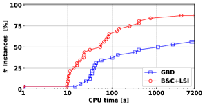
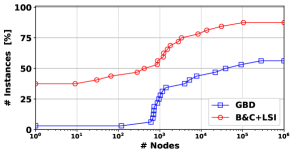
We now compare the performance of the proposed B&C algorithm equipped with the lifted submodular inequalities with the state-of-the-art GBD approach in Lin & Tian (2021), denoted by GBD. For GBD, we also employ a two-stage implementation, as our preliminary experiments showed that it is more efficient than the single-stage implementation in Lin & Tian (2021). The separation of Benders inequalities (6) is performed in a similar manner as in Section 5.2. Detailed computational results on instances in testsets T1 and T2 under settings GBD and B&C+LSI are shown in Tables 2 and 3, respectively. Similarly, to compare the effectiveness of the proposed lifted submodular inequalities and the Benders inequalities of Lin & Tian (2021), we report under column GI(%) the percentage gap improvement, defined by , where and are the upper bounds at the end of the first stage under settings B&C+LSI and GBD, respectively. In Figures 1 and 2, we further plot the performance profiles of the CPU time and number of explored nodes under settings GBD and B&C+LSI on instances in testsets T1 and T2, respectively.
We first compare the performanace of settings GBD and B&C+LSI on instances in testset T1. From Table 2, we observe that while the separation of the lifted submodular inequalities takes more computational efforts compared to that of the Benders inequalities, the use of the lifted submodular inequalities leads to a tighter formulation, resulting in a better upper bound. Indeed, with the lifted submodular inequalities, B&C+LSI consistently achieves a gap improvement GI(%) of over for instances in testset T1. With a tighter formulation, the rounding heuristic in B&C+LSI exhibits better performance, which can be confirmed from Table 2 that the lower bounds under B&C+LSI are much better than those under GBD. Due to the above advantages, B&C+LSI significantly outperforms GBD. Overall, B&C+LSI can solve out of all instances in testset T2, whereas GBD is only able to solve of them; for instances that can be solved by both settings, the average CPU time and average number of explored nodes under setting B&C+LSI are at least one magnitude smaller than those of GBD. The computational efficiency of B&C+LSI is more intuitively depicted in Figures 1(a) and 1(b), where we observe that approximately of the instances are solved by B&C+LSI within seconds, whereas only half of the instances are solved by GBD within the same period of time; more than half of the instances can be solved by B&C+LSI within nodes, whereas approximately instances can be solved by GBD within the same number of nodes.
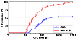
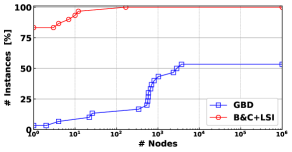
We now compare the performance of settings GBD and B&C+LSI on the large-scale CFLPLCR instances with partially binary rule in testset T2. As discussed at the end of Section 5.2, for the case that for all , the separation of (lifted) submodular inequalities in (24) admits an efficient exact algorithm. This is evident from Table 3 where the computational efforts required for the separation of the (lifted) submodular inequalities are relatively small. Moreover, as demonstrated in Corollary 4.5, for the case where for all , the (lifted) submodular inequalities are able to describe the convex hull of , and thus they enable to achieve a significantly better LP relaxation; see column GI(%) of Table 3. Therefore, B&C+LSI achieves a tremendously better performance than GBD. In particular, as shown in Table 3, B&C+LSI can solve all instances to optimality, whereas GBD fails to solve the instances with the number of facilities being or ; as depicted in Figures 2(a) and 2(b), the red circle lines corresponding to B&C+LSI are much “higher” than the blue square lines corresponding to GBD.
7 Conclusions
In this paper, we have investigated the polyhedral structure of the CFLPLCR and proposed an efficient B&C approach for solving large-scale problems. Our approach first establishes the submodularity of the probability function characterizing a customer’s probability to patronize new open facilities, and then uses the well-known submodular inequalities to describe the mixed 0-1 set defined by the hypograph of the probability function and the integrality constraints. Moreover, we strengthen the submodular inequalities by sequential lifting, obtaining an MILP formulation for the CFLPLCR described by the lifted submodular inequalities. Two key features of the proposed lifted submodular inequalities, which make them particularly well-suited to be embedded into a B&C algorithm, are as follows. First, their derivation explicitly takes the integrality constraints of the variables into consideration and they are guaranteed to define (strong) facet-defining inequalities of the convex hull of the considered mixed 0-1 set. Second, their computation admits an efficient pseudo-polynomial time algorithm. Numerical results showed that compared with the Benders inequalities in the state-of-the-art GBD algorithm whose derivation does not take the integrality constraints into consideration, the proposed lifted submodular inequalities are much more effective in terms of providing a tight LP relaxation bound. With this advantage, it is shown that the proposed B&C algorithm outperforms the state-of-the-art approach by at least one order of magnitude.
References
- Aboolian et al. (2007) Aboolian, R., Berman, O., & Krass, D. (2007). Competitive facility location and design problem. Eur. J. Oper. Res., 182, 40–62.
- Ahmed & Atamtürk (2011) Ahmed, S., & Atamtürk, A. (2011). Maximizing a class of submodular utility functions. Math. Program., 128, 149–169.
- Altekin et al. (2021) Altekin, F. T., Dasci, A., & Karatas, M. (2021). Linear and conic reformulations for the maximum capture location problem under multinomial logit choice. Optim. Lett., 15, 2611–2637.
- Aros-Vera et al. (2013) Aros-Vera, F., Marianov, V., & Mitchell, J. E. (2013). P-Hub approach for the optimal park-and-ride facility location problem. Eur. J. Oper. Res., 226, 277–285.
- Benati & Hansen (2002) Benati, S., & Hansen, P. (2002). The maximum capture problem with random utilities: Problem formulation and algorithms. Eur. J. Oper. Res., 143, 518–530.
- Beresnev (2013) Beresnev, V. (2013). Branch-and-bound algorithm for a competitive facility location problem. Comput. Oper. Res., 40, 2062–2070.
- Berman et al. (2009) Berman, O., Drezner, T., Drezner, Z., & Krass, D. (2009). Modeling competitive facility location problems: New approaches and results. In M. R. Oskoorouchi, P. Gray, & H. J. Greenberg (Eds.), Decision Technologies and Applications (pp. 156–181).
- Berman & Krass (1998) Berman, O., & Krass, D. (1998). Flow intercepting spatial interaction model: A new approach to optimal location of competitive facilities. Location Science, 6, 41–65.
- Biesinger et al. (2016) Biesinger, B., Hu, B., & Raidl, G. (2016). Models and algorithms for competitive facility location problems with different customer behavior. Ann. Math. Artif. Intell., 76, 93–119.
- Bodur et al. (2017) Bodur, M., Dash, S., Günlük, O., & Luedtke, J. (2017). Strengthened Benders cuts for stochastic integer programs with continuous recourse. INFORMS J. Comput., 29, 77–91.
- Bodur & Luedtke (2017) Bodur, M., & Luedtke, J. R. (2017). Mixed-integer rounding enhanced Benders decomposition for multiclass service-system staffing and scheduling with arrival rate uncertainty. Manag. Sci., 63, 2073–2091.
- Drezner et al. (2018) Drezner, T., Drezner, Z., & Zerom, D. (2018). Competitive facility location with random attractiveness. Oper. Res. Lett., 46, 312–317.
- Drezner & Eiselt (2024) Drezner, Z., & Eiselt, H. (2024). Competitive location models: A review. Eur. J. Oper. Res., 316, 5–18.
- Eiselt & Laporte (1997) Eiselt, H., & Laporte, G. (1997). Sequential location problems. Eur. J. Oper. Res., 96, 217–231.
- Fernández et al. (2017) Fernández, P., Pelegrín, B., Lančinskas, A., & Žilinskas, J. (2017). New heuristic algorithms for discrete competitive location problems with binary and partially binary customer behavior. Comput. Oper. Res., 79, 12–18.
- Fernández et al. (2021) Fernández, P., Pelegrín, B., Lančinskas, A., & Žilinskas, J. (2021). Exact and heuristic solutions of a discrete competitive location model with Pareto-Huff customer choice rule. J. Comput. Appl. Math., 385, 113200.
- Fischetti et al. (2016) Fischetti, M., Ljubić, I., & Sinnl, M. (2016). Benders decomposition without separability: A computational study for capacitated facility location problems. Eur. J. Oper. Res., 253, 557–569.
- Freire et al. (2016) Freire, A. S., Moreno, E., & Yushimito, W. F. (2016). A branch-and-bound algorithm for the maximum capture problem with random utilities. Eur. J. Oper. Res., 252, 204–212.
- Garey & Johnson (1978) Garey, M. R., & Johnson, D. S. (1978). “Strong” NP-completeness results: Motivation, examples, and implications. J. ACM, 25, 499–508.
- Gentile et al. (2018) Gentile, J., Alves Pessoa, A., Poss, M., & Costa Roboredo, M. (2018). Integer programming formulations for three sequential discrete competitive location problems with foresight. Eur. J. Oper. Res., 265, 872–881.
- Geoffrion (1972) Geoffrion, A. M. (1972). Generalized Benders decomposition. J. Optim. Theory Appl., 10, 237–260.
- Haase (2009) Haase, K. (2009). Discrete Location Planning. Technical Report WP-09-07 Institute of Transport and Logistics Studies University of Syndney.
- Haase & Müller (2014) Haase, K., & Müller, S. (2014). A comparison of linear reformulations for multinomial logit choice probabilities in facility location models. Eur. J. Oper. Res., 232, 689–691.
- Huff (1964) Huff, D. L. (1964). Defining and estimating a trading area. Journal of Marketing, 28, 34–38.
- Kress & Pesch (2012) Kress, D., & Pesch, E. (2012). Sequential competitive location on networks. Eur. J. Oper. Res., 217, 483–499.
- Krohn et al. (2021) Krohn, R., Müller, S., & Haase, K. (2021). Preventive healthcare facility location planning with quality-conscious clients. OR Spectrum, 43, 59–87.
- Küçükaydın et al. (2011) Küçükaydın, H., Aras, N., & Altınel, İ. K. (2011). A discrete competitive facility location model with variable attractiveness. J. Oper. Res. Soc., 62, 1726–1741.
- Lančinskas et al. (2017) Lančinskas, A., Fernández, P., Pelegín, B., & Žilinskas, J. (2017). Improving solution of discrete competitive facility location problems. Optim. Lett., 11, 259–270.
- Lančinskas et al. (2020) Lančinskas, A., Žilinskas, J., Fernández, P., & Pelegrín, B. (2020). Solution of asymmetric discrete competitive facility location problems using ranking of candidate locations. Soft Comput., 24, 17705–17713.
- Lin et al. (2022) Lin, Y., Wang, Y., Lee, L. H., & Chew, E. P. (2022). Profit-maximizing parcel locker location problem under threshold Luce model. Transp. Res. Part E Logist. Transp. Rev., 157, 102541.
- Lin & Tian (2021) Lin, Y. H., & Tian, Q. (2021). Branch-and-cut approach based on generalized Benders decomposition for facility location with limited choice rule. Eur. J. Oper. Res., 293, 109–119.
- Lin et al. (2024) Lin, Y. H., Tian, Q., & Zhao, Y. (2024). Unified framework for choice-based facility location problem. INFORMS J. Comput., online.
- Ljubić & Moreno (2018) Ljubić, I., & Moreno, E. (2018). Outer approximation and submodular cuts for maximum capture facility location problems with random utilities. Eur. J. Oper. Res., 266, 46–56.
- Mai & Lodi (2020) Mai, T., & Lodi, A. (2020). A multicut outer-approximation approach for competitive facility location under random utilities. Eur. J. Oper. Res., 284, 874–881.
- McFadden (1974) McFadden, D. (1974). Conditional logit analysis of qualitative choice behavior. In P. Zarembka (Ed.), Frontiers in Econometrics (pp. 105–142).
- Méndez-Vogel et al. (2023) Méndez-Vogel, G., Marianov, V., Lüer-Villagra, A., & Eiselt, H. (2023). Store location with multipurpose shopping trips and a new random utility customers’ choice model. Eur. J. Oper. Res., 305, 708–721.
- Nemhauser & Wolsey (1981) Nemhauser, G., & Wolsey, L. (1981). Maximizing submodular set functions: Formulations and analysis of algorithms. In P. Hansen (Ed.), North-Holland Mathematics Studies (pp. 279–301). volume 59.
- Nemhauser et al. (1978) Nemhauser, G. L., Wolsey, L. A., & Fisher, M. L. (1978). An analysis of approximations for maximizing submodular set functions—I. Math. Program., 14, 265–294.
- Plastria (2001) Plastria, F. (2001). Static competitive facility location: An overview of optimisation approaches. Eur. J. Oper. Res., 129, 461–470.
- Rahmaniani et al. (2017) Rahmaniani, R., Crainic, T. G., Gendreau, M., & Rei, W. (2017). The Benders decomposition algorithm: A literature review. Eur. J. Oper. Res., 259, 801–817.
- Richard (2011) Richard, J.-P. P. (2011). Lifting techniques for mixed integer programming. In J. J. Cochran, L. A. Cox, P. Keskinocak, J. P. Kharoufeh, & J. C. Smith (Eds.), Wiley Encyclopedia of Operations Research and Management Science.
- Shi et al. (2022) Shi, X., Prokopyev, O. A., & Zeng, B. (2022). Sequence independent lifting for a set of submodular maximization problems. Math. Program., 196, 69–114.
- Suárez-Vega et al. (2004) Suárez-Vega, R., Santos-Peñate, D. R., & Dorta-González, P. (2004). Competitive multifacility location on networks: The (rX p)-medianoid problem. J. Reg. Sci., 44, 569–588.
- Wolsey (1976) Wolsey, L. A. (1976). Technical note–facets and strong valid inequalities for integer programs. Oper. Res., 24, 367–372.
- Zhang et al. (2012) Zhang, Y., Berman, O., & Verter, V. (2012). The impact of client choice on preventive healthcare facility network design. OR Spectrum, 34, 349–370.
- Zhao et al. (2020) Zhao, Y., Guo, Y., Guo, Q., Zhang, H., & Sun, H. (2020). Deployment of the electric vehicle charging station considering existing competitors. IEEE Trans. Smart Grid, 11, 4236–4248.
Appendix A Proof of Proposition 3.6
Proof.
It suffices to consider the case . In this case, it is easy to see
Thus,
This shows statement (i).
Similarly, it is simple to check
Hence,
where the last inequality follows from , , and . Thus, statement (ii) also holds true. ∎
Appendix B Proof of Theorem 3.8
To prove Theorem 3.8, we need the following lemma.
Lemma B.1.
Let be the right-hand sides of inequalities (24), i.e.,
| (51) |
For any , it follows
| (52) |
where
| (53) |
Proof.
Given any , it follows
Together with the definition of , we have and . Thus equation (52) holds true. ∎
Proof of Theorem 3.8.
It suffices to show that every extreme point of is integral. Suppose, otherwise, that is a fractional extreme point of , i.e., for some . We have the following two cases.
-
(i)
holds for some . Let and , where is a sufficiently small value. By the definition of in (51), we have . From and the definitions of and in (53), it follows . Thus, . From Lemma B.1, this implies for all , and therefore . The proof of is similar. Since and , cannot be an extreme point of , a contradiction.
-
(ii)
holds for some and holds for all . Then, from the definition of in (53), this implies
(54) Let and , where is a sufficiently small value and . As is sufficiently small, by (54), we have , and thus
(55) (56) From , , , (55), and (56), it follows and . Therefore, using Lemma B.1, this implies and for all , and thus . Since and , point cannot be an extreme point of , a contradiction. ∎
Appendix C Proof of Theorem 4.6
We prove that problem (43) is as hard as the partition problem, which is NP-complete (Garey & Johnson, 1978). First, we introduce the partition problem: given a finite set of elements and a size for the -th element with , does there exist a partition such that ? Without loss of generality, we assume .
Given any instance of a partition problem, we construct an instance of problem (43) by setting , , , and for . As , the cardinality constraint in problem (43) becomes redundant. Thus, problem (43) reduces to
| (57) |
Letting where , it is simple to check that where the only maximum point is arrived at . Using this fact, holds if and only if holds for some , which is further equivalent to the existence of the partition problem with , that is, the answer to the partition problem is yes. Since the above transformation can be done in polynomial time and the partition problem is NP-complete, we conclude that problem (57) is NP-hard.